De-Sitter and double asymmetric brane worlds

Abstract

Asymmetric brane worlds with $dS$ expansion and static double kink topology are obtained from a recently proposed method and their properties are analyzed. These domain walls interpolate between two spacetimes with different cosmological constants. In the dynamic case, the vacua correspond to $dS$ and $AdS$ geometry, unlike the static case where they correspond to $AdS$ background. We show that is possible to confine gravity on such branes. In particular, the double brane world host two different walls, so that the gravity is localized on one of them.

PACS numbers: 04.20.-q, 11.27.+d, 04.50.+h

I Introduction

The idea that our universe could be a hypersurface embedded in a higher dimensional spacetime is being considered with raising interest. During recent years, new models have been explored Horava:1995qa ; Horava:1996ma ; Lukas:1998yy ; Lukas:1998qs ; Lukas:1999yn ; Arkani-Hamed:1998rs ; Antoniadis:1998ig ; Arkani-Hamed:1998nn ; Arkani-Hamed:1999hk ; Cremades:2002dh ; Kokorelis:2002qi which require either extra dimensions with compactification scale close to the limit of modern measurement of gravity (around millimeters) or noncompact extra dimensions. In the latter case, the visible universe is confined into a four-dimensional worldsheet (a $3$-brane) embedded in a larger spacetime. In particular, the five dimensional Randall-Sundrum model Randall:1999ee ; Randall:1999vf has received much attention since its birth because of its rich structure, which consists in a thin domain wall in a relatively simple conceptual framework.

Considering our four-dimensional universe as an infinitely thin domain wall is an idealization, and it is for this reason, that in more realistic models the thickness of the brane has been taken into account DeWolfe:1999cp ; Gremm:1999pj ; Csaki:2000fc ; Kehagias:2000au ; Kehagias:2000dg ; Behrndt:2001km ; Kobayashi:2001jd ; Campos:2001pr . The thick domain walls are solutions to Einstein’s gravity theory interacting with a scalar field, where the scalar field is a standard topological kink interpolating between the minima of a potential with spontaneously broken symmetry. We find that the coupled Einstein-scalar field system has singular solutions Guerrero:2005xx . This kind of solutions to the field equations is obtained from the usual regular thick domain walls, thus each regular solution is associated with an irregular one, just as it happens in classical sine-Gordon and KdV solitonic theory to accomplish complete integrability of these systems. In the present paper, we make simultaneous use of the regular and irregular solutions in order to generate novel brane worlds.

Due to the non-linearity and instability of the gravitational interactions, the inclusion of the gravitational evolution into a dynamic thick wall is a highly non-trivial problem. For this reason, there are not so many analytic solutions of a dynamic thick domain wall. In fact, to our knowledge, there exist in the literature only two solutions Goetz:1990 ; Sasakura:2002tq , with background metric on the brane given by a de-Sitter ($dS$) expansion, which resembles the Friedmann-Robertson-Walker metric, typical in a cosmological framework. In this work, we obtain another analytic solution of a thick brane with a $dS$ expansion, being $dS$ in one side and $AdS$ in other one along the perpendicular direction to the wall.

In the context of static domain wall spacetime, there are topological defects richer than the standard topological kinks. These configurations may be seen as defects that host internal structure, representing two parallel walls or double domain walls, whose properties have been studied in several papers: in Campos:1998db , using models described by a complex scalar field; in Morris:1995zp ; Bazeia:1995ui ; Edelstein:1997ej , in models described by two real scalar fields on flat spacetime; and in Gregory:2001xu , in brane scenarios involving two higher dimensions on curved spacetime. On the other hand, the models supported on a single real scalar field, with a $2$-kink profile have only been considered in Melfo:2002wd ; Bazeia:2003aw . In the present work, we shall deal with very specific models, described by a single real scalar field which couples with gravity on a conformal geometry with one extra dimension, where the wall interpolates between different $AdS$ vacua.

The purpose of this paper is to address the issue of localizing gravity in some new types of domain walls. In the next section, we review a method to obtain novel brane worlds from known ones developed in Guerrero:2005xx , and show that both branes are not physically equivalent. In sections III and IV, new domain wall solutions are found and analyzed with both a $dS$ expansion, and double kink topology. Finally, we summarize our results on section V.

II Approach to generate new solutions

The nonlinearity of the Einstein’s gravity theory interacting with a scalar field represents a strong difficulty when finding exact solutions to the system. In this sense, several formulations and methodologies Skenderis:1999mm ; DeWolfe:1999cp ; Guerrero:2002ki have been reported, where it is possible to reconsider the problem in a simpler way. Maintaining this focus, in this section, we will apply a new formulation based on the linearization of one of the equations of the system Guerrero:2005xx .

Consider the coupled Einstein-scalar field system

$$R_{\mu\nu}-\frac{1}{2}g_{\mu\nu}R=T_{\mu\nu},\qquad T_{\mu\nu}=\nabla_{\mu}\phi\nabla_{\nu}\phi-g_{\mu\nu}\left[\frac{1}{2}\nabla_{\sigma}\phi\nabla^{\sigma}\phi+V(\phi)\right],\qquad\nabla_{\mu}\phi\nabla^{\mu}\phi-\frac{dV(\phi)}{d\phi}=0,$$ (1)

where $\mu,\nu=0,...,4$.

We wish to find solutions to this coupled system with a planar parallel symmetry, where the scalar field $\phi$ is a function only of the perpendicular coordinate to the wall $x$. The most general metric of this kind is

$$ds^{2}=f^{2}(x)\left[-dt^{2}+e^{2\beta t}dy^{i}dy^{i}\right]+f^{2}(x)dx^{2},$$ (2)

where $i=1,2,3$. If ${\beta>0}$, we will have dynamic solutions; while if ${\beta=0}$, we will have static solutions. Following the recently proposed method in Guerrero:2005xx , let us $g$ be the inverse function of the metric factor $f$. Then the system (1) has associated an orthogonal set of solutions $\{g_{1},g_{2}\}$, for the same scalar field $\phi$, where

$$g_{2}(x)=g_{1}(x)\chi(x),\qquad\chi(x)\equiv\int_{x_{0}}^{x}\frac{1}{g_{1}^{2}(\xi)}\>d{\xi}$$ (3)

and the general solution

$$g(x)=g_{1}(x)\left[c_{1}+c_{2}\chi(x)\right],\qquad c_{1},c_{2}\in\Re$$ (4)

depends on two arbitrary constants.

We are interested in the realization of brane worlds on the geometry defined by $g$. In order to do this, we must guarantee that the spacetime does not present singularities along the extra coordinate that prevents the normalization of the zero mode of the spectra of gravitons, which is physically unacceptable. The possible singularities in (2) correspond to the zeros that (4) can take in some values of $x$. Considering $g_{1}$ as a continuos function without zeros, there are two cases where this can happen

1.-

If $c_{1}=0$ and $c_{2}\neq 0$, then $g$ will have a zero in $x_{0}$.

2.-

If $c_{1},c_{2}\neq 0$, then $g$ will have a zero in $x_{p}\in x$ when $\chi(x)|_{x_{p}}=-c_{1}/c_{2}.$

Therefore, to avoid divergences in (2), it is only necessary to choose appropriately the constants $c_{1}$ and $c_{2}$, so that its negative quotient does not belong to the range of $\chi(x)$, as can be deduced from the second condition.

As a final comment, equation (4) gives a mechanism to obtain new solutions to the coupled system from well known ones, compatible with the same scalar field but with different potentials. At this point, it is important to remark that spacetimes obtained from $g_{1}$ and $g$ with metric tensors $g_{1\mu\nu}$ and $g_{\mu\nu}$ are physically different, because it does not exist a diffeomorphism among them. In fact, these spacetimes are connected by a conformal transformation given by

$$g_{1\mu\nu}=\Omega^{2}g_{\mu\nu},\qquad\Omega\equiv c_{1}+c_{2}\chi(x).$$ (5)

In concordance with Wald:1984rg , the conformal transformations should not be understood as diffeomorphisms, but as applications that allow to connect two different spacetimes with identical causal structure. In this sense, we can conclude that the manifolds with metric tensors $g_{1\mu\nu}$ and $g_{\mu\nu}$ are physically non-equivalent.

III A new brane world with a de Sitter expansion.

Consider the embedding of a thick $dS$ $3$-brane into a five-dimensional bulk described by the metric (2), with a reciprocal metric factor given by

$$g_{1}(x)=\cosh^{\delta}(\beta x/\delta),\qquad 1/2>\delta>0,\qquad\beta>0.$$ (6)

In Ref.Goetz:1990 ; Gass:1999gk , it has been shown that this spacetime is a solution to the coupled equations (1) with

$$\phi=\phi_{0}\arctan\left(\sinh\ \beta x/\delta\right),\qquad\phi_{0}=\sqrt{3\delta(1-\delta)},$$ (7)

and

$$V_{1}(\phi)=\frac{1+3\delta}{2\delta}3\beta^{2}\left(\cos\phi/\phi_{0}\right)^{2(1-\delta)}.$$ (8)

The scalar field takes values $\pm\ \phi_{0}\pi/2$ at $x\rightarrow\pm\ \infty$, corresponding to two consecutive minima of the potential with cosmological constant $\Lambda=0$, and interpolates smoothly between these values; with $\delta$ playing the role of the wall’s thickness. It has been shown that this domain wall geometry localizes gravity on the wall in Wang:2002pk and has a well-defined distributional thin wall limit in Guerrero:2002ki .

Remarkably enough, not so many analytic solutions of a thick domain wall with $dS$ expansion are known. In fact, an exact solution on manifold with warped geometry is reported in Sasakura:2002tq ; and another one is given by (6, 7, 8). Moreover, this last one is the only dynamic domain wall on a spacetime with conformal gauge geometry encountered in the literature so far Goetz:1990 .

We wish to find another thick domain wall with $dS$ expansion in five-dimensions. From equation (4), choosing $c_{1}=1$, $c_{2}=\alpha$, with $g_{1}$ given by (6), we obtain

$$g=\cosh^{\delta}(\beta x/\delta)+\frac{i\ \alpha\delta}{\beta-2\beta\delta}\ \cosh^{(1-\delta)}(\beta x/\delta)\ \sinh^{-1}(\beta x/\delta)\ |\sinh\beta x/\delta|\ {}_{2}F_{1}[l,k,n,\cosh^{2}(\beta x/\delta)],$$ (9)

where ${}_{2}F_{1}$ is the hypergeometric function with $l=1/2-\delta,\ k=l+\delta$, and $n=l+1$. This solution represents a three-parameter family. Then, for simplicity we will consider the case $\delta=1/4$ without the loss of generality

$$g=\frac{1}{2\beta}\cosh^{1/4}(4\beta x)\ {\cal H}(x),\qquad 2\beta/\varepsilon>\alpha>0,\qquad\beta>0,$$ (10)

where ${\cal H}(x)\equiv 2\beta-\alpha\ iF[2i\beta x,2]$, $\ F$ is the incomplete first order elliptic function and $1/\alpha\neq{\rm Image}\{\chi(x)\}=\{-\varepsilon/2\beta,+\varepsilon/2\beta\}$ in order to prevent singularities in the metric tensor. Specifically for the case $\delta=1/4$, $\varepsilon=1.31103\$.

This spacetime is a solution to (1) with

$$\phi=\phi_{0}\arctan\left(\sinh\ 4\beta x\right),\qquad\phi_{0}=3/4,$$ (11)

and

$$V(\phi) = \frac{21}{8}\ |\cos\ 4\phi/3|^{3/2}\ {\cal H}(\phi)^{2}-\ 6\ \alpha\ |\cos\ 4\phi/3|^{2}\ {\cal H}(\phi)\ \tan(4\phi/3)-6\ \alpha^{2}\ |\cos\ 4\phi/3|^{1/2}.$$ (12)

Unlike the domain walls encountered in Goetz:1990 ; Sasakura:2002tq , for $x\rightarrow+\infty$ this spacetime is asymptotically $AdS$ with cosmological constant $-12\alpha\beta(1+\alpha\varepsilon/2\beta)\$ and for $\ x\rightarrow-\infty\$ is asymptotically $dS$ with cosmological constant $+12\alpha\beta(1-\alpha\varepsilon/2\beta)$. The asymmetry of this solution depends on the $\alpha$ parameter. In fact, for $\alpha\rightarrow 0$ a domain wall is obtained with reflection symmetry (6, 7, 8). For clarity, in Fig.1 we depict the metric factor $f=1/g$, the potential $V(\phi)$, and the density energy $\rho$ for $\alpha\rightarrow 0$ and $\alpha=3,5$.

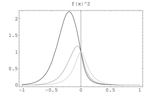
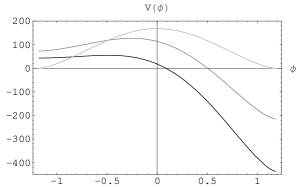
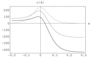
Figure 1: Plots of the metric factor (left), scalar potential (center), and the energy density (right) for $\beta=4$ and $\alpha\rightarrow 0$ and $\alpha=3,5$. Here and in the other figures the thickness of the lines increases with increasing $\alpha$.

Next, we shall show that this wall can confine gravity. In concordance with the straightforward generalization of the approach used to obtain the general fluctuations around a background metric presented in Castillo-Felisola:2004eg , the equations which describe linearized gravity in the transverse and traceless sector are

$$-\frac{1}{2}\nabla^{\sigma}\nabla_{\sigma}h_{\mu\nu}+R^{\sigma}{}_{(\mu\nu)}{}^{\varrho}h_{\sigma\varrho}+R^{\sigma}{}_{(\mu}h_{\nu)\sigma}=\frac{2}{3}h_{\mu\nu}V(\phi),$$ (13)

with $h_{\mu\nu}$ the metric perturbations. We write the metric fluctuations conveniently as

$$h_{ab}=e^{ip\cdot y}\ f(x)^{1/2}\ \psi_{ab}(x),$$ (14)

where $a,b=0,...,3$. From eq. (13) we have

$$(-\partial_{x}^{2}+V_{QM})\ \psi_{ab}=m^{2}\ \psi_{ab},$$ (15)

with $\ -m^{2}=p_{a}p^{a}-2\beta^{2}\$ the mass in the $dS$ background, and

$$V_{QM}(x)=\frac{15\beta^{2}}{\cosh^{2}(4\beta x){\cal H}(x)^{2}}\left[\alpha^{2}\cosh(4\beta x)+\frac{\alpha}{2}\cosh^{-1/2}(4\beta x)\sinh(8\beta x){\cal H}(x)-\frac{1}{40}(19-3\cosh 8\beta x){\cal H}(x)^{2}\right],$$ (16)

From eq. (15) we find that the spectrum of perturbations consists of a zero mode ($a,b$ indices omitted)

$$\psi_{0}=N\left[\frac{1}{2\beta}\cosh^{1/4}(4\beta x)\ {\cal H}(x)\right]^{-3/2},$$ (17)

and a set of continuous modes. On the other hand, from (16) we can see that $V_{QM}\rightarrow 9\beta^{2}/4$, as $\ |x|\rightarrow\infty$. Thus the continuous modes are separated by a mass gap $\ m^{2}>9\beta^{2}/4$, as in Wang:2002pk . In Fig. 2 we plot the potential $V_{QM}$, the corresponding zero mode, and the wave functions for massive modes. We see that the zero mode is bound on the brane, while mass modes move along the bulk, as expected. Moreover, the quantum mechanics potential is such that, in the transition region $dS-AdS$, there is a potential barrier in which the low energy massive modes experience a tunnel effect.

Figure 2: Plots of the $V_{QM}$ (dashed line), the zero mode (left) and the massive modes (right) for $\beta=4$, $\alpha=5$ and $m=7$.

IV Embedding of a new static thick brane world in an AdS background

Let us now consider a symmetric thick domain wall spacetime where the tensor metric is (2) for $\beta=0$, with

$$g_{1}(x)=\left[1+(\lambda\>x)^{2s}\right]^{1/2s},$$ (18)

where $\lambda\$ and $\ s\$ are real constants with $\ s\$ an odd integer. This solution was presented and broadly discussed in Melfo:2002wd and represents a two-parameter family of plane symmetric static double domain wall spacetime, being asymptotically $AdS_{5}$ with a cosmological constant $-6\ \lambda^{2}$.

The metric with reciprocal metric factor (18) is a solution to the coupled Einstein-scalar field equations (1) with

$$\phi=\phi_{0}\arctan(\lambda^{s}\>x^{s}),\qquad\phi_{0}=\frac{\sqrt{3(2s-1)}}{s},$$ (19)

and

$$V_{1}(\phi)=\frac{3}{2}\ \lambda^{2}\left[\tan(\phi/\phi_{0})\right]^{2(1-1/s)}\left[\cos(\phi/\phi_{0})\right]^{2(2-1/s)}\left[-1+2s-4\tan^{2}(\phi/\phi_{0})\right],$$ (20)

where $\phi$ interpolates between the two degenerate minima of $V(\phi)$, $\ \phi(\pm\infty)=\pm\ \phi_{0}\pi/2$. Similar solutions are also considered in Bazeia:2003aw .

In concordance with our approach, consider (4) with $g_{1}$ given by (18)

$$g=\left[1+(\lambda\>x)^{2s}\right]^{1/2s}\left(1+\alpha\>x\ {}_{2}F_{1}[l,k,n,-(\lambda\>x)^{2s}]\right),\qquad|\lambda|\ \frac{\Gamma(k)}{\Gamma(l)\ \Gamma(n)}>\alpha>0,$$ (21)

where $\ l=1/(2s),\ k=2l\$ and $\ n=1+l$. This spacetime is also solution to the coupled system with the scalar field (19) and

$$V(\phi) = -6\alpha^{2}\cos^{2/s}(\phi/\phi_{0})-\frac{3}{4}\sin^{2}(\phi/\phi_{0})\tan^{-2/s}(\phi/\phi_{0}){\cal K}(\phi)$$ (22)

$$\left\{16\alpha\tan^{1/s}(\phi/\phi_{0})+\cos^{-2/s}(\phi/\phi_{0})\left[5-2s-(3+2s)\cos(2\phi/\phi_{0})\right]{\cal K}(\phi)\right\}$$

where ${\cal K}(\phi)\equiv\lambda+\alpha\tan^{1/s}(\phi/\phi_{0})\ {}_{2}F_{1}[l,k,n,-\tan^{2}(\phi/\phi_{0})]$. This is a three-parameter family of plane symmetric static double domain wall spacetime without reflection symmetry along the direction perpendicular to the wall. These walls interpolate between $AdS$ asymptotic vacua with different cosmological constant $\ \Lambda_{-}=-6[\ |\lambda|\ \Gamma(k)-\alpha\Gamma(l)\Gamma(n)\ ]^{2}/\Gamma(k)^{2}\$ for $\ x<0\$ and $\ \Lambda_{+}=-6[\ |\lambda|\ \Gamma(k)+\alpha\Gamma(l)\Gamma(n)\ ]^{2}/\Gamma(k)^{2}\$ for $\ x>0$. For $\ \alpha\rightarrow 0\$ it reduces to (18, 19, 20); and if, additionally, $\ s=1\$ the regularized version of the Randall-Sundrum thin brane is obtained Gremm:1999pj ; Guerrero:2002ki . In Fig.3 we plot the metric factor, the potential $\ V(\phi)\$, and the energy density $\ \rho(x)\$ for different values of $\ \alpha$.

As consequence of the asymmetry of the spacetime (21), we see a difference in the amplitude of the peaks of $\rho(x)$, which indicates that the topological double kink host two branes whose energy densities differ considerably. Moreover, the lack of symmetry is notably observed in the asymptotically behavior of $\rho(x)$, which reveals the main characteristic of our solution: A double domain wall spacetime interpolating between different $AdS_{5}$ vacua.

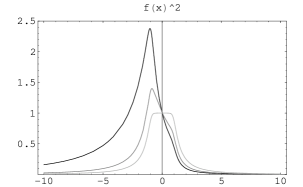
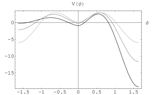
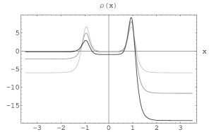
Figure 3: Plots of the metric factor (left), scalar potential (center), and the energy density (right) for $s=5,\ \lambda=1$ and $\alpha\rightarrow 0$ and $\alpha=0.2,0.4$.

Continuing with the analysis of the system, we would like to explore the thin wall limit of these configurations. Following Guerrero:2002ki , we introduce a new parameter $\delta$ by scaling the solution (21), so that the metric is now

$${}_{\delta}ds^{2}=g(x/\delta)^{-2\delta}\ (-dt^{2}+dy^{i}\ dy^{i})+g(x/\delta)^{-2}\ dx^{2}.$$ (23)

Observe that the scaling is performed so that this is still a solution to the Einstein-scalar field equations with

$$\phi(x)=\phi_{0}\arctan(\frac{\lambda^{s}x^{s}}{\delta^{s}}),\qquad\phi_{0}=\frac{\sqrt{3\delta(2s-1)}}{s},$$ (24)

and

$$V(\phi) = -6\alpha^{2}\cos^{2/s}(\phi/\phi_{0})-\frac{3}{4\delta}\sin^{2}(\phi/\phi_{0})\tan^{-2/s}(\phi/\phi_{0}){\cal K}(\phi)$$ (25)

$$\left\{16\alpha\delta\tan^{1/s}(\phi/\phi_{0})+\cos^{-2/s}(\phi/\phi_{0})\left[5-2s-(3+2s)\cos(2\phi/\phi_{0})+4(\delta-1)\sin^{2}(\phi/\phi_{0})\right]{\cal K}(\phi)\right\}.$$

The metric (23) is regular in the sense of Geroch:1987qn , thus all the curvature tensor fields make sense as distributions. Taking the distributional limit $\ \delta\rightarrow 0\$ of $G_{t}{}^{t}$ and $G_{x}{}^{x}$ we obtain

$$\lim_{\delta\rightarrow 0}G_{t}{}^{t}=-\Lambda_{+}\Theta(x)-\Lambda_{-}\Theta(-x)-3\lambda\frac{(2s-1)}{s}\frac{\Gamma(1-l)^{2}}{\Gamma(2-k)}\left(1+\frac{\alpha^{2}}{\lambda^{2}}\frac{\Gamma(l)^{2}\Gamma(n)^{2}}{\Gamma(k)^{2}}\right)\delta(x);$$ (26)

$$\lim_{\delta\rightarrow 0}G_{x}{}^{x}=-\Lambda_{+}\Theta(x)-\Lambda_{-}\Theta(-x),$$ (27)

where $\ \Theta\$ is the Heviside distribution. This clearly shows that the double configuration, in this limit, corresponds to an infinitely thin domain wall located at $\ x=0\$, tending asymptotically to $AdS_{5}$ spacetime with different cosmological constant at each side. For the case $\alpha\rightarrow 0$, it reduces to the thin wall limit associated to (18) reported in Melfo:2002wd . Remarkably enough, for $\delta\rightarrow 0$, (23) is not a regular metric in differentiable structure arising from the given chart, and we cannot use the approximation theorems of Geroch:1987qn in order to relate the limit of the curvature tensor distributions with the limit of the metric tensor field. Whether or not a metric is regular depends in general on differentiable structure imposed on the underlying manifold. A different chart may exist for which the resulting differentiable structure gives a regular metric, but this is not our concern here.

Let us return to solution (21) to carry out the analysis of gravitational fluctuations around this geometry. From eq.(13, 14) with

$$V_{QM}(x) = \frac{3\ \lambda\left[1+(\lambda\>x)^{2s}\right]^{-\frac{s+1}{s}}}{4x^{2}\ {\cal K}(x)^{2}}\left\{5\ \lambda(\alpha x)^{2}\left[1+(\lambda\>x)^{2s}\right]^{\frac{s-1}{s}}\right.$$ (28)

$$+(\lambda\>x)^{2s}\left[10\alpha\lambda x+\lambda\left[1+(\lambda\>x)^{2s}\right]^{-\frac{s-1}{s}}\left[2-4s+5(\lambda x)^{2s}\right]\right]$$

$$+\left.\alpha x(\lambda x)^{2s}\ \left[\lambda+{\cal K}(x)\right]{}_{2}F_{1}[l,k,n,-(\lambda x)^{2s}]\left[10\alpha\lambda x+\left[1+(\lambda\>x)^{2s}\right]^{-\frac{s-1}{s}}\left[2-4s+5(\lambda x)^{2s}\right]\right]\right\},$$

we solve for zero modes to get

$$\psi_{0}=N\ \lambda^{3/2}\left[1+(\lambda\>x)^{2s}\right]^{-3/(4s)}\ {\cal K}(x)^{-3/2}.$$ (29)

Remarkably, unlike the symmetric double-walls reported in Melfo:2002wd ; Bazeia:2003aw where zero mode is essentially constant between the two interfaces, the massless graviton on our asymmetric double-walls is strongly localized only on the interface centered around the lower minimum of the quantum-mechanic potential, which is in correspondence with the lower maximum of the energy density. For clarity, in Fig.4 we depict the zero mode and the potential $V_{QM}$ for the same values of the parameters. This asymmetric configuration is an exotic example of two parallel walls with different energy densities, where the gravity selects the brane associated to the lower energy conditions as a scenario in order to accomplish our universe.

Figure 4: Plots of the $V_{QM}$ (dashed line), the zero mode (left) and the massive modes (right) for $s=5,\ \lambda=1$, $\alpha=0.4$ and $m=0.9$.

In Fig. 4 we can also see that the wave functions for massive modes move with relative freedom along the extra dimension, where those with the lower energy experience an attenuation due to the presence of the potential barrier localized near the wall with greater energy density.

Finally, for scaled metric (23) we find that the linearized equation of motion for tensor fluctuations cannot be rewritten as a Schrödringer equation. Moreover, the metric is not regular for $\delta\rightarrow 0$ in the sense of Geroch:1987qn . Hence, four-dimensional gravity cannot be reproduced on the thin wall limit and a brane-world in this case is inviable.

V Conclusions

In this paper we find two brane worlds embedded in a spacetime with a non-conventional geometry. Both solutions were obtained applying the method developed in Guerrero:2005xx , which is supported in the linearization of one of the equations of the coupling Einstein scalar field.

In the first case, we studied thick domain walls with $dS$ expansion in a novel geometry that tends asymptotically to different cosmological constants, being $dS$ in one side and $AdS$ in the other one, along the perpendicular direction to the wall. This asymmetry is a consequence of the behavior of the scalar field, which interpolates between two non-degenerate minima of a scalar potential without $Z_{2}$ symmetry. These walls are a generalization of the first dynamic solution to coupling (1) reported in Goetz:1990 ; Gass:1999gk . We showed that the zero mode of the graviton spectrum is localized on the asymmetric brane and there exists a gap between this state and the massive modes, which is a generic property of the $dS$ branes.

Finally, in the second case, we considered asymmetric static double-brane world with two different walls; arising from a scalar potential without $Z_{2}$ symmetry. These branes are embedded in a $AdS_{5}$ spacetime and in the thin wall limit, the energy density and pressure of these walls correspond to a single infinitely sheet with different cosmological constants on each side of the wall. The thick configuration turned out to be a generalization of the regularized (thick) Randall-Sundrum scenario studied in Melfo:2002wd . We found that the zero mode of the metric fluctuation is localized on one of the walls, the one corresponding to the conditions of minimum energy; and that the massive modes are not bounded on any of the walls.

References

- (1) P. Horava and E. Witten, Nucl. Phys. B 460, 506 (1996) [arXiv:hep-th/9510209].
- (2) P. Horava and E. Witten, Nucl. Phys. B 475, 94 (1996) [arXiv:hep-th/9603142].
- (3) A. Lukas, B. A. Ovrut, K. S. Stelle and D. Waldram, Phys. Rev. D 59, 086001 (1999) [arXiv:hep-th/9803235].
- (4) A. Lukas, B. A. Ovrut and D. Waldram, Phys. Rev. D 60, 086001 (1999) [arXiv:hep-th/9806022].
- (5) A. Lukas, B. A. Ovrut and D. Waldram, Phys. Rev. D 61, 023506 (2000) [arXiv:hep-th/9902071].
- (6) N. Arkani-Hamed, S. Dimopoulos and G. R. Dvali, Phys. Lett. B 429, 263 (1998) [arXiv:hep-ph/9803315].
- (7) I. Antoniadis, N. Arkani-Hamed, S. Dimopoulos and G. R. Dvali, Phys. Lett. B 436, 257 (1998) [arXiv:hep-ph/9804398].
- (8) N. Arkani-Hamed, S. Dimopoulos and G. R. Dvali, Phys. Rev. D 59, 086004 (1999) [arXiv:hep-ph/9807344].
- (9) N. Arkani-Hamed, S. Dimopoulos, G. R. Dvali and N. Kaloper, Phys. Rev. Lett. 84, 586 (2000) [arXiv:hep-th/9907209].
- (10) D. Cremades, L. E. Ibanez and F. Marchesano, Nucl. Phys. B 643, 93 (2002) [arXiv:hep-th/0205074].
- (11) C. Kokorelis, Nucl. Phys. B 677, 115 (2004) [arXiv:hep-th/0207234].
- (12) L. Randall and R. Sundrum, Phys. Rev. Lett. 83, 3370 (1999) [arXiv:hep-ph/9905221].
- (13) L. Randall and R. Sundrum, Phys. Rev. Lett. 83, 4690 (1999) [arXiv:hep-th/9906064].
- (14) O. DeWolfe, D. Z. Freedman, S. S. Gubser and A. Karch, Phys. Rev. D 62, 046008 (2000) [arXiv:hep-th/9909134].
- (15) M. Gremm, Phys. Lett. B 478, 434 (2000) [arXiv:hep-th/9912060].
- (16) C. Csaki, J. Erlich, T. J. Hollowood and Y. Shirman, Nucl. Phys. B 581, 309 (2000) [arXiv:hep-th/0001033].
- (17) A. Kehagias and K. Tamvakis, Phys. Lett. B 504, 38 (2001) [arXiv:hep-th/0010112].
- (18) A. Kehagias and K. Tamvakis, Mod. Phys. Lett. A 17, 1767 (2002) [arXiv:hep-th/0011006].
- (19) K. Behrndt and G. Dall’Agata, Nucl. Phys. B 627, 357 (2002) [arXiv:hep-th/0112136].
- (20) S. Kobayashi, K. Koyama and J. Soda, Phys. Rev. D 65, 064014 (2002) [arXiv:hep-th/0107025].
- (21) A. Campos, Phys. Rev. Lett. 88, 141602 (2002) [arXiv:hep-th/0111207].
- (22) R. Guerrero, R. Ortiz, R. O. Rodriguez and R. Torrealba, arXiv:gr-qc/0504080.
- (23) G. Goetz, J. Math. Phys. 31 2683 (1990).
- (24) N. Sasakura, JHEP 0202, 026 (2002) [arXiv:hep-th/0201130].
- (25) A. Campos, K. Holland and U. J. Wiese, Phys. Rev. Lett. 81, 2420 (1998) [arXiv:hep-th/9805086].
- (26) J. R. Morris, Phys. Rev. D 51, 697 (1995).
- (27) D. Bazeia, R. F. Ribeiro and M. M. Santos, Phys. Rev. D 54, 1852 (1996).
- (28) J. D. Edelstein, M. L. Trobo, F. A. Brito and D. Bazeia, Phys. Rev. D 57, 7561 (1998) [arXiv:hep-th/9707016].
- (29) R. Gregory and A. Padilla, Phys. Rev. D 65, 084013 (2002) [arXiv:hep-th/0104262].
- (30) A. Melfo, N. Pantoja and A. Skirzewski, Phys. Rev. D 67, 105003 (2003) [arXiv:gr-qc/0211081].
- (31) D. Bazeia, C. Furtado and A. R. Gomes, JCAP 0402, 002 (2004) [arXiv:hep-th/0308034].
- (32) K. Skenderis and P. K. Townsend, Phys. Lett. B 468, 46 (1999) [arXiv:hep-th/9909070].
- (33) R. Guerrero, A. Melfo and N. Pantoja, Phys. Rev. D 65, 125010 (2002) [arXiv:gr-qc/0202011].
- (34) R. M. Wald, “General Relativity”
- (35) R. Gass and M. Mukherjee, Phys. Rev. D 60, 065011 (1999) [arXiv:gr-qc/9903012].
- (36) A. z. Wang, Phys. Rev. D 66, 024024 (2002) [arXiv:hep-th/0201051].
- (37) O. Castillo-Felisola, A. Melfo, N. Pantoja and A. Ramirez, Phys. Rev. D 70, 104029 (2004) [arXiv:hep-th/0404083].
- (38) R. Geroch and J. H. Traschen, Phys. Rev. D 36, 1017 (1987).