String Gas Cosmology

Abstract

We present a critical review and summary of String Gas Cosmology. We include a pedagogical derivation of the effective action starting from string theory, emphasizing the necessary approximations that must be invoked. Working in the effective theory, we demonstrate that at late-times it is not possible to stabilize the extra dimensions by a gas of massive string winding modes. We then consider additional string gases that contain so-called enhanced symmetry states. These string gases are very heavy initially, but drive the moduli to locations that minimize the energy and pressure of the gas. We consider both classical and quantum gas dynamics, where in the former the validity of the theory is questionable and some fine-tuning is required, but in the latter we find a consistent and promising stabilization mechanism that is valid at late-times. In addition, we find that string gases provide a framework to explore dark matter, presenting alternatives to $\Lambda$CDM as recently considered by Gubser and Peebles. We also discuss quantum trapping with string gases as a method for including dynamics on the string landscape.

I Introduction

String theory continues to have a number of challenges to address if it is to be made experimentally verifiable. Cosmology offers an exciting opportunity to explore such challenges, since the early universe provides conditions where string dynamics would play a vital role. To investigate the predictions of string cosmology it is important to have concrete constructions of string models in backgrounds that are compatible with our understanding of the early universe. In particular, this presents us with the challenge of finding solutions of string theory in time-dependent backgrounds and at nonzero temperature.

The usual method for constructing models of string cosmology is to compactify any extra dimensions and then focus on the low energy, massless degrees of freedom. However, this presents a problem since the low energy equations of motion lack potentials to fix the massless moduli. For cosmology, this implies the existence of many light scalars, which if not fixed at late-times would seem to contradict current observations. Nevertheless, a few light scalars could prove valuable to cosmology, since they could address the issue of dark energy, dark matter, or provide a theoretical motivation for inflation.

String or Brane Gas Cosmology (SGC) is an approach to string cosmology which began with the pioneering work of Brandenberger and Vafa in Brandenberger and Vafa (1989). They presented an elegant explanation for the dimensionality of space-time by considering the effects of massive string modes on the evolution of the early universe. Since this seminal paper, considerable effort has gone into realizing whether such a scenario is possible. In fact, the cosmology of string gases has lead to interesting conclusions beyond those originally proposed by Brandenberger and Vafa. In this paper we attempt to present a pedagogical, yet critical, review of the string gas approach.

In Section II, we review the origin of the effective action of string cosmology as it arises from string theory in the low energy - weak coupling limit. For homogeneous fields, this effective theory exhibits a dynamical symmetry, so-called scale factor duality. We present the BPS fundamental string solution and corresponding stress-energy tensor for the special case of a time-independent background. In Section III, after explicitly stating the assumptions of the SGC approach, we generalize the fundamental strings to a time-dependent background treating them as an ideal gas. We derive the corresponding energy and pressure and discuss the duality properties of the spectrum. In Section IV, we return to the Brandenberger and Vafa mechanism and review recent work that challenges the heuristic argument. However, we point out that this argument is not quintessential to string gas cosmology. Next, we consider the effect of a classical string gas on the time-dependent background. This has been examined in the literature from both the $10D$ String frame and $4D$ Einstein frame perspectives. We review these works, stressing the importance that physical quantities are frame independent. Using this, we demonstrate that string gases of purely winding modes are not enough to stabilize the extra dimensions.

A possible resolution to these problems consists of considering string states that become massless at critical values of the radion (scale of the extra dimension). These gases can drive the evolution of the radion to the location which minimizes the pressure of the gas. However, we will see that this approach suffers from fine-tuning issues: first, each string gas configuration can lead to a different attractor point on the moduli space; second, if the radion starts far from the attractor point, the density of the gas will exceed the energy cutoff of the effective theory, questioning the validity of the approach.

In Section V, we present a resolution to these fine-tuning problems, by considering the quantum aspects of the string gas. This approach, known as quantum moduli trapping Kofman et al. (2004); Watson (2004a), takes the initial theory to contain only the low energy massless modes of the string. Then, as the radion nears a point of enhanced symmetry (ESP) where additional states become light, the states must be included in the effective action. This leads to particle production of the additional light states. Once on-shell, these states result in a confining potential, since their energy density grows as the radion departs from the ESP.

In Section VI, we consider the possibility of obtaining observational signatures from string gases. We demonstrate that remnant strings in the extra dimensions provide natural candidates for the alternative $\Lambda$CDM model proposed recently by Gubser and Peebles in Gubser and Peebles (2004b). We also comment on the possibility of combining string gases with a period of cosmological inflation.

In Section VII we conclude. In the appendices we provide a short review on conformal transformations and dimensional reduction, necessary for going between the $10D$ String frame and $4D$ Einstein frames.

In this review, we attempt to provide a comprehensive survey of the existing SGC literature, focusing on the string theory origin and the importance of moduli stabilization. For complementary reviews with emphasis on cosmological aspects, we refer the reader to Brandenberger (2005a, b).

II Dynamics of Strings in Time-Dependent Backgrounds

A closed string in a background generated by its bosonic, massless modes is described by a nonlinear sigma model Callan et al. (1985)

$$S_{\sigma}=-\frac{1}{4\pi\alpha^{\prime}}\int d^{2}\sigma\Bigl{(}\sqrt{-\gamma}\gamma^{ab}G_{\mu\nu}(X)\;\partial_{a}X^{\mu}\partial_{b}X^{\nu}+\epsilon^{ab}B_{\mu\nu}(X)\;\partial_{a}X^{\mu}\partial_{b}X^{\nu}\Bigr{)},$$ (1)

where $\gamma^{ab}$ is the world-sheet metric, $(2\pi\alpha^{\prime})$ is the inverse string tension, $G_{\mu\nu}$ is the background space-time metric, $B_{\mu\nu}$ is the background antisymmetric tensor. Our convention in this review will be that coordinates of the full space-time are denoted by $X^{\mu}$ with $\mu=0\ldots D-1$, where $D$ is the space-time dimension. Spatial dimensions parameterized by $X^{i}$ are denoted by indices $i,j=1\ldots D-1$, compact dimensions are given by coordinates $Y^{m}$ with $m,n$ running over compact spatial coordinates, and $\sigma^{a}$ with $\sigma^{0}\equiv\tau,\sigma^{1}\equiv\sigma$ are the worldsheet coordinates.

In addition to the action above, one can add a topological term

$$S_{\phi}=-\frac{1}{4\pi}\int d^{2}\sigma\sqrt{\gamma}\phi(X)R^{(2)},$$ (2)

where $\phi$ is the background dilaton, which is coupled to the world-sheet Ricci scalar $R^{(2)}$. The string coupling is then given in terms of the vacuum expectation value of the dilaton $g_{s}=e^{\phi_{0}}$.

Varying the action (1) with respect to the fields, $X^{\mu}$, gives the string equations of motion in a general space-time

$$\partial_{a}\Bigl{(}\sqrt{\gamma}\gamma^{ab}\partial_{b}X^{\mu}\Bigr{)}+\Gamma^{\mu}_{\;\lambda\nu}\sqrt{\gamma}\gamma^{ab}\partial_{a}X^{\lambda}\partial_{b}X^{\nu}+\frac{1}{2}H^{\mu}_{\;\lambda\nu}\epsilon^{ab}\partial_{a}X^{\lambda}\partial_{b}X^{\nu}=0.$$ (3)

In addition, one must satisfy the constraint equations

$$G_{\mu\nu}(X)\Bigl{(}\partial_{a}X^{\mu}(\sigma,\tau)\partial_{b}X^{\nu}(\sigma,\tau)-\frac{1}{2}\gamma_{ab}\gamma^{cd}\partial_{c}X^{\mu}\partial_{d}X^{\nu}\Bigr{)}=0.$$ (4)

The background fields, $G_{\mu\nu},B_{\mu\nu}$, and $\phi$, are realized as couplings of the non-linear sigma model as can be seen from the action above. This model possesses a conformal symmetry classically, but this is spoiled at the quantum level by anomalies; the couplings evolve in accordance with the corresponding beta functions. This is equivalent to demanding that the trace of the world-sheet stress tensor given by

$$T^{a}_{a}=\beta^{G}_{\mu\nu}\sqrt{\gamma}\gamma^{ab}\partial_{a}X^{\mu}\partial_{b}X^{\nu}+\beta^{B}_{\mu\nu}\epsilon^{ab}\partial_{a}X^{\mu}\partial_{b}X^{\nu}+\beta^{\phi}\sqrt{\gamma}R^{(2)},$$ (5)

vanishes, where the $\beta$ functions are found, (e.g. by the background field method) to be Callan et al. (1985)

$$\beta^{G}_{\mu\nu}=\Bigl{(}R_{\mu\nu}+2\nabla_{\mu}\nabla_{\nu}\phi-\frac{1}{4}H_{\mu\kappa\sigma}H_{\nu}^{\;\kappa\sigma}\Bigr{)}+{\cal O}(\alpha^{\prime}),$$

$$\beta^{B}_{\mu\nu}=\Bigl{(}\nabla^{\kappa}H_{\kappa\mu\nu}-2\nabla^{\kappa}\phi H_{\kappa\mu\nu}\Bigr{)}+{\cal O}(\alpha^{\prime}),$$

$$\beta^{\phi}=\frac{1}{\alpha^{\prime}}\Bigl{(}\frac{D-26}{48\pi^{2}}\Bigr{)}+\Bigl{(}4\nabla_{\kappa}\phi\nabla^{\kappa}\phi-4\nabla_{\kappa}\nabla^{\kappa}\phi-R+\frac{1}{12}H_{\kappa\mu\nu}H^{\kappa\mu\nu}\Bigr{)}+{\cal O}(\alpha^{\prime}),$$ (6)

with $H=dB$ denoting the field strength associated with the field $B_{\mu\nu}$. Keeping terms tree level in $\alpha^{\prime}$, these equations of motion can be derived from those of the low energy effective action of supergravity in $D$ space-time dimensions

$$S_{0}=\frac{1}{2\kappa_{D}^{2}}\int d^{D}x\sqrt{-G}e^{-2\phi}\Bigl{(}R+c+4(\nabla\phi)^{2}-\frac{1}{12}H^{2}\Bigr{)}\,,$$ (7)

where $c$ vanishes in the critical case, $D=26$ $(D=10)$ for the bosonic (super) string, and acts as a cosmological constant in the noncritical case. In the case $D\leq 10$, the prefactor takes the form $2\kappa_{D}^{2}=(2\pi\sqrt{\alpha^{\prime}})^{D-2}g_{s}^{2}(2\pi)^{-1}=16\pi G_{D}$ with $l_{s}=\sqrt{\alpha^{\prime}}$ the string length and $G_{D}$ the $D$ dimensional Newton constant. By noting this prefactor we see that this action is not only tree level in $\alpha^{\prime}$, but it is also tree level in $g_{s}=e^{\phi_{0}}$ where $\phi_{0}$ is the expectation value of the dilaton .

The above action exhibits a new symmetry, scale factor duality, that is not found in pure general relativity. To see this, let us consider cosmological solutions, ignoring flux for the moment and working in the critical dimension ($c=0$).We take the metric and dilaton to have the form

$$ds^{2}=-dt^{2}+\sum_{i=1}^{d}a_{i}^{2}(t)\,dx_{i}^{2},$$

$$a_{i}\equiv e^{\lambda_{i}(t)},\;\;\;\;\phi=\phi(t),\;\;\;\;d=D-1,$$ (8)

where the spatial directions are taken to be toroidal. It will prove useful to perform a field redefinition and introduce the shifted dilaton,

$$\varphi=2\phi-\ln V=2\phi-\sum_{i=1}^{d}\lambda_{i}.$$ (9)

Plugging this ansatz for the fields into the action (7) one finds that the action is invariant under the transformation

$$a_{i}\rightarrow\frac{1}{a_{i}},\;\;\;\;\;\;\lambda_{i}\rightarrow-\lambda_{i},\;\;\;\;\;\;\varphi\rightarrow\varphi.$$ (10)

This symmetry is known as scale factor duality, and has interesting consequences for cosmology. In particular, it tells us that the effective field theory of dilaton gravity for a small scale factor is equivalent to that for a large scale factor.

In addition to the low-energy action for the massless modes above, one may consider the addition of classical or quantum string matter. One approach that was first advocated in Dabholkar et al. (1996, 1990); Dabholkar and Harvey (1989) is to include the action (1) as a phenomenological matter source for the background fields in (7). There are many interpretations of what such a term may represent. In the supergravity (SUGRA) solutions presented in Dabholkar et al. (1996, 1990); Dabholkar and Harvey (1989), the authors observed that the string source was required at the origin to complete the solution. It has also been argued that this action can be added as a method for taking into consideration quantum corrections coming from higher genus worldsheets (see e.g. Tseytlin (1992); de Alwis and Sato (1996)). This interpretation is clear from the additional power of $g_{s}^{2}$ that appears in front of the action (1) relative to (7).

If we consider a single string source for the background fields the total action becomes,

$$S=S_{0}+S_{\sigma}.$$ (11)

Varying this action we recover the equation of motion of the string (3), the constraints (4), and the background equations sourced by the string which take the form

$$R_{\mu\nu}+2\nabla_{\mu}\nabla_{\nu}\phi-\frac{1}{4}H_{\mu\kappa\sigma}H_{\nu}^{\;\kappa\sigma}=-\frac{\kappa^{2}_{D}e^{2\phi}}{2\pi\alpha^{\prime}\sqrt{-G}}\int d^{2}\sigma\sqrt{\gamma}\gamma^{ab}\partial_{a}X^{\mu}\partial_{b}X^{\nu}\delta^{(D)}(x-X(\sigma)),$$

(12)

$$\nabla_{\mu}\left(e^{-2\phi}H^{\mu\nu\rho}\right)=\frac{\kappa_{D}^{2}}{\pi\alpha^{\prime}\sqrt{-G}}\int d^{2}\sigma\epsilon^{ab}\partial_{a}X^{\nu}\partial_{b}X^{\rho}\delta^{(D)}(x-X(\sigma)),$$ (13)

$$4\nabla_{\kappa}\phi\nabla^{\kappa}\phi-4\nabla_{\kappa}\nabla^{\kappa}\phi-R+\frac{1}{12}H_{\kappa\mu\nu}H^{\kappa\mu\nu}=0.$$ (14)

From (12) we see that the stress-energy tensor of a single string is

$$T_{\mu\nu}\equiv\frac{2}{\sqrt{-G}}\frac{\delta S_{\sigma}}{\delta G_{\mu\nu}}=-\frac{1}{2\pi\alpha^{\prime}\sqrt{-G}}\int d^{2}\sigma\sqrt{\gamma}\gamma^{ab}\partial_{a}X^{\mu}\partial_{b}X^{\nu}\delta^{(D)}(x-X(\sigma)).$$ (15)

These equations, along with (3) and (4), represent a system of a single string in the presence of its background massless modes. Solving these equations would seem extremely difficult given the non-linearity of the problem. However, static solutions were found some time ago Dabholkar et al. (1996, 1990); Dabholkar and Harvey (1989) and these so-called F-string solutions were shown to preserve some supersymmetries and exhibit BPS-like properties similar to solitons. In particular, two parallel strings satisfy a no-force condition, since the gravitational attraction is canceled by the scalar exchange of the dilaton and flux. Instead, in SGC we will be interested in solutions generated by a gas of strings at finite temperature and in cosmological (time-dependent) background fields.

III Cosmology with String Gases

We now want to attempt to solve for the background fields allowing for conditions indicative of early universe cosmology. As mentioned in the previous section, generically the equations resulting from (3) are very difficult to solve. However, by invoking some approximations that are not in conflict with cosmological observation, the equations can be made tractable. We will now explicitly state these approximations leaving a discussion of their limitations to follow.

III.1 Assumptions of the string gas approach

• Homogeneous Fields:   We will assume that the background fields (i.e. metric, flux, and dilaton) are homogeneous and therefore at most functions of time. The generalization to inhomogeneous fields was addressed in Watson and Brandenberger (2004); Watson (2004b); Battefeld et al. (2005).

• Adiabatic approximation:   We will assume that the background fields are evolving slowly enough that higher derivative corrections, i.e. $(\alpha^{\prime})$ corrections, can be ignored. This means that locally, string sources won’t be influenced by the expansion and their evolution can be characterized by their scaling behavior.

• Weak Coupling:   We will work in the region of weak coupling (i.e. $g_{s}\ll 1$), and we will choose initial conditions for the dilaton that preserve this condition. Thus, higher orders corrections in $g_{s}$, can be neglected.

• Toroidal Spatial Dimensions:   We assume that all spatial dimensions are toroidal and therefore admit non-trivial one cycles. In the past this assumption was believed to be crucial, however it was later shown that this condition may be relaxed in some cases, allowing for more phenomenologically motivated backgrounds Easther et al. (2002).

From the point of view of cosmology, all of these approximations are familiar. However, both the adiabatic and weak coupling approximation are very restrictive from the string theory perspective. The string corrections that we are choosing to ignore may be very important for early universe cosmology, especially near cosmological singularities. The motivation here is to take a modest approach by slowly turning on stringy effects, as one extrapolates the known cosmological equations backward in time to better understand the departures from standard big-bang cosmology. This is to be contrasted to models of string cosmology that invoke supersymmetry to avoid higher order corrections. From the cosmological standpoint, one could argue that these models are less realistic since supersymmetry should not be expected to hold in conditions favorable to the early universe, i.e. time-dependent, finite temperature backgrounds. It is certainly premature to claim one has a well established understanding of string theory in cosmological backgrounds, but one hopes by the SGC approach to better understand what role strings play in the early universe.

III.2 Energy and pressure of a string gas

Given the assumptions stated above, we now want to find cosmological solutions to the equations (12)-(14), given the presence of a string gas. The time-dependent background fields are

$$ds^{2}=-dt^{2}+\sum_{i=1}^{d}a_{i}^{2}(t)\,dx_{i}^{2},$$

$$a_{i}\equiv e^{\lambda_{i}(t)},\;\;\;\;\phi=\phi(t),\;\;\;\;B_{\mu\nu}=0,\;\;\;\;d=D-1.$$ (16)

The adiabatic approximation implies that the local effects of expansion on the string can be neglected, allowing us to simplify the string equation of motion (3) to

$$\partial_{a}\Bigl{(}\sqrt{\gamma}\gamma^{ab}\partial_{b}X^{\mu}\Bigr{)}+\Gamma^{\mu}_{\;\lambda\nu}\sqrt{\gamma}\gamma^{ab}\partial_{a}X^{\lambda}\partial_{b}X^{\nu}\approx\left(\partial_{\tau}^{2}-\partial_{\sigma}^{2}\right)X^{\mu}(\sigma,\tau)=0,$$ (17)

where we have fixed the gauge of the worldsheet metric to $\gamma_{ab}=f(\tau,\sigma)\eta_{ab}$, with $\eta_{ab}=diag(-1,1)$. In this gauge the constraints (4) become

$$G_{\mu\nu}\left(\dot{X}^{\mu}\dot{X}^{\nu}+\acute{X}^{\mu}\acute{X}^{\nu}\right)=0$$ (18)

$$G_{\mu\nu}\dot{X}^{\mu}\acute{X}^{\nu}=0,$$ (19)

where $\dot{X}\equiv\partial_{\tau}X$ and $\acute{X}\equiv\partial_{\sigma}X$. Since the $X^{\mu}$ satisfy a free wave equation, their solution can be decomposed into left and right movers

$$X^{\mu}=X^{\mu}_{L}(\tau+\sigma)+X^{\mu}_{R}(\tau-\sigma),$$

$$X^{\mu}_{R}=x_{R}^{\mu}+\sqrt{\frac{\alpha^{\prime}}{2}}p_{R}^{\mu}(\tau-\sigma)+i\sqrt{\frac{\alpha^{\prime}}{2}}\sum_{n\neq 0}\frac{1}{n}\alpha_{n}^{\mu}e^{-in(\tau-\sigma)},$$

$$X^{\mu}_{L}=x_{L}^{\mu}+\sqrt{\frac{\alpha^{\prime}}{2}}p_{L}^{\mu}(\tau+\sigma)+i\sqrt{\frac{\alpha^{\prime}}{2}}\sum_{n\neq 0}\frac{1}{n}\tilde{\alpha}^{\mu}_{n}e^{-in(\sigma+\tau)},$$ (20)

where $x_{R}$ and $x_{L}$ are the center of mass position, $p_{R}^{\mu}$ and $p_{L}^{\mu}$ are the center of mass momentum, and $\alpha$ ($\tilde{\alpha}$) after quantization are the operators associated with right (left) moving oscillations of the string. If we take some of the spatial dimensions to be compact with coordinates $Y^{m}$, then the center of mass momenta become

$$p_{R}^{m}=\frac{\sqrt{\alpha^{\prime}}}{R}\;n^{m}-\frac{R}{\sqrt{\alpha^{\prime}}}\;\omega^{m},$$

$$p_{L}^{m}=\frac{\sqrt{\alpha^{\prime}}}{R}\;n^{m}+\frac{R}{\sqrt{\alpha^{\prime}}}\;\omega^{m},$$ (21)

where $R$ is the scale factor in the $m$th compact direction, $n_{m}$ is an integer giving the charge of the Kaluza-Klein momentum in that direction and $\omega^{l}=G^{mn}\omega_{m}$ is an integer giving the winding number of the wound string (Note: The placing of the indices is important, for a generic metric $G_{mn}$, $n^{m}$ and $\omega_{m}$ are not integers.). It is important to note that we are again invoking the adiabatic approximation, since we are treating the scale factor $R$ as a constant (locally).

If we now substitute this solution into the constraint equation (18) and use the gauge choice $X^{0}=E\tau\sqrt{\alpha^{\prime}}$ we find

$$-G_{00}\dot{X}^{0}\dot{X}^{0}\equiv\alpha^{\prime}E^{2} = G_{ij}\left(\dot{X}^{i}\dot{X}^{j}+\acute{X}^{i}\acute{X}^{j}\right)+G_{mn}\left(\dot{Y}^{m}\dot{Y}^{n}+\acute{Y}^{m}\acute{Y}^{n}\right)$$ (22)

$$= \alpha^{\prime}\vec{P}^{\;2}+\frac{(p_{L}^{2}+p_{R}^{2})}{2}+2\left(N_{L}+N_{R}+a_{L}+a_{R}\right),$$

which is the mass shell condition for the string $E^{2}=\vec{P}^{\;2}+M^{2}$. The constants $a_{R}$ and $a_{L}$ have been added to account for normal ordering, with $a_{R}=a_{L}=-1$ for the bosonic string. For the heterotic string $a_{L}=-1$ and $a_{R}=-\frac{1}{2}$ for the Neveu-Schwarz sector, while $a_{R}=0$ for the Ramond-Ramond sector, and $N_{R}$ ($N_{L}$) is the excitation number of the right (left) oscillators. We have also allowed for the presence of non-compact dimensions $X^{i}$, for which the string has center of mass momentum $\vec{P}$ and we have used $X^{i}=\sqrt{\alpha^{\prime}}\vec{P}\tau$. Using the other constraint (19) we find the level matching condition

$$p_{L}^{2}-p_{R}^{2}=4n_{m}\omega^{m}=4(N_{R}-N_{L}+a_{R}-a_{L}).$$ (23)

From the string mass spectrum we immediately see that strings are invariant under the same duality as the massless background fields. Namely, the string spectrum is unchanged under the transformation

$$\frac{R}{\sqrt{\alpha^{\prime}}}\rightarrow\frac{\sqrt{\alpha^{\prime}}}{R}\;\;\;\;n\longleftrightarrow\omega,$$ (24)

which suggests that strings at small scale factor $\frac{1}{R}$, behave the same as strings at large scale factor $R$. This property of the spectrum, known as t-duality, is a very important property of strings and suggests that their effects on cosmological backgrounds may differ greatly from that of ordinary point particles Brandenberger and Vafa (1989).

We would now like to reconsider the stress energy tensor (15) for this string configuration (see e.g. de Vega and Sanchez (1995)). The $T^{00}$ component is given by

$$T^{00} = -\frac{1}{2\pi\alpha^{\prime}\sqrt{-G}}\int d^{2}\sigma\sqrt{\gamma}\gamma^{ab}\partial_{a}X^{0}\partial_{b}X^{0}\delta^{(D)}(x^{\mu}-X(\sigma)^{\mu})$$ (25)

$$= \frac{1}{2\pi\alpha^{\prime}\sqrt{-G}}\int d^{2}\sigma\left(\dot{X}^{0}\dot{X}^{0}-\acute{X}^{0}\acute{X}^{0}\right)\delta^{(D)}(x^{\mu}-X^{\mu}(\sigma)),$$

where we have again used the conformal gauge for the worldsheet metric $g_{ab}=f(\tau,\sigma)\eta_{ab}$. Noting our previous choice of $X^{0}=\sqrt{\alpha^{\prime}}E\tau$, we find

$$T^{00} = \frac{1}{2\pi\alpha^{\prime}|\dot{X}^{0}|\sqrt{-G}}\int^{2\pi\sqrt{\alpha^{\prime}}}_{0}d\sigma\;\delta^{(D-1)}(x^{i}-X^{i}(\sigma))\left(\dot{X}^{0}\dot{X}^{0}-\acute{X}^{0}\acute{X}^{0}\right)_{\tau=\tau(X^{0})}$$ (26)

$$= \frac{E}{\sqrt{-G_{{D-1}}}}\;\delta^{(D-1)}(x^{i}-X^{i}(\sigma)),$$

which is the energy density of a single string with the delta function enforcing that there is no contribution unless we are at the position of the string. The explicit formula for the energy of the string in terms of its oscillations and momentum then follows from (III.2) and the constraint (22)

$$E=\sqrt{\vec{P}^{\;2}+G^{mn}\left(n_{m}+\frac{\omega_{m}}{\alpha^{\prime}}\right)\left(n_{n}+\frac{\omega_{n}}{\alpha^{\prime}}\right)+\frac{4}{\alpha^{\prime}}\left(N_{L}+a_{L}\right)},$$ (27)

where we have eliminated $N_{R}$ in favor of the other quantum numbers by using (23). It is straight forward to generalize this to a gas of $N$ strings. We simply average over the delta function sources and the energy density of the string gas is

$$\rho=\sum_{s}\tilde{n}_{s}E_{s},$$ (28)

where the sum is over all species $s$ and $\tilde{n}_{s}={N_{s}}{V}^{-1}$ is the number density of the string gas in spatial volume $V$, with a particular set of quantum numbers $n,\omega,N_{L},N_{R}$. We will assume that the gas is a perfect fluid and non-interacting. Therefore, we can find the pressure in the $i$-th direction

$$p_{i}=-\frac{1}{V}\frac{\partial(\rho V)}{\lambda_{i}},$$ (29)

where $a_{i}=\exp(\lambda_{i})$ is the scale factor in the $i$-th direction.

As a simple example, let us consider two bosonic string gases ($a_{L}=a_{R}$) composed of strings wrapping the compact dimensions ($\omega_{m}\neq 0,n_{m}=N_{L}=N_{R}=0$) and strings with momentum in the compact dimensions ($n_{m}\neq 0,\omega_{m}=N_{L}=N_{R}=0$). Assuming we can neglect the non-compact momenta, $\vec{P}=0$, their energy density and pressure are given by

$$\rho_{w} = \sum_{l=1}^{d}\tilde{n}_{w}^{(l)}e^{\lambda_{l}(t)},\;\;\;\;\;\;\rho_{m}=\sum_{l=1}^{d}\tilde{n}_{m}^{(l)}e^{-\lambda_{l}(t)},$$

$$p_{w}^{(l)} = -\tilde{n}_{w}e^{\lambda_{l}(t)},\;\;\;\;\;\;\;\;\;\;p^{(l)}_{m}=\tilde{n}_{m}e^{-\lambda_{l}(t)},$$ (30)

where we now take $d$ to denote the number of compact directions and we have vanishing pressure in the $D-1-d$ non-compact dimensions. We have lifted the scale factors $R_{i}=e^{\lambda_{i}}$ to time-dependent functions using the adiabatic approximation, with $V(t)$ the time-dependent spatial volume ($\ln V(t)=\sum_{i=1}^{D-1}\lambda_{i}(t)$). For simplicity we have absorbed the winding and momentum numbers $\omega,n$ into the number density of winding and momentum modes in the $l$th direction $\tilde{n}_{w}^{(l)}$ and $\tilde{n}_{m}^{(l)}$. We have also renormalized the mass to remove the tachyonic zero point energy $a_{L}$, which would be automatically removed in the case of heterotic strings. Here we do this by hand, since we are mainly concerned with the scaling of the string energy with $\lambda_{i}$. Given an isotropic distribution of strings in the extra dimensions, we find that the equation of state for winding and momentum modes is

$$p_{w}=-\frac{1}{d}\rho_{w},\;\;\;\;\;\;\;\;\;\;p_{m}=\frac{1}{d}\rho_{m},$$ (31)

respectively. We see that winding modes contribute negative pressure whereas the momentum modes scale as radiation filling the extra dimensions. To close this section, we have found that under the assumption that the string gas can be modeled as a perfect fluid, the stress energy tensor of a single string (15) can be generalized to

$$T^{\mu}_{\nu}=diag\left(-\rho,p_{1},p_{2},\ldots,p_{D-1}\right),$$ (32)

where the energy density and pressure are given by (28) and (29), respectively.

IV Classical dynamics of string gases

IV.1 Initial Conditions and the Dimensionality of Space-time

One of the successes of SGC is the possibility to explain the emergence of three large and isotropic spatial dimensions, while six remain stabilized near the string scale. In this way, SGC is the only cosmological model thus far that has attempted to explain the dimensionality of space-time dynamically. The qualitative argument, due to Brandenberger and Vafa Brandenberger and Vafa (1989), was that winding string modes can maintain equilibrium in at most three spatial dimensions. This is based on the simple fact that $p$ dimensional objects can generically intersect in at most $2p+1$ dimensions and the intuition that string interactions are due to intersections. They argued that once the winding modes annihilate with anti-winding modes, three spatial dimensions would be free to expand while the remaining six should remain confined by winding modes near the string scale. Winding modes were shown to possess such confining behavior quantitatively in Tseytlin and Vafa (1992). There, the importance of the dilaton was stressed because this led to the observation that the negative pressure of winding modes leads to contraction rather than accelerated expansion. It was later observed that the dilaton is not the critical feature restoring the Newtonian intuition per se, rather it is the effect of anisotropies . In fact, it was shown many years ago that string winding modes could lead to confinement in the case of general relativity Kripfganz and Perlt (1988).

This counting argument was verified numerically in a static background, focusing on cosmic strings in Sakellariadou (1996) (see also Cleaver and Rosenthal (1995) ) and later extended to the case of branes in Alexander et al. (2000), where it was argued that the strings remain the important objects, since branes fall out of equilibrium sooner than strings, leading to a hierarchial structure of dimensions. The setup has been generalized to more complex topologies Easther et al. (2002); Easson (2003); Biswas (2004) and many authors elaborated on these basic arguments Kaya and Rador (2003); Rador (2005a, c, b); Kaya (2003, 2004); Arapoglu and Kaya (2004); Kaya (2005b, a); Kim (2004); Park et al. (2000); Hotta et al. (1997); Deo et al. (1992, 1991). The t-duality of branes was discussed in the context of SGC in Boehm and Brandenberger (2003). Other recent attempts to address dimensionality making use of branes in a different way have appeared in Durrer et al. (2005); Karch and Randall (2005).

Despite the appeal of the BV argument, there remain serious challenges for its quantitative realization. As a first step, a study in eleven dimensional supergravity Easther et al. (2003) employing a fixed wrapping matrix (based on the counting argument) yielded indeed the predicted anisotropic expansion. However, the internal dimensions were not stabilized, but simply grew slower. This work was extended in Easther et al. (2004) by studying the coupled Einstein-Boltzmann equations for a thermal brane gas. It was found that only highly fine tuned initial conditions yield the desired outcome. The most recent study Easther et al. (2005) focusing on dilaton gravity confirmed these results: either all dimensions grow large, since the string gas annihilated entirely, or all dimension stay small, since the string gas froze out – intermediate solutions can only be achieved by fine-tuning the initial conditions. It was also observed that a string gas freezes out quite quickly due to the coupling to the rolling dilaton Danos et al. (2004).

A crucial input is the interaction rate of strings Polchinski (1988) that lead to the corresponding Boltzmann equation. The interaction probability relies on the value of $g_{s}$ and therefore the dilaton. As the dilaton runs to weak coupling this means that interaction probabilities go to zero. Secondly, viewing interactions as intersections is an entirely classical argument. At the level of supergravity one has exchange of closed strings that mediate interactions. This increases the probability of interaction, since closed string exchange can take place in any number of dimensions with the only dilution being due to the force following a generalized Newton law, i.e. $F\sim\frac{1}{r^{D-2}}$. Henceforth, the conclusion of Easther et.al.’s investigations have been that compactification of all or none of the dimensions is the most probable configuration Easther et al. (2005, 2003, 2002). However, this analysis was done given our rather limited knowledge of string theory dynamics. In particular, our knowledge of cosmological solutions when all radii are taken to be at the string scale is sketchy at best. A more complete knowledge of both curvature corrections ($\alpha^{\prime}$) and the strong coupling behavior of the theory could certainly change this outcome. Moreover, time dependent solutions of the full string theory continue to be an avenue that is being actively pursued. It will be interesting to see if the BV argument will hold, given a more complete understanding of string theory dynamics. While awaiting this progress, we will simply assume in what follows that winding modes were able to annihilate in three spatial dimensions, causing those to be free to expand while a winding mode gas remains in the other six. Thus, our initial conditions will be no more unnatural than those of usual models of cosmology.

IV.2 Cosmological Evolution in the Presence of a String Gas

Anticipating the $D=3+1+6$ split, due to the annihilation of the winding modes in three dimensions, let us consider the following background field configuration

$$ds^{2}=-dt^{2}+e^{2\lambda(t)}d\vec{x}^{2}+e^{2\nu(t)}d\vec{y}^{2},$$ (33)

$$H_{3}=h\;dx^{1}\wedge dx^{2}\wedge dx^{3},\;\;\;\;\;\;\phi=\phi(t),$$ (34)

where $H_{3}$ is a constant three form flux restricted by the expected symmetries (namely, $3+1+6$). We want to consider these background fields in the equations of motion (12)-(14), with the string sources replaced by the averaged stress tensor of the string gas (32). We have

$$R_{\mu\nu}+2\nabla_{\mu}\nabla_{\nu}\phi-\frac{1}{4}H_{\mu\kappa\sigma}H_{\nu}^{\;\kappa\sigma}=16\pi G_{10}e^{2\phi}T_{\mu\nu},$$ (35)

$$\nabla_{\mu}\left(e^{-2\phi}H^{\mu\nu\rho}\right)=0,$$ (36)

$$4\nabla_{\kappa}\phi\nabla^{\kappa}\phi-2\nabla_{\kappa}\nabla^{\kappa}\phi-\frac{1}{6}H_{\kappa\mu\nu}H^{\kappa\mu\nu}=16\pi G_{10}e^{2\phi}T,$$ (37)

where $G_{10}$ is the ten-dimensional Newton constant, $T\equiv T^{\mu}_{\mu}$ is the trace of the stress tensor, and we have used the trace of (35) to rewrite the last equation. Writing (37) in this form allows us to make the important observation that (ignoring flux) the dilaton can only evolve if matter is not conformal (i.e. $T\neq 0$). This condition will be respected by string gases in general, and it is this important observation that makes string cosmology (dilaton gravity) very different from ordinary cosmology. The flux equation (36) is trivially satisfied given the ansatz for the background fields and we assume that the flux of the strings themselves average to zero. The remaining equations can be written in the form

$$c-3\dot{\lambda}^{2}-6\dot{\nu}^{2}+\dot{\varphi}^{2}-\frac{h^{2}}{2}e^{-6\lambda}=e^{\varphi}E,$$ (38)

$$\ddot{\lambda}-\dot{\varphi}\dot{\lambda}-\frac{1}{2}h^{2}e^{-6\lambda}=\frac{1}{2}e^{\varphi}P_{3}$$ (39)

$$\ddot{\nu}-\dot{\varphi}\dot{\nu}=\frac{1}{2}e^{\varphi},P_{6},$$ (40)

$$\ddot{\varphi}-3\dot{\lambda}^{2}-6\dot{\nu}^{2}=\frac{1}{2}e^{\varphi}E,$$ (41)

where we have introduced the energy $E=\rho V$, we define the scaled pressure $P_{i}=p_{i}V$, and $\varphi$ is the shifted dilaton (9). The first equation is an energy constraint, which if satisfied at some initial time will remain satisfied for all times. The sources obey a conservation equation,

$$\dot{E}+3\dot{\lambda}P_{3}+6\dot{\nu}P_{6}=0.$$ (42)

From the above equations we see that the term involving flux will be negligible at late-times, since it scales as $a^{-6}$. However, in the early universe as one approaches the cosmological singularity this term may become vital to understanding the dynamics Friess et al. (2004). Also, if we decide to work in the non-critical theory (i.e. $c\neq 0$), we see that $c$ acts as an effective cosmological constant.

IV.3 Summary of 10d Dynamics and Moduli Stabilization

We will now briefly review the results of various authors in studying the system of equations (38)-(41), where it will be assumed that $h=0$ and $c=0$ unless noted otherwise. In Brandenberger et al. (2002); Easson (2001), the above equations were studied with energy and pressure given by a gas of string winding modes as in (III.2). There it was shown that the universe remains in a period of cosmological loitering until all of the winding modes have annihilated. Once the winding modes have all annihilated the dimensions are freed to grow large. It was observed that the period of loitering would resolve the horizon problem, without the need to invoke cosmological inflation. These results agree with the earlier study in Tseytlin and Vafa (1992), where it was shown that the negative pressure of the string winding modes leads to contraction in string cosmology, not inflation. In Watson and Brandenberger (2003b), the effect of the winding mode annihilation processes on the three dimensions growing large was shown to lead to a natural explanation for the observed isotropy of our universe. This resulted from the annihilation rate depending on the size of the dimension and the expansion rate depending on the number of winding modes present. Moreover, the string winding modes annihilate into unwound closed string loops, or momentum modes, which we saw from (31) scale as radiation (d=3 in this case). Thus, it was shown that a large, three dimensional, radiation dominated universe naturally evolves from SGC.

In the above investigations, the stabilization of the other six dimensions was assumed a priori. In Watson and Brandenberger (2003a), these dimensions were included and filled with a gas of string winding modes and a gas of string momentum modes, with energy and pressure as in (III.2). It was shown that as the three spatial dimensions continue to grow large, the six compact dimensions will oscillate about the self-dual radius, since winding modes were unable to annihilate in these dimensions via the BV argument discussed above. The oscillations are the result of the negative pressure of the string winding modes ($p_{w}=-\tilde{n}e^{\nu}$) driving the radius to smaller values and the positive pressure of the string momentum modes ($p_{m}=\tilde{n}_{m}e^{-\nu}$) driving the radius to larger values. For an equal number of winding and momentum modes (i.e. $\tilde{n}_{w}=\tilde{n}_{m}$) one finds that the evolution is driven to the critical radius, the so-called self-dual radius $\nu=0$ or $b=\sqrt{\alpha^{\prime}}$ where the total pressure vanishes and t-duality is restored. In order for stabilization to occur it was crucial that the dilaton ran to weak coupling. This running of the dilaton leads to a damping effect of the internal dimensions, as can be seen in Figure 1. The running of the dilaton implies that the Newton constant will evolve and this will prove problematic at late-times. However, the important point here is that during the early stages of the evolution, the extra dimensions are naturally led to the self-dual radius. In fact, the important point stressed in Watson and Brandenberger (2003a) and later elaborated on in Patil and Brandenberger (2005); Watson (2004a); Patil and Brandenberger (2006) is the presence of additional massless string states that become massless at the self-dual radius and should therefore be considered in the low energy action. We will see in Section V that these states can have a very important effect resulting in a stabilization mechanism for the extra dimensions.

So far, we have ignored the problem of inhomogeneities, since we have assumed all the background fields to be homogeneous. This problem was considered at late-times in Watson and Brandenberger (2004) and Watson (2004c), where it was shown that the dilaton again plays a vital role. It was found that as long as the dilaton continues to roll towards weak coupling, perturbations will be under control and stability of the string frame radion will persist. So it would appear that the dilaton plays a very important role in SGC, but as we will see in the next section, it must ultimately be stabilized if SGC is to agree with observation.

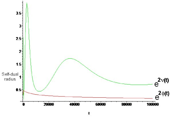
Figure 1: This graph shows the primary results of Watson and Brandenberger (2003a), where stabilization of the string frame radion (green or light line) in the presence of string winding and momentum modes was demonstrated. The damping of the oscillations relied crucially on the dilaton running slowly to weak coupling (red or dark line).

The role of inhomogeneities at early-times is a much more challenging problem. As we approach the cosmological singularity, we might hope that the finiteness of strings would resolve the singularity and/or provide a bounce. Although many different approaches have been attempted (see e.g. Khoury et al. (2002); Gasperini and Veneziano (2003)), no convincing models have been found Polchinski (2005). This seems a promising area for SGC to investigate, given the various duality properties exhibited by the string gas and background fields Brandenberger and Vafa (1989). The dynamics of SGC as the singularity is approached has been largely ignored due to the lack of control of string corrections and the expected breakdown of the assumptions stated in Section III. One attempt at understanding the evolution is the work of Friess et al. (2004), where it was found that the background flux would play a crucial role and could no longer be ignored. It will be interesting to see how string winding modes and strings as local sources of flux can effect the evolution towards the singularity. This presents an important challenge for SGC.

Before closing this section, we would like to briefly mention some other consideration of SGC dynamics that have appeared in the literature. The assumption of toroidal geometry used in (38)-(41) was generalized to orbifold backgrounds in Easther et al. (2002), where it was found that the confining behavior of winding modes still persists even in the absence of non-trivial homotopy. Interactions of the string winding and momentum mode gases were considered in both Bastero-Gil et al. (2002) and Danos et al. (2004), where in the former it was argued that correlations between the winding and momentum modes lead to modified dispersion relations that may help explain the small value of the cosmological constant. In addition to the study of the equations (38)-(38), attempts to extend SGC to M-theory via its connection with $11D$ SUGRA was considered in Alexander (2003); Easther et al. (2005, 2003); Campos (2005b). Campos has considered the importance of background flux in SGC Campos (2003, 2004, 2005a). Whereas in Brandenberger et al. (2005) the effects of strings as sources of flux was considered, and in particular their ability to stabilize shape moduli in addition to the radion. The idea of inflation or cosmic acceleration from SGC was discussed in Brandenberger et al. (2004); Kaya (2004); Parry and Steer (2002) and remains a difficult challenge for SGC. We refer the reader to our references for addition papers on SGC.

IV.4 $4D$ Dynamics and the Effective Potential

Thus far the stability analysis of the extra dimensions has been carried out in the string frame. In this frame it has been shown that the radion is stabilized at the self-dual radius by the competing negative and positive pressure of the stringy matter, along with damping provided by the dilaton which continues to run to weak coupling. However, at late-times an evolving dilaton is problematic for both particle phenomenology and moduli stabilization. In fact, any evolving gravitational scalar will lead to a changing gravitational constant $G_{N}$, which is tightly constrained by fifth force experiments (see e.g. Gubser and Khoury (2004)). Moreover, because the Einstein frame radion is actually a linear combination of the string frame dilaton and radion, we will find that the extra dimensions will be unstable as long as the dilaton evolves. We will briefly discuss possibilities for dynamically stabilizing the dilaton in the next section, but let us first review the problem of stability as discussed in Battefeld and Watson (2004) (see also Berndsen and Cline (2004); Berndsen et al. (2005); Easson and Trodden (2005)).

In order to examine the late time behavior of SGC it is most appropriate to work in the $4D$ Einstein frame. Since we have focused on homogeneous fields, the physical quantities originating from these equations are equivalent to those of the $10D$ string frame we have considered thus far; this is simply the consistency of dimensional reduction. The $10D$ Einstein frame metric can be rewritten in terms of the string frame scale factors and dilaton as

$$ds^{2}_{E}=-dt_{E}^{2}+e^{\phi/2}a^{2}(t)d\vec{x}^{2}+e^{\phi/2}b^{2}(t)d\vec{y}^{2},\;\;\;\text{with}\;\;\;dt_{E}^{2}=e^{\phi/2}dt_{s}^{2}$$ (43)

which immediately allows one to see the problem. Even if one fixes $b(t)$, the dilaton evolution still prevents stabilization of the Einstein frame radion. We see that in this case the Einstein frame makes this instability manifest in a simple way. However, the same conclusion could have been reached in the string frame by more complicated methods, such as identifying the physical radion and examining the corresponding two-point function. The important point is that the two frames are physically equivalent, but the instability is manifest in the Einstein frame. In addition to the problem of the dilaton, we will see that from the $4D$ Einstein frame additional problems arise regarding the dilution of our string matter as a source of stabilization.

Beginning from the $10D$ string frame action (7) one can reduce to the $4D$ Einstein frame by a conformal transformation followed by field redefinitions to canonically normalize the scalars. We leave the details to the appendix, where we find

$$S_{4}=\int d^{4}x\sqrt{-{g}}\Biggl{(}\frac{1}{16\pi G}\Bigl{[}R[{g}_{\mu\nu}]-\frac{1}{2}{g}^{\mu\nu}{\nabla}_{\mu}\psi{\nabla}_{\nu}\psi-\frac{1}{2}{g}^{\mu\nu}{\nabla}_{\mu}{\phi}{\nabla}_{\nu}{\phi}\Bigr{]}-e^{4\phi-\sqrt{\frac{d}{2}}\psi}\mathcal{V}^{(4+d)}_{s}(\lambda,\varphi,\psi)\Biggr{)}.$$

where again we neglect flux and work in the critical dimensions $c=0$ and where the $4D$ Newton constant is given by $16\pi G={2\pi\alpha^{\prime}g_{s}^{2}}$. The canonically normalized scalars, $\phi$ and $\psi$ are then $4D$ fluctuations about the fixed values for the dilaton and radion, respectively. The $10D$ string frame potential $\mathcal{V}^{(4+d)}_{s}$ includes the effects of any wrapped branes or strings, flux, cosmological constant or any other contribution to the energy density.

As a simple example, consider a cosmological constant arising in the $10D$ string frame, such as appears in the RR sector of massive Type II-A supergravity. We see that in the $4D$ Einstein frame this term is no longer constant

$$\mathcal{V}^{(4+d)}_{s}\sim\Lambda\;\;\;\longrightarrow\;\;\;\mathcal{V}^{(4)}_{E}=\frac{e^{4\phi-\sqrt{\frac{d}{2}}\psi}}{(2\pi\sqrt{\alpha^{\prime}})^{4}}\,\Lambda,$$ (44)

and if we assume weak coupling, i.e. $\phi\rightarrow-|\phi|$, we see that one gets a exponential runaway potential.

We would now like to see if the situation improves in SGC, where it seemed earlier that wrapped strings could stabilize the extra dimensions. We are interested in potentials coming from wrapped and moving branes and strings on the compact space. Assuming the string frame metric to have the form

$$ds^{2}=-dt^{2}+a^{2}(t)dx^{2}+b^{2}(t)dy^{2},$$ (45)

we can write the $10D$ string frame potential as

$$\mathcal{V}^{(4+d)}_{s}=\mu\frac{Nb^{k}}{a^{3}b^{d}}$$ (46)

where $\mu=(2\pi\sqrt{\alpha^{\prime}})^{-4}$ and following the notation in the appendix we have absorbed a factor of $(2\pi\sqrt{\alpha^{\prime}})^{6}$ coming from the compactification into the definition of $\mathcal{V}_{s}^{(4+d)}$. The number of strings (branes) is given by $N$ and $k\leq|d|$ is the type of strings (branes) (e.g., $k=2$ is a wound 2-brane and $k=-1$ is a string with Kaluza-Klein momentum in one compact direction). Of course, this expression is just a generalization of our earlier expression (III.2), for the energy density of winding and momentum string gases. The reduction to $4D$ leaves the potential unchanged, but we must transform the scale factor $a(t)$ when moving to the Einstein frame, i.e. $\tilde{a}(t)=e^{-\varphi}a(t)$, where $\varphi$ is the canonical $4D$ dilaton $\varphi=2\phi-d\ln b$ and $\tilde{a}(t)$ is the Einstein frame scale factor. The potential becomes

$$\mathcal{V}^{(4+d)}_{s}=\mu\tilde{n}e^{-\frac{3}{2}\varphi}b^{k-d}=\mu\tilde{n}e^{-3\phi}b^{k+\frac{d}{2}},$$ (47)

where $\tilde{n}$ is the number density in the Einstein frame and we have expressed the potential in terms of the unshifted dilaton. Comparing this potential with the action (IV.4) we find that the potential in the $4D$ Einstein frame is

$$\mathcal{V}^{(4)}_{E}=\mu\tilde{n}e^{\phi}b^{k-\frac{d}{2}}=\mu\tilde{n}e^{-|\phi|}\exp\left[\left({\frac{2k-d}{2\sqrt{2d}}}\right)\psi\right],$$ (48)

where in the last step we have expressed the radion in terms of the canonical variable $\psi$ and we have assumed the dilaton evolves to weak coupling. From this potential we can see that a confining potential only arises if $k\geq\frac{d}{2}$. For the case of a winding string ($k=1$) this is only true for a single extra dimension $d=1$ and even then there is an overall factor of the dilaton diluting this potential. We conclude that a gas of purely winding strings is not enough to stabilize the extra dimensions.

Given this negative outcome, we would now like to consider a gas composed of a less restrictive string configuration. Let us consider the stress energy tensor for a gas of heterotic strings given by (28), (29), and (32). The energy of the individual string is given by (27) and in the case of the heterotic string takes the form

$$E_{HE}=\sqrt{G^{mn}\left(n_{m}+\frac{\omega_{m}}{\alpha^{\prime}}\right)\left(n_{n}+\frac{\omega_{n}}{\alpha^{\prime}}\right)+\frac{4}{\alpha^{\prime}}\left(N_{L}-1\right)},$$ (49)

and the level matching condition follows from (23) as

$$n_{m}\omega^{m}=N_{R}-N_{L}+\frac{1}{2},$$ (50)

where we have used $a_{L}=-1$ and $a_{R}=\frac{1}{2}$ for the heterotic string and we have again assumed that $\vec{P}=0$. We are interested in ground state configurations of the string, which in the case of NS Heterotic strings means setting the right oscillators to their minimum value, $N_{R}=\frac{1}{2}$ (see Polchinski (1998b) for details). We then want to consider non-oscillatory states ($N_{L}=0$), since we are interested in the terms that contain explicit dependence on the scale factor of the extra dimensions. With these assumptions the energy and constraint become

$$E_{(N_{L}=0,N_{R}=\frac{1}{2},\vec{n},\vec{\omega})} = \sqrt{G^{mn}\left(n_{m}+\frac{\omega_{m}}{\alpha^{\prime}}\right)\left(n_{n}+\frac{\omega_{n}}{\alpha^{\prime}}\right)-\frac{4}{\alpha^{\prime}}},$$

$$n_{m}\omega^{m} = 1.$$ (51)

Let us consider the energy at the self-dual radius $b=\sqrt{\alpha^{\prime}}$, where we have seen that the higher dimensional evolution naturally led us. At the self-dual radius, we can see from the energy and level matching condition that additional massless states will occur if the winding and momentum numbers satisfy the conditions

$$n\cdot n+\omega\cdot\omega=2,\;\;\;\;\;\;\;\;\;n\cdot\omega=1,$$ (52)

where we introduce the notation $n\cdot n\equiv\delta^{mn}n_{m}n_{n}$, $\omega\cdot\omega\equiv\delta_{mn}\omega^{m}\omega^{n}$, and $n\cdot\omega\equiv n_{m}\omega^{m}$ with $\delta_{mn}$ the Kronecker delta symbol. Given that these states become massless at the self-dual radius and then grow massive as the radion leaves, one might hope that this could lead to a stabilizing potential in the $4D$ Einstein frame. Upon reducing we find

$$\mathcal{V}_{s}^{(4+d)} = \mu\tilde{n}e^{-3\phi}b^{\frac{d}{2}}E$$ (53)

$$= \mu\tilde{n}e^{-3\phi}e^{\frac{1}{2}\sqrt{\frac{d}{2}}\psi}E,$$

where we have rescaled $E$ to put all $\sqrt{\alpha^{\prime}}$ dependence in $\mu$ for simplicity. The $4D$ Einstein frame number density is given by $\tilde{n}$, $\phi$ is the unshifted dilaton, $\psi$ is the normalized radion, and the energy $E$ is given by

$$E = \sqrt{\frac{n\cdot n}{b^{2}}+\omega\cdot\omega b^{2}-2n\cdot\omega}=\left|\frac{n}{b}-\omega b\right|$$ (54)

$$= 2\left|\sinh\left(\frac{\psi}{\sqrt{2d}}\right)\right|,$$

where we have set $n=\omega$ to satisfy the massless state conditions (52). The $4D$ Einstein frame potential takes the form

$$\mathcal{V}_{E}^{(4)}=2\mu\tilde{n}e^{\phi-\frac{1}{2}\sqrt{\frac{d}{2}}\psi}\left|\sinh\left(\frac{\psi}{\sqrt{2d}}\right)\right|.$$ (55)

This potential does admit a local minimum, but as the dilaton runs to weak coupling the minimum becomes shallow. This result is sensitive to initial conditions, but can lead to interesting phenomenology if the dilaton is taken into close consideration.

A more serious objection to the above potential comes from considering its inclusion in the low energy effective action (LEEA). That is, for $b\neq\sqrt{\alpha^{\prime}}$ we saw that the string states are massive. In fact, they are very heavy since their masses are string scale. Only near the self-dual radius ($b\approx\sqrt{\alpha^{\prime}}$) do these states become light enough that it makes sense to include them in the LEEA. One can attempt to avoid this objection by insisting that by including the strings as sources we have managed to capture the full action and not just the LEEA. However, the problem resurfaces if we recall that we chose a very specific heterotic string gas in order to obtain the potential (55). This is simply the objection that if we include one massive state of the string, don’t we have to include all of them? In fact, for many other states of the heterotic string we find additional points (even surfaces) in moduli space where the states become light. These also act as attractors for the radion and the point one gets trapped at becomes a function of initial conditions. We will see in the next section that there is a possible resolution to the question of the relevance of such trapping potentials in the LEEA.

V Quantum dynamics of string gases

In the last section we saw that a heterotic string gas carrying both winding and momentum can result in a stabilizing potential for the string frame radion. This potential resulted from the dependence of the string mass on the value of the radion. The dynamics then drives the radion to values that minimize the energy of the string gas, which in the case we considered corresponded to the self-dual radius $b=\sqrt{\alpha^{\prime}}$. This leads to a trapping mechanism for the radion, given that the string gas survives the cosmological redshift and the dilution resulting from the running of the dilaton. This idea of trapping by a massive gas will be referred to as classical trapping. The terminology classical is used here to signify that this mechanism results from considering the effects of classical string gas matter sources on the classical dilaton-gravity equations. As we mentioned in the last section, one serious objection to this idea is that we have chosen to include states that are very massive at generic locations of the moduli space, but we have not included all the other massive string states.

An alternative (but not unrelated) point of view is to consider the quantum production of these states as we pass near places in the moduli space where additional string states become light. This is the idea of quantum trapping Kofman et al. (2004); Watson (2004a) and differs from the classical case in that the states are not included in the action initially. Instead, these states are produced as the modulus rolls near a place in moduli space where additional states become massless. Then, the modulus continues to evolve, but because the mass of the produced states depends on the modulus, backreaction of the produced string gas results in a confining potential which can trap the modulus. It turns out that such points, which we will call Enhanced Symmetry Points (ESP), are very common in moduli space Horne and Moore (1994). The ubiquitousness of such states in string models means that we can expect such trapping to occur as a natural consequence of the dynamics. However, it also means that the determination of the string vacuum, and thus our universe, may not be unique.

To see how quantum moduli trapping works, let us consider the simple case of a bosonic string compactification on $\mathcal{M}^{4}\times S^{1}$. Introducing complex light-cone coordinates on the world-sheet, the string action (1) and (2) in conformal gauge takes the form

$$S_{5D}=\frac{1}{\pi\alpha^{\prime}}\int d^{2}z\Bigl{[}G_{MN}(X)+B_{MN}(X)\Bigr{]}\partial X^{M}\bar{\partial}X^{N}+\sqrt{\alpha^{\prime}}{\cal R}^{(2)}\phi(X),$$ (56)

where $G_{MN}$ is the $5d$ metric with $M,N=0\ldots 5$, ${\partial}$ ($\bar{\partial}$) is the left (right) derivative, and the background dilaton and anti-symmetric tensor are denoted $\phi$ and $B_{MN}$, respectively. In order to reduce this theory on a circle of radius $R$, let us consider the following factorizable background metric

$$ds^{2}=G_{MN}=-g^{(4)}_{\mu\nu}dx^{\mu}dx^{\nu}+R^{2}dy^{2}.$$ (57)

Using this metric in the above action we find

$$S_{4D+1} = \frac{1}{\pi\alpha^{\prime}}\int d^{2}z\Bigl{[}G_{\mu\nu}(X)+B_{\mu\nu}(X)\Bigr{]}\partial X^{\mu}\bar{\partial}X^{\nu}+\Bigl{[}G_{\mu 5}(X)+B_{\mu 5}(X)\Bigr{]}\bar{\partial}X^{\mu}{\partial}X^{5}$$ (58)

$$+\Bigl{[}G_{\mu 5}(X)-B_{\mu 5}(X)\Bigr{]}{\partial}X^{\mu}\bar{\partial}X^{5}+G_{55}(X)\partial X^{5}\bar{\partial}X^{5}+\sqrt{\alpha^{\prime}}{\cal R}^{(2)}\Phi(X),$$

where $R\equiv\sqrt{G_{55}}$ is the radius of the extra dimension. The mass of the string state is given as before from (23) and (27), with $a_{L}=a_{R}=-1$ since we are considering bosonic strings. The mass and level matching are then given by

$$M^{2}=\frac{n^{2}}{R^{2}}+\frac{\omega^{2}R^{2}}{\alpha^{\prime 2}}+\frac{2}{\alpha^{\prime}}(N_{L}+N_{R}-2),$$

$$n\omega+N_{L}-N_{R}=0,$$ (59)

where the integers $n$ and $\omega$ label the momentum and winding charge associated with the extra dimensions and $N_{L}$ ($N_{R}$) correspond to the number of left (right) oscillators that are excited, which can be taken in the compact $N^{(5)}_{L},N^{(5)}_{R}$ or non-compact directions $N^{(\mu)}_{L},N^{(\mu)}_{R}$.

We are interested in the low-energy or massless states given by (V). For generic radii no non-trivial winding or momentum is allowed, i.e. $n=\omega=0$. If the oscillators are restricted to the non-compact dimensions, i.e. $N^{(5)}_{L}=N^{(5)}_{R}=0$, we have the $4D$ graviton, flux, and dilaton. If the oscillators are taken in the compact direction we get one scalar (the radion)

$$\sigma=\ln\left(\frac{R}{\sqrt{\alpha^{\prime}}}\right),$$ (60)

and two vectors

$$A^{\mu}_{\text{left}}\equiv A^{\mu}=\frac{1}{2}\left(G_{\mu 5}+B_{\mu 5}\right),$$

$$A^{\mu}_{\text{right}}\equiv\bar{A}^{\mu}=\frac{1}{2}\left(G_{\mu 5}-B_{\mu 5}\right).$$ (61)

To find the evolution of the fields, we calculating the beta equations for the action (58) and demand that the couplings do not spoil conformal invariance Bagger and Giannakis (1997). In the low energy limit these equations can be derived from the usual space-time action for dilaton gravity with flux (7) with an additional contribution coming from the fields above given by

$$S_{m}=\int d^{4}x\sqrt{G}\left[(\partial\sigma)^{2}-\frac{1}{4g^{2}}(F_{\mu\nu}F^{\mu\nu})-\frac{1}{4{g}^{2}}(\bar{F}_{\mu\nu}\bar{F}^{\mu\nu})\right],$$ (62)

where the abelian field strength is given by $F_{\mu\nu}=\partial_{\mu}A_{\nu}-\partial_{\nu}A_{\mu}$ and $\bar{F}_{\mu\nu}=\partial_{\mu}\bar{A}_{\nu}-\partial_{\nu}\bar{A}_{\mu}$. In addition, the beta equations naturally enforce the Lorentz gauge condition

$$\partial_{\mu}A^{\mu}=0.$$ (63)

Thus, the low energy theory of a bosonic string compactified on $\mathcal{M}^{4}\times S^{1}$ is described by $4D$ dilaton-gravity with flux coupled to a chiral $U(1)$ gauge theory.

Now let us consider the mass spectrum at the self-dual radius $\sigma=0$. In this case the mass and constraint (V) become

$$\alpha^{\prime}M^{2}=(n+\omega)^{2}+4(N_{L}-1),$$

$$n\omega+N_{L}-N_{R}=0,$$ (64)

leading to the additional massless states;

Scalars	$N_{L}^{(\mu)}$	$N_{R}^{(\mu)}$	$N_{L}^{(5)}$	$N_{R}^{(5)}$	$n$	$w$
	0	0	0	0	0	$\pm 2$
	0	0	0	0	$\pm 2$	0
	0	0	1	0	$\pm 1$	$\mp 1$
	0	0	0	1	$\pm 1$	$\pm 1$
Vectors	$N_{L}^{(\mu)}$	$N_{R}^{(\mu)}$	$N_{L}^{(5)}$	$N_{R}^{(5)}$	$n$	$w$
	1	0	0	0	$\pm 1$	$\mp 1$
	0	1	0	0	$\pm 1$	$\pm 1$

These new states combine with the previous scalar and vectors to fill out the adjoint representation of $SU_{L}(2)\times SU_{R}(2)$ Bagger and Giannakis (1997). Thus, for arbitrary radius the matter action is given by the chiral $U(1)$ gauge theory (62), and as we approach the ESP (self-dual radius) the theory is lifted to a non-Abelian chiral $SU(2)$ gauge theory. In the latter case the field strengths are now given by the Yang-Mills theory

$$F^{a}_{\mu\nu}=\partial_{\mu}A^{a}_{\nu}-\partial_{\nu}A^{a}_{\mu}+g\epsilon^{abc}A^{b}_{\mu}A^{c}_{\nu},$$ (65)

$$\bar{F}^{a}_{\mu\nu}=\partial_{\mu}\bar{A}^{a}_{\nu}-\partial_{\nu}\bar{A}^{a}_{\mu}+g\epsilon^{abc}\bar{A}^{b}_{\mu}\bar{A}^{c}_{\nu},$$ (66)

and the scalars couple through the (a,0) and (0,a) gauge covariant derivatives

$$(D_{\mu}\phi)^{a}=\partial_{\mu}\phi^{a}+g\epsilon^{abc}A^{b}_{\mu}\phi^{c},$$ (67)

$$(\bar{D}_{\mu}\phi)^{a}=\partial_{\mu}\phi^{a}+g\epsilon^{abc}\bar{A}^{b}_{\mu}\phi^{c},$$ (68)

where the coupling $g$ is of ${\cal O}(1)$ for the states we are considering and $\phi^{a}$ is in the (3,3) adjoint representation of the chiral $SU(2)$. The gauged kinetic term leads to an effective mass for the vectors $m^{2}_{A}\sim g^{2}\sigma^{2}$ and similarly for the additional scalars. Thus, we see that the radion is acting to give masses to the string states in the same way as the Higgs particle in ordinary gauge theories with spontaneously broken symmetries Polchinski (1998a).

It was observed in Watson (2004a) that considering this effect for homogeneous, but time-dependent fields can lead to a stabilization mechanism for the radion. For simplicity let us take the dilaton to be fixed and using the adiabatic approximation, let us consider strings in a $4D$ FRW universe with metric

$$ds_{4}^{2}=-dt^{2}+e^{2\lambda(t)}d\vec{x}^{2}.$$ (69)

The effective action for generic $\sigma$ is given by

$$S_{eff}=\int d^{4}x\sqrt{g}\;\Bigl{[}R-\frac{1}{2}(\partial\sigma)^{2}-V_{eff}\Bigr{]},$$ (70)

where $V_{eff}$ initially represents the contribution from the chiral $U(1)$s, although near the self dual radius it should incorporate the effects due to the additional massless states.

Let us consider the background equations of motion first, neglecting the backreaction near the ESP. The equations following from (70) are

$$3\dot{\lambda}^{2} = \frac{1}{2}\dot{\sigma}^{2}+\rho_{sub},$$ (71)

$$2\ddot{\lambda}+3\dot{\lambda}^{2} = -\frac{1}{2}\dot{\sigma}^{2}-p_{sub},$$ (72)

$$\ddot{\sigma}+3\dot{\lambda}\dot{\sigma} = \frac{\partial V_{eff}}{\partial\sigma},$$ (73)

where $\rho_{sub}$ and $p_{sub}$ represent the subdominant contribution from the $U_{L}(1)\times U_{R}(1)$ contained in $V_{eff}$ at generic radii. This contribution will be subdominant at early-times, since the kinetic term has an equation of state $\rho=p$ and thus scales as $\rho=a^{-6}$. The corresponding scale factor is $a(t)\sim t^{1/3}$ and $\dot{\lambda}=1/3t$. In this limit we can ignore the potential in (73) and $\sigma$ is given for small $t$ as

$$\sigma(t)=\sigma_{0}+v_{0}t.$$ (74)

We start the time evolution at $t=0$ when the field is closest to $R=\sqrt{\alpha^{\prime}}$, thus we see that $\sigma_{0}$ is a measure of how close the radion comes to the ESP. In the previous section it was shown that by including the dilaton in the dynamics, along with the winding and momentum modes of the string, the radion will naturally pass through $\sigma=0$ and be localized around the ESP. Motivated by this result we assume $\sigma_{0}=0$, which is the most efficient case for particle production, since the states will be exactly massless there.

We proceed to address particle creation in a way analogous to (p)reheating in so-called NO (No Oscillation) models of inflation Felder et al. (1999b, a). The method of quantum trapping was first discussed in Kofman et al. (2004), where the application of the trapping was applied to a D-brane moduli space with the trapped modulus corresponding to the separation of two D-branes and the light states corresponding to open strings stretched between the branes which become massless as the branes approach. Since we are discussing the creation of strings, one might wonder if we are justified in taking the field theoretic approach that is usually utilized in models of reheating. This issue was addressed in Gubser (2004), where it was shown that the effective field theory is adequate to describe string production mode by mode in a way analogous to the usual point particle case. Using this approach, we can think of each string mode as a scalar field with a time varying mass.

For example, let us consider the effects of producing one of the additional massless vectors that appear at the ESP. From the coupling in (67) we see that the additional states would lead to a potential

$$V_{eff}(\sigma,A_{\mu})=\frac{1}{2}(\partial_{\mu}A_{\nu})^{2}-\frac{1}{2}g^{2}\sigma^{2}A_{\mu}A^{\mu},$$ (75)

where $A_{\mu}$ is one of the additional massless vectors. Note that we are neglecting the other Yang-Mills interactions, as these would lead to the same generic dynamics for $\sigma$. However, it would be interesting to include these interactions in future work, as they are examples originating directly from string theory of the type of interactions recently considered in Gubser and Peebles (2004b) as dark matter candidates. We will discuss this possibility in the next section in some detail.

From (75), we can identify $m(t)^{2}=g^{2}\sigma^{2}$ as a time dependent mass for $A_{\mu}$. As $\sigma$ approaches the ESP, the $A_{\mu}$’s become massless and easy to create. Then, as $\sigma$ leaves the ESP these states will grow massive. Considering this backreaction results in an attractive force pulling $\sigma$ back towards the ESP.

Let us consider the time dependent frequency of a particular Fourier mode $A^{\mu}_{k}$

$$\omega_{k}(t)=\sqrt{\vec{k}^{2}+g^{2}\sigma^{2}(t)}.$$ (76)

A particular mode becomes excited when the non-abiabaticity parameter satisfies ${\dot{\omega}}/{\omega^{2}}\geq 1$. When this condition holds for a particular mode, it results in particle production and an occupation number

$$n_{k}=\exp{\Biggl{(}-\frac{\pi\vec{k}^{2}+g^{2}\sigma_{0}^{2}}{gv_{0}}}\Biggr{)}.$$ (77)

Recall that we can take $\sigma_{0}=0$, while $g$ is a positive constant of order unity in string units. The energy density of produced particles is given by

$$\rho_{A}=\int\frac{d^{3}k}{(2\pi)^{3}}n_{k}\omega_{k}\approx g|\sigma(t)|N,$$ (78)

with $N\sim(gv_{0})^{3/2}$. Thus, comparing this to (71) we see that the initial kinetic energy associated with the radion $\frac{1}{2}v_{0}^{2}$ is dumped into production of $A_{\mu}$ particles as the radion passes through the ESP. Given a large enough $v_{0}$, the radion will continue its trajectory and the modes will become massive as we have seen. This results in an always attractive force of magnitude $gN$ pointing the radion back towards the ESP. The effective equation for $\sigma$ including the backreaction is then given by

$$\ddot{\sigma}+3\dot{\lambda}\dot{\sigma}=-gN(t).$$ (79)

This process will continue with each pass of the radion, until all of its initial kinetic energy has been used up and it settles to the self dual radius. Therefore, we are led to the conclusion that the additional states associated with the enhanced symmetry result in a fixed value for the radion at the self dual radius.

One immediate concern might be whether this method is stable to perturbations. Moreover, one could worry that the initial kinetic energy of the radion is so high that the force associated with the backreaction is not enough to over come its inertia. Both of these problems are overcome by considering the Hubble friction associated with the second term in (79). One expects this friction to damp out any perturbations and to actually enhance the stabilization mechanism. This was discussed in models of string gas cosmology Battefeld and Watson (2004) and a similar conclusion was reached in Kofman et al. (2004). Moreover, it was shown in Battefeld and Watson (2004) that once we switch to the effective theory the Hubble friction is enough to keep the radion evolving slowly compared to the growth of the three large dimensions. We conclude that Hubble friction combined with the ESP backreaction should be more than adequate to stabilize the radion at the self dual radius.

Despite this promising result for stabilizing the radion, the dilaton still remains a serious challenge. One approach to stabilizing the dilaton would be to search for enhanced symmetry states that depend on the value of the dilaton in much the same way they did for the radion. However, this is problematic, since it requires a knowledge of the effective theory for all values of the string coupling (dilaton). One way to circumvent this is to search for additional light BPS states, since such states are non-perturbative in the sense that they are understood for all values of the coupling. Preliminary results suggest that dynamical stabilization of the dilaton may be possible by considering certain bound states of membranes in M-theory Cremonini and Watson (2006). These membranes have a tension that depends on the radius of the $11th$ dimension, which is related to the dilaton upon compactification to $10D$ string theory. This suggests that one could stabilize the dilaton at locations where the membrane tension vanishes in much the same way as the radion above. One challenge in this case is understanding the production of string states, since this depends crucially on the string coupling. Moreover, as the string coupling changes there can be competing effects governing the dynamics in moduli space. It was shown in Silverstein and Tong (2004), that at strong coupling corrections to moduli trajectories from virtual effects of the ESP states can have a more important effect than on-shell production. This could actually slow the modulus before it finally reaches the ESP. Thus, we learn that the dynamics of moduli can be quite rich if we go beyond the usual static moduli space approximation. One might hope that with further investigation and a better understanding of the dynamics of moduli space the need to resort to anthropic arguments or a landscape might be avoided. Instead, the universe could be determined through the effect of string dynamics on a time-dependent background.

VI Late time cosmology and observations

So far, our main concern has been the impact of strings and branes on the evolution of moduli fields, either at the classical or the quantum level. We have seen the emergence of possible mechanisms to stabilize moduli fields at various instances. Given a stabilizing mechanism, e.g. provided by a classical gas of massless string modes or by quantum trapping as outlined in the previous section, we can turn our attention to late time cosmology , and search for observational imprints. Two interesting possibilities naturally surface:

1. If a string gas is responsible for stabilizing internal dimensions today and it is taken in the dark sector, this naturally leads to a candidate for cold dark matter.

2. It is widely believed that some period of cosmological inflation must have occurred in the past and it seems unavoidable to incorporate inflation into SGC. However, inflation must have taken place before the moduli were stabilized by the string gas – otherwise the gas would have been diluted too much to effectively stabilize the radion. Since the observed large scale structure of the universe evolved from quantum fluctuations seeded during inflation, it is possible that the string gas left observable imprints on the spectrum of fluctuations.

Both avenues are in their initial stages of being examined and a lot of work needs to be done before an honest prediction can be made. Nevertheless, we will have a closer look at recent progress in the next two sections.

VI.1 Dark Matter

Within the framework of SGC we do not expect to observe single strings, because the model relies on the presence of a gas of strings. Such a gas will appear as a component of the energy budget of the universe, not as single objects. We will take the strings to lie in the dark sector, which suggests they may offer candidates for both dark energy and dark matter. Both dark energy and dark matter can only be observed via their gravitational interaction , but they differ in their equation of state $p=w\rho$: Dark energy has $w$ close to $-1$ (if it is exactly -1, it is a cosmological constant) and dark matter has either $w=0$ if it is cold (like pressureless dust), or $1/3$ if it is hot (like radiation).

In the following, we will provide a general treatment of different cold dark matter (CDM) types, following closely Gubser and Peebles (2004b, a); Nusser et al. (2005). Thereafter, we discuss how dark matter arises in the framework of SGC Battefeld and Watson (2004), focusing on a simple realization via a classical gas of winding and momentum modes in a universe with only one extra dimension.

VI.1.1 General setup

Our starting point is a low energy effective action, valid at late-times. We saw in the previous sections how scalars like the radion arise in an effective four dimensional description, with a potential dictated by the string gas under consideration. Hence we will focus on a single scalar with action

$$S_{eff} = \int d^{4}x\sqrt{-{g}}\Biggl{(}\frac{1}{2l_{p}^{2}}R[{g}_{\mu\nu}]-\frac{1}{2}{g}^{\mu\nu}{\nabla}_{\mu}\psi{\nabla}_{\nu}\psi+\mathcal{V}(\lambda,\psi)\Biggr{)}\,,$$ (80)

where $\mathcal{V}(\psi,\lambda)=\sum_{i}n_{i}m_{i}$ defines the masses $m_{i}$ and number densities $n_{i}$. We keep the potential and hence the masses $m_{i}$ general for the time being, and give a concrete example later.

We are interested in the way different dark matter particles interact with each other and furthermore, how they influence structure formation. With this knowledge one can then discuss specific imprints onto the large scale structure of the universe, as was done in Gubser and Peebles (2004a); Nusser et al. (2005). The deviations from standard $\Lambda$CDM models are in the form of an additional fifth force, mediated by the scalar.

From the Klein Gordon equation of motion for $\psi$ one can read off the magnitude of the force between the dark matter particles of different type Gubser and Peebles (2004b)

$$F_{ij}=\beta_{ij}\frac{Gm_{i}m_{j}}{r^{2}}\,,\,\,\,\,\,\beta_{ij}=1+\frac{Q_{i}Q_{j}}{l_{p}^{2}m_{i}m_{j}}\,,$$ (81)

where we introduce the scalar charges

$$Q_{i}=\frac{dm_{i}}{d\psi}\,.$$ (82)

Since we are considering scalar gravity, we have that like charges attract and unlike charges repel. We also note that $\psi$ should be stabilized by a potential $\mathcal{V}$ in order to avoid problems with observations. As a consequence, charge neutrality

$$\sum Q_{i}n_{i}=0$$ (83)

is required. If the charges vanish, as is the case for standard baryonic matter, we are left with the Newtonian limit of general relativity, as it should be. It is via its charge that the CDM we are interested in modifies structure formation.

In order to understand structure formation one first needs to understand how small initial under- and over-densities grow due to the gravitational instability. This means we need to study how perturbations in the densities of each matter type evolve. Since this is not our main focus, we refer the reader to the literature Gubser and Peebles (2004b) and summarize the main results below. Let us introduce the density contrast of dark matter

$$\delta_{i} = \frac{\delta\rho_{i}}{\rho}\,,$$ (84)

where $\rho_{i}=n_{i}m_{i}$ are the densities of dark matter and $\rho$ is the total density. The equations of motion for the $\delta_{i}$ become

$$\ddot{\delta}_{i}+2\dot{\lambda}\dot{\delta}_{i}=\frac{\rho l_{p}^{2}}{2}\sum_{j}\beta_{ij}f_{j}\delta_{j}\,,$$ (85)

where we introduced the mass fraction $f_{i}=n_{i}m_{i}/\sum_{i}n_{i}m_{i}$. Once again, the Newtonian limit is recovered in the case of vanishing charges. We would like to emphasize that the whole treatment up to this point holds true only for small curvatures and nonrelativistic dark matter, which is exactly the case we are interested in at late-times.

By discussing solutions to (85) one can study how the large scale structure with its filaments and voids builds up. If one compares the resulting universe to common $\Lambda$CDM computations and observations, one has a way of verifying or excluding the existence of a specific string or brane gas. However, this seems to require improved observations. We conclude this brief summary and refer the interested reader to Gubser and Peebles (2004a); Nusser et al. (2005) where the study of structure formation was developed in much more detail, and the connection to observations has been discussed.

VI.1.2 Example: A dark matter candidate within SGC

We shall now examine a simple example as introduced in Battefeld and Watson (2004). The goal here is not to present a complete model, but only to suggest how dark matter may arise from SGC. The generalization to other types of string/brane gases should be straightforward.

Let us consider the case of only one extra dimension filled with a gas of winding and momentum modes. Going to the Einstein frame and integrating out the extra dimension an effective action of type (IV.4) results. Giving the dilaton a VEV of $\phi=0$, the potential turns out to be

$$\mathcal{V}=\frac{\mu V_{1}Ne^{\frac{\sqrt{6}l_{p}\psi}{6}}}{e^{3\lambda}}+\frac{\mu V_{1}Me^{\frac{-\sqrt{6}l_{p}\psi}{2}}}{e^{3\lambda}}\,,$$ (86)

after following the procedures of Subsection IV.4. Here $V_{1}$ is the spacial volume of the extra dimension (so that $M_{p}^{2}=V_{1}M_{5}^{2}$), and $M$, $N$ are the numbers of winding and momentum modes, respectively. A stable minimum at the self dual radius $\psi=0$ results, if we have $3M=N$ . For other string gases the potential will differ accordingly.

We can now identify the number densities

$$n_{1}=\frac{M}{e^{3\lambda}}\,,\,\,\,\,\,n_{2}=\frac{N}{e^{3\lambda}}$$ (87)

and the masses

$$m_{1}=\mu V_{1}e^{-\frac{\sqrt{6}}{2}l_{p}\psi}\,,\,\,\,\,\,m_{2}=\mu V_{1}e^{\frac{\sqrt{6}}{6}l_{p}\psi}\,.$$ (88)

The densities scale as $e^{-3\lambda}$, just like matter, so that we can identify this specific string gas as a CDM candidate. Computing the charges $Q_{i}$ one sees that the total charge vanishes at the self dual radius, as it should. The mass fractions become $f_{1}=f_{2}=1/2$ and the $\beta$ matrix is given by

$$\beta_{ij}=4\left[\begin{array}[]{rr}1&0\\ 0&\frac{1}{3}\end{array}\right]\,.$$ (91)

The matrix is diagonal showing the absence of any long range interaction between winding and momentum modes. This is consistent with the overall setup.

One can now go ahead and solve the equation of motion (85) and follow up with a numerical treatment once the perturbations become nonlinear. Here we will only mention the modes of instability in the linear regime Battefeld and Watson (2004); there is an adiabatic mode and another subdominant mode. The adiabatic mode corresponds to the movement of strings together with the expansion in the matter dominated epoch.

The addition of other string or brane gases is straightforward, and one can find rich physics in the dark sector that still needs to be explored in more detail. Also, a connection to Chameleon cosmology as proposed by Khoury and Weltman seems possible (see e.g. Brax et al. (2005) and references within), but has not yet been examined.

VI.2 Imprints onto Perturbations

In this section, we are interested in possible imprints of string gases on perturbations of the metric degrees of freedom. These signatures can then be probed, e.g. via an observation of the cosmic microwave background radiation.

We begin in a phase with three dimensions inflating, while the other dimensions are deflating. During this phase, metric fluctuations are generated by the string gases and continue to evolve until the perturbation exits the Hubble radius. As a consequence, a nearly scale invariant spectrum of fluctuations should result. Once the internal dimensions evolve to a value where enhanced symmetry occurs, massless string modes get produced and these modes can stabilize the internal dimensions as we discussed in the last section. We are then left with a radiation dominated FRW universe that is effectively $3+1$ dimensional. Then as the universe evolves in the post inflationary epoch, long wavelength modes enter the horizon again and leave imprints on the cosmic microwave background radiation that we observe today.

The weak point of this proposal is clearly that no successful incorporation of inflation into the setup of SGC has been realized yet, however efforts in this direction were considered in Brandenberger et al. (2004); Kaya (2004); Parry and Steer (2002). Another possibility is a period of anisotropic inflation as proposed by Levin and others in the mid nineties Levin (1995) or more recently in Patil (2005). If inflation can be realized, then another immediate concern arises: Given that a nearly scale invariant spectrum of fluctuations can be generated during the inflationary phase, one might fear that the violent production of a string gas at the end of inflation and the resulting stabilization of the radion will spoil the spectrum. However, a recent study Battefeld et al. (2005) showed that the spectrum remains unaltered, which was certainly unexpected. The analysis was performed in a full 5D setting (the extra dimension being either a circle or an orbifold), with a classical gas of massless string modes and a radiation bath present. After finding an approximate analytic solution for the background, all quantities (the string gas, the radiation bath and the metric) were perturbed up to first order, the relevant equations of motion derived and solved (approximate analytical and numerical). The most prominent features of the solution are the following: long wavelength modes of the Bardeen potentials (super horizon modes) stay approximately frozen until they re-enter the Hubble horizon, since the transient oscillations of the radion only source equally transient oscillations in the Bradeen potentials. The perturbation of the radion itself exhibits only decaying modes, consistent with a stable radion. Henceforth, a given spectrum of fluctuations will survive the trapping of the radion in a similar way as a spectrum survives reheating after standard scalar field driven inflation.

Based on these results, an important next step within the SGC program is the incorporation of inflation. This will then allow one to search for imprints onto the spectrum of perturbation that are unique for SGC.

VII Summary

We have seen that an important concept leading to recent progress in SGC is that of quantum moduli trapping via light states at points of enhanced symmetry. These states first appeared in SGC while considering the classical dynamical effects of massive string states containing nontrivial winding and momentum. The massive states were included in the tree level theory by including the string sigma model directly in the action to obtain higher order corrections to the tree level action. This approach was questionable given the necessary truncation of the string beta equations in order to obtain the low energy action. However, it lead to uncovering the importance of additional massless states that had been missed in the low energy theory. This is an example that suggests if we are to build more realistic models of string cosmology, we really need to go beyond the moduli space approximation and obtain a better understanding of time-dependent string solutions. Moreover, even though the focus of SGC has shifted to massless states for moduli stabilization, the massive modes may still prove vital, especially if the ideas of Brandenberger and Vafa are to be realized. We discussed that current calculations in the low energy theory suggest that the heuristic argument for dimensionality may not be realized. Although, it seems that a better understanding of the non-perturbative aspects of string theory are needed to be sure.

At late-times, we saw that not only do string gases near ESPs provide moduli stabilization through trapping, but that string gases also act as an alternative candidate for cold dark matter. In addition, the framework for studying signals in the large scale structure of the universe originating from this dark sector has already been developed by Gubser and Peebles.

Another conclusion of the string gas approach is that it leads naturally to a string landscape. This results from the fact that ESPs are quite common in moduli space and the moduli stabilization can occur at any one of these ESPs. In fact, ESPs are ubiquitous in any theory with $N=4$ $D=4$ supergravity as a low energy limit. This makes moduli trapping a common feature on the landscape of vacua, but it also leaves the question of a definitive vacuum unanswered. It should also be noted that one lesson learned from SGC is that our understanding of moduli space dynamics is in need of further study. Moduli trapping is only one of many dynamical effects that one might anticipate on the landscape, and a better understanding of the dynamics will perhaps lead to a definitive vacuum after-all. Moreover, in order to obtain realistic phenomenology we are interested in low energy vacua with at most $N=1$ SUSY and chiral fermions. Thus, much remains to be done if we are to build more realistic models, but we hope that we have demonstrated that SGC offers a framework where many of these questions may be explored.

Appendix A Conformal Frames and Dimensional Reduction

In this appendix we present a brief summary of the methods of dimensional reduction and conformal transformations. A more complete account can be found in Lidsey et al. (2000); Birrell and Davies (1982); Silverstein (2004); Carroll et al. (2002). We will use the mostly plus convention for the metric $(-+++\ldots)$ and we follow the sign conventions of Wald (1984), denoted (+ + +) in Misner et al. (1973).

A.1 Conformal Transformations

In general, a conformal transformation

$$\bar{ds}^{2}=\Omega^{2}ds^{2},\;\;\;\;\bar{g}_{\mu\nu}=\Omega^{2}g_{\mu\nu},\;\;\;\;\bar{g}^{\mu\nu}=\Omega^{-2}g^{\mu\nu},\;\;\;\;\sqrt{-\bar{g}}=\Omega^{D}\sqrt{-g},$$ (92)

does NOT leave the action invariant and results in the following transformations

$$\bar{\Gamma}^{\lambda}_{\mu\nu} = \frac{1}{2}\Bigl{(}\bar{g}_{\mu\kappa,\nu}+\bar{g}_{\nu\kappa,\mu}-\bar{g}_{\mu\nu,\kappa}\Bigr{)}$$ (93)

$$= \Gamma^{\lambda}_{\mu\nu}+\frac{1}{\Omega}\Bigl{(}g_{\mu}^{\lambda}\Omega_{,\nu}+g_{\nu}^{\lambda}\Omega_{,\mu}-g_{\mu\nu}g^{\lambda\kappa}\Omega_{,\kappa}\Bigr{)},$$ (94)

$$\bar{R} = \Omega^{-2}\Bigl{(}R-2(D-1)\Box\ln\Omega-(D-2)(D-1)g^{\mu\nu}\frac{\Omega_{,\mu}\Omega_{,\nu}}{\Omega^{2}}\Bigr{)},$$ (95)

$$\bar{\Box}\phi = \Omega^{-2}\Bigl{(}\Box\phi+(D-2)g^{\mu\nu}\frac{\Omega_{,\mu}}{\Omega}\phi_{,\nu}\Bigr{)},$$ (96)

where quantities with a bar denote the new frame. We can invert to find the old Ricci scalar in terms of the new one

$$R=\Omega^{2}\Bigl{(}\bar{R}+2(D-1)\bar{\Box}\ln\Omega-(D-2)(D-1)\bar{g}^{\mu\nu}\frac{\Omega_{,\mu}\Omega_{,\nu}}{\Omega^{2}}\Bigr{)}.$$ (97)

We see that if we begin with an action

$$S=\int\sqrt{-g}f[\phi(x^{\mu})]\Bigl{(}R+\ldots\Bigr{)}$$ (98)

for a general modulus field $f[\phi(x^{\mu})]$ multiplying the Ricci scalar, the term can be transformed to the canonical Einstein frame by choosing $\Omega^{2}=f^{\frac{2}{D-2}}$.

String frame to Einstein frame
As an example, consider starting with the bosonic string frame action in $D$ dimensions

$$S_{S}=\frac{1}{2\kappa^{2}}\int d^{D}x\sqrt{-G}e^{-2\phi}\Bigl{(}R+4(\partial\phi_{S})^{2}-\frac{1}{12}H^{2}\Bigr{)}.$$ (99)

We can then go to the Einstein frame by the transformation

$$g^{E}_{\mu\nu}=\Omega^{2}g^{S}_{\mu\nu},\;\;\;\Omega^{2}=\exp\Bigl{(}-\frac{4\phi}{D-2}\Bigr{)},\;\;\;\phi_{E}=2\sqrt{\frac{2}{D-2}}\;\phi,$$ (100)

with the field redefinition making $\phi_{E}$ canonical. The action becomes

$$S_{E}=\frac{1}{16\pi G_{D}}\int d^{D}x\sqrt{-G}\Bigl{(}R-\frac{1}{2}(\partial\phi_{E})^{2}-\frac{1}{12}e^{-2\sqrt{\frac{2}{D-2}}\phi_{E}}H^{2}\Bigr{)},$$ (101)

where factors of $g_{s}^{2}$ and $\alpha^{\prime}$ are present in the $D$ dimensional Newton constant $G_{D}$ and $\phi_{E}$ is the scalar fluctuation associated with the dynamical dilaton.

A.2 Dimensional Reduction

Consider the toriodal compactification of the bosonic degrees of freedom with action

$$S_{D+d}=\frac{1}{2\kappa_{D+d}^{2}}\int d^{D+d}x\sqrt{-G_{D+d}}e^{-2\phi}\Bigl{(}R_{D+d}+4(\partial\phi)^{2}-\frac{1}{12}H^{2}\Bigr{)},$$ (102)

where $G_{D+d}$ is the higher dimensional metric, $\phi$ is the dilaton, and $H=dB$ is the NS three form field strength of the fundamental string. For this toriodal compactification the geometry is factorizable $\mathcal{M}_{D+d}=\mathcal{M}_{D}\times\mathcal{T}_{d}$ with metric

$$ds_{D+d}^{2}=g_{\mu\nu}dx^{\mu}dx^{\nu}+h_{ab}dy^{a}dy^{b},$$ (103)

where $g_{\mu\nu}$ is the metric on $\mathcal{M}_{D}$ parameterized by coordinates $x^{\mu}$, and $h_{ab}$ is the metric on the compactified space $\mathcal{T}_{d}$ with periodic coordinates $y^{a}$. We will assume that all matter fields are at most functions of the $x^{\mu}$, e.g. $\phi=\phi(x^{\mu})$. This implies that the compact space must be Ricci flat, and we will further assume the flux $B$ is block diagonal. Given this metric, the Ricci scalar will factorize as

$$R_{D+d}=R_{D}+\frac{1}{4}\nabla_{\mu}h^{ab}\nabla^{\mu}h_{ab}+\nabla_{\mu}(\ln\sqrt{h})\nabla^{\mu}(\ln\sqrt{h})-\frac{2}{\sqrt{h}}\Box\sqrt{h},$$ (104)

where we used the relation $\partial_{\mu}\ln h=h^{ab}\partial_{\mu}h_{ab}$. Plugging (104) into the action (102) and defining the lower dimensional dilaton

$$\varphi\equiv 2\phi-\frac{1}{2}\ln\det h_{ab}.$$ (105)

we find

$$S_{D}=\frac{1}{2\kappa_{D}}\int d^{D}x\sqrt{-g_{D}}e^{-\varphi}\Biggl{[}R_{D}+\nabla_{\mu}\varphi\nabla^{\mu}\varphi-\frac{1}{12}H_{\mu\nu\lambda}H^{\mu\nu\lambda}+\frac{1}{4}\nabla_{\mu}h^{ab}\nabla^{\mu}h_{ab}$$

$$-\frac{1}{4}\nabla_{\mu}B^{ab}\nabla^{\mu}B_{ab}\Biggr{]},$$ (106)

where $2\kappa_{D}^{2}=2\kappa_{D+d}^{2}\mathcal{V}_{0}^{-1}=2\kappa_{D+d}^{2}(2\pi\sqrt{\alpha^{\prime}})^{-d}$ and we have defined the $d$ dimensional volume as

$${V}_{d}={V}_{0}\int{d^{d}y}\sqrt{\det h_{ab}}\;={V}_{0}h^{1/2}(x^{\mu}),$$ (107)

where we used the fact that $h(x^{\mu})$ does not depend on the $y^{a}$ and its components will appear, along with the $B_{ab}$, as fluctuating scalars in the $D$ dimensional theory. The constant ${V}_{0}$ is a reference volume and for a string scale compactification given by ${V}_{0}=(2\pi\sqrt{\alpha^{\prime}})^{d}$. The lower dimensional Newton constant is then given by

$$\frac{1}{16\pi G_{D}}=\frac{{V}_{0}}{16\pi G_{D+d}}.$$ (108)

We would like to put (A.2) in Einstein canonical form, which is accomplished by the conformal transformation

$$\tilde{g}_{\mu\nu}=\Omega^{2}g_{\mu\nu},\qquad\Omega^{2}\equiv\exp\left[-\frac{2}{D-2}\varphi\right],$$ (109)

and a field redefinition canonically normalizes the lower dimensional dilaton

$$\tilde{\varphi}\equiv\sqrt{\frac{2}{D-2}}\varphi$$ (110)

which gives the desired form

$$S=\frac{1}{16\pi G_{D}}\int d^{D}x\sqrt{-\tilde{g_{D}}}\left[\tilde{R}_{D}-\frac{1}{2}\left(\tilde{\nabla}\tilde{\varphi}\right)^{2}-\frac{1}{12}e^{-\sqrt{8/(D-2)}\tilde{\varphi}}\tilde{H}_{\mu\nu\lambda}\tilde{H}^{\mu\nu\lambda}\right.$$

$$\left.+\frac{1}{4}\tilde{\nabla}_{\mu}h_{ab}\tilde{\nabla}^{\mu}h^{ab}-\frac{1}{4}\tilde{\nabla}_{\mu}B_{ab}\tilde{\nabla}^{\mu}B_{cd}h^{ac}h^{bd}\right],$$ (111)

where we have used $2\kappa^{2}_{D}=16\pi G_{D}$.

Now let us specialize this result to the case of an isotropic internal metric, where the radion is the only degree of freedom. In this review we have primarily been interested in the case of vanishing flux ($H=0$) and we started with the string frame metric

$$ds^{2}=-dt^{2}+a(t)^{2}d^{2}x+b^{2}(t)dy^{2},$$ (112)

where $b(t)$ is the $10D$ string frame radion. By noting $h_{ab}=b^{2}$ and plugging this result into (A.2), along with $D=4$ and neglecting flux, we find

$$S=\frac{1}{16\pi G}\int d^{4}x\sqrt{-{g}}\left[{R}-\frac{1}{2}\left({\partial}\varphi\right)^{2}-db^{-2}({\partial}b)^{2}\right].$$ (113)

We can canonically normalize the radion by the field redefinition

$$\psi=\sqrt{2d}\ln b,$$ (114)

so that we arrive at the desired action

$$S=\frac{1}{16\pi G}\int d^{4}x\sqrt{-{g}}\left[{R}-\frac{1}{2}\left({\partial}\varphi\right)^{2}-\frac{1}{2}({\partial}\psi)^{2}\right],$$ (115)

where the four dimensional dilaton is given by

$$\varphi=2\phi-\sqrt{\frac{d}{2}}\psi.$$ (116)

Finally, we would like to consider the addition of a potential term allowing for the presence of strings, branes, or other matter. If we begin with the potential in the string frame,

$$S_{m}^{(4+d)}=-\int d^{4+d}x\sqrt{G_{4+d}}\;\mathcal{V}_{s}^{(4+d)},$$ (117)

after the reduction we have

$$S_{m}^{(4)}=-(2\pi\sqrt{\alpha^{\prime}})^{d}\int d^{4}x\sqrt{g_{4}}\;b^{d}\;\mathcal{V}_{s}^{(4+d)}.$$ (118)

Now performing the transformation (109) to convert to the Einstein frame the action becomes

$$S_{m}^{E}=-\int d^{4}x\sqrt{\tilde{g}_{4}}\;e^{2\varphi}b^{d}\;\tilde{\mathcal{V}}_{s}^{(4+d)},$$ (119)

where we note that the transformation (110) is trivial in four dimensions, i.e. $\tilde{\varphi}=\varphi$, and we have absorbed the constant prefactor in (118) into the potential. To illustrate the scaling with volume and coupling, let us restore the unshifted dilaton and compact volume using (116) and (114)

$$S_{m}^{E}=-\int d^{4}x\sqrt{\tilde{g}_{4}}\;\frac{e^{4\phi}}{b^{2d}}\;b^{d}\;\mathcal{V}_{s}^{(4+d)}.$$ (120)

The final reduced action in the Einstein frame is

$$S=\int d^{4}x\sqrt{-{g}}\left[\frac{1}{16\pi G}\Bigl{(}{R}-\frac{1}{2}\left({\partial}\varphi\right)^{2}-\frac{1}{2}({\partial}\psi)^{2}\Bigr{)}-e^{4\phi}\;e^{-\sqrt{\frac{d}{2}}\psi}\;\mathcal{V}_{s}^{(4+d)}\right].$$ (121)

Thus, we see the potential is diluted as the volume runs to large values or the dilaton runs to weak coupling. Unfortunately, it is in these limits that string cosmology is best understood and string corrections are understood. Moreover, if the potential $\mathcal{V}_{s}^{(4+d)}$ does not contain large enough powers to overcome the dilaton and radion, then a local minimum for stabilization is not found.

References

- Alexander et al. (2000) Alexander, S., R. H. Brandenberger, and D. Easson, 2000, Phys. Rev. D62, 103509.
- Alexander (2003) Alexander, S. H. S., 2003, JHEP 10, 013.
- de Alwis and Sato (1996) de Alwis, S. P., and K. Sato, 1996, Phys. Rev. D53, 7187.
- Arapoglu and Kaya (2004) Arapoglu, S., and A. Kaya, 2004, Phys. Lett. B603, 107.
- Bagger and Giannakis (1997) Bagger, J., and I. Giannakis, 1997, Phys. Rev. D56, 2317.
- Bassett et al. (2003) Bassett, B. A., M. Borunda, M. Serone, and S. Tsujikawa, 2003, Phys. Rev. D67, 123506.
- Bastero-Gil et al. (2002) Bastero-Gil, M., P. H. Frampton, and L. Mersini-Houghton, 2002, Phys. Rev. D65, 106002.
- Battefeld and Watson (2004) Battefeld, T., and S. Watson, 2004, JCAP 0406, 001.
- Battefeld et al. (2005) Battefeld, T. J., S. P. Patil, and R. H. Brandenberger, 2005, eprint hep-th/0509043.
- Berndsen et al. (2005) Berndsen, A., T. Biswas, and J. M. Cline, 2005, JCAP 0508, 012.
- Berndsen and Cline (2004) Berndsen, A. J., and J. M. Cline, 2004, Int. J. Mod. Phys. A19, 5311.
- Birrell and Davies (1982) Birrell, N. D., and P. C. W. Davies, 1982, cambridge, Uk: Univ. Pr. ( 1982) 340p.
- Biswas (2004) Biswas, T., 2004, JHEP 02, 039.
- Biswas et al. (2005) Biswas, T., R. Brandenberger, A. Mazumdar, and T. Multamaki, 2005, eprint hep-th/0507199.
- Boehm and Brandenberger (2003) Boehm, T., and R. Brandenberger, 2003, JCAP 0306, 008.
- Borunda (2003) Borunda, M., 2003, eprint hep-th/0310032.
- Brandenberger et al. (2005) Brandenberger, R., Y.-K. E. Cheung, and S. Watson, 2005, eprint hep-th/0501032.
- Brandenberger et al. (2002) Brandenberger, R., D. A. Easson, and D. Kimberly, 2002, Nucl. Phys. B623, 421.
- Brandenberger et al. (2004) Brandenberger, R., D. A. Easson, and A. Mazumdar, 2004, Phys. Rev. D69, 083502.
- Brandenberger (2005a) Brandenberger, R. H., 2005a, eprint hep-th/0509099.
- Brandenberger (2005b) Brandenberger, R. H., 2005b, eprint hep-th/0509159.
- Brandenberger and Vafa (1989) Brandenberger, R. H., and C. Vafa, 1989, Nucl. Phys. B316, 391.
- Brax et al. (2005) Brax, P., C. van de Bruck, A. C. Davis, J. Khoury, and A. Weltman, 2005, AIP Conf. Proc. 736, 105.
- Callan et al. (1985) Callan, J., Curtis G., E. J. Martinec, M. J. Perry, and D. Friedan, 1985, Nucl. Phys. B262, 593.
- Campos (2003) Campos, A., 2003, Phys. Rev. D68, 104017.
- Campos (2004) Campos, A., 2004, Phys. Lett. B586, 133.
- Campos (2005a) Campos, A., 2005a, Phys. Rev. D71, 083510.
- Campos (2005b) Campos, A., 2005b, JCAP 0501, 010.
- Carroll et al. (2002) Carroll, S. M., J. Geddes, M. B. Hoffman, and R. M. Wald, 2002, Phys. Rev. D66, 024036.
- Cleaver and Rosenthal (1995) Cleaver, G. B., and P. J. Rosenthal, 1995, Nucl. Phys. B457, 621.
- Cremonini and Watson (2006) Cremonini, S., and S. Watson, 2006, eprint hep-th/0601082.
- Dabholkar et al. (1996) Dabholkar, A., J. P. Gauntlett, J. A. Harvey, and D. Waldram, 1996, Nucl. Phys. B474, 85.
- Dabholkar et al. (1990) Dabholkar, A., G. W. Gibbons, J. A. Harvey, and F. Ruiz Ruiz, 1990, Nucl. Phys. B340, 33.
- Dabholkar and Harvey (1989) Dabholkar, A., and J. A. Harvey, 1989, Phys. Rev. Lett. 63, 478.
- Danos et al. (2004) Danos, R., A. R. Frey, and A. Mazumdar, 2004, Phys. Rev. D70, 106010.
- Deo et al. (1992) Deo, N., S. Jain, O. Narayan, and C.-I. Tan, 1992, Phys. Rev. D45, 3641.
- Deo et al. (1991) Deo, N., S. Jain, and C.-I. Tan, 1991, based on talk given at Int. Colloq. on Modern Quantum Field Theory, Bombay, India, Jan 8-14, 1990.
- Durrer et al. (2005) Durrer, R., M. Kunz, and M. Sakellariadou, 2005, Phys. Lett. B614, 125.
- Easson (2001) Easson, D. A., 2001, eprint hep-th/0111055.
- Easson (2003) Easson, D. A., 2003, Int. J. Mod. Phys. A18, 4295.
- Easson and Trodden (2005) Easson, D. A., and M. Trodden, 2005, Phys. Rev. D72, 026002.
- Easther et al. (2002) Easther, R., B. R. Greene, and M. G. Jackson, 2002, Phys. Rev. D66, 023502.
- Easther et al. (2003) Easther, R., B. R. Greene, M. G. Jackson, and D. Kabat, 2003, Phys. Rev. D67, 123501.
- Easther et al. (2004) Easther, R., B. R. Greene, M. G. Jackson, and D. Kabat, 2004, JCAP 0401, 006.
- Easther et al. (2005) Easther, R., B. R. Greene, M. G. Jackson, and D. Kabat, 2005, JCAP 0502, 009.
- Felder et al. (1999a) Felder, G. N., L. Kofman, and A. D. Linde, 1999a, Phys. Rev. D60, 103505.
- Felder et al. (1999b) Felder, G. N., L. Kofman, and A. D. Linde, 1999b, Phys. Rev. D59, 123523.
- Ferrer and Rasanen (2005) Ferrer, F., and S. Rasanen, 2005, eprint hep-th/0509225.
- Fradkin and Tseytlin (1985) Fradkin, E. S., and A. A. Tseytlin, 1985, Phys. Lett. B158, 316.
- Friess et al. (2004) Friess, J. J., S. S. Gubser, and I. Mitra, 2004, Nucl. Phys. B689, 243.
- Gasperini and Veneziano (2003) Gasperini, M., and G. Veneziano, 2003, Phys. Rept. 373, 1.
- Green et al. (1987a) Green, M. B., J. H. Schwarz, and E. Witten, 1987a, cambridge, Uk: Univ. Pr. ( 1987) 469 P. ( Cambridge Monographs On Mathematical Physics).
- Green et al. (1987b) Green, M. B., J. H. Schwarz, and E. Witten, 1987b, cambridge, Uk: Univ. Pr. ( 1987) 596 P. ( Cambridge Monographs On Mathematical Physics).
- Gubser (2004) Gubser, S. S., 2004, Phys. Rev. D69, 123507.
- Gubser and Khoury (2004) Gubser, S. S., and J. Khoury, 2004, Phys. Rev. D70, 104001.
- Gubser and Peebles (2004a) Gubser, S. S., and P. J. E. Peebles, 2004a, Phys. Rev. D70, 123511.
- Gubser and Peebles (2004b) Gubser, S. S., and P. J. E. Peebles, 2004b, Phys. Rev. D70, 123510.
- Helling (2000) Helling, R., 2000, eprint hep-th/0009134.
- Horne and Moore (1994) Horne, J. H., and G. W. Moore, 1994, Nucl. Phys. B432, 109.
- Hotta et al. (1997) Hotta, K., K. Kikkawa, and H. Kunitomo, 1997, Prog. Theor. Phys. 98, 687.
- Kaloper et al. (2005) Kaloper, N., J. Rahmfeld, and L. Sorbo, 2005, Phys. Lett. B606, 234.
- Kanno and Soda (2005) Kanno, S., and J. Soda, 2005, Phys. Rev. D72, 104023.
- Karch and Randall (2005) Karch, A., and L. Randall, 2005, Phys. Rev. Lett. 95, 161601.
- Kaya (2003) Kaya, A., 2003, Class. Quant. Grav. 20, 4533.
- Kaya (2004) Kaya, A., 2004, JCAP 0408, 014.
- Kaya (2005a) Kaya, A., 2005a, Phys. Rev. D72, 066006.
- Kaya (2005b) Kaya, A., 2005b, JHEP 03, 003.
- Kaya and Rador (2003) Kaya, A., and T. Rador, 2003, Phys. Lett. B565, 19.
- Khoury et al. (2002) Khoury, J., B. A. Ovrut, N. Seiberg, P. J. Steinhardt, and N. Turok, 2002, Phys. Rev. D65, 086007.
- Kim (2004) Kim, J. Y., 2004, Phys. Rev. D70, 104024.
- Kofman et al. (2004) Kofman, L., et al., 2004, JHEP 05, 030.
- Kripfganz and Perlt (1988) Kripfganz, J., and H. Perlt, 1988, Class. Quant. Grav. 5, 453.
- Levin (1995) Levin, J. J., 1995, Phys. Lett. B343, 69.
- Lidsey et al. (2000) Lidsey, J. E., D. Wands, and E. J. Copeland, 2000, Phys. Rept. 337, 343.
- Lukas et al. (2005) Lukas, A., E. Palti, and P. M. Saffin, 2005, Phys. Rev. D71, 066001.
- Majumdar and Christine-Davis (2002) Majumdar, M., and A. Christine-Davis, 2002, JHEP 03, 056.
- Misner et al. (1973) Misner, C. W., K. S. Thorne, and J. A. Wheeler, 1973, san Francisco, CA: Freeman ( 1973).
- Mohaupt and Saueressig (2005a) Mohaupt, T., and F. Saueressig, 2005a, Fortsch. Phys. 53, 522.
- Mohaupt and Saueressig (2005b) Mohaupt, T., and F. Saueressig, 2005b, JCAP 0501, 006.
- Nusser et al. (2005) Nusser, A., S. S. Gubser, and P. J. E. Peebles, 2005, Phys. Rev. D71, 083505.
- Park et al. (2000) Park, C., S.-J. Sin, and S. Lee, 2000, Phys. Rev. D61, 083514.
- Parry and Steer (2002) Parry, M. F., and D. A. Steer, 2002, JHEP 02, 032.
- Patil (2005) Patil, S. P., 2005, eprint hep-th/0509088.
- Patil and Brandenberger (2005) Patil, S. P., and R. Brandenberger, 2005, Phys. Rev. D71, 103522.
- Patil and Brandenberger (2006) Patil, S. P., and R. H. Brandenberger, 2006, JCAP 0601, 005.
- Polchinski (1988) Polchinski, J., 1988, Phys. Lett. B209, 252.
- Polchinski (1998a) Polchinski, J., 1998a, cambridge, UK: Univ. Pr. (1998) 402 p.
- Polchinski (1998b) Polchinski, J., 1998b, cambridge, UK: Univ. Pr. (1998) 531 p.
- Polchinski (2005) Polchinski, J., 2005, Phys. Scripta T117, 64.
- Rador (2005a) Rador, T., 2005a, Phys. Lett. B621, 176.
- Rador (2005b) Rador, T., 2005b, eprint hep-th/0504047.
- Rador (2005c) Rador, T., 2005c, JHEP 06, 001.
- Sakellariadou (1996) Sakellariadou, M., 1996, Nucl. Phys. B468, 319.
- Silverstein (2004) Silverstein, E., 2004, eprint hep-th/0405068.
- Silverstein and Tong (2004) Silverstein, E., and D. Tong, 2004, Phys. Rev. D70, 103505.
- Tseytlin (1992) Tseytlin, A. A., 1992, Class. Quant. Grav. 9, 979.
- Tseytlin and Vafa (1992) Tseytlin, A. A., and C. Vafa, 1992, Nucl. Phys. B372, 443.
- de Vega and Sanchez (1995) de Vega, H. J., and N. Sanchez, 1995, eprint hep-th/9512074.
- Wald (1984) Wald, R. M., 1984, chicago, Usa: Univ. Pr. ( 1984) 491p.
- Watson (2004a) Watson, S., 2004a, Phys. Rev. D70, 066005.
- Watson (2004b) Watson, S., 2004b, eprint hep-th/0409281.
- Watson (2004c) Watson, S., 2004c, Phys. Rev. D70, 023516.
- Watson and Brandenberger (2003a) Watson, S., and R. Brandenberger, 2003a, JCAP 0311, 008.
- Watson and Brandenberger (2004) Watson, S., and R. Brandenberger, 2004, JHEP 03, 045.
- Watson and Brandenberger (2003b) Watson, S., and R. H. Brandenberger, 2003b, Phys. Rev. D67, 043510.