The Complex Laguerre Symplectic Ensemble
of Non-Hermitian Matrices

Abstract

We solve the complex extension of the chiral Gaussian Symplectic Ensemble, defined as a Gaussian two-matrix model of chiral non-Hermitian quaternion real matrices. This leads to the appearance of Laguerre polynomials in the complex plane and we prove their orthogonality. Alternatively, a complex eigenvalue representation of this ensemble is given for general weight functions. All $k$-point correlation functions of complex eigenvalues are given in terms of the corresponding skew orthogonal polynomials in the complex plane for finite-$N$, where $N$ is the matrix size or number of eigenvalues, respectively. We also allow for an arbitrary number of complex conjugate pairs of characteristic polynomials in the weight function, corresponding to massive quark flavours in applications to field theory. Explicit expressions are given in the large-$N$ limit at both weak and strong non-Hermiticity for the weight of the Gaussian two-matrix model. This model can be mapped to the complex Dirac operator spectrum with non-vanishing chemical potential. It belongs to the symmetry class of either the adjoint representation or two colours in the fundamental representation using staggered lattice fermions.

1 Introduction

The first complex random matrix models date back to Ginibre [1] where the three classical Wigner-Dyson ensembles were generalised. In recent years we have seen a revival of complex matrix models, due to new applications as well as new insights and solutions. Todays interest in such models ranges from Quantum Chromodynamics (QCD) with chemical potential [2], fractional Quantum-Hall effect [3], Coulomb plasma [4] and growth processes [5] to scattering in Quantum chaos reviewed in [6]. New insights include the discovery of the regime of weak non-Hermiticity [7], interpolating between correlations of real eigenvalues of the Wigner-Dyson ensembles and those correlations computed by Ginibre. Furthermore, we know that there are many more complex matrix model symmetry classes than those with real eigenvalues [8].

The aim of this work is to solve such a new complex matrix model, by generalising a chiral version of one of the Wigner-Dyson ensembles. Although this is motivated by a specific application to QCD we hope that our result will be useful in other areas as well, because of the wide range of applicability of matrix models. A major problem in QCD is that the Dirac operator becomes non-Hermitian when introducing a chemical potential for the quarks. In general this spoils the positivity of the action and thus its interpretation as a Boltzmann weight when performing numerical simulations of QCD on an Euclidean space-time lattice.

A way out of this dilemma is to study properties of field theories similar to QCD, where Dirac eigenvalues come in complex conjugate pairs. There are two symmetry classes different from QCD, with the Dirac operator having an orthogonal or symplectic symmetry compared to unitary. This feature holds at both zero [9] and non-zero chemical potential [10]. In this work we will construct a complex matrix model with symplectic symmetry and solve it analytically. It has the virtue to be testable in lattice simulations including dynamical fermions. These are absent in the so-called quenched approximation, suppressing the Dirac operator determinants, and such matrix model predictions [11, 12] have already been confirmed in quenched lattice simulations of QCD [13] and the symplectic symmetry class [14], where preliminary results of this work were used. Let us emphasise that unquenched matrix model predictions for QCD with chemical potential do exist [15, 16].

The most important ingredient of matrix models is the way they incorporate the repulsion between eigenvalues or levels. The form of the repulsion term is dictated by the Jacobian when changing from matrices to eigenvalues. For real eigenvalues it is given by the absolute value of a Vandermonde determinant of the eigenvalues to the power of the Dyson index $\beta=1,2$, or $4$, labelling the number of independent matrix elements in the Orthogonal, Unitary or Symplectic Ensembles respectively (OE, UE or SE). The same is true for the squared singular values of the so-called chiral ensembles (chOE, chUE or chSE) which have an additional block structure. When employing the method of orthogonal polynomials [17] all eigenvalue correlations of the corresponding Gaussian ensembles (GUE etc.) can be obtained using Hermite polynomials, or Laguerre polynomials in the chiral classes.

What is known about the level repulsion of complex eigenvalues and the corresponding correlations functions? For the complex GUE one obtains again the modulus squared of the Vandermonde determinant of complex eigenvalues [1]. For the corresponding chiral ensemble it was conjectured in [11] to have the same Jacobian of squared complex eigenvalues, which was later obtained from a two-matrix model realisation [15]. While for $\beta=4$ a Vandermonde to the power 4 can be constructed using normal matrices [18, 5], the Jacobian of the complex GSE of generic non-Hermitian quaternion real matrices is more complicated [1]. It shows an additional level repulsion from the real line as pointed out in [19] (see also [20]), where this ensemble was solved for an arbitrary weight function. A similar feature was observed numerically in [10], where the level repulsion for all three complex chiral ensembles were compared.

Our task here is to derive the corresponding Jacobian for the complex chGSE using a two-matrix model of non-Hermitian quaternion real matrices, in analogy to the approach [15]. Because of the QCD application we allow for exact zero-eigenvalues, using rectangular matrices. The result for the Jacobian turns out to be again that of the non-chiral complex GSE of squared variables (generalised to rectangular matrices), hence having an additional level repulsion from the imaginary axis.

We solve our model introducing orthogonal polynomials in the complex plane, where we encounter complex Laguerre instead of Hermite polynomials [3, 21, 19] in non-chiral ensembles. Other techniques include supersymmetry, e.g. in [22, 21, 20], the replica method [23, 12] or a fermionic mapping [24] which we do not discuss here. Our computation completes the task of solving the complex extensions of the chiral and non-chiral Wigner-Dyson $\beta=2$ and 4 ensembles. The difficulty with the remaining $\beta=1$ ensembles is that they have a finite fraction of real eigenvalues, with the corresponding probabilities to be determined. Only the spectral density at weak non-Hermiticity of the complex GOE is know so far [22].

The article is organised as follows. In the following section 2 the complex chSE is defined for a general weight function, and all correlation functions are given at finite-$N$ in terms of the corresponding skew orthogonal polynomials. The subsections 2.1 and 2.2 distinguish between weights without and with explicit insertions of characteristic polynomials or mass terms respectively, where we have to impose a two-fold mass degeneracy. In subsection 2.3 two examples for weight functions and their corresponding skew-orthogonal polynomials are given, a Ginibre type weight and a Gaussian combined with a $K$-Bessel function. The latter originates from the Gaussian two-matrix representation of our model discussed in detail in section 5. The orthogonal polynomials of the $K$-Bessel function weight are Laguerre polynomials in the complex plane, and we prove both their orthogonality and skew orthogonality, with the help of appendix A. In section 3 we take the large-$N$ limit at weak non-Hermiticity for the ensemble of complex skew orthogonal Laguerre polynomials. Explicit examples for the quenched and massive spectral density as well as for massive partition functions are given in subsections 3.1 and 3.2 . Section 4 is devoted to the strong non-Hermiticity limit, giving the same set of examples. Technical details for the derivation of the limiting kernel at strong non-Hermiticity are collected in the appendix B. In section 5 we relate the Gaussian two-matrix model representation of our complex model to the Dirac spectrum with chemical potential. We also provide a matrix representation of characteristic polynomials. The derivation of the Jacobian is deferred to appendix C. Our findings are summarised in section 6.

2 Correlation functions of the complex chSE at finite-$N$

In this section we define the complex extension of the chSE for a general class of weight functions. The diagonalisation of the matrix model representation in terms of two non-Hermitian quaternion real matrices is discussed in more detail in section 5 and appendix C. This Gaussian matrix model leads to a specific weight function containing $K$-Bessel functions. The reason is the nontrivial decoupling of eigenvalues and eigenvectors which is not present for ensembles with real eigenvalues. The two-matrix model representation determines the Jacobian we write down below as the interaction term for the eigenvalues.

For the calculation of the eigenvalue correlation functions in terms of skew orthogonal polynomials we proceed in two steps. We first treat the so-called quenched case where no explicit characteristic polynomials (determinants) are present in the weight function. Although the expressions we give for the complex eigenvalue correlations in the first step, eq. (2.7) below, are true for general weight functions, it is easier to include determinants as mass terms in a second step. Namely we can re-express the corresponding massive correlation functions in terms of the quenched ones, following the same logic as in [25, 26].

2.1 Complex eigenvalue correlation functions

The matrix model partition function of the complex Gaussian chSE is defined as the following matrix integral

$${\cal Z}_{N}\equiv\int d\Phi d\Psi\exp\left[-N{\mbox{Tr}}(\Phi^{\dagger}\Phi\ +\ \Psi^{\dagger}\Psi)\right]\ ,$$ (2.1)

where $\Phi$ and $\Psi$ are two matrices with quaternion real elements of rectangular size $(N+\nu)\times N$ without further symmetry properties. In order to transform to eigenvalues we parametrise the following linear combinations as

$$C \equiv i\Phi\ +\mu\Psi\ \ =\ U(X+R)V$$

$$D \equiv i\Phi^{\dagger}+\mu\Psi^{\dagger}\ =\ V^{\dagger}(Y+S)U^{\dagger}\ ,$$ (2.2)

being equivalent to independent Schur decompositions of $CD$ and $DC$. $U$ and $V$ are symplectic matrices and the diagonal matrices $X$ and $Y$ contain the complex conjugate eigenvalue pairs $(x_{k},x_{k}^{*})$ and $(y_{k},y_{k}^{*})$, respectively. After integrating out the second set we obtain in terms of the variables

$$z_{k}^{2}\ \equiv\ -x_{k}y_{k}$$ (2.3)

the following expression for the partition function

$${\cal Z}_{N}\ \equiv\ \int\prod_{j=1}^{N}d^{2}z_{j}\ w(z_{j},z_{j}^{\ast})\prod_{k>l}^{N}|z_{k}^{2}-z_{l}^{2}|^{2}\ |z_{k}^{2}-z_{l}^{\ast\,2}|^{2}\prod_{h=1}^{N}|z_{h}^{2}-z_{h}^{\ast\,2}|^{2}\ .$$ (2.4)

For more details we refer to section 5 and appendix C for the Jacobian. The integrals in $z_{k}\in C$ extend over the whole complex plane with $d^{2}z\equiv d{\Re\mbox{e}}(z)d{\Im\mbox{m}}(z)$. Here $w(z,z^{\ast})$ denotes a general positive definite weight function defined in complex plane. It depends on both $z$ and $z^{\ast}$. The only restriction we want to impose here is the existence of all positive moments, $\int d^{2}z\ w(z,z^{\ast})\,z^{2k}<\infty$, $k\in$ N , and similarly for the complex conjugated ones. For the Gaussian matrix model eq. (2.1) the weight is given by (see section 5)

$$w_{K}^{(2\nu)}(z,z^{\ast})\ =\ |z|^{4\nu+2}K_{2\nu}\left(\frac{N(1+\mu^{2})|z|^{2}}{2\mu^{2}}\right)\exp\left[\frac{N(1-\mu^{2})}{4\mu^{2}}(z^{2}+z^{*\,2})\right]\ ,\ \ \mu\in\,(0,1]\ ,$$ (2.5)

a second example is given below in eq. (2.32) (see also [27]). The general weight $w(z,z^{\ast})$ may depend on extra parameters such as the non-Hermiticity parameter $\mu>0$, or masses $m_{f}$ as we will discuss later. The former will allow us to take limits to either real eigenvalues by letting $\mu\to 0$, or to maximal non-Hermiticity at $\mu\to 1$, given for example by the chiral Ginibre type weight $~{}|z|\exp[-zz^{\ast}]$. Eq. (2.4) can be derived in a different way, inserting squared arguments into the Jacobian of the non-chiral, complex SE [1]. This is in analogy to the construction of the chiral from the non-chiral complex UE [11].

Below we compute all eigenvalue correlations in terms of skew orthogonal polynomials in the complex plane. This generalises the construction [19] using complex skew orthogonal polynomials for the non-chiral complex SE. There, complex Hermite polynomials were used for the special case of a Gaussian potential. In our chiral model with the special weight of the Gaussian two-matrix model we encounter complex Laguerre polynomials, as expected from the complex chUE (see [11, 15]).

For a general weight function the $k$-point correlation functions of complex eigenvalues can be defined in the standard way [17]

$$R_{N}(z_{1},\ldots,z_{k})\ \equiv\ \frac{N!}{(N-k)!}\frac{1}{{\cal Z}_{N}}\int\prod_{j=k+1}^{N}d^{2}z_{j}\prod_{i=1}^{N}w(z_{i},z_{i}^{\ast})\prod_{n>l}^{N}|z_{n}^{2}-z_{l}^{2}|^{2}|z_{n}^{2}-z_{l}^{\ast\,2}|^{2}\prod_{h=1}^{N}|z_{h}^{2}-z_{h}^{\ast\,2}|^{2}\ .$$ (2.6)

Being real positive functions they depend also on the complex conjugated variables $z_{1}^{*},\ldots,z_{k}^{*}$. We suppress this dependence in the following for simplicity. In analogy to the non-chiral model [19] the eigenvalue correlations show a depletion of the eigenvalues from the real axis, being identically zero there. This property was found also numerically for a chiral complex one-matrix model with chemical potential [10]. Since our Jacobian or interaction term is given in terms of squared variables compared to [19], there is the same depletion also from the imaginary axis, due to $z_{h}^{2}-z_{h}^{\ast\,2}=4i{\Re\mbox{e}}(z_{h}){\Im\mbox{m}}(z_{h})$. Such a depletion has been already detected in lattice data for the corresponding symmetric class [14].

Following [17, 19] all $k$-point correlation functions are determined through a quaternion determinant [17] of a matrix valued kernel,

$$R_{N}(z_{1},\ldots,z_{k})\ =\ \mbox{Qdet}_{i,j=1,\ldots,k}\left[{\cal K}_{N}(z_{i},z_{j})\right]\ ,$$ (2.7)

where the kernel is given by

$${\cal K}_{N}(z_{1},z_{2})\ \equiv\ \left[(z_{1}^{\ast\,2}-z_{1}^{2})(z_{2}^{\ast\,2}-z_{2}^{2})w(z_{1},z_{1}^{\ast})w(z_{2},z_{2}^{\ast})\right]^{\frac{1}{2}}\left(\begin{array}[]{ll}\kappa_{N}(z_{1}^{\ast},z_{2})&-\kappa_{N}(z_{1}^{\ast},z_{2}^{\ast})\\ \kappa_{N}(z_{1},z_{2})&-\kappa_{N}(z_{1},z_{2}^{\ast})\end{array}\right).$$ (2.8)

Here we have introduced the pre-kernel $\kappa_{N}(z_{1},z_{2}^{\ast})$,

$$\kappa_{N}(z_{1},z_{2}^{\ast})\ \equiv\ \sum_{k=0}^{N-1}\frac{1}{r_{k}}\left(q_{2k+1}(z_{1})q_{2k}(z_{2}^{\ast})-q_{2k+1}(z_{2}^{\ast})q_{2k}(z_{1})\right)\ .$$ (2.9)

Examples for such correlation functions are the spectral density given by

$$R_{N}(z)\ =\ (z^{\ast\,2}-z^{2})\ w(z,z^{\ast})\ \kappa_{N}(z,z^{\ast})\ ,$$ (2.10)

and the two-point function

$$R_{N}(z,u) = (z^{\ast\,2}-z^{2})(u^{\ast\,2}-u^{2})\,w(z,z^{\ast})w(u,u^{\ast})$$ (2.11)

$$\times\left(\kappa_{N}(z,z^{\ast})\kappa_{N}(u,u^{\ast})-|\kappa_{N}(z,u)|^{2}+|\kappa_{N}(z,u^{\ast})|^{2}\right)\ .$$

The pre-kernel eq. (2.9) is expressed in terms of skew-orthogonal polynomials $q_{k}(z)$. These are polynomials of degree $k$ in the complex variable $z\in C$ squared, $q_{k}(z)=z^{2k}+{\cal O}(z^{2k-2})$, where we have chosen the monic normalisation (because of the form of eq. (2.4) we only need polynomials of squared arguments, see also [11]). The skew-orthogonal polynomials are defined with respect to the following antisymmetric scalar product

$$\langle h|g\rangle_{S}\ \equiv\ \int d^{2}z\ w(z,z^{\ast})(z^{\ast\,2}-z^{2})(h(z)g(z)^{\ast}-h(z)^{\ast}g(z)),$$ (2.12)

by obeying

$$\langle q_{2k+1}|q_{2l}\rangle_{S} = -\langle q_{2l}|q_{2k+1}\rangle_{S}\ =\ r_{k}\ \delta_{kl}\ ,$$

$$\langle q_{2k+1}|q_{2l+1}\rangle_{S} = \,\ \ \langle q_{2l}|q_{2k}\rangle_{S}\ \ \ \ =\ 0\ .$$ (2.13)

For a general weight they enjoy the following representation

$$q_{2N}(z) = \left\langle\prod_{l=1}^{N}(z^{2}-z_{l}^{2})(z^{2}-z_{l}^{*\,2})\right\rangle_{{\cal Z}_{N}}\ ,$$ (2.14)

$$q_{2N+1}(z) = \left\langle\prod_{l=1}^{N}(z^{2}-z_{l}^{2})(z^{2}-z_{l}^{*\,2})(\ z^{2}+\sum_{k=1}^{N}(z_{k}^{2}+z_{k}^{*\,2})+c_{N}\ )\right\rangle_{{\cal Z}_{N}}\ ,$$ (2.15)

which holds in complete analogy to [19]. Here $c_{N}$ is an arbitrary constant that can be set to zero. Due to this representation we can observe that the polynomials have real coefficients, as $q_{2N}(z)^{*}=q_{2N}(z^{*})$ and $q_{2N+1}(z)^{*}=q_{2N+1}(z^{*})$. A similar representation of the skew orthogonal polynomials also holds for the SE with real eigenvalues [28]. In section 5 we will also give a matrix representation of the $q_{2N}(z)$ in terms of a characteristic polynomial. The expectation values are to be taken with respect to the partition function eq. (2.4) (not to be confused with the antisymmetric scalar product). The skew orthogonal polynomials $q_{2N}(z)$ and $q_{2N+1}(z)$ both depend only on the variable $z$. While eq. (2.7) for the $k$-point correlation functions holds for general weight functions it is convenient to explicitly split off determinants or mass terms from the weight. We shall do this in the next subsection, allowing us to compute characteristic polynomials more general than in the example eq. (2.14) above.

2.2 Massive complex correlation functions

The massive matrix model partition function of the complex chSE we wish to compute is given by

$${\cal Z}^{(4N_{f})}_{N}(\{m_{f}\}) \equiv \int\prod_{j=1}^{N}d^{2}z_{j}\ w(z_{j},z_{j}^{*})\prod_{f=1}^{N_{f}}|m_{f}|^{4\nu}|z_{j}^{2}+m_{f}^{2}|^{2}|z_{j}^{2}+m_{f}^{\ast\,2}|^{2}$$ (2.16)

$$\times\prod_{k>l}^{N}|z_{k}^{2}-z_{l}^{2}|^{2}\ |z_{k}^{2}-z_{l}^{\ast\,2}|^{2}\prod_{h=1}^{N}|z_{h}^{2}-z_{h}^{\ast\,2}|^{2}\ ,$$

where we allow for complex masses $m_{f}^{2}\neq m_{f}^{*\,2}$ is this subsection. Compared to the partition function eq. (2.4) we have explicitly introduced mass terms in complex conjugated pairs as extra sources. The new weight function including the masses is still positive definite. The mass terms can also be written as a determinant of quaternion real non-Hermitian matrices as we will show in section 5. Therefore these partition functions can be interpreted as characteristic polynomials, and we will give explicit formulas for them below.

In the presence of a non-Hermiticity parameter $\mu$ we can make contact with the chSE by taking the Hermitian limit $\mu\to 0$. This leads to 4-fold degenerate (real) masses, as indicated by the superscript. Our aim is to express the partition function as well as all complex eigenvalue correlation functions in the presence of mass terms through the eigenvalue correlations without mass terms at $N_{f}=0$. For that reason we need to impose such a fourfold mass degeneracy as in [25]. There, massive correlation functions were expressed through quenched ones for Hermitian self-dual matrices [25], and we will follow the same strategy here. Similar results were also obtained for complex non-Hermitian matrices in the non-chiral case $\beta=2$ [26], where only a twofold degeneracy is needed due to the different Jacobian $\prod_{k>l}|z_{k}^{2}-z_{l}^{2}|^{2}$.

To start we compute the massive partition function eq. (2.16) in terms of quenched correlation functions. When writing the mass terms as $z_{j}^{2}+m_{f}^{2}=z_{j}^{2}-(im_{f})^{2}$ they can be absorbed into a larger Jacobian of $N+N_{f}$ eigenvalues $z_{1},\ldots,z_{N},im_{1},\ldots,im_{N_{f}}$, after multiplying with constant factors as $\prod_{f=1}^{N_{f}}|m_{f}^{2}-m_{f}^{\ast\,2}|^{2}\neq 0$. The massive partition function is thus proportional to a quenched $N_{f}$-point correlation function at $i$ times the complex masses. Filling in all explicit factors from the definition eq. (2.6) we thus obtain

$${\cal Z}^{(4N_{f})}_{N}(\{m_{f}\}) = \frac{N!}{(N+N_{f})!}\frac{\prod_{f=1}^{N_{f}}|m_{f}|^{4\nu}{\cal Z}_{N+N_{f}}^{(0)}R_{N+N_{f}}^{(0)}(im_{1},\ldots,im_{N_{f}})}{\prod_{f=1}^{N_{f}}w(im_{f},-im_{f}^{*})|m_{f}^{2}-m_{f}^{\ast\,2}|^{2}\ \prod_{k>l}^{N_{f}}|m_{k}^{2}-m_{l}^{2}|^{2}|m_{k}^{2}-m_{l}^{\ast\,2}|^{2}}\$$ (2.19)

$$= \frac{N!\ {\cal Z}_{N+N_{f}}^{(0)}\prod_{f=1}^{N_{f}}|m_{f}|^{4\nu}}{(N+N_{f})!}$$

$$\times\frac{\mbox{Qdet}_{j,k=1,\ldots,N_{f}}\left[\left(\!\begin{array}[]{ll}\kappa_{N}(-im_{j}^{\ast},im_{k})&-\kappa_{N}(-im_{j}^{\ast},-im_{k}^{\ast})\\ \kappa_{N}(im_{j},im_{k})&-\kappa_{N}(im_{j},-im_{k}^{\ast})\end{array}\!\right)\right]}{\prod_{f=1}^{N_{f}}(m_{f}^{2}-m_{f}^{\ast\,2})\ \prod_{k>l}^{N_{f}}|m_{k}^{2}-m_{l}^{2}|^{2}|m_{k}^{2}-m_{l}^{\ast\,2}|^{2}}.$$

Dividing by ${\cal Z}_{N+N_{f}}^{(0)}$ and switching back to parameters $u_{f}=im_{f}$ this gives an explicit expression for products of $L$ pairs of characteristic polynomials times their complex conjugates

$$\left\langle\prod_{j=1}^{N}\prod_{l=1}^{L}(z_{j}^{2}-u_{l}^{2})(z_{j}^{*\,2}-u_{l}^{2})(z_{j}^{2}-u_{l}^{*\,2})(z_{j}^{*\,2}-u_{l}^{*\,2})\right\rangle_{{\cal Z}_{N}}$$ (2.23)

$$= \frac{N!\prod_{l=1}^{L}|u_{l}|^{4\nu}}{(N+L)!}\frac{\mbox{Qdet}_{l,k=1,\ldots,L}\left[\left(\!\begin{array}[]{ll}\kappa_{N}(u_{l}^{\ast},u_{k})&-\kappa_{N}(u_{l}^{\ast},u_{k}^{\ast})\\ \kappa_{N}(u_{l},u_{k})&-\kappa_{N}(u_{l},u_{k}^{\ast})\end{array}\!\right)\right]}{\prod_{f=1}^{L}(u_{f}^{*\,2}-u_{f}^{2})\ \prod_{k>l}^{N_{f}}|u_{k}^{2}-u_{l}^{2}|^{2}|u_{k}^{2}-u_{l}^{\ast\,2}|^{2}}\ .$$

It extends the corresponding results [27] for the corresponding $\beta=2$ class. Next we use the same trick to compute the massive eigenvalue correlation functions, obtaining

$$R^{(4N_{f})}_{N}(z_{1},\ldots,z_{k}) = \frac{N!}{(N+N_{f})!}\frac{{\cal Z}_{N+N_{f}}^{(0)}\prod_{f=1}^{N_{f}}|m_{f}|^{4\nu}}{{\cal Z}_{N}^{(4N_{f})}(\{m_{f}\})}$$

$$\times \frac{R_{N+N_{f}}^{(0)}(z_{1},\ldots,z_{k},im_{1},\ldots,im_{N_{f}})}{\prod_{f=1}^{N_{f}}w(im_{f},-im_{f}^{*})|m_{f}^{2}-m_{f}^{\ast\,2}|^{2}\ \prod_{h>l}^{N_{f}}|m_{h}^{2}-m_{l}^{2}|^{2}|m_{h}^{2}-m_{l}^{\ast\,2}|^{2}}\ .$$

Inserting the above relation (LABEL:Zmrho) for the massive partition function all pre-factors cancel and we obtain the very elegant expression

$$R^{(4N_{f})}_{N}(z_{1},\ldots,z_{k})\ =\ \frac{R_{N+N_{f}}^{(0)}(z_{1},\ldots,z_{k},im_{1},\ldots,im_{N_{f}})}{R_{N+N_{f}}^{(0)}(im_{1},\ldots,im_{N_{f}})}\ .$$ (2.25)

The same relation was obtained previously for real eigenvalues in the chSE [25] and for the non-chiral complex UE [26]. It is easy to see that it also holds for the non-chiral complex SE, replacing squared by un-squared variables everywhere. Together with eqs. (2.7) and (2.8) this gives all eigenvalue correlation functions for our massive model eq. (2.16). Due to the different numbers of eigenvalues occurring, $N$ compared to $N+N_{f}$, these relations are only exact for an $N$-independent weight function $w(z,z^{*})$. When we consider $N$-dependent weights as in the examples eqs. (2.32) and (2.26) below our results will be still valid for asymptotically large-$N$ as then $N\approx N+N_{f}$ in the exponent.

We have to add a word of caution to applying eqs. (2.25) and (LABEL:Zmrho). While these expressions are true for general complex masses $m_{f}$ the limit of real masses has to be taken with care. As we have explained after eq. (2.6) our model shows a depletion of eigenvalues both from the real and imaginary axis. Therefore both the numerator and the denominator in eq. (2.25) vanish when setting the masses $m_{f}$ to be real or purely imaginary. We thus have to take the limit of the imaginary part of $m_{f}$ going to zero using the rule of de l’Hôspital. This leads to a finite expression for the massive correlation functions. We will illustrate this explicitly in examples in sect. 3 and 4 when taking the large-$N$ limit.

2.3 Examples for skew orthogonal polynomials in the complex plane

In order to illustrate the finite-$N$ expressions for the eigenvalue correlation functions we give two explicit examples of weight functions together with their corresponding skew orthogonal polynomials eqs. (2.14) and (2.15) as they appear inside the pre-kernel. We will use some results for non-skew orthogonal polynomials with respect to the same weight functions which are derived in appendix A.

The first example is from the Gaussian two-matrix model representation of the complex chSE (see sect. 5),

$$w_{K}^{(2\nu)}(z,z^{\ast})\ =\ |z|^{4\nu+2}K_{2\nu}\left(\frac{N(1+\mu^{2})|z|^{2}}{2\mu^{2}}\right)\exp\left[\frac{N(1-\mu^{2})}{4\mu^{2}}(z^{2}+z^{*\,2})\right]\ ,\ \ \mu\in\,(0,1]\ .$$ (2.26)

Here $\mu$ is a non-Hermiticity parameter. Compared to the QCD symmetry class [15] the parameter $\nu$ measuring the rectangularity of the matrices is shifted, $\nu\to 2\nu$, as for the real eigenvalue model. The real limit can be taken by letting $\mu\to 0$, leading to a delta-function in the imaginary part. This will be discussed in more detail in sect. 3 below. We only mention here that in this Hermitian limit the last term of the Jacobian in eq. (2.4) will provide two more powers of the real part, $({\Re\mbox{e}}(z))^{2}$, arriving at the standard power of zero-modes $|{\Re\mbox{e}}(z)|^{4\nu+3}$ for the real chSE (see eq. (5.15)).

Let us consider a special case in which the $K$-Bessel function simplifies. For indices $\nu=\pm\frac{1}{4}$ it exactly coincides [29] with its asymptotic value, $K_{2\nu}(x)\sim\mbox{e}^{-x}\sqrt{\frac{\pi}{2x}}$, and we obtain up to a constant

$$w_{K}^{(2\nu=\pm\frac{1}{2})}(z,z^{\ast})\ \sim\ \left\{\begin{array}[]{c}|z|^{2}\\ 1\\ \end{array}\right\}\exp\left[\frac{-N(1+\mu^{2})}{2\mu^{2}}\left(|z|^{2}+\frac{1}{2}\frac{(1-\mu^{2})}{(1+\mu^{2})}(z^{2}+z^{*\,2})\right)\right]\ .$$ (2.27)

This is of the same form as the weight in the corresponding non-chiral ensemble [19]. More generally speaking the $K$-Bessel function at half-integer index simplifies to an exponential times a finite sum over half-integer powers of its argument. In the non-chiral complex SE [19] complex Hermite polynomials were used to construct the skew orthogonal polynomials eq. (2.13) for a Gaussian weight function as eq. (2.27). This is consistent with the relation between odd or even Hermite polynomials and Laguerre polynomials $L_{N}^{\pm\frac{1}{2}}$, respectively (see e.g. [29]).

Following the same lines as in [19] we construct our skew orthogonal polynomials here using complex Laguerre polynomials, which are show to be orthogonal with respect to the weight eq. (2.26) in appendix A. We obtain

$$q_{2k+1}^{K}(z) = -(2k+1)!\left(\frac{1-\mu^{2}}{N}\right)^{2k+1}L_{2k+1}^{2\nu}\left(\frac{Nz^{2}}{1-\mu^{2}}\right)\ ,$$ (2.28)

$$q_{2k}^{K}(z) = k!\ \Gamma\left(k+\nu+1\right)\frac{2^{2k}(1+\mu^{2})^{2k}}{N^{2k}}\sum_{j=0}^{k}\frac{(1-\mu^{2})^{2j}}{(1+\mu^{2})^{2j}}\frac{(2j)!}{2^{2j}j!\,\Gamma(j+\nu+1)}L_{2j}^{2\nu}\left(\frac{Nz^{2}}{1-\mu^{2}}\right),$$

in monic normalisation $q_{2k+1}(z)=(z^{2})^{2k+1}+\ldots$ and $q_{2k}(z)=(z^{2})^{2k}+\ldots\ \$ .

The fact that this choice satisfies eq. (2.13) can be seen as follows. In the case where both indices in eq. (2.13) are equal, the second line for $k=l$, the scalar product vanishes trivially due to antisymmetry. If both indices are odd we now show that the scalar product vanishes because of the orthogonality of the Laguerre polynomials from appendix A. To see that we use the three-step recursion relation

$$Z^{2}L_{n}^{2\nu}(Z^{2})\ =\ -(n+1)L_{n+1}^{2\nu}(Z^{2})\ +\ (2n+2\nu+1)L_{n}^{2\nu}(Z^{2})\ -\ (n+2\nu)L_{n-1}^{2\nu}(Z^{2})\ ,$$ (2.30)

in the squared variable $Z^{2}=\frac{Nz^{2}}{1-\mu^{2}}$. Consequently the factor $(z^{\ast\,2}-z^{2})$ in the scalar product eq. (2.12) can only lower or raise the index of the Laguerre polynomials by one unit. The terms where indices are raised or lowered vanish from orthogonality, having different parity. The middle term in the recursion eq. (2.30) only contributes at $k=l$ and the corresponding terms cancel (as we have seen already from antisymmetry above). The same logic applies if both indices in eq. (2.13) are even. Only those terms in the recursion where the index is unchanged contribute, and they also cancel after using orthogonality, for all values of $k$ and $l$.

It remains to analyse the scalar product in eq. (2.12) with one index even and one odd, $\langle q_{2k+1},q_{2l}\rangle_{S}$. For $k>l$ the expression again vanishes trivially due to orthogonality, using eq. (2.30). So far the coefficients in the linear combination of even Laguerre polynomials in the definition (LABEL:qeven) could have been arbitrary. It is the requirement $\langle q_{2k+1},q_{2l}\rangle_{S}=r_{k}\delta_{kl}$ for $k\leq l$ that fixes them uniquely in a given normalisation. One can easily check that the coefficients given in the definition (LABEL:qeven) imply vanishing for $k<l$, upon using the recursion and the norms of the Laguerre polynomials eq. (A.19). The overall constants in eqs. (2.28) and (LABEL:qeven) are fixed by choosing the monic normalisation. This choice allows us to take the limit $\mu\to 1$ of maximal non-Hermiticity on the polynomials. The remaining coefficients $r_{k}^{K}$ in eq. (2.13) at $k=l$ follow to be

$$r_{k}^{K}\ =\ 8\pi\mu^{4}(2k+1)!\ \Gamma(2k+2\nu+2)\frac{(1+\mu^{2})^{4k+2\nu}}{N^{4k+2\nu+4}}\ .$$ (2.31)

This determines all quantities in the pre-kernel eq. (2.9) and thus all $k$-point correlation functions through eq. (2.7).

We now turn to the second example given by a Gaussian, chiral Ginibre type weight

$$w_{G}^{(2\nu)}(z,z^{\ast})\ =\ |z|^{4\nu+1}\!\exp\left[-N|z|^{2}\right]\ .$$ (2.32)

In can be obtained from the above weight eq. (2.26) at maximal non-Hermiticity $\mu=1$, when taking the asymptotic limit of large arguments (or at $\nu=\pm\frac{1}{4}$). However, at small arguments they differ, and so far no matrix representation is known for the weight eq. (2.32). As for all rotational invariant measures the associated orthogonal polynomials are the monomials $z^{k}$ and their complex conjugates, from which we can construct the skew orthogonal polynomials. We obtain the following result

$$q_{2k+1}^{G}(z) = (z^{2})^{2k+1}\ ,$$ (2.33)

$$q_{2k}^{G}(z) = \frac{2^{4k}}{N^{2k}}\Gamma\!\left(k+\frac{\nu}{2}+\frac{9}{8}\right)\Gamma\!\left(k+\frac{\nu}{2}+\frac{7}{8}\right)\sum_{j=0}^{k}\frac{N^{2j}}{2^{4j}}\frac{(z^{2})^{2j}}{\Gamma\left(j+\frac{\nu}{2}+\frac{9}{8}\right)\Gamma\left(j+\frac{\nu}{2}+\frac{7}{8}\right)}\ ,$$

in monic normalisation. The skew orthogonality eq. (2.13) can be checked along the same lines as described above for the Laguerre polynomials, with a much simpler recursion of course. We only give the final result for the coefficients $r_{k}^{G}$, using the normalisation of the orthogonal polynomials computed in the appendix A eq. (A.22),

$$r_{k}^{G}\ =\ 2\pi\frac{\Gamma(4k+2\nu+\frac{7}{2})}{N^{4k+2\nu+\frac{7}{2}}}\ .$$ (2.35)

Let us also give an example for the simplest correlation function at finite-$N$, the spectral density. Taking the simplest case without determinants and the weight eq. (2.26) of the two-matrix model we can explicitly write out eq. (2.10):

$$R_{N}(z) = (z^{\ast\,2}-z^{2})|z|^{4\nu+2}K_{2\nu}\left(\frac{N(1+\mu^{2})|z|^{2}}{2\mu^{2}}\right)\exp\left[\frac{N(1-\mu^{2})}{4\mu^{2}}(z^{2}+z^{*\,2})\right]$$

$$\times\frac{N^{2\nu+3}}{8\pi\mu^{4}}\sum_{k=0}^{N-1}\sum_{j=0}^{k}\frac{(1-\mu^{2})^{2k+2j+1}}{(1+\mu^{2})^{2k+2j+2\nu}}\frac{2^{2k-2j}k!\ \Gamma(k+\nu+1)(2j)!}{\Gamma(2k+2\nu+2)j!\ \Gamma(j+\nu+1)}$$

$$\ \ \ \ \ \ \ \ \ \ \ \ \ \ \ \ \ \ \ \ \times\left(L_{2k+1}^{2\nu}\left(\frac{Nz^{\ast\,2}}{1-\mu^{2}}\right)L_{2j}^{2\nu}\left(\frac{Nz^{2}}{1-\mu^{2}}\right)\ -\ L_{2k+1}^{2\nu}\left(\frac{Nz^{2}}{1-\mu^{2}}\right)L_{2j}^{2\nu}\left(\frac{Nz^{\ast\,2}}{1-\mu^{2}}\right)\!\right).$$

It is manifestly real and vanishes along the real and imaginary axis.

3 The large-$N$ limit at weak non-Hermiticity

The limit of weak non-Hermiticity was first introduced in [7] for unitary invariant complex non-Hermitian matrices. It is defined by simultaneously taking the Hermitian limit $\mu\to 0$ and $N\to\infty$ such that the following combination

$$\lim_{N\to\infty,\ \mu\to 0}2N\mu^{2}\ \equiv\ \alpha^{2}$$ (3.1)

is kept constant. In this limit the macroscopic spectral density collapses onto the real axis, while the microscopic correlation functions still extend into the complex plane, on a stripe of the order of $\alpha^{2}$. This limit allows us to extrapolate between the correlation functions of real eigenvalues, by taking $\alpha\to 0$, and those of complex eigenvalues at strong non-Hermiticity to be introduced in the next section 4, by taking $\alpha\to\infty$. We define the following rescaling of the complex eigenvalues at the origin

$$\sqrt{2}\ N({\Re\mbox{e}}\ z+i{\Im\mbox{m}}\ z)\ =\ \sqrt{2}\ Nz\ \equiv\xi\ \ \ ,$$ (3.2)

where we take over the convention from $\mu=0$. There eigenvalues are rescaled as $V\Sigma x=\xi$ where $2N=V$ is the volume, and the inverse variance or chiral condensate proportional to the macroscopic density at the origin is given by $\Sigma=1/\sqrt{2}$ in the matrix model eq. (5.1) at $\mu=0$. The pre-kernel and the resulting microscopic correlation functions have to be rescaled accordingly:

$$\kappa_{weak}(\xi_{1},\xi_{2}^{\ast}) \equiv \lim_{N\to\infty,\ \mu\to 0}\frac{1}{2N^{2}}\ \kappa_{N}\left(\frac{\xi_{1}}{\sqrt{2}\ N},\frac{\xi_{2}^{\ast}}{\sqrt{2}\ N}\right)\ ,$$

$$\rho_{weak}(\xi_{1},\ldots,\xi_{k}) \equiv \lim_{N\to\infty,\ \mu\to 0}\frac{1}{2^{k}N^{2k}}\ R_{N}\left(\frac{\xi_{1}}{\sqrt{2}\ N},\ldots,\frac{\xi_{k}}{\sqrt{2}\ N}\right).$$ (3.3)

In the following we derive these quantities explicitly for the weight eq. (2.26).

We start with the large-$N$ weak non-Hermiticity limit of the skew orthogonal Laguerre polynomials eqs. (2.28) and (LABEL:qeven). Here, we can use some of the results from [11], which we repeat for completeness. From the asymptotic of the Laguerre polynomials,

$$\lim_{k\to\infty}k^{-2\nu}L_{k}^{2\nu}(Z^{2})\ =\ (kZ^{2})^{-\nu}J_{2\nu}\left(2\sqrt{kZ^{2}}\right)\ ,$$ (3.4)

we obtain for the odd Laguerre polynomials of eq. (2.28)

$$\lim_{k,N\to\infty,\,\mu\to 0}L^{2\nu}_{2k+1}\left(\frac{Nz^{2}}{1-\mu^{2}}\right)\ =\ N^{2\nu}2^{2\nu}s^{\nu}\xi^{-2\nu}J_{2\nu}\left(2\sqrt{s}\ \xi\right)\ ,\ \ \frac{2k+1}{N}\equiv 2s\ .$$ (3.5)

Here we have introduced the scaling variable $s\in\ [0,1]$. For the even polynomials eq. (LABEL:qeven) we have to replace the sum by an integral, $\sum_{j=0}^{k}\to k\int_{0}^{1}dt$, introducing a second scaling variable $t=j/k\in\ [0,1]$. In terms of the integration variable $t$ we obtain for the even Laguerre polynomial inside the integrand

$$\lim_{j,k,N\to\infty,\ \mu\to 0}L_{2j}^{2\nu}\left(\frac{Nz^{2}}{1-\mu^{2}}\right)\ =\ N^{2\nu}2^{2\nu}(st)^{\nu}\xi^{-2\nu}J_{2\nu}\left(2\sqrt{st}\ \xi\right)\ ,\ \ \frac{j}{k}\equiv t\ ,$$ (3.6)

using $2jNz^{2}\to ts\xi^{2}$. The normalisation constant is mapped to

$$\lim_{j,k,N\to\infty}\ \frac{(2j)!}{2^{2j}j!\,\Gamma(j+\nu+1)}\ =\ \frac{(stN)^{-\nu-\frac{1}{2}}}{\sqrt{\pi}}\ .$$ (3.7)

The resulting expression for the sum over Laguerre polynomials eq. (LABEL:qeven) is then

$$\lim_{k,N\to\infty,\ \mu\to 0}\sum_{j=0}^{k}\left(\frac{1-\mu^{2}}{1+\mu^{2}}\right)^{2j}\!\!\frac{(2j)!}{2^{2j}j!\,\Gamma(j+\nu+1)}L_{2j}^{2\nu}\left(\frac{Nz^{2}}{1-\mu^{2}}\right)=\frac{N^{\nu+\frac{1}{2}}}{\sqrt{\pi}}\frac{2^{2\nu}}{\xi^{2\nu}}\int_{0}^{1}\!dt\sqrt{\frac{s}{t}}\ \mbox{e}^{-2st\alpha^{2}}J_{2\nu}(2\sqrt{st}\xi).$$ (3.8)

Here we have used the fact that the $\mu$-dependent pre-factors turn into an exponential,

$$\lim_{N\to\infty,\ \mu\to 0}\left((1\pm\mu^{2})^{2j}\ =\ \mbox{e}^{2j\ln(1\pm\alpha^{2}/2N)}\right)\ =\ \mbox{e}^{\pm st\alpha^{2}}\ ,$$ (3.9)

and similarly for powers of $k$. In order to obtain the pre-kernel eq. (2.9) it remains to evaluate the $k$-dependent pre-factors of both skew orthogonal polynomials eq. (LABEL:qeven) and (2.28), divided by the norm $r_{k}^{K}$, in the large-$N$ limit,

$$\lim_{k,N\to\infty}-\frac{1}{r_{k}^{K}}(2k+1)!\frac{(1-\mu^{2})^{2k+1}}{N^{2k+1}}k!\ \Gamma(k+\nu+1)\frac{2^{2k}(1+\mu^{2})^{2k}}{N^{2k}}\ =\ -\frac{\sqrt{\pi}\ N^{\nu+4+\frac{1}{2}}}{4\alpha^{4}2^{2\nu}s^{\nu+\frac{1}{2}}}\mbox{e}^{-2s\alpha^{2}}.$$ (3.10)

Having collected the asymptotic of all building blocks we can write down the limiting expression for the pre-kernel eq. (2.9)

$$\kappa_{weak}(\xi_{1},\xi_{2}^{*}) = \frac{1}{\alpha^{4}}N^{4\nu+4}\frac{2^{2\nu-3}}{(\xi_{1}\xi_{2}^{*})^{2\nu}}$$

$$\times \int_{0}^{1}ds\int_{0}^{1}\frac{dt}{\sqrt{t}}\mbox{e}^{-2s(1+t)\alpha^{2}}\left(J_{2\nu}(2\sqrt{st}\ \xi_{1})J_{2\nu}(2\sqrt{s}\ \xi_{2}^{\ast})\ -\ J_{2\nu}(2\sqrt{st}\ \xi_{2}^{*})J_{2\nu}(2\sqrt{s}\ \xi_{1})\right).$$

The asymptotic of the even and odd skew orthogonal polynomials eqs. (LABEL:qeven) and (2.28) follow from setting $s=1$ in eqs. (3.8) and (3.5) times e${}^{\mp\alpha^{2}}$, respectively. The former will be used later in subsection 3.2 as it enjoys a direct interpretation as a characteristic polynomial or massive partition function.

In order to give the spectral density and all higher correlation functions we also need the limiting form of the weight eq. (2.26):

$$\lim_{N\to\infty,\ \mu\to 0}w_{K}^{(2\nu)}(z,z^{\ast})\ =\ 2^{-2\nu-1}N^{-4\nu-2}|\xi|^{4\nu+2}K_{2\nu}\left(\frac{|\xi|^{2}}{2\alpha^{2}}\right)\exp\left[\frac{1}{4\alpha^{2}}(\xi^{2}+\xi^{*\,2})\right]\ .$$ (3.12)

Inserting this together with the limiting form of the pre-kernel eq. (3) into eqs. (2.8) and (2.7) rescaled according to eq. (3.3) we obtain all quenched microscopic correlation functions, and through eq. (2.25) also all massive microscopic correlations functions. Since the massive correlation functions at real masses involve taking limits we give explicit examples in subsection 3.2 below, after first discussing the simplest example, the spectral density without masses.

3.1 Example: the quenched spectral density

Here we give the quenched $(N_{f}=0)$ microscopic spectral density for an arbitrary topological charge $\nu$ as well as a comparison to its real limit $\alpha\to 0$. It is given by inserting eqs. (3) and (3.12) into eq. (2.10)

$$\rho_{weak}(\xi) = \frac{1}{32\alpha^{4}}(\xi^{\ast\,2}-\xi^{2})\ |\xi|^{2}\ K_{2\nu}\left(\frac{|\xi|^{2}}{2\alpha^{2}}\right)\exp\left[+\frac{1}{4\alpha^{2}}(\xi^{2}+\xi^{*\,2})\right]$$

$$\times\int_{0}^{1}ds\int_{0}^{1}\frac{dt}{\sqrt{t}}\mbox{e}^{-2s(1+t)\alpha^{2}}\left(J_{2\nu}(2\sqrt{st}\ \xi)J_{2\nu}(2\sqrt{s}\ \xi^{\ast})\ -\ J_{2\nu}(2\sqrt{s}\ \xi)J_{2\nu}(2\sqrt{st}\ \xi^{\ast})\right).$$

We note that in addition to the $\nu$-dependence of the $J$-Bessel functions the weight is also explicitly topology dependent. This is in contrast to the spectral density of real eigenvalues, see eq. (3.14) below. It is only in the limit of small $\alpha^{2}$ or large arguments, $|\xi|^{2}/(4\alpha^{2})\gg 1$, that the K-Bessel function becomes $\nu$-independent, $K_{2\nu}(x)\sim\$e${}^{-x}\sqrt{\frac{\pi}{2x}}$, leading to a Gaussian weight asymptotically (see also eq. (2.27)).

In Fig. 1 we have plotted the microscopic density for $\nu=0$ and 2 at the same value of weak non-Hermiticity parameter $\alpha=0.4$.

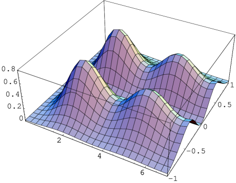
Figure 1: The microscopic spectral density of complex eigenvalues at weak non-Hermiticity parameter $\alpha=0.4$ for $\nu=0$ (left) and $\nu=2$ (right).

It is instructive to look at the density of real eigenvalues $x$ for the chSE [30]

$$\rho_{real}(x)\ =\ 2x^{2}\int_{0}^{1}duu^{2}\int_{0}^{1}dv\left(J_{2\nu}(2uvx)J_{2\nu+1}(2ux)\ -\ vJ_{2\nu}(2ux)J_{2\nu+1}(2uvx)\right)\ .$$ (3.14)

Figure 2: The microscopic spectral density of real eigenvalues for ${\nu=0}$ (left) and ${\nu=2}$ (right).

Compared to the real density the density in the complex plane keeps the oscillatory structure, with the maxima and minima at the same places. However, due to the repulsion of eigenvalues from the real axis the peak structure is doubled, with a valley along the real axis. On the right of Fig. 2 the additional zero eigenvalues at $\nu=2$ repel the density further away from the origin, just as they do in the real case. The double peak structure is very different from the complex chUE [11, 12, 15] and has been detected in lattice simulations [14].

We can also perform an analytical check by taking the limit $\alpha\to 0$ on the microscopic density eq. (3.1). In this limit the pre-factor of the integral becomes

$$\lim_{\alpha\to 0}\frac{1}{32\alpha^{4}}(\xi^{\ast\,2}-\xi^{2})\ |\xi|^{2}\ K_{2\nu}\left(\frac{|\xi|^{2}}{2\alpha^{2}}\right)\mbox{e}^{\frac{1}{4\alpha^{2}}(\xi^{2}+\xi^{*\,2})}\ =\ \frac{i\pi}{16}x\sqrt{x^{2}+y^{2}}\ \delta(y)^{\prime}\ ,$$ (3.15)

where we denote $\xi=x+iy$. Taylor expanding the integrand in the density with respect to $y={\Im\mbox{m}}(\xi)$, we obtain to leading order

$$\lim_{y\to 0}\left(J_{2\nu}(2\sqrt{st}\xi)J_{2\nu}(2\sqrt{s}\xi^{\ast})\ -\ (\xi\leftrightarrow\xi^{\ast})\right)$$

$$=\ 4iy\sqrt{s}\left(J_{2\nu}(2\sqrt{st}x)J_{2\nu+1}(2\sqrt{s}x)-\sqrt{t}J_{2\nu+1}(2\sqrt{st}x)J_{2\nu}(2\sqrt{s}x)\right)\ +\ {\cal O}(y^{2})\ ,$$ (3.16)

after using a Bessel identity. For the limiting spectral density we thus obtain

$$\lim_{\alpha\to 0}\rho_{weak}(\xi) = -\,y\delta(y)^{\prime}\frac{\pi}{4}$$ (3.17)

$$\times x^{2}\int_{0}^{1}ds\int_{0}^{1}dt\sqrt{\frac{s}{t}}\left(J_{2\nu}(2\sqrt{st}\,x)J_{2\nu+1}(2\sqrt{s}\,x)-\sqrt{t}J_{2\nu+1}(2\sqrt{st}\,x)J_{2\nu}(2\sqrt{s}\,x)\right)$$

$$= -\,y\delta(y)^{\prime}\frac{\pi}{2}\rho_{real}(x)\ ,$$

where in the last step we substituted $s=u^{2}$ and $t=v^{2}$. Compared to the Hermitian limit of the chiral complex ensemble [11] the density is not proportional to $\delta(y)$ but to $-y\delta(y)^{\prime}$. This reflects the repulsion from the real axis. Still it gives unity when integrated over the imaginary part $y$, after an integration by parts.

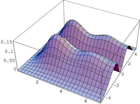
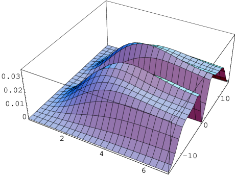
Figure 3: The microscopic spectral density of complex eigenvalues at weak non-Hermiticity parameter $\alpha=1.2$ (left) and $\alpha=2.5$ (right), both for $\nu=0$.

To illustrate our results further we also give the complex density for larger values of the non-Hermiticity parameter $\alpha$. As it is seen in Fig. 3 the oscillations are rapidly damped, with the density starting a to develop a plateau as at strong non-Hermiticity (see Fig. 7). For the latter as well as for an analytic check of this relation by letting $\alpha\to\infty$ we refer to section 4. We also remind the reader that the overall height of the density varies with $\alpha$. This is because of the normalisation to a delta-function in the limit $\alpha\to 0$ eq. (3.15).

3.2 Massive correlation functions at weak non-Hermiticity

After discussing in detail the quenched spectral density we now turn to the presence of massive flavours. We present the spectral density for one pair of degenerate massive flavours $4N_{f}=4$ explicitly, as well as some characteristic polynomials or massive partition functions as examples. Higher order correlation functions and more flavours can then easily be obtained from the given building blocks eq. (3), following the same procedure.

At finite-$N$ the simplest spectral density with non-zero flavour content has $4N_{f}=4$ masses. It is given by

$$R_{N}^{(4)}(z)\ =\ \frac{R_{N+1}^{(0)}(z,im)}{R_{N+1}^{(0)}(im)}\ ,$$ (3.18)

using eq. (2.25). Inserting the explicit expressions eqs. (2.11) and (2.10) we obtain

$$R_{N}^{(4)}(z)\ =\ (z^{*\,2}-z^{2})w(z,z^{*};\tau)\left(\kappa_{N+1}(z,z^{*})\ -\ \frac{|\kappa_{N+1}(z,im)|^{2}-|\kappa_{N+1}(z,-im^{*})|^{2}}{\kappa_{N+1}(im,-im^{*})}\right)\ .$$ (3.19)

While the first term gives exactly the quenched spectral density the second term is a correction term, just as for zero chemical potential [25]. When taking the large-$N$ limit we have to rescale the masses in the same way as the complex eigenvalues in eq. (3.2),

$$\sqrt{2}\ Nm_{f}\ \equiv\ \eta_{f}\ ,\ \ f=1,\ldots,N_{f}\ \ .$$ (3.20)

As we have mentioned at the end of subsection. 2.2, eq. (3.19) includes a limit when setting the masses to be real, $m_{f}=m_{f}^{*}$. This is because of the level repulsions both from the real and imaginary axis: the denominator as well as the numerator of the second term in eq. (3.19) vanishes. The same feature also holds for more general correlation functions eq. (2.25). We illustrate this by Taylor expanding the limiting pre-kernel $\kappa_{weak}(i\eta,-i\eta^{*})$ in the denominator in the imaginary part of the mass $\epsilon\to 0$, setting $\eta=\eta_{x}+i\epsilon$,

$$\lim_{\epsilon\to 0}\kappa_{weak}(i\eta_{x}-\epsilon,-i\eta_{x}-\epsilon)\ =\ \frac{1}{\alpha^{4}}N^{4\nu+4}\frac{2^{2\nu-3}}{(\eta_{x})^{4\nu}}$$

$$\times\ 4i\epsilon\int_{0}^{1}dt\int_{0}^{1}ds\sqrt{\frac{s}{t}}\mbox{e}^{-2s(1+t)\alpha^{2}}\left(\sqrt{t}I_{2\nu+1}(2\sqrt{st}\eta_{x})I_{2\nu}(2\sqrt{s}\eta_{x})-I_{2\nu}(2\sqrt{st}\eta_{x})I_{2\nu+1}(2\sqrt{s}\eta_{x})\right)$$

$$\ +\ {\cal O}(\epsilon^{2})\ .$$ (3.21)

The imaginary argument rotates $J$- to $I$-Bessel functions, where we could have obtained the same result from eq. (3.16), setting $x=i\eta$ and $y=i\epsilon$ there. Making the same expansion for the other terms, $\kappa_{weak}(z,\pm i\eta^{(*)})$ and its conjugates in the numerator, we arrive at the following expression for the microscopic limit of the density eq. (3.19):

$$\rho_{weak}^{(4)}(\xi)\ =\ \rho_{weak}^{(0)}(\xi)\ -\ \Delta\rho_{weak}^{(4)}(\xi)\ \ ,$$ (3.22)

with the first term from eq. (3.1) and the correction term to the quenched density being given by

$$\Delta\rho_{weak}^{(4)}(\xi)\ =\ \frac{1}{32\alpha^{4}}(\xi^{\ast\,2}-\xi^{2})\ |\xi|^{2}\ K_{2\nu}\left(\frac{|\xi|^{2}}{2\alpha^{2}}\right)\exp\left[+\frac{1}{4\alpha^{2}}(\xi^{2}+\xi^{*\,2})\right]$$ (3.23)

$$\times\left\{\left(\int_{0}^{1}\!ds\int_{0}^{1}dt\sqrt{\frac{s}{t}}\ \mbox{e}^{-2s(1+t)\alpha^{2}}(J_{2\nu}(2\sqrt{st}\ \xi)I_{2\nu+1}(2\sqrt{s}\ \eta)-\sqrt{t}I_{2\nu+1}(2\sqrt{st}\ \eta)J_{2\nu}(2\sqrt{s}\ \xi))\right)\right.$$

$$\ \ \left.\times\left(\int_{0}^{1}\!ds\int_{0}^{1}\frac{dt}{\sqrt{t}}\ \mbox{e}^{-2s(1+t)\alpha^{2}}(J_{2\nu}(2\sqrt{st}\,\xi^{*})I_{2\nu}(2\sqrt{s}\,\eta)-I_{2\nu}(2\sqrt{st}\,\eta)J_{2\nu}(2\sqrt{s}\,\xi^{*}))\!\right)-(\xi\leftrightarrow\xi^{*})\right\}$$

$$\times\left[\int_{0}^{1}\!ds\int_{0}^{1}dt\sqrt{\frac{s}{t}}\ \mbox{e}^{-2s(1+t)\alpha^{2}}\left(\sqrt{t}I_{2\nu+1}(2\sqrt{st}\ \eta)I_{2\nu}(2\sqrt{s}\ \eta)-I_{2\nu}(2\sqrt{st}\ \eta)I_{2\nu+1}(2\sqrt{s}\ \eta)\right)\right]^{-1}\!.$$

Here we have again called $\eta_{x}=\eta$ which is now real. Before discussing this main result of the subsection we also briefly give 2 examples for massive partition functions. The simplest case with $2N_{f}=2$ flavours follows from the even skew-orthogonal polynomial at imaginary mass $z=im$, comparing eq. (2.14) and (5):

$${\cal Z}_{N}^{(2N_{f}=2)}(m)/{\cal Z}_{N}^{(0)}=|m|^{2\nu}q_{2N}(im)\ .$$ (3.24)

We can set the mass to be real here without taking limits, as $q_{2N}(im)$ itself does not display any level-repulsion from the axis. We obtain the remarkably simple expression in the weak limit,

$${\cal Z}_{weak}^{(2)}(\eta)\ \sim\ \int_{0}^{1}\frac{dt}{\sqrt{t}}\ \mbox{e}^{-2t\alpha^{2}}I_{2\nu}(2\sqrt{t}\,\eta)\ ,$$ (3.25)

where we have rotated the result eq. (3.8) from the previous subsection to an imaginary argument, skipping all constants (including $N$). As a second example we give the partition function for $4N_{f}=4$ using our formula eq. (LABEL:Zmrho),

$${\cal Z}_{N}^{(4)}(m)/{\cal Z}_{N+1}^{(0)}\ =\ \frac{|m|^{4\nu}}{(N+1)}\frac{\kappa_{N}(im,-im^{*})}{(m^{2}-m^{*\,2})}\ .$$ (3.26)

Upon using the same expansion as for the density eq. (3.21) we immediately obtain

$${\cal Z}_{weak}^{(4)}(\eta)\sim\frac{1}{\eta\alpha^{4}}\int_{0}^{1}\!dt\int_{0}^{1}\!ds\sqrt{\frac{s}{t}}\,\mbox{e}^{-2s(1+t)\alpha^{2}}\!\left(\sqrt{t}I_{2\nu+1}(2\sqrt{st}\eta)I_{2\nu}(2\sqrt{s}\eta)-I_{2\nu}(2\sqrt{st}\eta)I_{2\nu+1}(2\sqrt{s}\eta)\right),$$ (3.27)

where we have again suppressed all constants. Due to the presence of conjugate pairs of complex eigenvalues the dependence on $\alpha$ cannot be factored out, similar to the same situation in the unitary ensembles [27, 12, 16]. Such a simplification only occurs in the absence of conjugate flavours, in the QCD matrix model with a sign problem [31, 15, 16], where the partition function can be normalised to be $\mu$-independent. As a check both expressions eqs. (3.25) and (3.27) reduce to the know results [32, 25] in the limit $\alpha\to 0$.

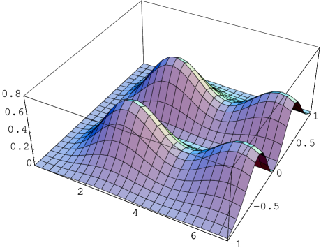
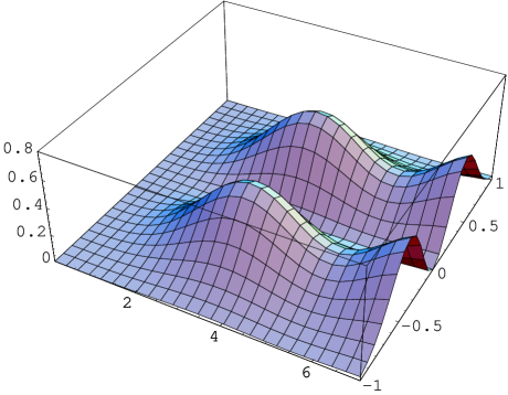
Figure 4: The massive microscopic spectral density at weak non-Hermiticity parameter $\alpha=0.4$ for masses $\eta=8.74$ (left) and $\eta=4.26$ (right), both at $\nu=0$.

Figure 5: The massive microscopic spectral density of real eigenvalues for masses $\eta=8.74$ (left) and $\eta=4.26$ (right), both at ${\nu=0}$.

Let us now discuss the massive density eq. (3.22). In Fig. 5 we plot the microscopic, massive spectral density for two different values of masses $\eta=8.74$ and $\eta=4.26$, both at weak non-Hermiticity parameter $\alpha=0.4$ and $\nu=0$, and compare it the corresponding expression for real eigenvalues [25]. We have deliberately chosen the same values for the mass parameter as there, where numerical data for lattice simulations with dynamical fermions at $\mu=0$ [33] were compared. Similar to having $\nu=2$ exact zero eigenvalues in Fig. 1 the eigenvalues are pushed further away from the origin through the masses. Below we compare the corresponding expression for real eigenvalues at the same values of the mass parameters [25]. As for the quenched case the correlation functions keep their oscillatory structure, with the maxima located at the same positions as for real eigenvalues, at the given value of $\alpha$.

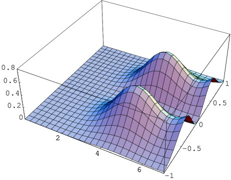
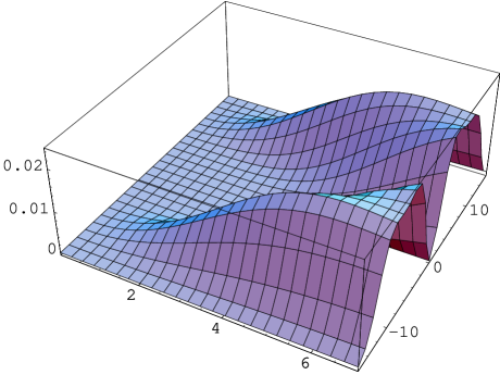
Figure 6: The massive microscopic spectral density at weak non-Hermiticity parameter at $\alpha=0.4$ with mass $\eta=1$ (left) and at $\alpha=2.5$ with $\eta=4.26$ (right), both at $\nu=0$.

Furthermore we observe that for larger masses the density moves toward the quenched density in Fig. 1, as the infinite mass limit quenches the fermion determinant. On the other hand smaller masses moving towards the origin push the eigenvalues further out. In the zero-mass limit the density should approach the quenched density at topological charge $\nu=2$ approximately, as can be seen in Fig. 5 left. Although for non-zero chemical potential there is no more flavour-topology duality [34] because of the explicit $\nu$-dependence in the $K$-Bessel functions in the weight, this duality holds approximately, when the $K$-Bessel function reaches its asymptotic, $\nu$-independent form. For those values of $|\xi^{2}|/(2\alpha^{2})$ in Fig. 6 left, where the density is non-vanishing, this is indeed the case.

As a final example we display the massive density at a larger value of $\alpha=2.5$ in Fig. 6 right. As seen already for the quenched density the oscillations are washed out (compared to Fig. 5 right). A further feature can be seen here. For the chosen value of $\alpha$ and $\eta$ the $\xi$-value where the mass factor $|\xi^{2}+\eta^{2}|^{2}$ vanishes, $\pm{\Im\mbox{m}}(\xi)=\eta$, now lies on the imaginary axis inside the shown picture. It can be seen very clearly that the eigenvalues are pushed away from the very location of the mass, in addition to the level repulsion from the $y$-axis.

In the previous subsection we performed an analytical check by taking the Hermitian limit $\alpha\to 0$ of the spectral density and comparing it to the known expression for the density of real eigenvalues. We have performed the same check here where we refer to [25] for the corresponding expression for the massive spectral density of real eigenvalues. Without going through the details we just comment of the structure to be obtained.

Since our example eq. (3.18) involves the two-point function it contains all four elements of the matrix kernel eq. (2.8), the pre-kernel $\kappa_{N}$ at different (complex conjugated arguments). In contrast to that for real eigenvalues the two-point or higher correlation functions are given by a quaternion determinant of a two by two matrix kernel with different matrix elements: a pre-kernel which is basically given by eq. (3.14), its derivative and its integral (see [30]). How can we obtain these three different matrix elements from one pre-kernel? Taking the limit $\alpha\to 0$ invokes a further derivative with respect to the imaginary part $y={\Im\mbox{m}}(\xi)$, in addition to the expansion in eq. (3.23) due to real masses. As a result we will get the real limit of the pre-kernel eq. (3), its first and second derivative, correctly reproducing all terms in [25] for the real massive density.

4 The strong non-Hermiticity limit

The regime of strong non-Hermiticity in defined by taking the limit $N\to\infty$ while keeping $\mu\in(0,1]$ fixed. The rescaling of the eigenvalues is modified compared to eq. (3.2), keeping

$$\sqrt{N}\ ({\Re\mbox{e}}\ z+i{\Im\mbox{m}}\ z)\ =\ \sqrt{N}\ z\ \equiv\xi\ \ \$$ (4.1)

finite. Hence the definition of the large-$N$ correlation functions is also altered, reading

$$\kappa_{strong}(\xi_{1},\xi_{2}^{\ast}) \equiv \lim_{N\to\infty}\frac{1}{N}\ \kappa_{N}\left(\frac{\xi_{1}}{\sqrt{N}},\frac{\xi_{2}^{\ast}}{\sqrt{N}}\right),$$

$$\rho_{strong}(\xi_{1},\ldots,\xi_{k}) \equiv \lim_{N\to\infty}\frac{1}{N^{k}}\ R_{N}\left(\frac{\xi_{1}}{\sqrt{N}},\ldots,\frac{\xi_{k}}{\sqrt{N}}\right).$$ (4.2)

The difference in scaling can be easily understood as follows. At weak non-Hermiticity the eigenvalues remain close to the real axis, with their imaginary part being small compared to the real part. In order to obtain a macroscopic density at the origin of the order $\rho_{macro}(0)\sim N$ their average distance has to be ${\cal O}(1/N)$. In contrast to that at strong non-Hermiticity the eigenvalues spread out in the complex plane, having a comparable real and imaginary part. To form again a constant macroscopic density $\rho_{macro}(0)\sim N$ the average distance between nearest neighbours has to be ${\cal O}(1/N^{2})$. Here we measure distance with respect to the two-dimensional metric.

A clear separation of scales between the two different limits can be defined as follows. At weak non-Hermiticity the microscopic density describes the universal fall off to zero of the eigenvalues away from the imaginary axis. In direction of the real axis along the maxima we obtain as usual $\lim_{\Re ez\to\infty}\rho_{weak}(z)=\rho_{macro}(0)$ . In contrast to that at strong non-Hermiticity the microscopic density attains the constant value of the macroscopic one in all directions, $\lim_{|z|\to\infty}\rho_{strong}(z)=\rho_{macro}(0)$, as can be seen below in Figs. 7 and 8. This is of course except along the real and imaginary axis, due to the repulsion from the Jacobian in eq. (2.4). The fall-off of the macroscopic density to zero in any direction (which is not seen in the microscopic regime here) can then be expected to be given by another microscopic function at the edge, in analogy to the Airy-kernel for real ensembles at the edge of the spectrum. When numerically solving the matrix model at finite but large-$N$ care has to be taken to ensure a clear separation between micro- and macroscopic density when comparing to the analytic formulas.

The computation of correlation functions at strong non-Hermiticity is more involved, as is already the case in the non-chiral ensemble [19]. In fact we will follow the same strategy as there, by first deriving a differential equation for the large-$N$ pre-kernel at maximal non-Hermiticity $\mu=1$. A solution of this equation can be obtained either directly or by taking the limit $\alpha\to\infty$ of the pre-kernel at weak non-Hermiticity, keeping $\xi_{weak}/\alpha$ fixed. Since the two methods match it is suggestive to recover the full range of strong non-Hermiticity $\mu\in(0,1]$ by inserting a $\mu$-dependent parameter through $\xi\to\xi\Sigma(\mu)$. However, we can also argue that such a rescaling can always be absorbed by redefining the scaling limit eq. (4.1). Details of the derivation of the differential equation and its solution are given in the appendix B.

We begin by taking the limit of maximal non-Hermiticity $\mu\to 1$ on the skew orthogonal polynomials eqs. (2.28) and (LABEL:qeven). In this limit only the highest powers survive and they become monic or a sum over monomials, respectively. We thus obtain the following expression for the pre-kernel eq. (2.9) in the microscopic large-$N$ limit eq. (4.2):

$$\left.\kappa_{strong}(\xi,\zeta^{*})\right|_{\mu=1}\ =\ \frac{N^{2\nu+2}}{\pi 2^{2\nu+3}}\sum_{k=0}^{\infty}\sum_{j=0}^{k}\frac{k!\Gamma(k+\nu+1)}{\Gamma(2k+2\nu+2)(2k+1)!}\frac{(\xi^{4k+2}\zeta^{*\,4j}\ -\ \xi^{4j}\zeta^{*\,4k+2})}{2^{4j}j!\Gamma(j+\nu+1)}\ .$$ (4.3)

It can be shown that the function $\kappa_{strong}(\xi,\zeta^{*})$ obeys the following set of inhomogeneous second order differential equations

$$\frac{1}{2}\left[\partial_{\xi}^{2}+\frac{(4\nu+1)}{\xi}\partial_{\xi}-\xi^{2}\right]\kappa_{strong}(\xi,\zeta^{*})|_{\mu=1} = +\ \frac{N^{2\nu+2}}{4\pi}\frac{I_{2\nu}\left(\xi\zeta^{*}\right)}{(\xi\zeta^{*})^{2\nu}}\ ,$$

$$\frac{1}{2}\left[\partial_{\zeta^{*}}^{2}+\frac{(4\nu+1)}{\zeta^{*}}\partial_{\zeta^{*}}-\zeta^{*\,2}\right]\kappa_{strong}(\xi,\zeta^{*})|_{\mu=1} = -\ \frac{N^{2\nu+2}}{4\pi}\frac{I_{2\nu}\left(\xi\zeta^{*}\right)}{(\xi\zeta^{*})^{2\nu}}\ ,$$ (4.4)

where we refer to the appendix B for details. Due to the antisymmetry of the pre-kernel the right hand side changes sign. The solution of this equation can be constructed as explained in the appendix B. The result is given by

$$\kappa_{strong}(\xi,\zeta^{*})|_{\mu=1} = \frac{N^{2\nu+2}}{2\pi}\frac{1}{(\xi\zeta^{*})^{2\nu}}\mbox{e}^{\frac{1}{2}(\xi^{2}+\zeta^{*\,2})}$$ (4.5)

$$\times\int_{0}^{\infty}dq\int_{0}^{q}dp\,\mbox{e}^{-q^{2}-p^{2}}\left[J_{2\nu}(2q\zeta^{*})J_{2\nu}(2p\xi)\ -\ J_{2\nu}(2q\xi)J_{2\nu}(2p\zeta^{*})\right]\ .$$

In order to obtain all correlation functions from eq. (4.5) we next give the weight function eq. (2.26) in the limit of strong non-Hermiticity eq. (4.1):

$$w_{K}^{(2\nu)}(\xi,\xi^{*})\ =\ N^{-2\nu-1}|\xi|^{4\nu+2}K_{2\nu}\left(\frac{(1+\mu^{2})|\xi|^{2}}{2\mu^{2}}\right)\exp\left[\frac{1-\mu^{2}}{4\mu^{2}}(\xi^{2}+\xi^{*\,2})\right]\ ,\ \ \mu\in\,(0,1]\ .$$ (4.6)

Here we display the weight for any value of the strong non-Hermiticity $\mu$. At $\mu=1$ the expression simplifies, the exponential factor cancels with the kernel and the argument inside the $K$-Bessel function reduces to unity times $|\xi|^{2}$. Inserting this into eq. (2.10) we obtain the following result for the microscopic spectral density at maximal non-Hermiticity

$$\rho_{strong}(\xi)|_{\mu=1} = \frac{1}{2\pi}(\xi^{\ast\,2}-\xi^{2})|\xi|^{2}K_{2\nu}\left({|\xi|^{2}}\right)\mbox{e}^{\frac{1}{2}(\xi^{2}+\xi^{*\,2})}$$

$$\times \int_{0}^{\infty}dq\int_{0}^{q}dp\ \mbox{e}^{-q^{2}-p^{2}}\left[J_{2\nu}\left({2q\xi^{\ast}}\right)J_{2\nu}\left({2p\xi}\right)\ -\ J_{2\nu}\left({2q\xi}\right)J_{2\nu}\left({2p\xi^{\ast}}\right)\right]\ .$$

As an analytic check we have performed the limit $\alpha\to\infty$ of the microscopic spectral density at weak non-Hermiticity eq. (3.1), where we refer to the end of appendix B for details. We obtain exactly the same functional form of the spectral density, eq. (B.2) (up to a different constant normalisation), in terms of the variable $\xi_{S}=\sqrt{N}\,z/\mu\sqrt{2}$.

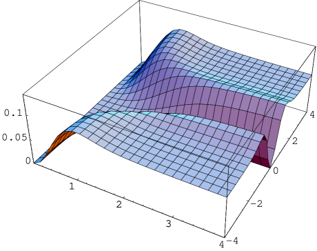
Figure 7: The microscopic spectral density at maximal non-Hermiticity $\mu=1$ with $\nu=0$ (left) and $\nu=2$ (right) .

Together with eq. (4.6) this leads us to conjecture that the $\mu$-dependence at strong non-Hermiticity with $\mu<1$ can be restored as follows, replacing

$$\xi^{2}\ \longrightarrow\ \frac{(1+\mu^{2})}{2\mu^{2}}\xi^{2}$$ (4.8)

everywhere in eq. (4). We have shown it to be true for $\mu=1$ and for small $\mu\ll 1$. However, if this is true we could then redefine our strong non-Hermiticity limit eq. (4.1) to completely reabsorb this $\mu$-dependence, defining

$$\frac{\sqrt{1+\mu^{2}}}{\mu\sqrt{2}}\sqrt{N}\ z\ \equiv \xi$$ (4.9)

$$\rho_{strong}(\xi_{1},\ldots,\xi_{k}) \equiv \lim_{N\to\infty}\frac{2^{k}\mu^{2k}}{(1+\mu^{2})^{k}N^{k}}\ R_{N}\left(\frac{\xi_{1}\mu\sqrt{2}}{\sqrt{(1+\mu^{2})N}},\ldots,\frac{\xi_{k}\mu\sqrt{2}}{\sqrt{(1+\mu^{2})N}}\right).$$

As an illustration of our results we show the microscopic spectral density eq. (4) and its dependence on $\nu$ at maximal non-Hermiticity $\mu=1$ in Fig. 7. One can clearly see that for $\nu=2$ the additional zero eigenvalues push the density away from the origin. For the numerically evaluation of the integral in eq. (4) necessary to plot it an equivalent representation of the integral is very convenient. Using the identity derived in the appendix eq. (B.23) we have

$$\rho_{strong}(\xi)\ =\ \frac{1}{4\pi}(\xi^{\ast\,2}-\xi^{2})|\xi|^{2}K_{2\nu}\left({|\xi|^{2}}\right)\int_{0}^{1}\frac{dr}{\sqrt{1-r^{2}}}\ I_{2\nu}(r|\xi|^{2})\sinh\left(\frac{1}{2}\sqrt{1-r^{2}}\,(\xi^{2}-\xi^{\ast\,2})\right),$$ (4.10)

where the exponential pre-factor has cancelled out. This form of the density allows to dicuss its rotation and reflection symmetries most clearly.

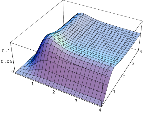
Figure 8: Part of Fig. 7 (left) showing the first quadrant only. The symmetry with respect to the diagonal ${\Re\mbox{e}}\xi={\Im\mbox{m}}\xi$ is clearly visible .

The fact that it is an even function of $(\xi^{2}-\xi^{\ast\,2})$ and otherwise only depends on the modulus $|\xi|^{2}$ leads to the following properties. First, one can obviously rotate the density by $\pi/2$, $\pi$, or $3\pi/2$, multiplying $\xi$ by $i$ , $(-1)$, or $-i$ without changing it. Second, the density is invariant under reflections along the $x$-, $y$-, $(x=y)$- and $(x=-y)$-axis where $\xi=x+iy$. For example for the $(x=y)$-axis in the first quadrant we write the pair of $\xi$-values related by reflection as

$$\xi_{\pm}\equiv r\mbox{e}^{i\frac{\pi}{4}\,\pm i\delta}\ \ \Rightarrow\ \ \xi_{\pm}^{*}=-i\xi_{\mp}.$$ (4.11)

The modulus remains unchanged, $|\xi_{+}|=|\xi_{-}|$, as well as the difference $(\xi_{+}^{2}-\xi_{+}^{\ast\,2})=-(\xi_{-}^{*\,2}-\xi_{-}^{2})$. This symmetry can be observed in Fig. 8. The remaining reflection symmetries easily follow in a similar way.

4.1 Massive correlation functions at strong non-Hermiticity

In this subsection we give the simplest nontrivial result including one pair of degenerate massive flavours, $4N_{f}=4$, where we will follow closely the corresponding subsection 3.2 at weak non-Hermiticity. Higher order correlations as well as more flavours follow along the same lines. We start by defining how to rescale the masses

$$\sqrt{N}\,m_{f}\ \equiv\ \eta_{f}\ ,\ \ f=1,\ldots,N_{f}\ ,$$ (4.12)

in analogy to the eigenvalues in eq. (4.1). In order to derive the massive spectral density we could simply take the limit $\alpha\to\infty$ of the expressions in eqs. (3.1) and (3.23) at weak non-Hermiticity, together with the results from appendix B.

In order to give more compact expressions we derive results using the alternative form of the strong density eq. (4.10) and the corresponding kernel. The massive spectral density follows again from eq. (3.19) at finite-$N$. The kernel at strong non-Hermiticity we use is obtained from eq. (4.5) by inserting eq. (B.23):

$$\kappa_{strong}(\xi,\zeta^{*})\ =\ \frac{N^{2\nu+2}}{4\pi}\frac{1}{(\xi\zeta^{*})^{2\nu}}\int_{0}^{1}dr\frac{1}{\sqrt{1-r^{2}}}\,I_{2\nu}(r\xi_{S}\zeta_{S}^{*})\sinh\left(\frac{1}{2}\sqrt{1-r^{2}}\,(\xi_{S}^{2}-\zeta_{S}^{*\,2})\right).$$ (4.13)

Expanding again in the imaginary part of the mass $\epsilon\to 0$, setting $\eta=\eta_{x}+i\epsilon$ we easily obtain for the denominator of eq. (3.19)

$$\lim_{\epsilon\to 0}\kappa_{strong}(i\eta_{x}-\epsilon,-i\eta_{x}-\epsilon)\ =\ \frac{N^{2\nu+2}}{4\pi}\frac{1}{(\eta_{x})^{4\nu}}(-2i)\,\epsilon\,\eta_{x}\int_{0}^{1}drI_{2\nu}(r\eta_{x}^{2})\ +\ {\cal O}(\epsilon^{2})\ .$$ (4.14)

The same expansion can be done for $\kappa_{strong}(\xi,\pm\eta^{(*)})$ and its conjugates, leading to the following expression for the massive spectral density at strong non-Hermiticity:

$$\rho_{strong}^{(4)}(\xi)\ =\ \rho_{strong}^{(0)}(\xi)\ -\ \Delta\rho_{strong}^{(4)}(\xi)\ ,$$ (4.15)

with the quenched density given by eq. (4.10). The correction term reads

$$\Delta\rho_{strong}^{(4)}(\xi)\ =\ -\frac{1}{4\pi}(\xi^{\ast\,2}-\xi^{2})|\xi|^{2}K_{2\nu}\left({|\xi|^{2}}\right)\left\{\int_{0}^{1}\frac{dr}{\sqrt{1-r^{2}}}J_{2\nu}(r\xi\eta)\sinh[\frac{1}{2}\sqrt{1-r^{2}}\,(\xi^{2}+\eta^{2})]\right.$$

$$\times\left(\int_{0}^{1}\!\!\!\!\frac{dr\,r\xi^{*}}{\sqrt{1-r^{2}}}J_{2\nu+1}(r\xi^{*}\eta)\sinh[\frac{1}{2}\sqrt{1-r^{2}}(\xi^{*\,2}+\eta^{2})]-\!\!\int_{0}^{1}\!\!\!\!dr\eta J_{2\nu}(r\xi^{*}\eta)\cosh[\frac{1}{2}\sqrt{1-r^{2}}(\xi^{*\,2}+\eta^{2})]\!\right)$$

$$\ \ \ \ -\ (\xi\leftrightarrow\xi^{*})\left\}\times\left[\eta\int_{0}^{1}dr\ I_{2\nu}(r\eta^{2})\right.\right]^{-1}\!.$$ (4.16)

We have again called $\eta=\eta_{x}$ which is now real. Before discussing the massive spectral density let us also give some examples for partition functions. Taking the strong non-Hermiticity limit of eq. (3.26) at $4N_{f}=4$ we simply have to insert the expansion eq. (4.14) to obtain

$${\cal Z}_{strong}^{(4)}(\eta)\ \sim\ \int_{0}^{1}drI_{2\nu}(r\eta^{2})\ ,$$ (4.17)

up to suitable normalisation constants. Since we did not compute the asymptotic even skew-orthogonal polynomials at generic strong non-Hermiticity $0<\mu\leq 1$ we cannot directly use eq. (3.24) for $2N_{f}=2$. We can circumvent this problem by taking the infinite $\alpha$ limit on eq. (3.25), leading to the following

$${\cal Z}_{strong}^{(2)}(\eta)\ =\ \lim_{\alpha\to\infty}{\cal Z}_{weak}^{(2)}(\eta=\eta_{w}/\alpha\sqrt{2})\ \sim\ \mbox{e}^{\frac{\eta^{2}}{2}}I_{\nu}\left(\frac{\eta^{2}}{2}\right)\ .$$ (4.18)

Let us come back to the spectral density eq. (4.16). Below we show a few examples for the influence of the mass parameter at maximally strong non-Hermiticity.

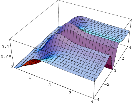
Figure 9: The massive spectral density at at mass $\eta=2.5$ with $\nu=0$ (left) and $\nu=2$ (right) .

Compared to the quenched density in Fig. 7 left there is an additional level repulsion from the mass, when $\pm{\Im\mbox{m}}(\xi)=\eta$. Non-zero topology leads to an additional level repulsion from the origin as can be seen in Fig. 9 right, and both the effects of mass and $\nu$ can be clearly separated (see also Fig. 7 right).

For smaller values of the mass parameter the density approaches approximatively the quenched density at $\nu=2$, as the mass acts as additional zero eigenvalues (comparing Fig. 10 left and Fig. 7 right). On the other hand going to larger masses we get back the quenched density as can be seen in Fig. 10 right.

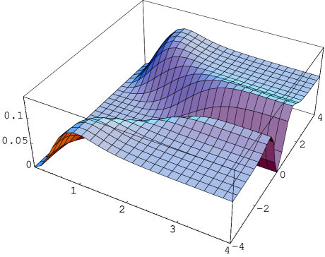
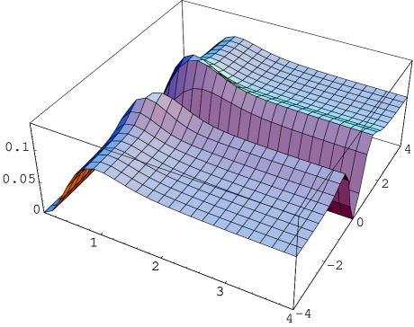
Figure 10: The massive spectral density at at mass $\eta=0.5$ (left) and $\eta=8$ (right), both with $\nu=0$ .

Of course there is still level repulsion at the large mass value, in this case $\eta=8$, as displayed in Fig. 11. However, this does no longer affect the density at the origin. Furthermore, there are no strong oscillations observed here at the location of the mass, as seen in unquenched QCD [16]. Here, the situation is very similar to phase quenched QCD also reported in [16] on the matrix model in the $\beta=2$ symmetry class. These findings underline once more the importance of the presence or absence of the sign problem on the level of the microscopic complex eigenvalue correlations of the Dirac operator.

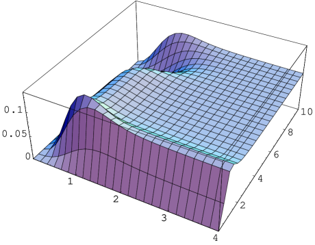
Figure 11: Part of Fig. 10 (right) showing the first quadrant for a larger argument ${\Im\mbox{m}}(\xi)$. The level repulsion at the mass value $\xi=8i$ is clearly visible.

We note in passing that because of the analytic relationship between the correlations at strong non-Hermiticity and weak non-Hermiticity at large $\alpha$ similar figures could have obtained in this section by plotting the corresponding pictures at large enough $\alpha$. We have checked this numerically in several cases for both the quenched and massive density, with $\alpha=5$ (see also Fig. 6). However, such a density at weak non-Hermiticity will always vanish for large enough $\pm{\Im\mbox{m}}(\xi)$, at any given $\alpha$. In contrast to that the density at strong non-Hermiticity remains constant.

5 Relation to the Dirac operator spectrum with chemical potential

The purpose of this section is twofold. First, we give a more detailed discussion of the matrix representation of our complex eigenvalue model eq. (2.4) in terms of two non-Hermitian quaternion real matrices, including mass terms. This justifies to speak of a matrix model ensemble. It also gives an explicit realization of the joint probability distribution in eq. (2.4) by computing the Jacobian that leads to complex eigenvalues. In particular it yields the special weight function eq. (2.26) containing a $K$-Bessel function. The second purpose is to relate the model to the Dirac operator spectrum of QCD-like gauge theories in the presence of a chemical potential. To do this matching we need to compare the global symmetries of such Dirac operators to a random matrix representation.

The Dirac operator as it appears in four dimensional gauge theories can be represented by an anti-Hermitian block matrix, $\hbox to0.0pt{ $\,\raisebox{0.6458pt}{/}\hss$}D_{gauge}=\left(\begin{array}[]{cc}0&iW\\ iW^{\dagger}&0\\ \end{array}\right)$, with non vanishing entries only on the off diagonal due to chiral symmetry. For different gauge groups and representations the off-diagonal blocks $W$ have either a orthogonal, unitary, or symplectic symmetry, as was pointed out in [9]. Adding a chemical potential $\mu$ for the quarks amounts to shifting the Dirac operator by $\hbox to0.0pt{ $\,\raisebox{0.6458pt}{/}\hss$}D_{gauge}\to\hbox to0.0pt{ $\,\raisebox{0.6458pt}{/}\hss$}D_{gauge}+\mu\gamma_{0}$ where $\gamma_{0}$ is a Dirac-$\gamma$ matrix. In a given basis it is represented as a block matrix as well, with unit elements on the off diagonals only [2]. Being Hermitian this addition destroys the anti-Hermiticity property, where the sum $\hbox to0.0pt{ $\,\raisebox{0.6458pt}{/}\hss$}D_{gauge}+\mu\gamma_{0}$ now has complex eigenvalues. The generalisation of the classification [9] to $\mu\neq 0$ we use here was made in [10].

If we replace the Dirac operator by a random matrix we have to satisfy two criteria. First, $\hbox to0.0pt{ $\,\raisebox{0.6458pt}{/}\hss$}D_{gauge}$ may have exact zero eigenvalues corresponding to different sectors of topological charge through an index theorem. For a fixed number $\nu$ of zero modes, which we shall always consider here, we thus have to replace the blocks $W$ by rectangular matrices, of size $(N+\nu)\times N$. Second and more importantly, these rectangular matrices have to be in the same symmetry class as the corresponding gauge theory, consisting of real, complex or quaternion real elements [9, 10]. The latter case which we consider here, also labelled by the Dyson index $\beta=4$, describes $SU(N_{c})$ gauge theories in the adjoint representation. When representing the gauge theory on a lattice using staggered fermions the corresponding symmetry is an $SU(N_{c}=2)$ gauge theory in the fundamental representation.

The addition of a chemical potential in the matrix model can be done in different ways. It was first suggested [2, 10] to add it as a constant times $\gamma_{0}$, the off diagonal unity matrix, assuming this term to be diagonal in the random matrix space. While this model successfully explained the failure of the quenched approximation [2] an analytical treatment of all complex eigenvalue correlations from orthogonal polynomials similar to the $\mu=0$ case was not achieved to date, apart from the quenched spectral density obtained using the replica method [12]. Therefore a different matrix model representation of the chemical potential term was suggested very recently in [15] for the QCD symmetry class $\beta=2$. It assumes that the chemical potential term is non-diagonal in matrix space and is represented by a second, uncorrelated matrix which has the same symmetries as the one modelling the $\mu=0$ part. Making the model more complicated at first sight it has the remarkable feature of leading to a complex eigenvalue representation, which then allows for a treatment using (bi-)orthogonal polynomials [15, 16]. A different model given only in terms of complex eigenvalues was first suggested in [11] and tested in quenched QCD lattice simulations [13]. Although it is lacking the matrix symmetries of $\hbox to0.0pt{ $\,\raisebox{0.6458pt}{/}\hss$}D_{gauge}$ it asymptotically agrees with the results of [12, 15] (see the weight eq. (2.27) vs. eq. (2.26)).

In the following we will adopt the strategy of [15] and apply it to the complex $\beta=4$ symmetry class. Our corresponding matrix model is thus given in terms of two rectangular $(N+\nu)\times N$ matrices, $\Phi$ and $\Psi$, with quaternion real elements without further symmetry properties:

$${\cal Z}_{N}^{(2N_{f})}(\{m_{f}\})\equiv\int d\Phi d\Psi\exp\left[-N{\mbox{Tr}}(\Phi^{\dagger}\Phi\ +\ \Psi^{\dagger}\Psi)\right]\prod_{f=1}^{N_{f}}\det\left(\begin{array}[]{cc}m_{f}\mbox{\bf 1}&i\Phi+\mu\Psi\\ i\Phi^{\dagger}+\mu\Psi^{\dagger}&m_{f}\mbox{\bf 1}\end{array}\right),$$ (5.1)

where 1 is the quaternion unity element. Compared to eq. (2.1) we have now included the quark masses. As a first step we define the linear combinations

$$C \equiv i\Phi\ +\mu\Psi$$

$$D \equiv i\Phi^{\dagger}+\mu\Psi^{\dagger}\ ,$$ (5.2)

with a trivial constant Jacobian. In terms of these new matrices the partition function reads

$${\cal Z}_{N}^{(2N_{f})}(\{m_{f}\}) \sim \int dCdD\exp\left[-N\frac{(1+\mu^{2})}{4\mu^{2}}{\mbox{Tr}}(C^{\dagger}C+DD^{\dagger})-N\frac{(1-\mu^{2})}{4\mu^{2}}{\mbox{Tr}}(DC+C^{\dagger}D^{\dagger})\right]$$ (5.5)

$$\times\prod_{f=1}^{N_{f}}\det\left(\begin{array}[]{cc}m_{f}\mbox{\bf 1}&C\\ D&m_{f}\mbox{\bf 1}\end{array}\right).$$

In this form we have only convergent integrals for $\mu\in\ [0,1]$ at finite-$N$, as can be seen from eq. (5) below. We will not discuss the possibility of phase transitions here, where for lattice simulations of this situation we refer to [35].

The Dirac matrix inside the determinant has $\nu$ zero eigenvalues and $N$ complex eigenvalues which come in pairs of opposite sign as well as complex conjugate pairs. The former is due to chiral symmetry and the latter is due to the symplectic structure as the eigenvalues of a quaternion real matrix come in complex conjugate pairs. It is this symplectic structure that is responsible for the fact that the determinant will remain positive definite, without having a sign problem as unquenched QCD. It makes this symmetry class an ideal testing ground for lattice simulations with dynamical fermions in the presence of a chemical potential.

In the next step we parametrise the matrices $C$ and $D$ as follows,

$$C = U(X+R)V$$

$$D = V^{\dagger}(Y+S)U^{\dagger}\ ,$$ (5.6)

which is equivalent to making an independent Schur decomposition of $CD$ and $DC$. Here $U$ and $V$ are symplectic matrices. The matrices $R$ and $S$ are upper triangular with real quaternion elements, and we have split off their diagonal parts $X$ and $Y$ which are also quaternion real, without containing the second and third quaternion unit (see e.g. [17] for explicit representations). They contain the complex eigenvalues of $C$ and $D$ which come in $N$ pairs $(x_{k},x_{k}^{*})$ for the matrix $X$ and $(y_{k},y_{k}^{*})$ for the matrix $Y$ respectively. The parametrisation is not unique as under an additional diagonal unitary transformation the matrices remain triangular. It only changes the upper triangular matrices $R$ and $S$ which we will integrate out afterwards. This symmetry can be used to restrict the matrices to be $V\in\ Sp(N)/U(1)^{N}$ and $U\in\ Sp(N+\nu)/(Sp(\nu)\times U(1)^{N})$. The parametrisation eq. (5.6) as well as the counting of degrees of freedom is discussed most explicitly in appendix C. The relation to the original eigenvalues of the Dirac matrix is

$$x_{k}y_{k}\ =\ -z_{k}^{2}\ ,$$ (5.7)

which explains that the eigenvalues of $CD$ come in complex conjugate pairs $(z_{k}^{2},z_{k}^{*\,2})$, $k=1,\ldots N$. The final Jacobian of the transformation computed in appendix C reads

$$\det\left(\frac{\partial(C,D)}{\partial(X,Y,U,V,R,S)}\right)\ =\ \prod_{j}^{N}|x_{j}|^{4\nu}\prod_{k>l}^{N}|z_{k}^{2}-z_{l}^{2}|^{2}\ |z_{k}^{2}-z_{l}^{\ast\,2}|^{2}\prod_{h=1}^{N}|z_{h}^{2}-z_{h}^{\ast\,2}|^{2}\ ,$$ (5.8)

after a suitable ordering of the independent variables. We can now integrate out the symplectic matrices $U$ and $V$, as well as the Gaussian integrals over $R$ and $S$ to obtain

$${\cal Z}^{(2N_{f})}_{N}(\{m_{f}\}) \sim \int\prod_{j=1}^{N}d^{2}x_{j}\,d^{2}y_{j}\exp\left[-N\frac{(1+\mu^{2})}{4\mu^{2}}(|x_{j}|^{2}+|y_{j}|^{2})+N\frac{(1-\mu^{2})}{4\mu^{2}}(z_{j}^{2}+z_{j}^{*\,2})\right]$$ (5.9)

$$\times|x_{j}|^{4\nu}\prod_{f=1}^{N_{f}}|m_{f}|^{2\nu}|z_{j}^{2}+m_{f}^{2}|^{2}\prod_{k>l}^{N}|z_{k}^{2}-z_{l}^{2}|^{2}\ |z_{k}^{2}-z_{l}^{\ast\,2}|^{2}\prod_{h=1}^{N}|z_{h}^{2}-z_{h}^{\ast\,2}|^{2}\ .$$

Here we have included the mass dependent factor $\sim|m_{f}|^{2\nu}$ in the normalisation, to the power of mass degeneracy 2 in $2N_{f}$. Although we have now achieved an eigenvalues representation in terms of $x_{k}$ and $y_{k}$ we still have twice as many degrees of freedom that what we aimed at, a single set of $N$ complex eigenvalues $z_{k}$. If we substitute $y_{k}$ by $z_{k}$: $y_{k}=-z_{k}^{2}/x_{k}$ we can integrate out the variables $x_{k}$ in analogy to [15], after decomposing them into polar coordinates,

$${\cal Z}^{(2N_{f})}_{N}(\{m_{f}\}) \sim \int\prod_{j=1}^{N}d^{2}z_{j}\ K_{2\nu}\!\left(\frac{N(1+\mu^{2})}{2\mu^{2}}|z_{j}|^{2}\right)\exp\left[\frac{N(1-\mu^{2})}{4\mu^{2}}(z_{j}^{2}+z_{j}^{*\,2})\right]$$

$$\times|z_{j}|^{4\nu+2}\prod_{f=1}^{N_{f}}|m_{f}|^{2\nu}|z_{j}^{2}+m_{f}^{2}|^{2}\prod_{k>l}^{N}|z_{k}^{2}-z_{l}^{2}|^{2}\ |z_{k}^{2}-z_{l}^{\ast\,2}|^{2}\prod_{h=1}^{N}|z_{h}^{2}-z_{h}^{\ast\,2}|^{2}$$

$$\sim \left\langle\prod_{f=1}^{N_{f}}\det\left(\begin{array}[]{cc}m_{f}&C\\ D&m_{f}\end{array}\right)\right\rangle_{{\cal Z}^{(0)}_{N}}.$$ (5.13)

This gives us a complex eigenvalue model as in eq. (2.4) with the specific weight function eq. (2.26) plus mass terms, as well as a matrix representation of the $q_{2N}(z)$ eq. (2.14) for $N_{f}=1$. We note that compared to the QCD symmetry class [15] the index of the $K$-Bessel function is shifted: $\nu\to 2\nu$. The massive partition functions eq.(2.16) computed in section 2.2 are obtained by taking $4N_{f}$ flavours of twofold degenerate real masses $m_{f}$ in eq. (5.1), or $2N_{f}$ flavour pairs of complex conjugate masses $(m_{f},m_{f}^{*})$ for complex masses:

$${\cal Z}^{(4N_{f})}_{N}(\{m_{f}\})\ \sim\ \left\langle\prod_{f=1}^{N_{f}}\det\left(\begin{array}[]{cc}m_{f}&C\\ D&m_{f}\end{array}\right)\det\left(\begin{array}[]{cc}m_{f}^{*}&C\\ D&m_{f}^{*}\end{array}\right)\right\rangle_{{\cal Z}^{(0)}_{N}}.$$ (5.14)

Let us stress that it is not this imposed degeneracy that is responsible for the absence of a phase in the weight. The non-degenerate partition function eq. (5) has already a positive definite weight. Eq. (5.14) provides a determinant representation for the mass terms in eq. (2.16) for which we have been able to compute all complex correlation functions. The computation of partition functions without 2-fold degenerate masses eq. (5) remains an open problem for $2N_{f}>2$, where the special case $2N_{f}=2$ is given by eq. (3.24). In the limit $\mu\to 0$ the partition function eq. (5.14) reduces to

$$\lim_{\mu\to 0}{\cal Z}^{(4N_{f})}_{N}(\{m_{f}\})\sim\int_{-\infty}^{\infty}\prod_{j=1}^{N}dx_{j}\exp\left[-Nx_{j}^{2}\right]|x_{j}|^{4\nu+3}\prod_{f=1}^{N_{f}}|m_{f}|^{4\nu}|x_{j}^{2}+m_{f}^{2}|^{4}\prod_{k>l}^{N}|x_{k}^{2}-x_{l}^{2}|^{4}\ ,$$ (5.15)

using eq. (3.15). This is the partition function of the chGSE with real eigenvalues computed in [25, 32] and successfully compared to lattice simulations with dynamical fermions at $\mu=0$ in [33, 25]. It matches the corresponding chiral Lagrangian in the $\epsilon$-regime calculated for equal masses in [36].

6 Conclusions

In this paper we have solved the complex extension of the chiral or Laguerre Symplectic Ensemble to non-Hermitian matrices. The solution was shown to be expressible in terms skew orthogonal polynomials for general weight functions in the complex plane. We gave explicit expression for finite-$N$ for all correlations functions of eigenvalues in the absence and presence of twofold degenerate mass terms, as well as for characteristic polynomials. Two examples of a Gaussian Ginibre type weight and a weight with a $K$-Bessel function were given. We proved that the (skew-)orthogonal polynomials corresponding to the latter are Laguerre polynomials in the complex plane.

We investigated the large-$N$ limit of complex skew orthogonal Laguerre polynomials, first treating weak non-Hermiticity, and derived all correlation functions in terms of the limiting kernel and weight function. These finding were illustrated by examples of the microscopic spectral density without and with mass terms as well as by partition functions, where we discussed the influence of both exact zero eigenvalues and the masses. The same analysis was then repeated for strong non-Hermiticity where we had to solve two inhomogeneous differential equations to determine the limiting kernel. The virtue of the weak non-Hermiticity limit is that it allows to extrapolate in terms of the weak non-Hermiticity parameter $\alpha$ between real eigenvalue correlations at $\alpha\to 0$, and strong non-Hermiticity in the limit $\alpha\to\infty$. This provided several analytical checks.

These mathematical results may have applications in various physical systems with complex operators, and we have focused on the application to the Dirac operator spectrum in QCD-like gauge theories. We have identified the correct global symmetries of our ensemble by finding a two-matrix representation that matches with the symmetries of the Dirac operator with chemical potential in $SU(N_{c})$ gauge theories in the adjoint representation, or $SU(N_{c}=2)$ gauge theories in the fundamental representation using staggered fermions in a lattice discretisation. Our two-matrix model representation led to the particular form of a $K$-Bessel weight function of complex eigenvalues, which is identical to that of the corresponding model in the QCD symmetry class. However, the solution we presented in terms of complex eigenvalues holds for more general classes of weight functions as well.

It would be very interesting to verify our predictions in lattice simulations with dynamical fermions in the corresponding theories with chemical potential. In contrast to QCD these do not suffer from a sign problem and thus can be solved using standard techniques. This project is work in progress.

Acknowledgements: F. Basile, P. Damgaard, Y. Fyodorov, E. Kanzieper, B. Khoruzhenko, J. Osborn, K. Splittorff, R. Szabo, J. Verbaarschot and T. Wettig are thanked for useful conversations as well as E. Bittner, M.-P. Lombardo, H. Markum and R. Pullirsch for getting involved into lattice simulations of this symmetry class. The CERN Theory Division and the CIC Cuernavaca are thanked for hospitality where part of this work was being done. Partial support by a Heisenberg fellowship of the Deutsche Forschungsgemeinschaft and by a BRIEF award of Brunel University is gratefully acknowledged.

Appendix A Orthogonality of complex Laguerre polynomials

In this appendix we prove that Laguerre polynomials in the complex plane are orthogonal with respect to the weight function eq. (2.26). This justifies our construction of skew orthogonal Laguerre polynomials described in subsection 2.3. We wish to show that

$$\int d^{2}z\ |z|^{2\nu+2}K_{\nu}(a|z|^{2})\exp\left[\frac{b}{2}(z^{2}+z^{*\,2})\right]\ L^{\nu}_{k}\left(\frac{a^{2}-b^{2}}{2b}z^{2}\right)L^{\nu}_{l}\left(\frac{a^{2}-b^{2}}{2b}z^{*\,2}\right)\ \sim\ \delta_{kl}\ ,$$ (A.1)

holds for $a>b$ when integrating over the full complex plane , where we have introduced

$$a\ =\ \frac{N(1+\mu^{2})}{2\mu^{2}}\ \ \mbox{and}\ \ b\ =\ \frac{N(1-\mu^{2})}{2\mu^{2}}\ .$$ (A.2)

Note that throughout this appendix we use the shifted topological index $2\nu\to\nu$ as it appears in the complex chUE [15], compared to the weight eq. (2.26). In the following we can restrict ourselves to the case $k\geq l$ in eq. (A.1), as then $k\leq l$ follows from complex conjugation. To show eq. (A.1) it is thus sufficient to prove

$$\int d^{2}z\ |z|^{2\nu+2}K_{\nu}(a|z|^{2})\exp\left[\frac{b}{2}(z^{2}+z^{*\,2})\right]\ L^{\nu}_{k}\left(\frac{a^{2}-b^{2}}{2b}z^{2}\right)z^{*\,2l}\ =\ 0\ ,\ \ \mbox{for all}\ k>l\ .$$ (A.3)

The remaining case $k=l$ in eq. (A.1) is trivially non-vanishing, as we integrate over a positive quantity. The corresponding norm of the $k$-th polynomial is computed below as well. To set up our orthogonality proof à la Gram-Schmidt we first compute the following general integral,

$$c_{kl} = \int d^{2}z\ |z|^{2\nu+2}K_{\nu}(a|z|^{2})\exp\left[\frac{b}{2}(z^{2}+z^{*\,2})\right]\ z^{2k}z^{*\,2l}$$ (A.4)

$$= \int_{0}^{\infty}dr\,r\int_{0}^{2\pi}d\phi\ r^{2\nu+2}K_{\nu}(ar^{2})\ \mbox{e}^{br^{2}\cos(2\phi)}\ r^{2k+2l}\ \mbox{e}^{2i\phi(k-l)}$$

$$= \pi\int_{0}^{\infty}ds\ s^{k+l+\nu+1}K_{\nu}(as)I_{k-l}(bs)$$

$$= \pi\ 2^{k+l+\nu}\frac{(k+\nu)!k!}{(k-l)!}\frac{b^{k-l}}{a^{2k+2+\nu}}F\left(1+k+\nu,1+k;1+k-l;\frac{b^{2}}{a^{2}}\right)\ ,\ \ k\geq l\ .$$

After introducing polar coordinates we can integrate out the angle to obtain the modified $I$-Bessel function. Changing variables $r^{2}=s$ the remaining integral can be found in terms of the hypergeometric function [29] where convergence is guaranteed due to $a>b$. We note that all the moments $c_{kl}$ are real. The case $k\leq l$ can thus simply be obtained from interchanging $k$ and $l$:

$$c_{lk}\ =\ c_{kl}\ \ \mbox{for}\ l\geq k\ .$$ (A.5)

We first consider the orthogonality of the zero-th polynomial to $L_{k}^{\nu}$. For $l=0$ the hypergeometric function in eq. (A.4) reduces to a simple rational function, $F(n,\beta;\beta;z)=(1-z)^{-n}$, and we obtain

$$c_{k0}\ =\ \pi\ 2^{k+\nu}(k+\nu)!\frac{a^{\nu}b^{k}}{(a^{2}-b^{2})^{k+1+\nu}}\ .$$ (A.6)

Using the fact that the Laguerre polynomials have an explicit representation,

$$L_{k}^{\nu}(x)\ =\ \sum_{m=0}^{k}(-)^{m}\binom{k+\nu}{k-m}\frac{x^{m}}{m!}\ ,$$ (A.7)

we can simply write down the orthogonality relation between the $k$-th and 0-th polynomial as

$$\int d^{2}z\ w_{K}^{(\nu)}(z,z^{*})\ L^{\nu}_{k}\left(\frac{Nz^{2}}{1-\mu^{2}}\right)1 = \sum_{m=0}^{k}(-)^{m}\binom{k+\nu}{k-m}\frac{1}{m!}\left(\frac{a^{2}-b^{2}}{2b}\right)^{m}c_{m0}$$ (A.8)

$$= \pi N^{-2-\nu}(1+\mu^{2})^{\nu}\frac{(k+\nu)!}{k!}\sum_{m=0}^{k}(-)^{m}\frac{k!}{(k-m)!\,m!}$$

$$\sim \ \delta_{k0}\ .$$

Here we have used the definitions (A.2) as well as $\frac{N}{(1-\mu^{2})}=\frac{a^{2}-b^{2}}{2b}$ and $a^{2}-b^{2}=N^{2}/\mu^{2}$. The insertion of the coefficient $c_{m0}$ eq. (A.6) leads to the binomial sum $(1-1)^{k}$ that vanishes for all $k>0$. For $k=0$ we obtain the norm of the 0-th polynomial reading

$$||L^{\nu}_{0}||^{2}\ =\ \pi N^{-2-\nu}(1+\mu^{2})^{\nu}\ .$$ (A.9)

In the general case eq. (A.3) the strategy of our the proof will be similar. We shall try to reduce the expressions to vanishing binomial sums. However, there will be remaining terms, which we have to show to cancel as well. As a preliminary step we can use a transformation formula [29] to show that the hypergeometric functions in the coefficients $c_{kl}$ eq. (A.4) terminate,

$$F\left(1+k+\nu,1+k;1+k-l;\frac{b^{2}}{a^{2}}\right)\ =\ F\left(-l-\nu,-l;1+k-l;\frac{b^{2}}{a^{2}}\right)\left(1-\frac{b^{2}}{a^{2}}\right)^{-1-l-k-\nu}\ .$$ (A.10)

Because of $\nu\geq 0$, and $k\geq l\geq 0$ being integers the hypergeometric function on the right hand side terminates, containing $l+1$ terms. Writing down the definitions we obtain for eq. (A.3)

$$\int d^{2}z\ w_{K}^{(\nu)}(z,z^{*})\ L^{\nu}_{k}\left(\frac{Nz^{2}}{(1-\mu^{2})}\right)z^{*\,2l}\ =$$

$$=\sum_{m=0}^{k}(-)^{m}\binom{k+\nu}{k-m}\frac{1}{m!}\left(\frac{a^{2}-b^{2}}{2b}\right)^{m}\int d^{2}z\ w_{K}^{(\nu)}(z,z^{*})z^{2m}z^{*\,2l}$$

$$=\sum_{m=0}^{l-1}(-)^{m}\binom{k+\nu}{k-m}\frac{1}{m!}\left(\frac{a^{2}-b^{2}}{2b}\right)^{m}c_{lm}\ +\ \sum_{m=l}^{k}(-)^{m}\binom{k+\nu}{k-m}\frac{1}{m!}\left(\frac{a^{2}-b^{2}}{2b}\right)^{m}c_{ml}$$

$$\equiv\ \Sigma_{1}\ +\ \Sigma_{2}\ ,$$ (A.11)

where we have split the sum into two contributions for $m<l$ and $m\geq l$ in $c_{ml}$. In the sequel we manipulate the $\Sigma_{1}$ and $\Sigma_{2}$ separately by rearranging the hypergeometric functions, showing that they indeed cancel for $k>l$. We start with the simpler second sum, using eq. (A.10):

$$\Sigma_{2} \equiv \sum_{m=l}^{k}(-)^{m}\binom{k+\nu}{k-m}\frac{1}{m!}\left(\frac{a^{2}-b^{2}}{2b}\right)^{m}c_{ml}$$

$$= \sum_{m=l}^{k}(-)^{m}\frac{(k+\nu)!}{(k-m)!(\nu+m)!\,m!}\left(\frac{a^{2}-b^{2}}{2b}\right)^{m}\pi\ 2^{m+l+\nu}\frac{(m+\nu)!\,m!}{(m-l)!}\frac{b^{m-l}}{a^{2m+2+\nu}}$$

$$\times\left(1-\frac{b^{2}}{a^{2}}\right)^{-1-l-m-\nu}F\left(-l-\nu,-l;1+m-l;\frac{b^{2}}{a^{2}}\right)$$

$$= \frac{\pi\,(k+\nu)!}{N^{\nu+l+2}}\mu^{2}\frac{(1+\mu^{2})^{\nu+2l}}{(1-\mu^{2})^{l}}\sum_{m=l}^{k}\frac{(-)^{m}}{(k-m)!(m-l)!}$$

$$\times\left(1+\frac{l(l+\nu)}{(1+m-l)}\frac{b^{2}}{a^{2}}+\frac{l(l-1)(l+\nu)(l+\nu-1)}{(1+m-l)(2+m-l)\,2}\frac{b^{4}}{a^{4}}+\ldots+\frac{(l+\nu)!(m-l)!}{\nu!\,m!}\frac{b^{2l}}{a^{2l}}\right).$$

In the next step we reduce the individuals sums sorted by powers of $b^{2}/a^{2}=(1-\mu^{2})^{2}/(1+\mu^{2})^{2}$ to binomial sums by shifting the summation indices:

$$\Sigma_{2} = \frac{\pi\,(k+\nu)!}{N^{\nu+l+2}}\mu^{2}\frac{(1+\mu^{2})^{\nu+2l}}{(1-\mu^{2})^{l}}(-)^{l}\left\{\sum_{m=0}^{k-l}(-)^{m}\binom{k-l}{m}\frac{1}{(k-l)!}\right.$$ (A.13)

$$- \left.\sum_{m=1}^{k-l+1}(-)^{m}\binom{k-l+1}{m}\frac{l(l+\nu)}{(k-l+1)!}\frac{(1-\mu^{2})^{2}}{(1+\mu^{2})^{2}}\pm\ldots+(-)^{l}\sum_{m=l}^{k}(-)^{m}\binom{k}{m}\frac{l!(l+\nu)!}{k!\,l!\,\nu!}\frac{(1-\mu^{2})^{2l}}{(1+\mu^{2})^{2l}}\right\}$$

$$= \frac{\pi\,(k+\nu)!}{N^{\nu+l+2}}\mu^{2}(1+\mu^{2})^{\nu}(-)^{l}\left\{0\cdot\frac{1}{(k-l)!}\frac{(1+\mu^{2})^{2l}}{(1-\mu^{2})^{l}}+1\cdot\frac{l(l+\nu)}{(k-l+1)!}\frac{(1+\mu^{2})^{2l-2}}{(1-\mu^{2})^{l-2}}\ \pm\ \ldots\right.$$

$$- (-)^{n}\sum_{m=0}^{n}(-)^{m}\binom{k-l+1+n}{m}\frac{l\cdots(l-n)(l+\nu)\cdots(l+\nu-n)}{(k-l+1+n)!(n+1)!}\frac{(1+\mu^{2})^{2l-2n-2}}{(1-\mu^{2})^{l-2n-2}}$$

$$\pm \left.\ \ldots+(-)^{l-1}\sum_{m=0}^{l-1}(-)^{m}\binom{k}{m}\frac{l!(l+\nu)!}{k!\,l!\,\nu!}\frac{1}{(1-\mu^{2})^{-l}}\right\}\ \ \mbox{for}\ k>l\ .$$

In the last step we have used $\sum_{m=n+1}^{k-l+1+n}(-)^{m}\binom{k-l+1+n}{m}=-\sum_{m=0}^{n}(-)^{m}\binom{k-l+1+n}{m}$, replacing incomplete binomial sums. In particular we need $k>l$ for the first term. Also we have multiplied in the factor $\frac{(1+\mu^{2})^{2l}}{(1-\mu^{2})^{l}}$. The generic $n$-th term in the sum is explicitly displayed. In this form we can compare to the first sum $\Sigma_{1}$, again after doing some manipulations:

$$\Sigma_{1} \equiv \sum_{m=0}^{l-1}(-)^{m}\binom{k+\nu}{k-m}\frac{1}{m!}\left(\frac{a^{2}-b^{2}}{2b}\right)^{m}c_{lm}$$

$$= \sum_{m=0}^{l-1}(-)^{m}\frac{(k+\nu)!}{(k-m)!(m+\nu)!\,m!}\left(\frac{a^{2}-b^{2}}{2b}\right)^{m}\pi\ 2^{l+m+\nu}\frac{(l+\nu)!\,l!}{(l-m)!}\frac{b^{l-m}}{a^{2l+2+\nu}}$$

$$\times\left(1-\frac{b^{2}}{a^{2}}\right)^{-1-m-l-\nu}F\left(-m-\nu,-m;1+l-m;\frac{b^{2}}{a^{2}}\right)$$

$$= \frac{\pi\,(k+\nu)!}{N^{\nu+l+2}}\mu^{2}(1+\mu^{2})^{\nu}(1-\mu^{2})^{l}(l+\nu)!\,l!\sum_{m=0}^{l-1}\frac{(-)^{m}}{(k-m)!(m+\nu)!\,m!(l-m)!}\frac{(1+\mu^{2})^{2m}}{(1-\mu^{2})^{2m}}$$

$$\times\left(1+\frac{m(m+\nu)}{(1+l-m)}\frac{b^{2}}{a^{2}}+\frac{m(m-1)(m+\nu)(m+\nu-1)}{(1+l-m)(2+l-m)\,2}\frac{b^{4}}{a^{4}}+\ldots+\frac{m!(m+\nu)!(l-m)!}{l!\,\nu!\,m!}\frac{b^{2m}}{a^{2m}}\right).$$

In contrast to eq. (A) the length of each hypergeometric sum now increases from term to term. Let us therefore write them out most explicitly:

$$\Sigma_{1} \ =\ \frac{\pi\,(k+\nu)!}{N^{\nu+l+2}}\mu^{2}(1+\mu^{2})^{\nu}(1-\mu^{2})^{l}(l+\nu)!\,l!$$

$$\times \!\!\!\left\{\frac{1}{k!\,\nu!\,l!}\cdot 1-\frac{1}{(k-1)!(\nu+1)!(l-1)!}\frac{a^{2}}{b^{2}}\!\left(1+\frac{1(1+\nu)}{(1+l-1)}\frac{b^{2}}{a^{2}}\right)\pm\ldots+\frac{(-)^{q}}{(k-q)!(\nu+q)!\,q!(l-q)!}\frac{a^{2q}}{b^{2q}}\right.$$

$$\times \!\!\!\left(1+\frac{q(q+\nu)}{(1+l-q)}\frac{b^{2}}{a^{2}}+\ldots+\frac{q\cdots(q-p+1)(q+\nu)\cdots(q+\nu-p+1)}{(1+l-q)\ldots(p+l-q)p!}\frac{b^{2p}}{a^{2p}}+\ldots+\frac{(q+\nu)!(l-q)!}{\nu!\,l!}\frac{b^{2q}}{a^{2q}}\right)$$

$$\pm \!\!\!\ldots+\left.\frac{(-)^{l-1}}{(k-l+1)!(\nu+l-1)!(l-1)!}\frac{a^{2(l-1)}}{b^{2(l-1)}}\left(1+\frac{(l-1)(l-1+\nu)}{2}\frac{b^{2}}{a^{2}}+\ldots+\frac{(l-1+\nu)!}{\nu!\,l!}\frac{b^{2(l-1)}}{a^{2(l-1)}}\right)\!\right\}$$

In order to see that $\Sigma_{1}$ and $\Sigma_{2}$ cancel we now have to compare individual powers $\frac{a^{2}}{b^{2}}=\frac{(1+\mu^{2})^{2}}{(1-\mu^{2})^{2}}$. For the for highest power, $\frac{a^{2(l-1)}}{b^{2(l-1)}}=\frac{(1+\mu^{2})^{2(l-1)}}{(1-\mu^{2})^{2(l-1)}}$, it is easy to see that this is indeed the case, with only the first term in the last line of $\Sigma_{1}$ in eq. (A) contributing. In contrast to that for the lowest power $\frac{a^{0}}{b^{0}}$ the last term in each hypergeometric sum in eq. (A) does contribute, leading to

$$\Sigma_{1}:\ {\cal O}\left(\frac{a^{0}}{b^{0}}\right)\ =\frac{\pi\,(k+\nu)!}{N^{\nu+l+2}}\mu^{2}(1+\mu^{2})^{\nu}(1-\mu^{2})^{l}(l+\nu)!\,l!(-)^{l}\frac{1}{l!\,\nu!}\sum_{q=0}^{l-1}\frac{(-)^{q}}{(k-q)!\,q!}\ .$$ (A.16)

This clearly cancels the last term in eq. (A.13). To see that all other terms cancel too we now write down all contributions to the generic power $\frac{(1+\mu^{2})^{2l-2n-2}}{(1-\mu^{2})^{2l-2n-2}}$ to be compared with that of $\Sigma_{2}$ in eq. (A.13). In $\Sigma_{1}$ we thus have to pick all terms $\frac{a^{2q-2p}}{b^{2q-2p}}$ with $2q-2p=2l-2n-2$. Because of $n\leq l-1$ and $p\leq q$ only those hypergeometric sums with $2q\geq 2l-2n-2$ start contributing. Eliminating $p=q-l+n+1$ we obtain the following contribution

$$\Sigma_{1}:\ {\cal O}\left(\frac{a^{2l-2n-2}}{b^{2l-2n-2}}\right) = \frac{\pi\,(k+\nu)!}{N^{\nu+l+2}}\mu^{2}(1+\mu^{2})^{\nu}(1-\mu^{2})^{l}(l+\nu)!\,l!\frac{(1+\mu^{2})^{2l-2n-2}}{(1-\mu^{2})^{2l-2n-2}}$$ (A.17)

$$\times\sum_{q=l-n-1}^{l-1}\frac{(-)^{q}}{(k-q)!(l-n-1)!(l-n-1+\nu)!(n+1)!(q-l+n+1)!}$$

$$= \frac{\pi\,(k+\nu)!}{N^{\nu+l+2}}\mu^{2}\frac{(1+\mu^{2})^{\nu+2l-2n-2}}{(1-\mu^{2})^{l-2n-2}}\frac{(-)^{n-l+1}(l+\nu)!l!}{(l-n-1)!(l-n-1+\nu)!(n+1)!}$$

$$\times\sum_{q=0}^{n}\frac{(-)^{q}}{(k-q-l+n+1)!\,q!}\ ,$$

where we have shifted summation variables in the last step. This term clearly cancels the corresponding term in $\Sigma_{2}$ in the last but one line of eq. (A.13). This ends our proof of eq. (A.3) and therefore of the orthogonality of the Laguerre polynomials in the complex plane.

What remains to be computed are the norms of the $k$-th Laguerre polynomial, which can be obtained as follows. The only step where we used $k>l$ was when producing a zero in the first term of $\Sigma_{2}$ in eq. (A.13), deducing $(1-1)^{k-l}=0$. For $k=l$ this is no longer true and this term does contribute, leading to the only non-vanishing contribution from $\Sigma_{1}+\Sigma_{2}$. Because of the orthogonality only $L_{k}^{\nu}(z^{2})z^{*\,2k}$ will contribute to $||L^{\nu}_{k}||^{2}$. To obtain the norm for the polynomials in monic normalisation,

$$P_{k}(z)\ \equiv\ (-)^{k}\frac{k!}{N^{k}}(1-\mu^{2})^{k}L^{\nu}_{k}\left(\frac{Nz^{2}}{1-\mu^{2}}\right)\ ,$$ (A.18)

we still have to normalise eq. (A.11) appropriately, leading to

$$||P_{k}||^{2} = (-)^{k}\frac{k!}{N^{k}}(1-\mu^{2})^{k}\int d^{2}z\ w_{K}^{(\nu)}(z,z^{*})\ L^{\nu}_{k}\left(\frac{Nz^{2}}{1-\mu^{2}}\right)z^{*\,2k}$$ (A.19)

$$= \frac{\pi\,k!(k+\nu)!}{N^{\nu+2k+2}}\mu^{2}(1+\mu^{2})^{\nu+2k}\ ,$$

which is our final result on orthogonal Laguerre polynomials in the complex plane.

In order to clarify the issue of orthogonality of complex Laguerre polynomials with respect to different weight functions we have explicitly checked that $L_{0}^{\nu}$ and $L_{1}^{\nu}$ are not orthogonal with respect to the exponential Gaussian weight in eq. (2.27) times $|z|^{2\nu+1}$ for a general value of $\nu$, as was claimed in [11]. The integral is given by a linear combination of Legendre functions of index $\nu+\frac{1}{2}$ and $\nu+\frac{5}{2}$ which does not vanish in general. Only in the special case of $\nu=\pm\frac{1}{2}$ where the Laguerre polynomials are related to Hermite the orthogonality holds. This does not come as a surprise now in view of the simplification of the $K$-Bessel weight eq. (2.26) to eq. (2.27) in that case.

For comparison we shall also give the norms for the Gaussian weight eq. (2.32). It trivially holds that for all rotational invariant weight functions $w(z,z^{*})=w(|z|)$ the monic powers $z^{k}$ form a set of orthogonal polynomials

$$\int d^{2}z\ w(|z|)z^{k}\,z^{*\,l}\ \sim\ \delta_{kl}\ .$$ (A.20)

For different weight functions only the corresponding norms differ, which then enter the kernel, or the construction of the skew orthogonal polynomials as in section 2.3. For the Gaussian weight eq. (2.32),

$$w_{G}^{(\nu)}(z,z^{*})\ =\ |z|^{2\nu+1}\exp[-N|z|^{2}]z^{2k}\ ,$$ (A.21)

with shifted $2\nu\to\nu$ one easily obtains the following result, after changing to polar coordinates

$$||P_{k}^{G}||^{2}\ =\ \int d^{2}z\ |z|^{2\nu+1}\exp[-N|z|^{2}]z^{2k}\,z^{*\,2k}\ =\ \pi\frac{\Gamma\left(2k+\nu+\frac{3}{2}\right)}{N^{2k+\nu+\frac{3}{2}}}\ .$$ (A.22)

Appendix B Differential equation for the kernel at strong non-Hermiticity

B.1 Construction of the differential equation

In order to derive the differential equation we first rewrite the coefficients inside the pre-kernel eq. (4.3) in a more symmetric way. Using the following identity for the $\Gamma$-function called doubling formula [29],

$$\frac{\Gamma(z)}{\Gamma(2z)}\ =\ \frac{(2\pi)^{\frac{1}{2}}}{2^{2z-\frac{1}{2}}\Gamma(z+\frac{1}{2})}\ ,$$ (B.1)

we obtain

$$\left.\kappa_{strong}(\xi,\zeta^{*})\right|_{\mu=1}\ =\ \frac{N^{2\nu+2}}{2^{4\nu+4}\sqrt{\pi}}\sum_{k=0}^{\infty}\sum_{j=0}^{k}\frac{(\xi^{4k+2}\zeta^{*\,4j}\ -\ \xi^{4j}\zeta^{*\,4k+2})}{2^{3(k+j)}(2k+1)!!(2j)!!\Gamma(k+\frac{1}{2}+\nu+1)\Gamma(j+\nu+1)}\ .$$ (B.2)

It is convenient to change variables,

$$u = \frac{1}{2}\xi^{2}\ ,$$

$$v = \frac{1}{2}\zeta^{*\,2}\ ,$$ (B.3)

and to define the following functional which is antisymmetric in the variables $u,v$,

$$\sigma(u,v)\ \equiv\ \sum_{k=0}^{\infty}\sum_{j=0}^{k}\left[\frac{u^{2k+1}v^{2j}\ -\ v^{2k+1}u^{2j}}{2^{k}\Gamma(k+\nu+\frac{3}{2})(2k+1)!!2^{j}\Gamma(j+\nu+1)(2j)!!}\right].$$ (B.4)

This leads to

$$\kappa_{strong}(\xi,\zeta^{*})|_{\mu=1}\ =\ \frac{N^{2\nu+2}}{2^{4\nu+3}\sqrt{\pi}}\ \sigma(u,v)\ .$$ (B.5)

Applying the operator $v^{-2\nu}\partial_{v}v^{2\nu+1}\partial_{v}$ to $\sigma(u,v)$ relates to $v\,\sigma(u,v)$. In detail we have

$$\left[v^{-2\nu}\partial_{v}v^{2\nu+1}\partial_{v}\right]\sigma(u,v) = \sum_{k=0}^{\infty}\sum_{j=0}^{k-1}\frac{u^{2k+1}}{2^{k}\Gamma(k+\nu+\frac{3}{2})(2k+1)!!}\frac{v^{2j+1}}{2^{j}\Gamma(j+\nu+1)(2j)!!}$$

$$-\sum_{k=0}^{\infty}\sum_{j=0}^{k}\frac{v^{2k}}{2^{k-1}\Gamma(k+\nu+\frac{1}{2})(2k-1)!!}\frac{u^{2j}}{2^{j}\Gamma(j+\nu+1)(2j)!!}\ ,$$

where we have shifted the sum over $j$ in the first term and denote $(-1)!!=1$. This compares to multiplication by $v$ reading as follows

$$v\ \sigma(u,v) = \sum_{k=0}^{\infty}\sum_{j=0}^{k}\frac{u^{2k+1}}{2^{k}\Gamma(k+\nu+\frac{3}{2})(2k+1)!!}\frac{v^{2j+1}}{2^{j}\Gamma(j+\nu+1)(2j)!!}$$ (B.7)

$$-\sum_{k=1}^{\infty}\sum_{j=0}^{k-1}\frac{v^{2k}}{2^{k-1}\Gamma(k+\nu+\frac{1}{2})(2k-1)!!}\frac{u^{2j}}{2^{j}\Gamma(j+\nu+1)(2j)!!}\ ,$$

where we have shifted the sum over $k$ in the second term. Subtracting this from eq. (B.1) we obtain

$$\left[v^{-2\nu}\partial_{v}v^{2\nu+1}\partial_{v}-v\right]\sigma(u,v) = -\sum_{k=0}^{\infty}\frac{(uv)^{2k+1}}{2^{2k}\Gamma(k+\nu+\frac{3}{2})\Gamma(k+\nu+1)(2k+1)!}$$ (B.8)

$$-\frac{2(uv)^{0}}{\Gamma(\nu+\frac{1}{2})\Gamma(\nu+1)}-\sum_{k=1}^{\infty}\frac{(uv)^{2k}}{2^{2k-1}\Gamma(k+\nu+\frac{1}{2})\Gamma(k+\nu+1)(2k)!}$$

$$= -\frac{2^{2\nu+1}}{\sqrt{\pi}}\sum_{k=0}^{\infty}\frac{(uv)^{k}}{\Gamma(k+2\nu+1)k!}$$

$$= -\frac{2^{2\nu+1}}{\sqrt{\pi}}\frac{I_{2\nu}(2\sqrt{uv})}{(uv)^{\nu}}\ .$$

In the first step we have again used the relation (B.1) and the last step follows upon the series representation of the $I$-Bessel function. Going back to the kernel with eq. (B.5) in the changed variables eq. (B.3) the differential equation (4.4) follows,

$$\frac{1}{2}\left[\partial_{\zeta^{*}}^{2}+\frac{(4\nu+1)}{\zeta^{*}}\partial_{\zeta^{*}}-\zeta^{*\,2}\right]\kappa_{strong}(\xi,\zeta^{*})|_{\mu=1}\ =\ -\ \frac{N^{2\nu+2}}{4\pi}\frac{I_{2\nu}\left(\xi\zeta^{*}\right)}{(\xi\zeta^{*})^{2\nu}}\ .$$ (B.9)

The corresponding equation in the variable $u=\frac{\xi^{2}}{2}$ is obtained in the same way, or by simply using the antisymmetry of the function $\sigma(u,v)$

$$\frac{1}{2}\left[\partial_{\xi}^{2}+\frac{(4\nu+1)}{\xi}\partial_{\xi}-\xi^{2}\right]\kappa_{strong}(\xi,\zeta^{*})|_{\mu=1}\ =\ +\ \frac{N^{2\nu+2}}{4\pi}\frac{I_{2\nu}\left(\xi\zeta^{*}\right)}{(\xi\zeta^{*})^{2\nu}}\ .$$ (B.10)

B.2 Solution of the differential equation

Next we seek for a solution of these two inhomogeneous differential equations. The homogeneous equation can be easily solved, as it holds

$$\left[v^{-2\nu}\partial_{v}v^{2\nu+1}\partial_{v}-v\right]\frac{I_{\nu}(v)}{v^{\nu}}\ =\ 0\ \ ,$$ (B.11)

in both variables $u$ and $v$. The second independent solution in terms of $K$-Bessel functions is excluded because of the regularity of the pre-kernel at the origin. We therefore conclude that the following product

$$\left[v^{-2\nu}\partial_{v}v^{2\nu+1}\partial_{v}-v\right]\left(\frac{I_{\nu}(u)I_{\nu}(v)}{(uv)^{\nu}}\right)\ =\ 0\ =\ \left[u^{-2\nu}\partial_{u}u^{2\nu+1}\partial_{u}-u\right]\left(\frac{I_{\nu}(u)I_{\nu}(v)}{(uv)^{\nu}}\right)\ ,$$ (B.12)

solves both homogeneous equations. However, this solution is symmetric in both arguments, in contrast to the antisymmetric pre-kernel. Each factor of the homogeneous solution has the following integral representation that will be useful below. In terms of the original variables it is given by eq. (B.3)

$$I_{\nu}\left(\frac{\xi^{2}}{2}\right)\ =\ \frac{2}{\sqrt{\pi}}\ \mbox{e}^{\frac{1}{2}\xi^{2}}\int_{0}^{\infty}dq\,\mbox{e}^{-q^{2}}J_{2\nu}(2q\xi)\ ,$$ (B.13)

and similarly for $\zeta^{*}$.

Instead of making an Ansatz that solves the full set of inhomogeneous differential equations (B.9) and (B.10) we construct a solution by rewriting the right hand side as an integral and manipulating it until we obtain the correct differential operator acting on it. Omitting the constant pre-factor we start from the following integral identity,

$$\frac{I_{2\nu}\left(\xi\zeta^{*}\right)}{(\xi\zeta^{*})^{2\nu}} = \frac{4\mbox{e}^{\frac{1}{2}(\xi^{2}+\zeta^{*\,2})}}{(\xi\zeta^{*})^{2\nu}}\int_{0}^{\infty}dq\,\mbox{e}^{-2q^{2}}qJ_{2\nu}(2q\xi)J_{2\nu}(2q\zeta^{*})$$

$$= \frac{-4\mbox{e}^{\frac{1}{2}(\xi^{2}+\zeta^{*\,2})}}{(\xi\zeta^{*})^{2\nu}}\int_{0}^{\infty}dq\,\mbox{e}^{-q^{2}}\left[(1-2q^{2}+q\partial_{q})J_{2\nu}(2q\xi)\right]\int_{0}^{q}dp\,\mbox{e}^{-p^{2}}J_{2\nu}(2p\zeta^{*})$$

$$= \frac{-4\mbox{e}^{\frac{1}{2}(\xi^{2}+\zeta^{*\,2})}}{(\xi\zeta^{*})^{2\nu}}\frac{1}{2}\left[\partial_{\xi}^{2}+\frac{1}{\xi}\partial_{\xi}-\frac{4\nu^{2}}{\xi^{2}}+2\xi\partial_{\xi}+2\right]\int_{0}^{\infty}dq\,\mbox{e}^{-q^{2}}J_{2\nu}(2q\xi)\int_{0}^{q}dp\,\mbox{e}^{-p^{2}}J_{2\nu}(2p\zeta^{*})$$

$$= \frac{1}{2}\left[\partial_{\xi}^{2}+\frac{(4\nu+1)}{\xi}\partial_{\xi}-\xi^{2}\right]\left(\frac{-4\mbox{e}^{\frac{1}{2}(\xi^{2}+\zeta^{*\,2})}}{(\xi\zeta^{*})^{2\nu}}\int_{0}^{\infty}dq\,\mbox{e}^{-q^{2}}J_{2\nu}(2q\xi)\int_{0}^{q}dp\,\mbox{e}^{-p^{2}}J_{2\nu}(2p\zeta^{*})\right).$$

Here we first integrated by parts $\mbox{e}^{-q^{2}}J_{2\nu}(2q\zeta^{*})$, with a vanishing surface term. Next we replace $q\partial_{q}J_{2\nu}(2q\xi)=\xi\partial_{\xi}J_{2\nu}(2q\xi)$, and then use that $J_{2\nu}(2q\xi)$ satisfies a Bessel differential equation:

$$\frac{1}{2}\left[\partial_{\xi}^{2}+\frac{1}{\xi}\partial_{\xi}-\frac{4\nu^{2}}{\xi^{2}}\right]J_{2\nu}(2q\xi)\ =\ -2q^{2}J_{2\nu}(2q\xi)\ .$$ (B.15)

We can now take the differential operator out of the integral and interchange it with the $\xi$-dependent pre-factor, giving us precisely the desired differential operator. This provides a solution of the second differential equation (B.10), after multiplying with the appropriate constant. A solution of the corresponding equation (B.9) for $\zeta^{*}$ follows along the same lines

$$-\frac{I_{2\nu}\left(\xi\zeta^{*}\right)}{(\xi\zeta^{*})^{2\nu}}\ =\ \frac{1}{2}\left[\partial_{\zeta^{*}}^{2}+\frac{(4\nu+1)}{\zeta^{*}}\partial_{\zeta^{*}}-\zeta^{*\,2}\right]\left(\frac{4\mbox{e}^{\frac{1}{2}(\xi^{2}+\zeta^{*\,2})}}{(\xi\zeta^{*})^{2\nu}}\int_{0}^{\infty}dq\,\mbox{e}^{-q^{2}}J_{2\nu}(2q\zeta^{*})\int_{0}^{p}dp\,\mbox{e}^{-p^{2}}J_{2\nu}(2p\xi)\right).$$ (B.16)

However, none of two solutions is antisymmetric in the variables $\xi$ and $\zeta^{*}$ to be proportional to the pre-kernel, nor do they obviously solve both differential equations with the different signs simultaneously. We will therefore add and subtract a multiple of the homogeneous equation eq. (B.12) in its integral representation eq. (B.13) to eq. (B.2) and from (B.16), respectively, in order to obtain an antisymmetric solution of both differential equations. The requirement of antisymmetry of the pre-kernel fixes the solution uniquely. It can be seen that the solution is given as follows

$$\frac{2\mbox{e}^{\frac{1}{2}(\xi^{2}+\zeta^{*\,2})}}{(\xi\zeta^{*})^{2\nu}}\int_{0}^{\infty}dq\int_{0}^{q}dp\,\mbox{e}^{-q^{2}-p^{2}}\left[J_{2\nu}(2q\zeta^{*})J_{2\nu}(2p\xi)\ -\ J_{2\nu}(2q\xi)J_{2\nu}(2p\zeta^{*})\right]$$

$$= 2\left(\frac{\mbox{e}^{\frac{1}{2}\zeta^{*\,2}}}{\zeta^{*\,2\nu}}\int_{0}^{\infty}dq\,\mbox{e}^{-q^{2}}J_{2\nu}(2q\zeta^{*})\right)\left(\frac{\mbox{e}^{\frac{1}{2}\xi^{2}}}{\xi^{2\nu}}\int_{0}^{\infty}dp\,\mbox{e}^{-p^{2}}J_{2\nu}(2p\xi)\right)$$

$$-\ \frac{4\mbox{e}^{\frac{1}{2}(\xi^{2}+\zeta^{*\,2})}}{(\xi\zeta^{*})^{2\nu}}\int_{0}^{\infty}dq\int_{0}^{q}dp\,\mbox{e}^{-q^{2}-p^{2}}J_{2\nu}(2q\xi)J_{2\nu}(2p\zeta^{*})$$

$$= \frac{4\mbox{e}^{\frac{1}{2}(\xi^{2}+\zeta^{*\,2})}}{(\xi\zeta^{*})^{2\nu}}\int_{0}^{\infty}dq\int_{0}^{q}dp\,\mbox{e}^{-q^{2}-p^{2}}J_{2\nu}(2q\zeta^{*})J_{2\nu}(2p\xi)$$

$$-\ 2\left(\frac{\mbox{e}^{\frac{1}{2}\xi^{2}}}{\xi^{2\nu}}\int_{0}^{\infty}dq\,\mbox{e}^{-q^{2}}J_{2\nu}(2q\xi)\right)\left(\frac{\mbox{e}^{\frac{1}{2}\zeta^{*\,2}}}{\zeta^{*\,2\nu}}\int_{0}^{\infty}dp\,\mbox{e}^{-p^{2}}J_{2\nu}(2p\zeta^{*})\right).$$

The first line is antisymmetric in its arguments $\xi$ and $\zeta^{*}$. In the subsequent lines we have made an integration by parts of either $\mbox{e}^{-q^{2}}J_{2\nu}(2q\zeta^{*})$ or $-\mbox{e}^{-q^{2}}J_{2\nu}(2q\xi)$ in order to show, that this expression solves both differential equations, (B.2) and (B.16) plus or minus a solution of the homogeneous equation. The full solution for the pre-kernel including all factors thus reads

$$\kappa_{strong}(\xi,\zeta^{*})|_{\mu=1} = \frac{N^{2\nu+2}}{2\pi}\frac{1}{(\xi\zeta^{*})^{2\nu}}\ \mbox{e}^{\frac{1}{2}(\xi^{2}+\zeta^{*\,2})}$$

$$\times\int_{0}^{\infty}dq\int_{0}^{q}dp\ \mbox{e}^{-q^{2}-p^{2}}\left[J_{2\nu}(2q\zeta^{*})J_{2\nu}(2p\xi)\ -\ J_{2\nu}(2q\xi)J_{2\nu}(2p\zeta^{*})\right]\ .$$

As a check and alternative way to derive this result we take the limit $\alpha\to\infty$ of the pre-kernel at weak non-Hermiticity eq. (3). Substituting first $t$ by $p^{2}=2st\alpha^{2}$ and then $s$ by $q^{2}=2s\alpha^{2}$ we obtain from eq. (3)

$$\lim_{\alpha\to\infty}\kappa_{weak}(\xi,\zeta^{*}) = \lim_{\alpha\to\infty}\frac{4}{\alpha^{6}}N^{4\nu+4}\frac{2^{2\nu-3}}{(\xi\zeta^{*})^{2\nu}}$$ (B.19)

$$\times \int_{0}^{\alpha\sqrt{2}}\!\!\!dq\int_{0}^{q}dp\ \mbox{e}^{-q^{2}-p^{2}}\left[J_{2\nu}\left(\frac{2q\zeta^{*}}{\alpha\sqrt{2}}\right)J_{2\nu}\left(\frac{2p\xi}{\alpha\sqrt{2}}\right)-J_{2\nu}\left(\frac{2q\xi}{\alpha\sqrt{2}}\right)J_{2\nu}\left(\frac{2p\zeta^{*}}{\alpha\sqrt{2}}\right)\right].$$

If we then replace the first integral $\int_{0}^{\alpha\sqrt{2}}dq\to\int_{0}^{\infty}dq$, keeping $\frac{\zeta^{*}}{\alpha\sqrt{2}}$ and $\frac{\xi}{\alpha\sqrt{2}}$ fixed, we reproduce the strong kernel eq. (B.2) up to constants and the exponential pre-factor. Therefore we cannot directly identify the kernels, but have to take into account the weight function as well when mapping correlation functions from the weak to the strong limit. From eq. (3.12) we thus obtain

$$\lim_{\alpha\to\infty}2N\rho_{weak}(\xi) = \frac{1}{4\mu^{2}}(\xi_{S}^{\ast\,2}-\xi_{S}^{2})|\xi_{S}|^{2}K_{2\nu}\left({|\xi_{S}|^{2}}\right)\mbox{e}^{\frac{1}{2}(\xi_{S}^{2}+\xi_{S}^{*\,2})}$$

$$\times \int_{0}^{\infty}dq\int_{0}^{q}dp\ \mbox{e}^{-q^{2}-p^{2}}\left[J_{2\nu}\left({2q\xi_{S}^{\ast}}\right)J_{2\nu}\left({2p\xi_{S}}\right)\ -\ J_{2\nu}\left({2p\xi_{S}^{\ast}}\right)J_{2\nu}\left({2q\xi_{S}}\right)\right]\ ,$$

exactly reproducing the strong density eq. (4) obtained from eq. (B.2). Here we have introduced the scaling variable

$$\xi_{S}\ \equiv\ \frac{\sqrt{N}\,z}{\sqrt{2}\,\mu}\ =\ \frac{\xi}{\alpha\sqrt{2}}$$ (B.21)

with $\xi$ being the scaling variable in the weak limit eq. (3.2). $\xi_{S}$ scales as the scaling variable in the strong limit eq. (4.1). The explicit factor $2N$ in front of the density is added since the weak and strong density are rescaled with different powers of $N$, see eqs. (3.3) and (4.2). The explicit $\mu$-dependent factor in front can be absorbed by defining a $\mu$-dependent strong scaling limit by $\xi_{S}$, and rescaling the density accordingly. It can be easily seen that all higher eigenvalue correlation functions at weak and strong non-Hermiticity can be matched in the same way when taking $\alpha\to\infty$.

We end this appendix by noting that another integral representation can be obtained from the $\alpha\to\infty$ limit of the weak pre-kernel eq. (3). First we substitute $s=u^{2}$ and $t=v^{2}$. Next we interchange the integrals with respect to $u$ and $v$ and substitute $u$ by $y^{2}=u^{2}\alpha^{2}(1+v^{2})$ to arrive at

$$\lim_{\alpha\to\infty}2\alpha^{2}\int_{0}^{1}ds\int_{0}^{1}\frac{dt}{\sqrt{t}}\ \mbox{e}^{-2s(1+t)\alpha^{2}}\left(J_{2\nu}(2\sqrt{st}\ \xi)J_{2\nu}(2\sqrt{s}\ \zeta^{\ast})\ -\ J_{2\nu}(2\sqrt{st}\ \zeta^{*})J_{2\nu}(2\sqrt{s}\ \xi)\right)$$

$$=\lim_{\alpha\to\infty}4\int_{0}^{1}\!dv\frac{1}{1+v^{2}}\int_{0}^{\alpha\sqrt{2(1+v^{2})}}\!\!\!\!\!dy\,y\,\mbox{e}^{-y}\left[J_{2\nu}\left(\frac{2yv\xi}{\alpha\sqrt{2(1+v^{2})}}\right)J_{2\nu}\left(\frac{2y\zeta^{*}}{\alpha\sqrt{2(1+v^{2})}}\right)-(\xi\leftrightarrow\zeta^{*})\right]$$

$$=2\int_{0}^{1}dv\frac{1}{1+v^{2}}\,I_{2\nu}\left(\frac{v\xi\zeta^{*}}{\alpha^{2}(1+v^{2})}\right)\left[\mbox{e}^{-\frac{v^{2}\xi^{2}+\zeta^{*\,2}}{2\alpha^{2}(1+v^{2})}}\ -\ \mbox{e}^{-\frac{\xi^{2}+v^{2}\zeta^{*\,2}}{2\alpha^{2}(1+v^{2})}}\right].$$ (B.22)

In the last step we have replaced $\int_{0}^{\alpha\sqrt{2(1+v^{2})}}dy\to\int_{0}^{\infty}dy$ in which case the integral can be evaluated. Keeping the same ratios $\frac{\xi}{\alpha\sqrt{2}}$ and $\frac{\zeta^{*}}{\alpha\sqrt{2}}$ fixed, we obtain the following useful integral identity by comparing eqs. (B.19) and (B.22):

$$4\int_{0}^{\infty}dq\int_{0}^{q}dp\ \mbox{e}^{-q^{2}-p^{2}}\left[J_{2\nu}\left({2q\zeta_{S}^{\ast}}\right)J_{2\nu}\left({2p\xi_{S}}\right)\ -\ J_{2\nu}\left({2q\xi_{S}}\right)J_{2\nu}\left({2p\zeta_{S}^{\ast}}\right)\right]$$

$$=2\int_{0}^{1}dv\frac{1}{1+v^{2}}\,I_{2\nu}\left(\frac{2v\xi_{S}\zeta_{S}^{*}}{(1+v^{2})}\right)\left[\mbox{e}^{-\frac{v^{2}\xi_{S}^{2}+\zeta_{S}^{*\,2}}{(1+v^{2})}}\ -\ \mbox{e}^{-\frac{\xi_{S}^{2}+v^{2}\zeta_{S}^{*\,2}}{(1+v^{2})}}\right]$$

$$=2\ \mbox{e}^{-\frac{1}{2}(\xi_{S}^{2}+\zeta_{S}^{*\,2})}\int_{0}^{1}dr\frac{1}{\sqrt{1-r^{2}}}\,I_{2\nu}(r\xi_{S}\zeta_{S}^{*})\sinh\left(\frac{1}{2}\sqrt{1-r^{2}}\,(\xi_{S}^{2}-\zeta_{S}^{*\,2})\right).$$ (B.23)

In the last step we have substituted $r=2v/(1+v^{2})$. It is this last form which is very convenient for a numerical evaluation in order to plot the spectral density at strong non-Hermiticity.

Appendix C Jacobian of the two-matrix model

In this appendix we compute the Jacobian for the parametrisation eq. (5.6)

$$C = UTV\ \ \ ,\ \ T=X+R$$

$$D = V^{\dagger}QU^{\dagger}\ ,\ \ Q=Y+S\ ,$$ (C.1)

resulting from Schur decompositions of $CD$ and $DC$. To this aim we proceed in two steps. First, we provide a labelling of the independent degrees of freedom to obtain a block triangular form of the Jacobi matrix in terms of quaternion matrix elements. Here we follow some analogy to [17] appendix A.35 where a similar decomposition was given for a single quadratic complex non-Hermitian matrix. Second, we calculate the Jacobi determinant, evaluating the diagonal blocks.

To start let us match the independent degrees of freedom present in the matrices $C,D$ on the one hand and $T,Q$ and $V,U$ on the other hand. The matrices $C$ and $D$ are of size $(N+\nu)\times N$ and $N\times(N+\nu)$, respectively. Both are quaternion real, with each matrix element containing 4 real parameters. This leads to the following total number of degrees of freedom (d.o.f.)

$$\mbox{d.o.f.}\{C,D\}\ =\ 8N^{2}+8N\nu\ .$$ (C.2)

On the other hand the matrix $T$ in the parametrisation eq. (C.1) is triangular of size $(N+\nu)\times N$: only $T_{n\leq l}\neq 0$. The diagonal elements are of the following form [17]

$$T_{l,l}\ \equiv\ t_{l,l}=\left(\begin{array}[]{cc}x_{l}&0\\ 0&x^{*}_{l}\end{array}\right),\ l=1,\ldots,N\ ,$$ (C.3)

and carry only 2 real d.o.f., the eigenvalues of $C$. All other $T_{n<l}\neq 0$ carry 4 real d.o.f.:

$$\mbox{d.o.f.}\{T\}=2N+4\frac{N(N-1)}{2}=2N^{2}\ .$$ (C.4)

The same analysis holds for the $N\times(N+\nu)$-matrix $Q$, $Q_{n\leq l}\neq 0$, having $N\times\nu$ more non-vanishing elements:

$$\mbox{d.o.f.}\{Q\}=2N+4\frac{N(N-1)}{2}+4N\nu=2N^{2}+4N\nu\ .$$ (C.5)

In the same way as above we define for the diagonal elements

$$Q_{l,l}\ \equiv\ q_{l,l}=\left(\begin{array}[]{cc}y_{l}&0\\ 0&y^{*}_{l}\end{array}\right),\ l=1,\ldots,N\ ,$$ (C.6)

containing the eigenvalues of $D$. The symplectic matrices $U$ and $V$ of size $(N+\nu)^{2}$ and $N^{2}$ a priori carry $2(N+\nu)^{2}+(N+\nu)$ and $2N^{2}+N$ d.o.f., respectively. However, the parametrisation eq. (C.1) is not unique. Replacing the quaternion elements in all matrices by $2\times 2$ blocks one can see that a diagonal unitary matrix $U^{\prime}$ of size $2N$ leaves the matrices $T$ and $Q$ triangular, keeping the eigenvalues unchanged:

$$U\ \to\ U\tilde{U}^{\prime}\ \ \mbox{and}\ \ V\ \to\ U^{{}^{\prime}\,{\dagger}}V$$ (C.7)

where $\tilde{U}^{\prime}$ is $U^{\prime}$ extended to size $2(N+\nu)$ by the unity matrix. Therefore $2N$ real parameters are redundant in eq. (C.1). Furthermore, the whole lower right $\nu\times\nu$ sub-block in $U$ can be projected out, subtracting a symplectic matrix with $2\nu^{2}+\nu$ d.o.f.. We are left with $V\in\ Sp(N)/U(1)^{N}$ and $U\in\ Sp(N+\nu)/(Sp(\nu)\times U(1)^{N})$:

$$\mbox{d.o.f.}\{U\}+\mbox{d.o.f.}\{V\}=2(N+\nu)^{2}+(N+\nu)-N-(2\nu^{2}+\nu)+2N^{2}+N-N=4N^{2}+4N\nu$$ (C.8)

which together with eqs. (C.4) and (C.5) adds up to eq. (C.2).

In oder to label independent d.o.f. for the computation of the Jacobian it is most convenient to define the following differentials:

$$dC = U\,d{\cal C}\,V\ \ ,\ \ \ d{\cal C}\equiv dT+idH\,T-iTdJ$$

$$dD = V^{\dagger}d{\cal D}U^{\dagger}\ ,\ d{\cal D}\equiv dQ+idJ\,Q-iQdH\ \ ,$$ (C.9)

where

$$dH \equiv +idU^{\dagger}U\ =\ -iU^{\dagger}dU$$

$$dJ \equiv -iVdV^{\dagger}\ =\ +idV\,V^{\dagger}$$ (C.10)

Both $dH$ and $dJ$ are anti-self dual [17]. Their (upper N) diagonal elements are given by

$$dH_{l,l} \equiv dh_{l,l}=\left(\begin{array}[]{cc}0&ds_{l}\\ ds_{l}^{*}&0\end{array}\right),\ l=1,\ldots,N$$ (C.13)

$$dJ_{l,l} \equiv dj_{l,l}=\left(\begin{array}[]{cc}0&dp_{l}\\ dp_{l}^{*}&0\end{array}\right),\ l=1,\ldots,N\ .$$ (C.16)

where we have used the $2N$ parameters of the symmetry eq. (C.7) to set the real parameters on the diagonal to zero. The remaining parameters on the upper and lower triangle are related due to the anti-self duality, and we only keep the latter in the following set of independent variables:

$$dH: \ \ \{dh_{l,l},dH_{n,l}|n>l;\ n=1,\ldots N+\nu,\ l=1,\ldots N\}$$ (C.17)

$$dJ: \ \ \{dj_{l,l},dJ_{n,l}\ |n>l;\ n,l=1,\ldots N\}\ ,$$

where in $dH$ we have also projected out the $\nu^{2}$-block. They label $4N(N-1)/2+4N\nu++2N=2N^{2}+4N\nu$ and $4N(N-1)/2+2N=2N^{2}$ real variables respectively, matching those of $U,V$ in eq. (C.8).

We can now arrange the independent variables $\{d{\cal C},d{\cal D}\}$ and $\{dT,dQ,dH,dJ\}$ in such a way that the Jacobian is block triangular. It is most efficient to use quaternion real matrix elements for this ordering. In a second step we then have to compute the determinant of the Jacobi matrix by taking the product of the determinants of the diagonal blocks of quaternion elements. The variables $\{d{\cal C},d{\cal D}\}$ are ordered row by row, starting with the lowest row of $d{\cal C}$, until we reach its quadratic part. We then alternate $d{\cal C}$ and $d{\cal D}$ element by element, completing the non-quadratic part of the row with $d{\cal D}$ only. In detail the ordering looks as follows:

$$d{\cal C}_{N+\nu,1}\ldots d{\cal C}_{N+\nu,N}d{\cal C}_{N+\nu-1,1}\ldots d{\cal C}_{N+\nu-1,N}\ldots d{\cal C}_{N+1,1}\ldots d{\cal C}_{N+1,N}$$

$$d{\cal C}_{N,1}d{\cal D}_{N,1}\ldots d{\cal C}_{N,N}d{\cal D}_{N,N}d{\cal D}_{N,N+1}\ldots d{\cal D}_{N,N+\nu}$$

$$d{\cal C}_{N-1,1}d{\cal D}_{N-1,1}\ldots d{\cal C}_{N-1,N}d{\cal D}_{N-1,N}d{\cal D}_{N-1,N+1}\ldots d{\cal D}_{N-1,N+\nu}\ldots$$

$$d{\cal C}_{1,1}d{\cal D}_{1,1}\ldots d{\cal C}_{1,N}d{\cal D}_{1,N}d{\cal D}_{1,N+1}\ldots d{\cal D}_{1,N+\nu}\ .$$ (C.18)

The independent variables $\{dT,dQ,dH,dJ\}$ can also be put into two full matrices without zeros, $dA$ and $dB$ of size $(N+\nu)\times N$ and $N\times(N+\nu)$ respectively, and then ordered in the same fashion as $d{\cal C}$ and $d{\cal D}$. The matrix $dA$ consists in its strictly lower triangular part of $dH$. The diagonal part is composed of $dh_{l,l}$ and $dt_{l,l}$ giving full quaternion real matrix elements:

$$d\hat{T}_{l,l}\equiv dh_{l,l}+dt_{l,l}=\left(\begin{array}[]{cc}dx_{l}&ds_{l}\\ ds_{l}^{*}&dx_{l}^{*}\end{array}\right),$$ (C.19)

and its strictly upper triangular elements are completed by $dT$. Similarly we define a matrix $dB$ by putting $dJ$ in its strictly lower triangular part, the sum of $dj_{l,l}$ and $dq_{l,l}$ on its diagonal:

$$d\hat{Q}_{l,l}\equiv dj_{l,l}+dq_{l,l}=\left(\begin{array}[]{cc}dy_{l}&dp_{l}\\ dp_{l}^{*}&dy_{l}^{*}\end{array}\right),$$ (C.20)

and $dQ$ on its strictly upper triangular part. These matrices $dA$ and $dB$ are then ordered exactly as in eq. (C.18), or most explicitly as:

$$dH_{N+\nu,1}\ldots dH_{N+\nu,N}dH_{N+\nu-1,1}\ldots dH_{N+\nu-1,N}\ldots dH_{N+1,1}\ldots dH_{N+1,N}$$

$$dH_{N,1}dJ_{N,1}\ldots dH_{N,N-1}dJ_{N,N-1}d\hat{T}_{N,N}d\hat{Q}_{N,N}dQ_{N,N+1}\ldots dQ_{N,N+\nu}$$

$$dH_{N-1,1}dJ_{N-1,1}\ldots dH_{N-1,N-2}dJ_{N-1,N-2}d\hat{T}_{N-1,N-1}d\hat{Q}_{N-1,N-1}dT_{N-1,N}dQ_{N-1,N}\ldots$$

$$dQ_{N-1,N+\nu}\ldots dH_{2,1}dJ_{2,1}d\hat{T}_{2,2}d\hat{Q}_{2,2}\ldots dT_{2,N}dQ_{2,N}dQ_{2,N+1}\ldots dQ_{2,N+\nu}$$

$$d\hat{T}_{1,1}d\hat{Q}_{1,1}\ldots dT_{1,N}dQ_{1,N}dQ_{1,N+1}\ldots dQ_{1,N+\nu}\ .$$ (C.21)

Next we write out explicitly the differentials in eq. (C.9) in terms of all independent matrix elements of $\{dT,dQ,dH,dJ\}$:

$$d{\cal C}_{k,l} = dT_{k,l}+i\sum_{n=1}^{k-1}dH_{k,n}T_{n,l}+idh_{k,k}T_{k,l}-i\sum_{n=k+1}^{N+\nu}\overline{dH_{n,k}}T_{n,l}$$ (C.22)

$$+i\sum_{n=1}^{l-1}T_{k,n}\,\overline{dJ_{l,n}}-iT_{k,l}\,dj_{l,l}-i\sum_{n=l+1}^{N}T_{k,n}\,dJ_{n,l}$$

$$d{\cal D}_{k,l} = dQ_{k,l}+i\sum_{n=1}^{k-1}dJ_{k,n}\,Q_{n,l}+idj_{k,k}\,Q_{k,l}-i\sum_{n=k+1}^{N}\overline{dJ_{n,k}}\,Q_{n,l}$$ (C.23)

$$+i\sum_{n=1}^{l-1}Q_{k,n}\,\overline{dH_{l,n}}-iQ_{k,l}\,dh_{l,l}-i\sum_{n=l+1}^{N+\nu}Q_{k,n}\,dH_{n,l}\ .$$

For the matrix elements related through anti-self duality we have used the relation $dH_{n,k}=-\overline{dH_{k,n}}$, where $\ \bar{}\$ denotes the conjugate quaternion [17]. Of course it holds that $\overline{dH_{k,n}}/dH_{k,n}$ is non-vanishing. However, we will not need to compute these matrix elements as they appear on the off-diagonal of the Jacobi matrix only. Let us distinguish 5 cases to show the block-triangularity of the Jacobi matrix. The differentiation of quaternion elements by quaternion elements used here is to be understood in a symbolical sense, in order to see the block structure of the Jacobi matrix. In a second step we will differentiate independent matrix element by independent matrix element.

• $k>l;\ k=N+\nu,\ldots,N+1,\ l=1,\ldots,N$:

  In this case we only have differentials $d{\cal C}_{k,l}$ simplifying to

  $$d{\cal C}_{k,l}\ =\ i\sum_{n=1}^{l}dH_{k,n}T_{n,l}\ .$$ (C.24)

  The variable $d{\cal C}_{k,l}$ only depends on $dH_{k,l}$:

  $$d{\cal C}_{k,l}/dH_{k,l}\ =\ it_{l,l}\ ,$$ (C.25)

  and not on variables to the right of $dH_{k,l}$ in the ordering eq. (C.21), that is $dH_{k,n>l}$, $dH_{n<k,m}$, or any of the $dJ,dQ,dT$.

• $k>l;\ k=N\ldots,2,\ l=1,\ldots,N$:

  We have both differentials $d{\cal C}_{k,l}$ an $d{\cal D}_{k,l}$ simplifying to

  $$d{\cal C}_{k,l} = i\sum_{n=1}^{l}dH_{k,n}T_{n,l}-i\sum_{n=k}^{N}T_{k,n}dJ_{n,l}\ ,$$

  $$d{\cal D}_{k,l} = i\sum_{n=1}^{l}dJ_{k,n}\,Q_{n,l}-i\sum_{n=k}^{N+\nu}Q_{k,n}\,dH_{n,l}\ .$$ (C.26)

  This gives the following $2\times 2$ entry on the diagonal:

  $$dH_{k,l}$$

  (C.27)

  None of the differentials depends on variables further to the right of $dH_{k,l}$ and $dJ_{k,l}$ in eq. (C.21).

• $k=l;\ k,l=1,\ldots,N$:

  $$d{\cal C}_{k,l} = dt_{k,k}+i\sum_{n=1}^{k-1}dH_{k,n}T_{n,k}+idh_{k,k}t_{k,k}-it_{k,k}dj_{k,k}-i\sum_{n=k+1}^{N}T_{k,n}dJ_{n,l}\ ,$$

  $$d{\cal D}_{k,l} = dq_{k,k}+i\sum_{n=1}^{k-1}dJ_{k,n}\,Q_{n,l}+idj_{k,k}q_{k,k}-iq_{k,k}dh_{k,k}-i\sum_{n=k+1}^{N+\nu}Q_{k,n}\,dH_{n,l}\ .$$ (C.28)

  The diagonal block entry reads:

  d𝒞k,l1itk,k−itk,k0d𝒟k,l0−iqk,kiqk,k1,fragments fragmentsdC𝑘𝑙1fragmentsit𝑘𝑘fragmentsit𝑘𝑘0fragmentsdD𝑘𝑙0fragmentsiq𝑘𝑘fragmentsiq𝑘𝑘1\begin{tabular}[]{l|crrc}&$\{dt_{k,k}\ ,$&$dh_{k,k}\}$&$\{dj_{k,k}\ ,$&$dq_{k,k}\}$\\ \hline\cr$d{\cal C}_{k,l}$&1&$it_{k,k}$&$-it_{k,k}$&0\\ $d{\cal D}_{k,l}$&0&$-iq_{k,k}$&$iq_{k,k}$&1\\ \end{tabular}\ ,

  {dtk,k,dhk,k}{djk,k,dqk,k}{dtk,k,dhk,k}{djk,k,dqk,k} (C.29)

  with no dependence on variables further to the right of $d\hat{T}_{k,k}$ and $d\hat{Q}_{k,k}$.

• $k<l;\ k,l=1,\ldots,N$:

  $$d{\cal C}_{k,l} = dT_{k,l}+i\sum_{n=1}^{k-1}dH_{k,n}T_{n,l}+idh_{k,k}T_{k,l}-i\sum_{n=k+1}^{l}\overline{dH_{n,k}}T_{n,l}$$ (C.30)

  $$+i\sum_{n=k}^{l-1}T_{k,n}\,\overline{dJ_{l,n}}-iT_{k,l}\,dj_{l,l}-i\sum_{n=l+1}^{N}T_{k,n}\,dJ_{n,l}\ ,$$

  $$d{\cal D}_{k,l} = dQ_{k,l}+i\sum_{n=1}^{k-1}dJ_{k,n}\,Q_{n,l}+idj_{k,k}\,Q_{k,l}-i\sum_{n=k+1}^{l}\overline{dJ_{n,k}}\,Q_{n,l}$$ (C.31)

  $$+i\sum_{n=k}^{l-1}Q_{k,n}\,\overline{dH_{l,n}}-iQ_{k,l}\,dh_{l,l}-i\sum_{n=l+1}^{N+\nu}Q_{k,n}\,dH_{n,l}\ ,$$

  with little simplifications. We have

  $$d{\cal C}_{k,l}/dT_{k,l}\ =\ 1\ ,\ \ d{\cal D}_{k,l}/dQ_{k,l}\ =\ 1\ ,$$ (C.32)

  with no dependence on variables further to the right of $dT_{k,l}$ and $dQ_{k,l}$.

• $k<l;\ k=1,\ldots,N,\ l=N+1,\ldots,N+\nu$:

  $$d{\cal D}_{k,l} = dQ_{k,l}+i\sum_{n=1}^{k-1}dJ_{k,n}\,Q_{n,l}+idj_{k,k}\,Q_{k,l}-i\sum_{n=k+1}^{N}\overline{dJ_{n,k}}\,Q_{n,l}$$ (C.33)

  $$+i\sum_{n=k}^{l-1}Q_{k,n}\,\overline{dH_{l,n}}-iQ_{k,l}\,dh_{l,l}-i\sum_{n=l+1}^{N+\nu}Q_{k,n}\,dH_{n,l}\ ,$$

  with

  $$d{\cal D}_{k,l}/dQ_{k,l}\ =\ 1\ ,$$ (C.34)

  and no dependence on variables to the right of $dQ_{k,l}$.

This proves that the Jacobi matrix in the given orderings eqs. (C.18) and (C.21) is indeed block-triangular. It remains to compute its determinant in terms of the $1\times 1$ and $2\times 2$ quaternion blocks on the diagonal.

In the following we collect all the contributions from the diagonal blocks. In case i) we parametrise for each matrix element the contributing part in eq. (C.24)

$$dH_{k,l}\equiv\left(\begin{array}[]{cc}r&s\\ t&u\end{array}\right)\Rightarrow\ d{\cal C}_{k,l}\equiv\left(\begin{array}[]{cc}a&b\\ c&d\end{array}\right)=i\left(\begin{array}[]{cc}rx_{l}&sx_{l}^{*}\\ tx_{l}&ux_{l}^{*}\end{array}\right)+\ \ldots\ ,$$ (C.41)

leading to

$$\det\left(\frac{\partial(a,b,c,d)}{\partial(r,s,t,u)}\right)=\ \det(\mbox{diag}(ix_{l},ix_{l}^{*},ix_{l},ix_{l}^{*}))\ =\ |x_{l}|^{4}\ .$$ (C.42)

The contribution to the Jacobian from case i) for all matrix elements is thus

$$\prod_{l=1}^{N}\prod_{k=N+1}^{N+\nu}|x_{l}|^{4}\ =\ \prod_{l=1}^{N}|x_{l}|^{4\nu}\ .$$ (C.43)

In case ii) we parametrise in addition $d{\cal D}_{k,l}$ and $dH_{k,l}$ as above with primed variables. We thus obtain for the contributing terms in eq. (C.26)

$$d{\cal C}_{k,l} = \left(\begin{array}[]{cc}a&b\\ c&d\end{array}\right)\ \ =i\left(\begin{array}[]{cc}rx_{l}&sx_{l}^{*}\\ tx_{l}&ux_{l}^{*}\end{array}\right)-i\left(\begin{array}[]{cc}x_{k}r^{\prime}&x_{k}s^{\prime}\\ x_{k}^{*}t^{\prime}&x_{k}^{*}u^{\prime}\end{array}\right)+\ \ldots\ ,$$ (C.50)

$$d{\cal D}_{k,l} \equiv \left(\begin{array}[]{cc}a^{\prime}&b^{\prime}\\ c^{\prime}&d^{\prime}\end{array}\right)=i\left(\begin{array}[]{cc}r^{\prime}y_{l}&s^{\prime}y_{l}^{*}\\ t^{\prime}y_{l}&u^{\prime}y_{l}^{*}\end{array}\right)-i\left(\begin{array}[]{cc}y_{k}r&y_{k}s\\ y_{k}^{*}t&y_{k}^{*}u\end{array}\right)+\ \ldots\ .$$ (C.57)

This leads to the following $8\times 8$ block where we only display non-vanishing elements

$$\det\left(\frac{\partial(a,b,c,d,a^{\prime},b^{\prime},c^{\prime},d^{\prime})}{\partial(r,s,t,u,r^{\prime},s^{\prime},t^{\prime},u^{\prime})}\right) = \det\left(\begin{array}[]{cccc|cccc}ix_{l}&&&&-iy_{k}&&&\\ &ix_{l}^{*}&&&&-iy_{k}&&\\ &&ix_{l}&&&&-iy_{k}^{*}&\\ &&&ix_{l}^{*}&&&&-iy_{k}^{*}\\ \hline\cr-ix_{k}&&&&iy_{l}&&&\\ &-ix_{k}&&&&iy_{l}^{*}&&\\ &&-ix_{k}^{*}&&&&iy_{l}&\\ &&&-ix_{k}^{*}&&&&iy_{l}^{*}\\ \end{array}\right)$$ (C.66)

$$= |z_{l}^{2}-z_{k}^{2}|^{2}|z_{l}^{*\,2}-z_{k}^{2}|^{2}\ .$$ (C.67)

Here we have used $x_{k}y_{k}=-z_{k}^{2}$ and the following formula for determinants of matrices $A^{\prime},B^{\prime},C^{\prime},D^{\prime}$: $\det\left(\begin{array}[]{cc}A^{\prime}&B^{\prime}\\ C^{\prime}&D^{\prime}\end{array}\right)=\det(A^{\prime})\det(D^{\prime}-C^{\prime}A^{\prime-1}B^{\prime})$. The contribution to the Jacobian from case ii) is then given by

$$\prod_{k>l=1}^{N}|z_{l}^{2}-z_{k}^{2}|^{2}|z_{l}^{*\,2}-z_{k}^{2}|^{2}.$$ (C.68)

In case iii) we obtain from eq. (C.28) for the contributing terms

$$d{\cal C}_{k,l} = \left(\begin{array}[]{cc}a&b\\ c&d\end{array}\right)\ \ =\left(\begin{array}[]{cc}dx_{k}&ids_{k}x_{k}^{*}-ix_{k}dp_{k}\\ ids_{k}^{*}x_{k}-ix_{k}^{*}dp_{k}^{*}&dx_{k}^{*}\\ \end{array}\right)+\ \ldots\ ,$$ (C.73)

$$d{\cal D}_{k,l} = \left(\begin{array}[]{cc}a^{\prime}&b^{\prime}\\ c^{\prime}&d^{\prime}\end{array}\right)\,=\left(\begin{array}[]{cc}dy_{k}&idp_{k}y_{k}^{*}-iy_{k}ds_{k}\\ idp_{k}^{*}y_{k}-iy_{k}^{*}ds_{k}^{*}&dy_{k}^{*}\\ \end{array}\right)\ +\ \ldots\ ,$$ (C.78)

leading to the matrix

$$\det\left(\frac{\partial(a,d,b,c,a^{\prime},d^{\prime},b^{\prime},c^{\prime})}{\partial(dx_{k},dx_{k}^{*},ds_{k},ds_{k}^{*},dy_{k},dy_{k}^{*},dp_{k},dp_{k}^{*})}\right) = \det\left(\begin{array}[]{cccc|cccc}1&&&&&&&\\ &1&&&&&&\\ &&ix_{k}^{*}&&&&-iy_{k}&\\ &&&ix_{k}&&&&-iy_{k}^{*}\\ \hline\cr&&&&1&&&\\ &&&&&1&&\\ &&-ix_{k}&&&&iy_{k}^{*}&\\ &&&-ix_{k}^{*}&&&&iy_{k}\\ \end{array}\right)$$ (C.87)

$$= |z_{k}^{*\,2}-z_{k}^{2}|^{2}\ .$$ (C.88)

This result is obtained similarly to the previous case, with the contribution to the Jacobian now reading

$$\prod_{k=1}^{N}|z_{k}^{*\,2}-z_{k}^{2}|^{2}.$$ (C.89)

It is easy to see that the remaining cases iv) and v) simply give a contribution unity. Collecting eqs. (C.43), (C.68) and (C.89) we obtain as a final result the conjectured Jacobian in eq. (5.8).

References

• [1] J. Ginibre, J. Math. Phys. 6 (1965) 440.
• [2] M. Stephanov, Phys. Rev. Lett. 76 (1996) 4472 [hep-lat/9604003].
• [3] P. Di Francesco, M. Gaudin, C. Itzykson and F. Lesage, Int. J. Mod. Phys. A9 (1994) 4257 [hep-th/9401163].
• [4] P.J. Forrester and B. Jancovici, Int. J. Mod. Phys. A11 (1996) 941 [cond-mat/9509111].
• [5] A. Zabrodin, Les Houches Lecture Notes, France, 6-25 Jun 2004, hep-th/0412219.
• [6] Y.V. Fyodorov and H.-J. Sommers, J. Phys. A: Math. Gen. 36 (2003) 3303 [nlin.CD/0207051].
• [7] Y.V. Fyodorov, B.A. Khoruzhenko and H.-J. Sommers, Phys. Lett. A226 (1997) 46 [cond-mat/9606173]; Phys. Rev. Lett. 79 (1997) 557 [cond-mat/9703152].
• [8] D. Bernard and A. LeClair, A Classification of Non-Hermitian Random Matrices, proceedings of the NATO Advanced Research Workshop on Statistical Field Theories, Como 18-23 June 2001, cond-mat/0110649.
• [9] J.J.M. Verbaarschot, Phys. Rev. Lett. 72 (1994) 2531 [hep-th/9401059].
• [10] M.A. Halasz, J.C. Osborn and J.J.M. Verbaarschot, Phys. Rev. D56 (1997) 7059 [hep-lat/9704007].
• [11] G. Akemann, Phys. Rev. Lett. 89, 072002 (2002) [hep-th/0204068]; J. Phys. A: Math. Gen. 36, 3363 (2003) [hep-th/0204246].
• [12] K. Splittorff and J.J.M. Verbaarschot, Nucl. Phys. B683 (2004) 467 [hep-th/0310271].
• [13] G. Akemann and T. Wettig, Phys. Rev. Lett. 92 (2004) 102002 [hep-lat/0308003].
• [14] G. Akemann, E. Bittner, M.-P. Lombardo, H. Markum and R. Pullirsch, Nucl. Phys. B Proc. Suppl. 140 (2005) 568 [hep-lat/0409045].
• [15] J.C. Osborn, Phys. Rev. Lett. 93 (2004) 222001 [hep-th/0403131]; private communication.
• [16] G. Akemann, J.C. Osborn, K. Splittorff and J.J.M. Verbaarschot Nucl. Phys. B712 (2005) 287 [hep-th/0411030].
• [17] M.L. Mehta, Random Matrices, Academic Press, Second Edition, London 1991.
• [18] M.B. Hastings, J. Stat. Phys. 103 (2001) 903 [cond-mat/9909234].
• [19] E. Kanzieper, J. Phys. A: Math. Gen. 35 (2002) 6631 [cond-mat/0109287].
• [20] A.V. Kolesnikov and K.B. Efetov, Waves in Random Media 9 (1999) 71 [cond-mat/9809173].
• [21] Y.V. Fyodorov, B.A. Khoruzhenko and H.-J. Sommers, Ann. Inst. Henri PoincarΓ© 68 (1998) 449 [chao-dyn/9802025].
• [22] K.B. Efetov, Phys. Rev. Lett. 79 (1997) 491 [cond-mat/9702091]; Phys. Rev. B56 (1997) 9630 [cond-mat/9706055].
• [23] E. Kanzieper, in: Frontiers in Field Theory, Ed.: O. Kovras, p.23-51, Nova Science, New York 2005 [cond-mat/0312006].
• [24] M.B. Hastings, Nucl. Phys. B572 [FS] (2000) 535 [cond-mat/9907302].
• [25] G. Akemann and E. Kanzieper, Phys. Rev. Lett. 85 (2000) 1174 [hep-th/0001188].
• [26] G. Akemann, Phys. Rev. D64 (2001) 114021 [hep-th/0106053].
• [27] G. Akemann and G. Vernizzi, Nucl. Phys. B660 (2003) 532 [hep-th/0212051].
• [28] B. Eynard, Nucl. Phys. B506 (1997) 633 [cond-mat/9707005].
• [29] I.S. Gradsteyn and I.M. Ryzhik Table of Integrals, Series, and Products, 6. edition, Academic Press, New York 1980.
• [30] T. Nagao and P.J. Forrester, Nucl. Phys. B435 [FS] (1995) 401.
• [31] G. Akemann, Y.V. Fyodorov and G. Vernizzi, Nucl. Phys. B694 (2004) 59 [hep-th/0404063].
• [32] T. Nagao and S.M. Nishigaki, Phys. Rev. D62 (2000) 065006 [hep-th/0001137]; Phys. Rev. D62 (2000) 065007 [hep-th/0003009].
• [33] M.E. Berbenni-Bitsch, S. Meyer and T. Wettig, Phys. Rev. D58 (1998) 071502 [hep-lat/9804030].
• [34] J.J.M. Verbaarschot, Nato Lectures Cambridge 1997 on β€œConfinement, Duality, and Nonperturbative Aspects of QCD” p. 343 [hep-th/9710114].
• [35] S. Hands, I. Montvay, M. Oevers, L. Scorzato and J. Skullerud, Eur. Phys. J. C17 (2000) 285 [hep-lat/0006018]; E. Bittner, M.-P. Lombardo, H. Markum and R. Pullirsch, Nucl. Phys. B Proc. Suppl. 106 (2002) 468 [hep-lat/0110048].
• [36] A. Smilga and J. Verbaarschot, Phys. Rev. D51 (1995) 829 [hep-th/9404031].