Supersymmetric defects in the Maldacena-Núñez background

Felipe Canoura${}^{\,*}$ , Angel Paredes${}^{\,\dagger}$ and Alfonso V. Ramallo${}^{\,*}$

${}^{\,*}$Departamento de Física de Partículas, Universidade de Santiago de Compostela

and

Instituto Galego de Física de Altas Enerxías (IGFAE)

E-15782 Santiago de Compostela, Spain

${}^{\,\dagger}$ Centre de Physique Théorique, École Polytechnique, 91128 Palaiseau, France

ABSTRACT

We find supersymmmetric configurations of a D5-brane probe in the Maldacena-Núñez background which are extended along one or two of the spatial directions of the gauge theory. These embeddings are worldvolume solitons which behave as codimension two or one defects in the gauge theory and preserve two of the four supersymmetries of the background.

US-FT-2/05

CPHT-RR 045.0705

hep-th/0507155 July 2005

1 Introduction

The AdS/CFT correspondence [1] is one of the most remarkable achievements of string theory [2]. In its original formulation this correspondence states that ${\cal N}=4$ super Yang-Mills theory in 3+1 dimensions is dual to type IIB supergravity on $AdS_{5}\times S^{5}$. By adding additional structure to both sides of the correspondence one can get interesting generalizations. In particular, on the field theory side one can add spatial defects which reduce the amount of supersymmetry but nevertheless preserve conformal invariance [3], giving rise to the so-called “defect conformal field theories” (dCFT).

A holographic dual of four-dimensional ${\cal N}=4$ super Yang-Mills theory with a three-dimensional defect was proposed in ref. [4] by Karch and Randall, who conjectured that such a dCFT can be realized in string theory by means of a D3-D5 intersection. In the near-horizon limit the D3-branes give rise to an $AdS_{5}\times S^{5}$ background, in which the D5-branes wrap an $AdS_{4}\times S^{2}$ submanifold. It was argued in ref. [4] that the AdS/CFT correspondence acts twice in this system and, apart from the holographic description of the four dimensional field theory on the boundary of $AdS_{5}$, the fluctuations of the D5-brane should be dual to the physics confined to the boundary of $AdS_{4}$. In the probe approximation the back-reaction of the D5-branes on the near-horizon geometry of the D3-branes is neglected and the fluctuation modes of the $AdS_{4}$-brane are described by the Dirac-Born-Infeld action of the D5-brane.

The defect conformal field theory associated with the D3-D5 intersection described above corresponds to ${\cal N}=4$, $d=4$ super Yang-Mills theory coupled to ${\cal N}=4$, $d=3$ fundamental hypermultiplets localized at the defect. These hypermultiplets arise as a consequence of the strings stretched between the D3- and D5-branes. In ref. [5] the action of this model was constructed and a precise dictionary between operators of the field theory and fluctuation modes of the probe was obtained (see also ref. [6]). The supersymmetry of the $AdS_{4}\times S^{2}\subset AdS_{5}\times S^{5}$ embedding of the D5-brane was explicitly verified in ref. [7] by using kappa symmetry.

The defect field theories corresponding to other intersections have also been studied in the literature. For example, from the D1-D3 intersection one gets a four-dimensional CFT with a hypermultiplet localized on a one-dimensional defect [8]. Moreover, the D3-D3 intersection gives rise to a two-dimensional defect in a four-dimensional CFT. In this case one has, in the probe approximation, a D3-brane probe wrapping an $AdS_{3}\times S^{1}$ submanifold of the $AdS_{5}\times S^{5}$ background. In ref. [9] the spectrum of fluctuations of the D3-brane probe was obtained and the corresponding dual fields were identified. Let us finally mention that the D3-D7 intersection leads to a configuration in which the D7-brane fills completely the four-dimensional spacetime (a codimension zero “defect”) which has been used to add flavor to ${\cal N}=4$ super Yang-Mills theory [10, 11, 12, 13].

The extension of the above ideas to more realistic theories is of great interest. It is important to recall in this respect that four dimensional gauge theories with ${\cal N}=1$ supersymmetry share some qualitative features with the physics of the real world such as, for instance, confinement. One can think of modifying the theory by introducing defects (regions of space-time where some fields are localized), which break the $SO(1,3)$ Lorentz invariance.

Actually, the superalgebras of such field theories admit central charges associated with objects extended in two or one space directions (codimension one and two, respectively). For instance, in $SU(N)$ ${\cal N}=1$ SYM there are 1/2-BPS domain walls which interpolate between the inequivalent $N$ vacua which come from the spontaneous breaking of the ${\rm Z}\kern-3.8pt{\rm Z}\kern 2.0pt_{2N}$ symmetry (the non-anomalous subgroup of the $U(1)_{R}$) to ${\rm Z}\kern-3.8pt{\rm Z}\kern 2.0pt_{2}$ by the gaugino condensate. There can be also BPS codimension two objects, namely strings (flux tubes) which have been studied in the context of different ${\cal N}=1$ theories, see [14] and references therein. For recent progress along these lines, see also [15] and references therein. The physics of such objects turns out to be quite rich, including for instance the phenomenon of enhanced (supersized) supersymmetry, also present for domain walls [15]. Holographically, these objects can be introduced by adding D-branes to the setup. As argued above, one can also think of adding supersymmetric defects also of codimension one or two. Since this modifies the lagrangian of the field theory, we expect, on general grounds, that the string theory setup should be modified at infinity. Therefore, the defects should be dual to D-branes extending infinitely in the holographic direction.

The purpose of this work is to make a rather systematic search for possible supersymmetric embeddings for D-brane probes in a concrete model, the Maldacena-Nuñez dual [16, 17] to $SU(N)$ ${\cal N}=1$ super Yang-Mills (for a review see [18]). As shown in ref. [19], the Maldacena-Nuñez background has a rich structure of submanifolds along which one can wrap a D5-brane probe without breaking supersymmetry completely. Actually, a series of such embeddings in which the D5-brane probe fills all the gauge theory directions was found in ref. [19]. In those configurations the probe preserves the same supersymmetry as the background and some of them can be considered as flavor branes [20], suitable to study the meson spectrum of four-dimensional ${\cal N}=1$ super Yang-Mills theory.

In this paper we continue the analysis of [19] by studying the configurations of D5-brane probes which are a codimension one or two defect in the gauge theory directions. As in ref. [19] the main tool used will be kappa symmetry [21], which is based on the fact that there exists certain matrix $\Gamma_{\kappa}$ such that, if $\epsilon$ is a Killing spinor of the background, only those embeddings satisfying $\Gamma_{\kappa}\,\epsilon=\epsilon$ preserve some supersymmetry [22]. The matrix $\Gamma_{\kappa}$ depends on the metric induced on the worldvolume of the probe and, actually, by imposing the equation $\Gamma_{\kappa}\,\epsilon=\epsilon$ one can systematically determine the supersymmetric embeddings of the probe and it is possible to identify the fraction of supersymmetry preserved by the configuration.

Obviously, to apply the technique sketched above one has to know first the Killing spinors of the background. For the Maldacena-Nuñez solution these spinors were determined in [19]. It will become clear from these spinors that only the D5-brane probes can have supersymmetric embeddings of the type we are interested in here. The configurations we will find preserve two of the four supersymmetries of the background. Of course, it would be interesting to find the backreaction in the geometry of the branes described above, but this is a technically challenging problem and is beyond the scope of the present work.

This paper is organized as follows. In section 2 we review the main properties of the Maldacena-Nuñez solution which we will need in the paper. In this section we will also recall the kappa symmetry condition for supersymmetric probes and we will discuss the general strategy to solve it. In section 3 we will find D5-brane embeddings which are wall defects from the gauge theory point of view. In section 4 we will obtain supersymmetric configurations in which the D5-brane probe is extended only along one of the spatial gauge theory directions and behaves as a codimension two defect of the field theory. Section 5 is devoted to summarize our results and to some concluding remarks. In appendix A we will demonstrate that the solutions found in sections 2 and 3 saturate certain energy bound. In appendix B we discuss other wall defect solutions different from those found in the main text.

2 The Maldacena-Nuñez solution

The Maldacena-Nuñez (MN) background is a solution of the equations of motion of type IIB supergravity which preserves four supersymmetries. It can be obtained [16, 17] as a solution of seven-dimensional gauged supergravity, which is a consistent truncation of ten-dimensional supergravity. The seven-dimensional solution is subsequently uplifted to ten dimensions. The ten-dimensional metric in the string frame is:

$$ds^{2}_{10}\,=\,e^{\phi}\,\,\Big{[}\,dx^{2}_{1,3}\,+\,e^{2h}\,\big{(}\,d\theta_{1}^{2}+\sin^{2}\theta_{1}d\phi_{1}^{2}\,\big{)}\,+\,dr^{2}\,+\,{1\over 4}\,(w^{i}-A^{i})^{2}\,\Big{]}\,\,,$$ (2.1)

where $\phi$ is the dilaton, $h$ is a function which depends on the radial coordinate $r$, the one-forms $A^{i}$ $(i=1,2,3)$ are

$$A^{1}\,=\,-a(r)d\theta_{1}\,,\,\,\,\,\,\,\,\,\,A^{2}\,=\,a(r)\sin\theta_{1}d\phi_{1}\,,\,\,\,\,\,\,\,\,\,A^{3}\,=\,-\cos\theta_{1}d\phi_{1}\,,$$ (2.2)

and the $w^{i}$’s are $su(2)$ left-invariant one-forms, satisfying $dw^{i}=-{1\over 2}\,\epsilon_{ijk}\,w^{j}\wedge w^{k}$. The $A^{i}$’s are the components of the non-abelian gauge vector field of the seven-dimensional gauged supergravity. Moreover, the $w^{i}$’s parametrize the compactification three-sphere and can be represented in terms of three angles $\phi_{2}$, $\theta_{2}$ and $\psi$:

$$w^{1} = \cos\psi d\theta_{2}\,+\,\sin\psi\sin\theta_{2}d\phi_{2}\,\,,$$

$$w^{2} = -\sin\psi d\theta_{2}\,+\,\cos\psi\sin\theta_{2}d\phi_{2}\,\,,$$

$$w^{3} = d\psi\,+\,\cos\theta_{2}d\phi_{2}\,\,.$$ (2.3)

The angles $\theta_{i}$, $\phi_{i}$ and $\psi$ take values in the intervals $\theta_{i}\in[0,\pi]$, $\phi_{i}\in[0,2\pi)$ and $\psi\in[0,4\pi)$. The functions $a(r)$, $h(r)$ and the dilaton $\phi$ are:

$$a(r) = {2r\over\sinh 2r}\,\,,$$

$$e^{2h} = r\coth 2r\,-\,{r^{2}\over\sinh^{2}2r}\,-\,{1\over 4}\,\,,$$

$$e^{-2\phi} = e^{-2\phi_{0}}{2e^{h}\over\sinh 2r}\,\,.$$ (2.4)

The solution of the type IIB supergravity also includes a Ramond-Ramond three-form $F_{(3)}$ given by

$$F_{(3)}\,=\,-{1\over 4}\,\big{(}\,w^{1}-A^{1}\,\big{)}\wedge\big{(}\,w^{2}-A^{2}\,\big{)}\wedge\big{(}\,w^{3}-A^{3}\,\big{)}\,+\,{1\over 4}\,\,\sum_{a}\,F^{a}\wedge\big{(}\,w^{a}-A^{a}\,\big{)}\,\,,$$ (2.5)

where $F^{a}$ is the field strength of the su(2) gauge field $A^{a}$, defined as $F^{a}\,=\,dA^{a}\,+\,{1\over 2}\epsilon_{abc}\,A^{b}\wedge A^{c}$.

In order to write the Killing spinors of the background in a simple form, let us consider the frame:

$$e^{x^{i}} = e^{{\phi\over 2}}\,dx^{i}\,\,,\,\,\,\,\,\,\,(i=0,1,2,3)\,\,,$$

$$e^{1} = e^{{\phi\over 2}+h}\,d\theta_{1}\,\,,\,\,\,\,\,\,\,\,\,\,\,\,\,\,e^{2}=e^{{\phi\over 2}+h}\,\sin\theta_{1}d\phi_{1}\,\,,$$

$$e^{r} = e^{{\phi\over 2}}\,dr\,\,,\,\,\,\,\,\,\,\,\,\,\,\,\,\,e^{\hat{i}}={e^{{\phi\over 2}}\over 2}\,\,(\,w^{i}\,-\,A^{i}\,)\,\,,\,\,\,\,\,\,\,(i=1,2,3)\,\,.$$ (2.6)

Let $\Gamma_{x^{i}}$ ($i=0,1,2,3$), $\Gamma_{j}$ ($j=1,2$), $\Gamma_{r}$ and $\hat{\Gamma}_{k}$ ($k=1,2,3$) be constant Dirac matrices associated to the frame (2.6). Then, the Killing spinors of the MN solution satisfy [19]:

$$\Gamma_{x^{0}\cdots x^{3}}\,\Gamma_{12}\,\epsilon\,=\,\Gamma_{r}\hat{\Gamma}_{123}\,\epsilon\,=\,e^{-\alpha\Gamma_{1}\hat{\Gamma}_{1}}\epsilon\,=\,\big{[}\,\cos\alpha\,-\,\sin\alpha\Gamma_{1}\hat{\Gamma}_{1}\,\big{]}\,\epsilon\,\,,$$

$$\Gamma_{12}\,\epsilon\,=\,\hat{\Gamma}_{12}\,\epsilon\,\,,$$

$$\epsilon\,=\,i\epsilon^{*}\,\,,$$ (2.7)

where the angle $\alpha$ is given by

$$\sin\alpha\,=\,-{ae^{h}\over r}\,\,,\,\,\,\,\,\,\,\,\,\,\,\,\cos\alpha\,=\,{e^{2h}\,-\,{1\over 4}\,(\,a^{2}-1\,)\over r}\,\,.$$ (2.8)

A simple expression for $\cos\alpha$ as a function of $r$ can be written, namely

$$\cos\alpha\,=\,{\rm\coth}2r\,-\,{2r\over\sinh^{2}2r}\,\,.$$ (2.9)

In the first equation in (2.7) we have used the fact that $\epsilon$ is a spinor of definite chirality. Moreover, from the above equations we can obtain the explicit form of the Killing spinor $\epsilon$. It can be written as:

$$\epsilon\,=\,f(r)\,e^{{\alpha\over 2}\,\Gamma_{1}\hat{\Gamma}_{1}}\,\,\,\eta\,\,,$$ (2.10)

where $f(r)$ is a commuting function of the radial coordinate, whose explicit expression is irrelevant in what follows, and $\eta$ is a constant spinor which satisfies:

$$\Gamma_{x^{0}\cdots x^{3}}\,\Gamma_{12}\,\eta\,=\,\eta\,\,,\,\,\,\,\,\,\,\,\,\,\,\,\Gamma_{12}\,\eta\,=\,\hat{\Gamma}_{12}\,\eta\,\,,\,\,\,\,\,\,\,\,\,\,\,\,\eta\,=\,i\eta^{*}\,\,.$$ (2.11)

Apart from the full regular MN solution described above we shall also consider the simpler background in which the function $a(r)$ vanishes and, thus, the one-form $A$ has only one non-vanishing component, namely $A^{3}$. This solution is singular in the IR and coincides with the regular MN background in the UV region $r\rightarrow\infty$. Indeed, by taking $r\rightarrow\infty$ in the expression of $a(r)$ in eq. (2.4) one gets $a(r)\rightarrow 0$. Moreover, by neglecting exponentially suppressed terms one gets:

$$e^{2h}\,=\,r\,-\,{1\over 4}\,\,,\,\,\,\,\,\,\,\,\,\,\,\,\,\,\,\,\,\,(a=0)\,\,,$$ (2.12)

while $\phi(r)$ can be obtained by using the expression of $h$ given in eq. (2.12) on the last equation in (2.4). The RR three-form $F_{(3)}$ is still given by eq. (2.5), but now $A^{1}=A^{2}=0$ and $A^{3}$ is the same as in eq. (2.2). We will refer to this solution as the abelian MN background. The metric of this abelian MN background is singular at $r={1\over 4}$ (by redefining the radial coordinate this singularity could be moved to $r=0$). Moreover, the Killing spinors in this abelian case can be obtained from those of the regular background by simply putting $\alpha=0$, which is indeed the value obtained by taking the $r\rightarrow\infty$ limit on the right-hand side of eq. (2.8).

Since $dF_{(3)}=0$, one can find a two-form potential $C_{(2)}$ such that $F_{(3)}=dC_{(2)}$. The expression of $C_{(2)}$, which will not be needed here, can be found in ref. [19]. Moreover, the equation of motion satisfied by $F_{(3)}$ is $d{}^{*}F_{(3)}=0$, where $*$ denotes Hodge duality. Therefore one can write, at least locally, ${}^{*}F_{(3)}\,=\,dC_{(6)}$, with $C_{(6)}$ being a six-form potential. The expression of $C_{(6)}$ can be taken from the results of ref. [19], namely:

$$C_{(6)}\,=\,dx^{0}\wedge dx^{1}\wedge dx^{2}\wedge dx^{3}\wedge{\cal C}\,\,,$$ (2.13)

where ${\cal C}$ is the following two-form:

$${\cal C} = -{e^{2\phi}\over 8}\,\,\Big{[}\,\Big{(}\,(\,a^{2}-1\,)a^{2}\,e^{-2h}\,-\,16\,e^{2h}\,\Big{)}\,\cos\theta_{1}d\phi_{1}\wedge dr\,-\,(\,a^{2}-1\,)\,e^{-2h}\,w^{3}\wedge dr\,+$$ (2.14)

$$+\,a^{\prime}\,\Big{(}\,\sin\theta_{1}d\phi_{1}\wedge w^{1}\,+\,d\theta_{1}\wedge w^{2}\,\Big{)}\,\Big{]}\,\,.$$

It is also interesting to recall the isometries of the abelian and non-abelian metrics. In the abelian solution $a=0$ the angle $\psi$ does not appear in the expression of the metric (2.1) (only $d\psi$ does). Therefore, $\psi$ can be shifted by an arbitrary constant $\lambda$ as $\psi\rightarrow\psi+\lambda$. Actually, this $U(1)$ isometry of the abelian metric is broken quantum-mechanically to a ${\rm Z}\kern-3.8pt{\rm Z}\kern 2.0pt_{2N}$ subgroup as a consequence of the flux quantization condition of the RR two-form potential [16, 23, 11]. In the gauge theory side this isometry can be identified with the $U(1)$ R-symmetry, which is broken in the UV to the same ${\rm Z}\kern-3.8pt{\rm Z}\kern 2.0pt_{2N}$ subgroup by a field theory anomaly. On the contrary, the non-abelian metric does depend on $\psi$ through $\sin\psi$ and $\cos\psi$ and, therefore, only the discrete ${\rm Z}\kern-3.8pt{\rm Z}\kern 2.0pt_{2}$ isometry $\psi\rightarrow\psi+2\pi$ remains when $a\not=0$. This fact has been interpreted [16, 24] as the string theory dual of the spontaneous breaking of the R-symmetry induced by the gluino condensate in the IR.

2.1 Supersymmetric Probes

We will now consider a Dp-brane probe embedded in the MN geometry (2.1). If we denote by $\xi^{\mu}$ ($\mu=0,\cdots,p$) a set of worldvolume coordinates and if $X^{M}$ are ten-dimensional coordinates, the embedding of the Dp-brane is determined by a set of functions $X^{M}(\xi^{\mu})$. The induced metric on the worldvolume is defined as:

$$g_{\mu\nu}\,=\,\partial_{\mu}X^{M}\,\partial_{\nu}X^{N}\,G_{MN}\,\,,$$ (2.15)

where $G_{MN}$ is the ten-dimensional metric (2.1). Moreover, let $e^{\underline{M}}$ denote the one-forms of the frame basis (2.6). The $e^{\underline{M}}$ one-forms can be written in terms of the differentials of the coordinates by means of the vielbein coefficients $E_{N}^{\underline{M}}$, namely:

$$e^{\underline{M}}\,=\,E_{N}^{\underline{M}}\,dX^{N}\,\,.$$ (2.16)

Then, the induced Dirac matrices on the worldvolume are defined as

$$\gamma_{\mu}\,=\,\partial_{\mu}\,X^{M}\,E_{M}^{\underline{N}}\,\,\Gamma_{\underline{N}}\,\,,$$ (2.17)

where $\Gamma_{\underline{N}}$ are constant ten-dimensional Dirac matrices. The supersymmetric BPS configurations of the brane probe are obtained by imposing the condition:

$$\Gamma_{\kappa}\,\epsilon\,=\,\epsilon\,\,,$$ (2.18)

where $\Gamma_{\kappa}$ is a matrix which depends on the embedding of the probe (see below) and $\epsilon$ is a Killing spinor of the background. In order to write the expression of $\Gamma_{\kappa}$ it is convenient to decompose the complex spinor $\epsilon$ used up to now in its real and imaginary parts as $\epsilon\,=\,\epsilon_{1}+i\epsilon_{2}$. We shall arrange the two Majorana-Weyl spinors $\epsilon_{1}$ and $\epsilon_{2}$ as a two-dimensional vector $\pmatrix{\epsilon_{1}\cr\epsilon_{2}}\,\,$. It is straightforward to find the following rules to pass from complex to real spinors:

$$\epsilon^{*}\,\leftrightarrow\,\tau_{3}\,\epsilon\,\,,\,\,\,\,\,\,\,\,\,\,\,\,\,\,\,\,\,\,\,i\epsilon^{*}\,\leftrightarrow\,\tau_{1}\,\epsilon\,\,,\,\,\,\,\,\,\,\,\,\,\,\,\,\,\,\,\,\,\,i\epsilon\,\leftrightarrow\,-i\tau_{2}\,\epsilon\,\,,$$ (2.19)

where the $\tau_{i}$ $(i=1,2,3)$ are Pauli matrices that act on the two-dimensional vector $\pmatrix{\epsilon_{1}\cr\epsilon_{2}}$.

We will assume that there are not worldvolume gauge fields on the D-brane, which is consistent with the equations of motion of the probe if there are not source terms which could induce them. These source terms must be linear in the gauge field and can only be originated in the Wess-Zumino part of the probe action. For the cases considered below we will verify that the RR potentials of the MN background do not act as source of the worldvolume gauge fields and, therefore, the latter can be consistently put to zero. If this is the case, the kappa symmetry matrix of a Dp-brane in the type IIB theory, acting on the real two-component spinors, is given by [22]:

$$\Gamma_{\kappa}\,=\,{1\over(p+1)!\sqrt{-g}}\,\epsilon^{\mu_{1}\cdots\mu_{p+1}}\,(\tau_{3})^{{p-3\over 2}}\,i\tau_{2}\,\otimes\,\gamma_{\mu_{1}\cdots\mu_{p+1}}\,\,,$$ (2.20)

where $g$ is the determinant of the induced metric $g_{\mu\nu}$ and $\gamma_{\mu_{1}\cdots\mu_{p+1}}$ denotes the antisymmetrized product of the induced gamma matrices.

The kappa symmetry equation $\Gamma_{\kappa}\,\epsilon\,=\,\epsilon$ imposes a condition on the Killing spinors which should be compatible with the ones required by the supersymmetry of the background. These latter conditions are precisely the ones written in eq. (2.7). In particular (see eq. (2.7)) the spinor $\epsilon$ must be such that $\epsilon=i\epsilon^{*}$, which in the real notation is equivalent to $\tau_{1}\epsilon=\epsilon$. Notice that the Pauli matrix appearing in the expression of $\Gamma_{\kappa}$ in (2.20) is $\tau_{1}$ or $\tau_{2}$, depending on the dimensionality of the probe. Clearly, the conditions $\Gamma_{\kappa}\,\epsilon\,=\,\epsilon$ and $\tau_{1}\epsilon=\epsilon$ can only be compatible if $\Gamma_{\kappa}$ contains the Pauli matrix $\tau_{1}$. By inspecting eq. (2.20) one readily realizes that this happens for $p=1,5$. Moreover, we want our probes to be extended both along the spatial Minkowski and internal directions, which is not possible for Lorentzian D1-branes and leaves us with the D5-branes as the only case to be studied. Notice that for the MN background the only couplings of the Wess-Zumino term of the action linear in the worldvolume gauge field $F$ are of the form $C^{(2)}\wedge F$ and $C^{(6)}\wedge F$, where $C^{(2)}$ and $C^{(6)}$ are the RR potentials. By simple counting of the degree of these forms one immediately concludes that these terms are not present in the action of a D5-brane and, thus, the gauge fields can be consistently taken to be zero, as claimed above.

Coming back to the complex notation for the spinors, and taking into account the fact that the Killing spinors of the MN background satisfy the condition $\epsilon=i\epsilon^{*}$, one can write the matrix $\Gamma_{\kappa}$ for a D5-brane probe as:

$$\Gamma_{\kappa}\,=\,{1\over 6!}\,\,{1\over\sqrt{-g}}\,\,\epsilon^{\mu_{1}\cdots\mu_{6}}\,\,\gamma_{\mu_{1}\cdots\mu_{6}}\,\,.$$ (2.21)

Notice that, for a general embedding, the kappa symmetry condition $\Gamma_{\kappa}\,\epsilon=\epsilon$ imposes a new projection to the Killing spinor $\epsilon$. This new projection is not, in general, consistent with the conditions (2.7), since it involves matrices which do not commute with those appearing in (2.7). The only way of making the equation $\Gamma_{\kappa}\,\epsilon=\epsilon$ and (2.7) consistent with each other is by requiring the vanishing of the coefficients of those non-commuting matrices. On the contrary, the terms in $\Gamma_{\kappa}$ which commute with the projections (2.7) should act on the Killing spinors as the unit matrix. These conditions will give rise to a set of first-order BPS differential equations. By solving these BPS equations we will determine the embeddings of the D5-brane we are interested in, namely those which preserve some fraction of the background supersymmetry.

3 Wall defects

In this section we are going to find supersymmetric configurations of a D5-brane probe which, from the point of view of the four-dimensional gauge theory, are codimension one objects. Accordingly, we extend the D5-brane along three of the Minkowski coordinates $x^{\mu}$ (say $x^{0}$, $x^{1}$, $x^{2}$) and along a three dimensional submanifold of the internal part of the metric. To describe these configurations it is convenient to choose the following set of worldvolume coordinates:

$$\xi^{m}\,=\,(x^{0},x^{1},x^{2},r,\theta_{1},\phi_{1})\,\,.$$ (3.1)

Moreover, we will adopt the following ansatz for the dependence of the remaining ten-dimensional coordinates on the $\xi^{\mu}$’s:

$$x^{3}=x^{3}(r),\,\,$$

$$\theta_{2}=\theta_{2}(\theta_{1},\phi_{1})\,\,,\,\,\,\,\,\,\,\,\,\,\,\,\,\phi_{2}=\phi_{2}(\theta_{1},\phi_{1})\,\,,$$

$$\psi=\psi_{0}={\rm constant}\,\,,$$ (3.2)

In the appendix B we will explore other possibilities and, in particular, we will study configurations for which $\psi$ is not constant. For the set of worldvolume coordinates (3.1) the kappa symmetry matrix acts on the Killing spinors $\epsilon$ as:

$$\Gamma_{\kappa}\,\epsilon\,=\,{1\over\sqrt{-g}}\,\gamma_{x^{0}x^{1}x^{2}r\theta_{1}\phi_{1}}\,\epsilon\,\,.$$ (3.3)

The induced gamma matrices appearing on the right-hand side of eq. (3.3) can be straightforwardly computed from the general expression (2.17). One gets:

$$e^{-{\phi\over 2}}\,\gamma_{x^{\mu}}=\,\Gamma_{x^{\mu}}\,\,,\,\,\,\,\,\,\,\,\,\,\,\,\,\,\,\,\,\,(\mu=0,1,2),\,\,$$

$$e^{-{\phi\over 2}}\,\gamma_{r}\,=\,\Gamma_{r}\,+\,\partial_{r}x^{3}\Gamma_{x^{3}}\,\,,$$

$$e^{-{\phi\over 2}}\,\gamma_{\theta_{1}}\,=\,e^{h}\Gamma_{1}\,+\,\big{(}\,V_{1\theta}+{a\over 2}\,\big{)}\,\hat{\Gamma}_{1}\,+\,V_{2\theta}\,\hat{\Gamma}_{2}\,+\,V_{3\theta}\,\hat{\Gamma}_{3}\,\,,$$

$${e^{-{\phi\over 2}}\over\sin\theta_{1}}\,\gamma_{\phi_{1}}\,=\,e^{h}\Gamma_{2}\,+\,V_{1\phi}\,\hat{\Gamma}_{1}\,+\,\big{(}\,V_{2\phi}-{a\over 2}\,\big{)}\,\hat{\Gamma}_{2}\,+\ V_{3\phi}\,\hat{\Gamma}_{3}\,\,,$$ (3.4)

where the $V$’s are the quantities:

$$V_{1\theta}\equiv{1\over 2}\,\Big{[}\cos\psi_{0}\,\partial_{\theta_{1}}\theta_{2}\,+\,\sin\psi_{0}\,\sin\theta_{2}\,\partial_{\theta_{1}}\phi_{2}\,\Big{]}\,\,,$$

$$V_{2\theta}\equiv{1\over 2}\,\Big{[}-\sin\psi_{0}\,\partial_{\theta_{1}}\theta_{2}\,+\,\cos\psi_{0}\,\sin\theta_{2}\,\partial_{\theta_{1}}\phi_{2}\,\Big{]}\,\,,$$

$$V_{3\theta}\equiv{1\over 2}\,\cos\theta_{2}\,\partial_{\theta_{1}}\phi_{2}\,\,,$$

$$\sin\theta_{1}V_{1\phi}\equiv{1\over 2}\,\Big{[}\cos\psi_{0}\,\partial_{\phi_{1}}\theta_{2}\,+\,\sin\psi_{0}\,\sin\theta_{2}\,\partial_{\phi_{1}}\phi_{2}\,\Big{]}\,\,,$$

$$\sin\theta_{1}\,V_{2\phi}\equiv{1\over 2}\,\Big{[}-\sin\psi_{0}\,\partial_{\phi_{1}}\theta_{2}\,+\,\cos\psi_{0}\,\sin\theta_{2}\,\partial_{\phi_{1}}\phi_{2}\,\Big{]}\,\,,$$

$$\sin\theta_{1}\,V_{3\phi}\equiv{1\over 2}\,\Big{[}\cos\theta_{1}\,+\,\cos\theta_{2}\,\partial_{\phi_{1}}\phi_{2}\,\Big{]}\,\,.$$ (3.5)

Notice that the $V$’s depend on the angular part of the embedding (3.2), i.e. on the functional dependence of $\theta_{2}$, $\phi_{2}$ on $(\theta_{1},\phi_{1})$. Using the expressions of the $\gamma$’s given in eq. (3.4), one can write the action of $\Gamma_{\kappa}$ on $\epsilon$ as:

$$\Gamma_{\kappa}\,\epsilon\,=\,{e^{2\phi}\over\sqrt{-g}}\,\Gamma_{x^{0}x^{1}x^{2}}\,\big{[}\,\Gamma_{r}\,+\,\partial_{r}x^{3}\Gamma_{x^{3}}\,\big{]}\,\gamma_{\theta_{1}\phi_{1}}\,\epsilon\,\,.$$ (3.6)

Moreover, by using the projection $\Gamma_{12}\,\epsilon\,=\,\hat{\Gamma}_{12}\,\epsilon$ (see eq. (2.7)), $\gamma_{\theta_{1}\phi_{1}}\,\epsilon$ can be written as:

$${e^{-\phi}\over\sin\theta_{1}}\,\gamma_{\theta_{1}\phi_{1}}\,\epsilon=\,\big{[}\,c_{12}\,\Gamma_{12}\,+\,c_{1\hat{2}}\,\Gamma_{1}\hat{\Gamma}_{2}\,+\,c_{1\hat{1}}\,\Gamma_{1}\hat{\Gamma}_{1}\,+\,$$

$$\,\,\,\,\,\,\,\,\,\,\,\,\,\,\,\,\,\,\,\,\,\,\,\,\,\,\,\,\,\,\,\,\,\,\,\,\,\,+\,c_{1\hat{3}}\,\Gamma_{1}\hat{\Gamma}_{3}\,+\,c_{\hat{1}\hat{3}}\,\hat{\Gamma}_{13}\,+\,c_{\hat{2}\hat{3}}\,\hat{\Gamma}_{23}\,+\,c_{2\hat{3}}\,\Gamma_{2}\hat{\Gamma}_{3}\,\big{]}\,\epsilon\,\,,$$ (3.7)

with the $c$’s given by:

$$c_{12}\,=\,e^{2h}\,+\,\Big{(}\,V_{1\theta}+{a\over 2}\,\Big{)}\Big{(}\,V_{2\phi}-{a\over 2}\,\Big{)}\,-\,V_{2\theta}\,V_{1\phi}\,\,,$$

$$c_{1\hat{2}}\,=\,e^{h}\,\Big{(}\,V_{2\phi}\,-\,V_{1\theta}\,-\,a\Big{)}\,\,,$$

$$c_{1\hat{1}}\,=\,e^{h}\,\Big{(}\,V_{1\phi}\,+\,V_{2\theta}\,\Big{)}\,\,,$$

$$c_{1\hat{3}}\,=\,e^{h}\,V_{3\phi}\,\,,$$

$$c_{\hat{1}\hat{3}}\,=\,\Big{(}\,V_{1\theta}+{a\over 2}\,\Big{)}\,V_{3\phi}\,-\,V_{1\phi}\,V_{3\theta}\,\,,$$

$$c_{\hat{2}\hat{3}}\,=\,V_{2\theta}\,V_{3\phi}\,-\,\Big{(}\,V_{2\phi}-{a\over 2}\,\Big{)}\,V_{3\theta}\,\,,$$

$$c_{2\hat{3}}\,=\,-e^{h}\,V_{3\theta}\,\,.$$ (3.8)

As mentioned at the end of section 2, we have to ensure that the kappa symmetry projection $\Gamma_{\kappa}\,\epsilon=\epsilon$ is compatible with the conditions (2.7). In particular, eq. (2.18) should be consistent with the second projection written in (2.7), namely $\Gamma_{12}\,\epsilon\,=\,\hat{\Gamma}_{12}\,\epsilon$. It is rather obvious that the terms in (3.7) containing the matrix $\hat{\Gamma}_{3}$ do not fulfil this requirement. Therefore we must impose the vanishing of their coefficients, i.e.:

$$c_{1\hat{3}}\,=\,c_{\hat{1}\hat{3}}\,=\,c_{\hat{2}\hat{3}}\,=\,c_{2\hat{3}}\,=\,0\,\,.$$ (3.9)

By inspecting the last four equations in (3.8) one readily realizes that the conditions (3.9) are equivalent to:

$$V_{3\theta}\,=\,V_{3\phi}\,=0\,\,.$$ (3.10)

Moreover, from the expression of $V_{3\theta}$ in (3.5) we conclude that the condition $V_{3\theta}=0$ implies that

$$\phi_{2}=\phi_{2}(\phi_{1})\,\,.$$ (3.11)

Furthermore (see eq. (3.5) ), $V_{3\phi}=0$ is equivalent to the following differential equation:

$${\partial\phi_{2}\over\partial\phi_{1}}\,=\,-{\cos\theta_{1}\over\cos\theta_{2}}\,\,.$$ (3.12)

Let us now write

$${\partial\phi_{2}\over\partial\phi_{1}}\,=\,m(\phi_{1})\,\,,$$ (3.13)

where we have already taken into account the functional dependence written in eq. (3.11). By combining the last two equations we arrive at:

$$\cos\theta_{2}\,=\,-{\cos\theta_{1}\over m(\phi_{1})}\,\,.$$ (3.14)

By differentiating eq. (3.14) we get

$${\partial\theta_{2}\over\partial\theta_{1}}\,=\,-{\sin\theta_{1}\over m(\phi_{1})\sin\theta_{2}}\,\,.$$ (3.15)

Then, if we define

$$\Delta(\theta_{1},\phi_{1})\equiv{1\over 2}\,\Bigg{[}\,{\sin\theta_{2}\over\sin\theta_{1}}\,\partial_{\phi_{1}}\phi_{2}\,-\,\partial_{\theta_{1}}\theta_{2}\,\Bigg{]}\,\,,$$

$$\tilde{\Delta}(\theta_{1},\phi_{1})\equiv{1\over 2}\,\,{\partial_{\phi_{1}}\theta_{2}\over\sin\theta_{1}}\,\,,$$ (3.16)

the $c$ coefficients can be written in terms of $\Delta$ and $\tilde{\Delta}$, namely:

$$c_{12}\,=\,e^{2h}\,-{a^{2}\over 4}\,-\,{1\over 4}\,+\,{a\Delta\over 2}\,\cos\psi_{0}\,-\,{a\tilde{\Delta}\over 2}\,\,\sin\psi_{0}\,\,,$$

$$c_{1\hat{2}}\,=\,e^{h}\,\big{[}\,\Delta\cos\psi_{0}\,-\,\tilde{\Delta}\,\sin\psi_{0}\,\,-\,a\,\big{]}\,\,,$$

$$c_{1\hat{1}}\,=\,e^{h}\,\big{[}\,\Delta\,\sin\psi_{0}\,+\,\tilde{\Delta}\,\cos\psi_{0}\,\,\big{]}\,\,,$$ (3.17)

where we have used eqs. (3.11)-(3.15) and the fact that

$$V_{1\theta}V_{2\phi}\,-\,V_{2\theta}V_{1\phi}\,=\,-{1\over 4}\,\,.$$ (3.18)

Moreover, by using the values of the derivatives $\partial_{\phi_{1}}\phi_{2}$ and $\partial_{\theta_{1}}\theta_{2}$ written in eqs. (3.13) and (3.15), together with eq. (3.14), it is easy to find $\Delta(\theta_{1},\phi_{1})$ in terms of the function $m(\phi_{1})$:

$$\Delta(\theta_{1},\phi_{1})\,=\,{{\rm sign}(m)\over 2}\,\,\Bigg{[}\,\Bigg{[}1\,+\,{m(\phi_{1})^{2}-1\over\sin^{2}\theta_{1}}\Bigg{]}^{{1\over 2}}\,+\,\Bigg{[}1\,+\,{m(\phi_{1})^{2}-1\over\sin^{2}\theta_{1}}\Bigg{]}^{-{1\over 2}}\,\,\Bigg{]}\,\,,$$ (3.19)

an expression which will be very useful in what follows.

3.1 Abelian worldvolume solitons

The expression of $\Gamma_{\kappa}\,\epsilon$ that we have found above is rather complicated. In order to tackle the general problem of finding the supersymmetric embeddings for the ansatz (3.2), let us consider the simpler problem of solving the condition $\Gamma_{\kappa}\,\epsilon=\epsilon$ for the abelian background, for which $a=\alpha=0$. First of all let us define the following matrix:

$$\Gamma_{*}\equiv\Gamma_{x^{0}x^{1}x^{2}}\,\Gamma_{r}\,\Gamma_{1}\,\hat{\Gamma}_{2}\,\,.$$ (3.20)

Using the fact that for the abelian background $\Gamma_{x^{0}x^{1}x^{2}x^{3}}\,\Gamma_{12}\epsilon=\epsilon$ (see eq. (2.7)), one can show that

$$\Gamma_{\kappa}\,\epsilon\,=\,{e^{3\phi}\over\sqrt{-g}}\,\sin\theta_{1}\,\,\Bigg{[}\,\partial_{r}x^{3}\,c_{12}\,+\,c_{1\hat{2}}\,\Gamma_{*}\,+\,c_{1\hat{1}}\,\hat{\Gamma}_{12}\,\Gamma_{*}\,+\,$$

$$\,\,\,\,\,\,\,\,\,\,\,\,\,\,\,\,\,\,\,\,\,\,\,\,\,\,\,\,\,\,\,\,\,\,\,\,\,\,\,\,\,\,\,\,\,\,\,\,\,\,\,\,\,\,+\,\big{(}\,c_{12}\,\Gamma_{*}\,+\,\partial_{r}x^{3}\,c_{1\hat{2}}\,\big{)}\,\Gamma_{1}\hat{\Gamma}_{1}\,-\,\partial_{r}x^{3}\,c_{1\hat{1}}\,\Gamma_{1}\hat{\Gamma}_{2}\,\Bigg{]}\,\epsilon\,\,.$$ (3.21)

The first three terms on the right-hand side commute with the projection $\Gamma_{r}\hat{\Gamma}_{123}\,\epsilon\,=\,\epsilon$. Let us write them in detail:

$$\big{[}\partial_{r}x^{3}\,c_{12}\,+\,c_{1\hat{2}}\,\Gamma_{*}\,+\,c_{1\hat{1}}\,\hat{\Gamma}_{12}\,\Gamma_{*}\,\big{]}\,\epsilon\,=\big{[}\,\partial_{r}x^{3}\,c_{12}\,+\,e^{h}\Delta e^{\psi_{0}\hat{\Gamma}_{12}}\,\Gamma_{*}\,+\,e^{h}\tilde{\Delta}\hat{\Gamma}_{12}\,e^{\psi_{0}\hat{\Gamma}_{12}}\,\Gamma_{*}\,\big{]}\,\epsilon\,\,.$$ (3.22)

The matrix inside the brackets must act diagonally on $\epsilon$. In order to fulfil this requirement we have to impose an extra projection to the spinor $\epsilon$. Let us define the corresponding projector as:

$${\cal P}_{*}\,\equiv\,\beta_{1}\,\Gamma_{*}\,+\,\beta_{2}\,\hat{\Gamma}_{12}\,\Gamma_{*}\,\,,$$ (3.23)

where $\beta_{1}$ and $\beta_{2}$ are constants. We will require that $\epsilon$ satisfies the condition:

$${\cal P}_{*}\,\epsilon\,=\,\sigma\,\epsilon\,\,,$$ (3.24)

where $\sigma=\pm 1$. For consistency ${\cal P}_{*}^{2}=1$, which, as the matrices $\Gamma_{*}$ and $\hat{\Gamma}_{12}\,\Gamma_{*}$ anticommute, implies that $\beta_{1}^{2}\,+\,\beta_{2}^{2}\,=\,1$. Accordingly, let us parametrize $\beta_{1}$ and $\beta_{2}$ in terms of a constant angle $\beta$ as $\beta_{1}=\cos\beta$ and $\beta_{2}=\sin\beta$. The extra projection (3.24) takes the form:

$$e^{\beta\hat{\Gamma}_{12}}\,\Gamma_{*}\,\epsilon\,=\,\sigma\epsilon\,\,.$$ (3.25)

Making use of the condition (3.25), we can write the right-hand side of eq. (3.22) as:

$$\big{[}\partial_{r}x^{3}\,c_{12}\,+\,e^{h}\,e^{(\psi_{0}\,-\,\beta)\hat{\Gamma}_{12}}\,\,(\Delta\,+\,\tilde{\Delta}\,\hat{\Gamma}_{12}\,)\,\big{]}\,\epsilon\,\,.$$ (3.26)

We want that the matrix inside the brackets in (3.26) acts diagonally. Accordingly, we must require that the coefficient of $\hat{\Gamma}_{12}$ in (3.26) vanishes which, in turn, leads to the relation:

$$\tan(\beta-\psi_{0})\,=\,{\tilde{\Delta}\over\Delta}\,\,.$$ (3.27)

In particular eq. (3.27) implies that $\tilde{\Delta}/\Delta$ must be constant. Let us write:

$${\tilde{\Delta}\over\Delta}\,=\,p\,=\,{\rm constant}\,\,.$$ (3.28)

Let us now consider the last three terms in (3.21), which contain matrices that do not commute with the projection $\Gamma_{r}\hat{\Gamma}_{123}\,\epsilon\,=\,\epsilon$. By using the projection (3.25) these terms can be written as:

$$\bigg{[}\,\big{(}\,c_{12}\Gamma_{*}\,+\,\partial_{r}x^{3}\,c_{1\hat{2}}\,\big{)}\,\Gamma_{1}\hat{\Gamma}_{1}\,-\,\partial_{r}x^{3}\,c_{1\hat{1}}\,\Gamma_{1}\hat{\Gamma}_{2}\,\,\bigg{]}\,\epsilon\,=\,$$

$$\,\,\,\,\,\,\,\,\,\,\,=\,\bigg{[}\,(\partial_{r}x^{3}\,c_{1\hat{2}}\,-\,\sigma c_{12}\cos\beta\,)\,\Gamma_{1}\hat{\Gamma}_{1}\,+\,(\sigma c_{12}\sin\beta\,-\,\partial_{r}x^{3}\,c_{1\hat{1}})\,\Gamma_{1}\hat{\Gamma}_{2}\,\bigg{]}\,\epsilon\,\,.$$ (3.29)

This contribution should vanish. By inspecting the right-hand side of eq. (3.29) one immediately concludes that this vanishing condition determines the value of $\partial_{r}x^{3}$, namely:

$$\partial_{r}x^{3}\,=\,\sigma\,c_{12}\,{\cos\beta\over c_{1\hat{2}}}\,=\,\sigma\,c_{12}\,{\sin\beta\over c_{1\hat{1}}}\,\,.$$ (3.30)

The compatibility between the two expressions of $\partial_{r}x^{3}$ in eq. (3.30) requires that $\tan\beta=c_{1\hat{1}}/c_{1\hat{2}}$. By using the values of $c_{1\hat{1}}$ and $c_{1\hat{2}}$ written in eq. (3.17) it is easy to verify that this compatibility condition is equivalent to (3.27). Moreover, one can write eq. (3.30) as:

$$\partial_{r}x^{3}\,=\,{\sigma\over\Delta}\,\,e^{-h}\,\,\big{[}\,e^{2h}\,-\,{1\over 4}\,\big{]}\,\,{\cos\beta\over\cos\psi_{0}\,-\,p\sin\psi_{0}}\,\,.$$ (3.31)

Notice that $\Delta$ only depends on the angular variables $(\theta_{1},\phi_{1})$. However, since in our ansatz $x^{3}=x^{3}(r)$, eq. (3.31) is only consistent if $\Delta$ is independent of $(\theta_{1},\phi_{1})$, i.e. when $\Delta$ is constant. By looking at eq. (3.19) one readily realizes that this can only happen if $m^{2}=1$, i.e.:

$$m\,=\,\pm 1\,\,.$$ (3.32)

In this case (see eq. (3.19)) $\Delta$ is given by

$$\Delta=m\,\,.$$ (3.33)

Moreover, as $\tilde{\Delta}\,=\,p\Delta$ (see eq. (3.28)), it follows that $\tilde{\Delta}$ must be constant. A glance at the definition of $\tilde{\Delta}$ in (3.16) reveals that $\tilde{\Delta}$ can only be constant if it vanishes. Thus, we must have:

$$\tilde{\Delta}\,=\,0\,\,.$$ (3.34)

Notice that this implies that $\theta_{2}$ is independent of $\phi_{1}$ and, therefore:

$$\theta_{2}=\theta_{2}(\theta_{1})\,\,.$$ (3.35)

When $\tilde{\Delta}=0$, eq. (3.27) can be solved by putting $\beta=\psi_{0}+n\pi$ with $n\in{\rm Z}\kern-3.8pt{\rm Z}\kern 2.0pt$. Without loss of generality we can take $n=0$ or, equivalently, $\beta=\psi_{0}$. Then, it follows from (3.25) that we must require that $\epsilon$ be an eigenvector of $e^{\psi_{0}\hat{\Gamma}_{12}}\,\Gamma_{*}$, namely

$$e^{\psi_{0}\hat{\Gamma}_{12}}\,\Gamma_{*}\,\epsilon\,=\,\sigma\epsilon\,\,.$$ (3.36)

Moreover, by putting $\Delta=m$, $\beta=\psi_{0}$ and $p=0$, eq. (3.31) becomes:

$$\partial_{r}x^{3}\,=\,\sigma me^{-h}\,\Big{[}\,e^{2h}-{1\over 4}\,\Big{]}\,\,.$$ (3.37)

Let us now check that the BPS equations for the embedding that we have found (eqs. (3.13) and (3.14) with $m=\pm 1$ and eq. (3.37)), together with some election for the signs $\sigma$ and $m$, are enough to guarantee the fulfilment of the kappa symmetry condition (2.18). First of all, for a general configuration with arbitrary functions $\theta_{2}=\theta_{2}(\theta_{1})$, $\phi_{2}=\phi_{2}(\phi_{1})$ and $x^{3}=x^{3}(r)$, the determinant of the induced metric is:

$$\sqrt{-g}\,=\,e^{3\phi}\,\big{[}\,1\,+\,(\partial_{r}x^{3})^{2}\,\big{]}^{{1\over 2}}\,[\,e^{2h}\,+\,{1\over 4}\,(\partial_{\theta_{1}}\theta_{2})^{2}\,\big{]}^{{1\over 2}}\,\times$$

$$\,\,\,\,\,\,\,\,\,\,\,\,\,\,\,\,\,\,\,\,\,\,\,\,\times\,\big{[}\,e^{2h}\sin^{2}\theta_{1}\,+\,{\cos^{2}\theta_{1}\over 4}\,+\,{cos\theta_{1}\cos\theta_{2}\over 2}\,\partial_{\phi_{1}}\phi_{2}\,+\,{1\over 4}\,(\partial_{\phi_{1}}\phi_{2})^{2}\,\,\big{]}^{{1\over 2}}\,\,.\qquad$$ (3.38)

Moreover, when $x^{3}$ satisfies (3.37), it is straightforward to prove that:

$$1\,+\,(\partial_{r}x^{3})^{2}_{\,\,|BPS}\,=\,e^{-2h}\,\big{[}\,e^{2h}\,+\,{1\over 4}\,\big{]}^{2}\,\,.$$ (3.39)

If, in addition, the angular embedding is such that $\cos\theta_{2}=-m\cos\theta_{1}$, $\sin\theta_{2}=\sin\theta_{1}$, $\partial_{\theta_{1}}\theta_{2}=-m$ with $m=\pm 1$ (see eqs. (3.14) and (3.15)), one can demonstrate that:

$$\sqrt{-g}_{\,\,|BPS}\,=\,e^{3\phi-h}\,\sin\theta_{1}\,\big{[}\,e^{2h}\,+\,{1\over 4}\,\big{]}^{2}\,\,.$$ (3.40)

Moreover, in this abelian background, one can verify that:

$$\big{[}\partial_{r}x^{3}\,c_{12}\,+\,c_{1\hat{2}}\,\Gamma_{*}\,+\,c_{1\hat{1}}\,\hat{\Gamma}_{12}\,\Gamma_{*}\,\big{]}\,\epsilon_{\,\,|BPS}\,=\,\sigma me^{-h}\,\big{[}\,e^{2h}\,+\,{1\over 4}\,\big{]}^{2}\,\epsilon\,\,.$$ (3.41)

By using these results, we see that $\Gamma_{\kappa}\epsilon=\epsilon$ if the sign $\sigma$ is such that

$$\sigma=m\,\,.$$ (3.42)

The corresponding configurations preserve two supersymmetries, characterized by the extra projection

$$e^{\psi_{0}\hat{\Gamma}_{12}}\,\Gamma_{*}\,\epsilon\,=\,m\epsilon\,\,,$$ (3.43)

while $x^{3}(r)$ is determined by the first-order BPS differential equation

$${dx^{3}\over dr}\,=\,e^{-h}\,\big{[}\,e^{2h}\,-\,{1\over 4}\,\big{]}\,\,.$$ (3.44)

3.1.1 Integration of the first-order equations

When $m=\pm 1$, the equations (3.13) and (3.14) that determine the angular part of the embedding are trivial to solve. The result is:

$$\theta_{2}=\pi-\theta_{1}\,\,,\,\,\,\,\,\,\,\,\,\,\,\,\,\,\,\,\,\,\,\,\phi_{2}=\phi_{1}\,\,,\,\,\,\,\,\,\,\,\,\,\,\,\,\,\,\,\,\,\,\,(m=+1)\,\,,$$

$$\theta_{2}=\theta_{1}\,\,,\,\,\,\,\,\,\,\,\,\,\,\,\,\,\,\,\,\,\,\,\phi_{2}=2\pi-\phi_{1}\,\,,\,\,\,\,\,\,\,\,\,\,\,\,\,\,\,\,\,\,\,\,(m=-1)\,\,.$$ (3.45)

Moreover, by using the value of $e^{2h}$ for the abelian metric given in eq. (2.12), it is also immediate to get the form of $x^{3}(r)$ by direct integration of eq. (3.44):

$$x^{3}(r)\,=\,{2\over 3}\,\,\Big{(}\,r-{1\over 4}\,\Big{)}^{{3\over 2}}\,-\,{1\over 2}\,\,\Big{(}\,r-{1\over 4}\,\Big{)}^{{1\over 2}}\,+\,{\rm constant}\,\,.$$ (3.46)

3.2 Non-Abelian worldvolume solitons

Let us now deal with the full non-abelian background. We will require that the non-abelian solutions coincide with the abelian one in the asymptotic UV. As displayed in eq. (2.10), the non-abelian Killing spinor $\epsilon$ is related to the asymptotic one $\epsilon_{0}=f(r)\eta$ by means of a rotation

$$\epsilon\,=\,e^{{\alpha\over 2}\,\Gamma_{1}\hat{\Gamma}_{1}}\,\,\epsilon_{0}\,\,,$$ (3.47)

where $\alpha$ is the angle of (2.8) and $\epsilon_{0}$ satisfies the same projections as in the abelian case, namely

$$\Gamma_{r}\hat{\Gamma}_{123}\,\epsilon_{0}\,=\,\Gamma_{x^{0}x^{1}x^{2}x^{3}}\,\Gamma_{12}\,\epsilon_{0}=\epsilon_{0}\,\,.$$ (3.48)

By using the relation between the spinors $\epsilon$ and $\epsilon_{0}$, the kappa symmetry condition $\Gamma_{\kappa}\,\epsilon\,=\,\epsilon$ can be recast as a condition on $\epsilon_{0}$:

$$e^{-{\alpha\over 2}\,\Gamma_{1}\hat{\Gamma}_{1}}\,\Gamma_{\kappa}\,\epsilon\,=\,\epsilon_{0}\,\,,$$ (3.49)

where the left-hand side is given by:

$$e^{-{\alpha\over 2}\,\Gamma_{1}\hat{\Gamma}_{1}}\,\Gamma_{\kappa}\,\epsilon\,=\,{e^{3\phi}\over\sqrt{-g}}\,\Gamma_{x^{0}x^{1}x^{2}}\,\sin\theta_{1}\,\big{[}\,\Gamma_{r}\,+\,\partial_{r}x^{3}\Gamma_{x^{3}}\,\big{]}\,\times$$

$$\,\,\,\,\,\,\,\,\,\,\,\,\,\,\,\,\,\,\,\,\,\,\,\,\,\,\,\,\,\,\,\times\big{[}\,c_{12}\,e^{-\alpha\,\Gamma_{1}\hat{\Gamma}_{1}}\,\Gamma_{12}\,+\,c_{1\hat{2}}\,e^{-\alpha\,\Gamma_{1}\hat{\Gamma}_{1}}\,\Gamma_{1}\hat{\Gamma}_{2}\,+\,c_{1\hat{1}}\,\Gamma_{1}\hat{\Gamma}_{1}\,\big{]}\,\epsilon_{0}\,\,.$$ (3.50)

Proceeding as in the abelian case, and using the projections (3.48), one arrives at:

$$e^{-{\alpha\over 2}\,\Gamma_{1}\hat{\Gamma}_{1}}\,\Gamma_{\kappa}\,\epsilon\,=\,{e^{3\phi}\over\sqrt{-g}}\,\sin\theta_{1}\,\,\Bigg{[}\,c_{12}\,e^{-\alpha\,\Gamma_{1}\hat{\Gamma}_{1}}\,\Gamma_{*}\,\Gamma_{1}\hat{\Gamma}_{1}\,+\,c_{1\hat{2}}\,e^{-\alpha\,\Gamma_{1}\hat{\Gamma}_{1}}\,\Gamma_{*}\,+\,c_{1\hat{1}}\,\hat{\Gamma}_{12}\,\Gamma_{*}\,+$$

$$\,\,\,\,\,\,\,\,\,\,\,\,\,\,\,\,\,\,\,\,\,\,\,\,\,\,\,\,\,\,\,\,\,\,\,+\,\,\,\partial_{r}x^{3}c_{12}\,e^{-\alpha\,\Gamma_{1}\hat{\Gamma}_{1}}\,+\,\partial_{r}x^{3}c_{1\hat{2}}\,e^{-\alpha\,\Gamma_{1}\hat{\Gamma}_{1}}\,\Gamma_{1}\hat{\Gamma}_{1}\,-\,\partial_{r}x^{3}c_{1\hat{1}}\,\,\Gamma_{1}\hat{\Gamma}_{2}\,\Bigg{]}\,\epsilon_{0}\,\,.$$ (3.51)

In order to verify eq. (3.49) we shall impose to $\epsilon_{0}$ the same projection as in the abelian solution, namely:

$$e^{\psi_{0}\hat{\Gamma}_{12}}\,\Gamma_{*}\,\epsilon_{0}\,=\,\sigma\epsilon_{0}\,\,.$$ (3.52)

Moreover, by expanding the exponential $e^{-\alpha\,\Gamma_{1}\hat{\Gamma}_{1}}$ on the right-hand side of eq. (3.51) as $e^{-\alpha\,\Gamma_{1}\hat{\Gamma}_{1}}=\cos\alpha-\sin\alpha\Gamma_{1}\hat{\Gamma}_{1}$ we find two types of terms. The terms involving a matrix that commutes with the projections (3.48) are given by:

$$\bigg{[}\,\partial_{r}x^{3}\,(c_{12}\,\cos\alpha\,+\,c_{1\hat{2}}\,\sin\alpha\,)\,+\,(\,c_{1\hat{2}}\,\cos\alpha\,-\,c_{12}\,\sin\alpha\,)\Gamma_{*}\,+\,c_{1\hat{1}}\,\hat{\Gamma}_{12}\,\Gamma_{*}\,\bigg{]}\,\epsilon_{0}\,\equiv$$

$$\,\,\,\,\,\,\,\,\,\,\,\,\,\,\,\,\,\,\,\,\,\,\,\,\,\,\,\,\,\,\,\,\,\,\,\,\,\,\,\,\,\,\,\,\,\,\,\,\,\,\,\,\,\,\,\,\,\,\,\,\,\,\,\,\,\,\,\,\,\,\equiv\,\bigg{(}\,{\cal A}_{I}\,+\,{\cal A}_{\hat{1}\hat{2}}\,\hat{\Gamma}_{12}\,\bigg{)}\,\epsilon_{0}\,\,,$$ (3.53)

while those with a matrix which does not commute with the projections are:

$$-\Gamma_{1}\hat{\Gamma}_{1}\,\Bigg{[}\,\bigg{(}\,c_{12}\,\cos\alpha\,+\,c_{1\hat{2}}\,\sin\alpha\,\bigg{)}\,\Gamma_{*}\,-\,(\,c_{1\hat{2}}\,\cos\alpha\,-\,c_{12}\,\sin\alpha\,)\,\partial_{r}x^{3}\,+\,c_{1\hat{1}}\,\partial_{r}x^{3}\,\hat{\Gamma}_{12}\,\Bigg{]}\epsilon_{0}\,=\,$$

$$\,\,\,\,\,\,\,\,\,\,\,\,\,\,\,\,\,\,\,\,\,\,\,\,\,\,\,\,\,\,\,\,\,\,\,\,\,\,\,\,\,\,\,\,\,\,\,\,\,\,\,\,\,\,\,\,\,\,\,\,\,\,\,\,\,\,\,\,\,\,\equiv\,-\Gamma_{1}\hat{\Gamma}_{1}\,\bigg{(}\,{\cal B}_{I}\,+\,{\cal B}_{\hat{1}\hat{2}}\,\hat{\Gamma}_{12}\,\bigg{)}\,\epsilon_{0}\,\,.$$ (3.54)

The coefficients ${\cal A}$ and ${\cal B}$ defined in eqs. (3.53) and (3.54) can be read from the left-hand side of these equations after substituting the value of $\Gamma_{*}$ from eq. (3.52). They are given by:

$${\cal A}_{I}=\partial_{r}x^{3}\,(c_{12}\,\cos\alpha\,+\,c_{1\hat{2}}\,\sin\alpha\,)\,+\,\sigma(\,c_{1\hat{2}}\,\cos\alpha\,-\,c_{12}\,\sin\alpha\,)\cos\psi_{0}\,+\,\sigma c_{1\hat{1}}\sin\psi_{0}\,\,,$$

$${\cal A}_{\hat{1}\hat{2}}=\sigma c_{1\hat{1}}\cos\psi_{0}\,-\,\sigma(\,c_{1\hat{2}}\,\cos\alpha\,-\,c_{12}\,\sin\alpha\,)\sin\psi_{0}\,\,,$$

$${\cal B}_{I}=\sigma(c_{12}\,\cos\alpha\,+\,c_{1\hat{2}}\,\sin\alpha\,)\cos\psi_{0}\,-\,(\,c_{1\hat{2}}\,\cos\alpha\,-\,c_{12}\,\sin\alpha\,)\,\partial_{r}x^{3}\,\,,$$

$${\cal B}_{\hat{1}\hat{2}}=c_{1\hat{1}}\,\partial_{r}x^{3}\,-\,\sigma(c_{12}\,\cos\alpha\,+\,c_{1\hat{2}}\,\sin\alpha\,)\sin\psi_{0}\,\,.$$ (3.55)

Since we are looking for solutions which must coincide with the abelian ones in the UV, we can restrict ourselves to the case in which $\theta_{2}=\theta_{2}(\theta_{1})$, i.e. with $\tilde{\Delta}=0$. It is easy to prove that in this case the combinations of $c_{12}$ and $c_{1\hat{2}}$ appearing above reduce to:

$$c_{12}\,\cos\alpha\,+\,c_{1\hat{2}}\,\sin\alpha\,=\,\bigg{[}\,r\coth 2r\,-\,{1\over 2}\,\bigg{]}\,\bigg{[}\,\coth 2r\,-\,{\Delta\cos\psi_{0}\over\sinh 2r}\,\bigg{]}\,\,,$$

$$c_{1\hat{2}}\,\cos\alpha\,-\,c_{12}\,\sin\alpha\,=\,e^{h}\,\bigg{[}\,\Delta\cos\psi_{0}\coth 2r\,-\,{1\over\sinh 2r}\,\Bigg{]}\,\,.$$ (3.56)

To derive this result we have used the following useful relations:

$$e^{h}\sin\alpha\,+\,{a\over 2}\,\cos\alpha\,=\,{1\over\sinh 2r}\,\bigg{[}\,{1\over 2}\,-\,r\coth 2r\,\bigg{]}\,\,,$$

$$e^{h}\cos\alpha\,-\,{a\over 2}\,\sin\alpha\,=\,e^{h}\,\coth 2r\,\,,$$

$$\bigg{(}\,e^{2h}\,-\,{a^{2}\over 4}\,-\,{1\over 4}\,\bigg{)}\,\sin\alpha\,+\,ae^{h}\cos\alpha\,=\,{e^{h}\over\sinh 2r}\,\,,$$

$$\bigg{(}\,e^{2h}\,-\,{a^{2}\over 4}\,-\,{1\over 4}\,\bigg{)}\,\cos\alpha\,-\,ae^{h}\sin\alpha\,=\,\coth 2r\,\bigg{[}r\coth 2r\,-\,{1\over 2}\,\bigg{]}\,\,,$$ (3.57)

which can be easily demonstrated by using eqs. (2.4) and (2.8). Clearly, in order to satisfy (3.49) we must require that

$${\cal A}_{\hat{1}\hat{2}}={\cal B}_{I}={\cal B}_{\hat{1}\hat{2}}=0\,\,.$$ (3.58)

Let us now consider the ${\cal A}_{\hat{1}\hat{2}}=0$ equation first. It is easy to conclude that this equation reduces to:

$$\sin\psi_{0}\,\bigg{[}\,(1-\coth 2r)\Delta\cos\psi_{0}\,+\,{1\over\sinh 2r}\,\Bigg{]}\,=\,0\,\,.$$ (3.59)

If $\sin\psi_{0}\not=0$ the above equation can be used to obtain an expression of $\Delta$ with a non-trivial dependence on the radial variable $r$, which is in contradiction with eq. (3.19). Thus we conclude that $\sin\psi_{0}$ must vanish, i.e. only four values of $\psi_{0}$ are possible, namely:

$$\psi_{0}\,=\,0,\pi,2\pi,3\pi\,\,.$$ (3.60)

Let us denote

$$\lambda\equiv\cos\psi_{0}\,=\,\pm 1\,\,.$$ (3.61)

Then, the condition ${\cal B}_{\hat{1}\hat{2}}=0$ is automatically satisfied when $\sin\psi_{0}=0$, while ${\cal B}_{I}=0$ leads to the following equation for $\partial_{r}x^{3}$:

$$\partial_{r}x^{3}\,=\,\lambda\sigma\,\,e^{-h}\,\,\,{\cosh 2r\,-\,\Delta\lambda\over\Delta\lambda\cosh 2r\,-\,1}\,\,\bigg{[}r\coth 2r\,-\,{1\over 2}\,\bigg{]}\,\,.$$ (3.62)

As in the abelian case, the consistency of the above equation with our ansatz for $x^{3}$ requires that $\Delta$ be constant which, in turn, only can be achieved if $m=\pm 1$ and $\Delta=m$. Notice that this implies that the angular equations for the embedding are exactly those written in eq. (3.45) for the abelian case. Moreover, when $\theta_{2}=\theta_{2}(\theta_{1})$ and $\phi_{2}=\phi_{2}(\phi_{1})$ are given as in eq. (3.45), the determinant of the induced metric is

$$\sqrt{-g}\,=\,e^{3\phi}\,\sin\theta_{1}\,{r\over\sinh 2r}\,\bigg{[}\,\cosh 2r\,-\,\lambda m\,\bigg{]}\,\sqrt{1\,+\,(\partial_{r}x^{3})^{2}}\,\,.$$ (3.63)

When $x^{3}$ satisfies the differential equation (3.62), one can easily demonstrate that:

$$\sqrt{1\,+\,(\partial_{r}x^{3})^{2}}_{\,\,|BPS}\,=\,re^{-h}\ \,\,,$$ (3.64)

and, using this result to evaluate the right-hand side of (3.63), one arrives at:

$${e^{3\phi}\,\sin\theta_{1}\,{\cal A}_{I}}_{\,\,|BPS}\,=\,\sigma m\sqrt{-g}_{\,\,|BPS}\,\,.$$ (3.65)

Therefore, one must take $\sigma=m$ in order to satisfy eq. (3.49). When $\sin\psi_{0}=0$, the extra projection (3.52) on the asymptotic spinor $\epsilon_{0}$ is

$$\Gamma_{*}\,\epsilon_{0}\,=\,\lambda\,m\,\epsilon_{0}\,\,,$$ (3.66)

which is equivalent to the following projection on the complete spinor $\epsilon$:

$$e^{\alpha\Gamma_{1}\hat{\Gamma}_{1}}\,\Gamma_{*}\epsilon\,=\,\lambda\,m\,\epsilon\,\,.$$ (3.67)

Moreover, the differential equation which determines $x^{3}(r)$ is:

$${dx^{3}\over dr}\,=\,e^{-h}\,\bigg{[}\,r\coth 2r\,-\,{1\over 2}\,\bigg{]}\,\,.$$ (3.68)

It is straightforward to demonstrate that this equation coincides with the abelian one in the UV. Actually, in figure 1 we represent the result of integrating eq. (3.68) and we compare this result with that given by the function $x^{3}(r)$ for the abelian background (eq. (3.46)). Moreover, if we fix the embedding $\theta_{2}=\theta_{2}(\theta_{1})$, $\phi_{2}=\phi_{2}(\phi_{1})$ and $x^{3}=x^{3}(r)$ we have two possible projections, corresponding to the two possible values of $\lambda$. Each of these values of $\lambda$ corresponds to two values of the angle $\psi_{0}$, which again shows that the $U(1)$ symmetry of the abelian theory is broken to ${\rm Z}\kern-3.8pt{\rm Z}\kern 2.0pt_{2}$. One can check that the embeddings characterized by eqs. (3.45), (3.60) and (3.68) satisfy the equations of motion derived from the Dirac-Born-Infeld action of the probe. Moreover, it is shown in appendix A that these embeddings saturate an energy bound, as expected for BPS worldvolume solitons.

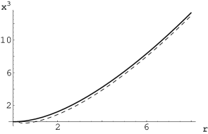
Figure 1: In this figure we represent the function $x^{3}(r)$ for the wall defect in the non-abelian background (solid line). The dashed line represents $x^{3}(r)$ for the abelian background as given by eq. (3.46). In both cases the constant of integration has been fixed by requiring that the minimal value of $x^{3}$ is 0.

4 Two-dimensional defects

In this section we will determine BPS configurations of a D5-brane which extends along two Minkowski coordinates (say $x^{0}$ and $x^{1}$) and along a four-dimensional submanifold embedded in the internal part of the metric (2.1). Such branes would be a two-dimensional object from the gauge theory perspective and, actually, we will find that they preserve the same supersymmetries as a D1-string stretched along $x^{1}$. In order to find these configurations from the kappa symmetry condition $\Gamma_{\kappa}\,\epsilon\,=\,\epsilon$ let us choose the following set of worldvolume coordinates for the D5-brane:

$$\xi^{\mu}\,=\,(x^{0},x^{1},\theta_{1},\phi_{1},\theta_{2},\phi_{2})\,\,,$$ (4.1)

and let us consider an embedding of the type

$$r\,=\,r(\theta_{1},\theta_{2})\,\,,\,\,\,\,\,\,\,\,\,\,\,\,\,\,\,\,\,\psi=\psi(\phi_{1},\phi_{2})\,\,,$$ (4.2)

with $x^{2}$ and $x^{3}$ being constant. From our general expression (2.21) it is straightforward to prove that in this case $\Gamma_{\kappa}\,\epsilon$ is given by:

$$\Gamma_{\kappa}\,\epsilon\,=\,{e^{\phi}\over\sqrt{-g}}\,\,\Gamma_{x^{0}x^{1}}\,\gamma_{\theta_{1}\phi_{1}\theta_{2}\phi_{2}}\,\epsilon\,\,.$$ (4.3)

The induced Dirac matrices $\gamma_{\theta_{i}}$ and $\gamma_{\phi_{i}}$ are easily obtained by using in eq. (2.17) the vielbein coefficients $E_{N}^{\underline{M}}$ and our ansatz. With the purpose of writing these matrices in a convenient form, let us define the quantities:

$$\Delta_{i}\equiv{1\over 2}\,{\cos\theta_{i}\,+\,\partial_{\phi_{i}}\psi\over\sin\theta_{i}}\,\,,$$ (4.4)

in terms of which the $\gamma$-matrices are:

$$e^{-{\phi\over 2}}\,\gamma_{\theta_{1}} = e^{h}\Gamma_{1}\,+\,{a\over 2}\,\hat{\Gamma}_{1}\,+\,\partial_{\theta_{1}}r\,\Gamma_{r}\,\,,$$

$${e^{-{\phi\over 2}}\over\sin\theta_{1}}\,\gamma_{\phi_{1}} = e^{h}\,\Gamma_{2}\,-\,{a\over 2}\,\hat{\Gamma}_{2}\,+\,\Delta_{1}\,\hat{\Gamma}_{3}\,\,,$$

$$e^{-{\phi\over 2}}\,\gamma_{\theta_{2}} = {1\over 2}\cos\psi\,\hat{\Gamma}_{1}\,-\,{1\over 2}\,\sin\psi\,\hat{\Gamma}_{2}\,+\,\partial_{\theta_{2}}r\,\Gamma_{r}\,\,,$$

$${e^{-{\phi\over 2}}\over\sin\theta_{2}}\,\gamma_{\phi_{2}} = {1\over 2}\sin\psi\,\hat{\Gamma}_{1}\,+\,{1\over 2}\cos\psi\,\hat{\Gamma}_{2}\,+\,\Delta_{2}\,\hat{\Gamma}_{3}\,\,.$$ (4.5)

By using eqs. (4.5) and (2.7) the action of the antisymmetrized product of the $\gamma$’s on the Killing spinors $\epsilon$ can be readily obtained. It is of the form:

$${e^{-2\phi}\over\sin\theta_{1}\sin\theta_{2}}\,\,\gamma_{\theta_{1}\phi_{1}\theta_{2}\phi_{2}}\,\epsilon\, = \,\big{[}\,b_{I}\,+\,b_{2\hat{2}}\,\Gamma_{2}\hat{\Gamma}_{2}\,+\,b_{12}\,\Gamma_{12}\,+\,b_{1\hat{2}}\,\Gamma_{1}\hat{\Gamma}_{2}\,+\,b_{1\hat{3}}\,\Gamma_{1}\hat{\Gamma}_{3}\,+\,$$ (4.6)

$$+\,b_{\hat{1}\hat{3}}\,\hat{\Gamma}_{13}\,+\,b_{\hat{2}\hat{3}}\,\hat{\Gamma}_{23}\,+\,b_{2\hat{3}}\,\Gamma_{2}\hat{\Gamma}_{3}\,\big{]}\,\epsilon\,\,,$$

where the $b$’s are functions whose expression depends on the embedding of the probe. In order to write them more compactly let us define $\Lambda_{1}$ and $\Lambda_{2}$ as follows:

$$\Lambda_{1}\equiv{1\over 4}\,\Big{[}\,\partial_{\theta_{1}}r-a\cos\psi\,\partial_{\theta_{2}}r\,\Big{]}\Delta_{1}\,+\,\,\Big{[}(\,e^{2h}-{a^{2}\over 4}\,)\partial_{\theta_{2}}r\,+\,{a\over 4}\cos\psi\,\partial_{\theta_{1}}r\,\Big{]}\,\Delta_{2}\,,$$

$$\Lambda_{2}\equiv-{e^{h}\over 2}\,\Big{[}\,\cos\psi\,\partial_{\theta_{1}}r\,-\,2a\,\partial_{\theta_{2}}r\,\Big{]}\,\Delta_{2}\,+\,{e^{h}\over 2}\,\cos\psi\,\partial_{\theta_{2}}r\,\Delta_{1}\,\,,$$ (4.7)

where $\Delta_{1}$ and $\Delta_{2}$ have been defined in eq. (4.4). Then, the coefficients of the different matrix structures appearing on the right-hand side of eq. (4.6) are:

$$b_{I}\,=\,\Lambda_{1}\cos\alpha\,-\,\Lambda_{2}\sin\alpha\,-\,{e^{2h}\over 4}\,\,\,,$$

$$b_{2\hat{2}}\,=\,\Lambda_{1}\sin\alpha\,+\,\Lambda_{2}\cos\alpha\,\,,$$

$$b_{12}\,=\,-\,{e^{h}\sin\psi\over 2}\,\Big{[}\,\partial_{\theta_{2}}r\,\Delta_{1}\,-\,\,\partial_{\theta_{1}}r\,\Delta_{2}\,\Big{]}\,\sin\alpha\,\,,$$

$$b_{1\hat{2}}\,=\,{e^{h}\sin\psi\over 2}\,\Big{[}\,\,\partial_{\theta_{2}}r\,\Delta_{1}\,-\,\partial_{\theta_{1}}r\,\Delta_{2}\,\Big{]}\,\cos\alpha\,\,,$$

$$b_{1\hat{3}}\,=\,{e^{h}\over 2}\,\sin\psi\Big{[}\,\partial_{\theta_{2}}r\,(\,e^{h}\sin\alpha\,+\,{a\over 2}\cos\alpha\,)\,-\,{a\over 2}\,\Delta_{2}\,\Big{]}\,\,,$$

$$b_{\hat{1}\hat{3}}\,=\,{e^{h}\over 2}\,\sin\psi\Big{[}\,\,\partial_{\theta_{2}}r\,(\,e^{h}\cos\alpha\,-\,{a\over 2}\sin\alpha\,)\,+\,e^{h}\,\Delta_{2}\,\Big{]}\,\,,$$

$$b_{\hat{2}\hat{3}}\,=\,{e^{h}\over 2}\,\cos\psi\Big{[}\,\partial_{\theta_{2}}r\,(\,e^{h}\cos\alpha\,-\,{a\over 2}\sin\alpha\,)\,+\,e^{h}\,\Delta_{2}\,\Big{]}\,+\,{e^{h}\over 4}\,\partial_{\theta_{1}}r\,\sin\alpha\,\,,$$

$$b_{2\hat{3}}\,=\,{e^{h}\over 2}\,\cos\psi\Big{[}\,{a\over 2}\,\Delta_{2}\,-\,\partial_{\theta_{2}}r\,(\,e^{h}\sin\alpha\,+\,{a\over 2}\cos\alpha\,)\,\Big{]}\,+\,{e^{h}\over 4}\,\Big{[}\,\Delta_{1}\,+\,\partial_{\theta_{1}}r\,\cos\alpha\,\Big{]}\,\,.\qquad\qquad$$ (4.8)

By inspecting the right-hand side of eq. (4.6) one immediately realizes that the terms containing the matrix $\hat{\Gamma}_{3}$ give rise to contributions to $\Gamma_{\kappa}$ which do not commute with the projection $\Gamma_{12}\,\epsilon\,=\,\hat{\Gamma}_{12}\,\epsilon$ satisfied by the Killing spinors (see eq. (2.7)). Then, if we want that the supersymmetry preserved by the probe be compatible with that of the background, the coefficients of these terms must vanish. Moreover, we would like to obtain embeddings of the D5-brane probe which preserve the same supersymmetry as a D1-string extended along the $x^{1}$ direction. Accordingly, we shall require the vanishing of all terms on the right-hand side of eq. (4.6) except for the one proportional to the unit matrix, i.e.:

$$b_{2\hat{2}}\,=\,b_{12}\,=\ b_{1\hat{2}}\,=\,b_{1\hat{3}}\,=\,b_{\hat{1}\hat{3}}\,=\,b_{\hat{2}\hat{3}}\,=\,b_{2\hat{3}}\,=\,0\,\,\,.$$ (4.9)

By plugging the explicit form of the $b$’s in (4.9), one gets a system of differential equations for the embedding which will be analyzed in the rest of this section.

4.1 Abelian worldvolume solitons

The above equations (4.9) are quite complicated. In order to simplify the problem, let us consider first the equations for the embedding in the abelian background, which can be obtained from the general ones by putting $a=\alpha=0$. In this case from $b_{\hat{2}\hat{3}}=b_{2\hat{3}}=0$ we get $\,\partial_{\theta_{i}}r=-\Delta_{i}$, where the $\Delta_{i}$’s have been defined in eq. (4.4). More explicitly:

$$\partial_{\theta_{i}}r\,=\,-{1\over 2}\,{\cos\theta_{i}+\partial_{\phi_{i}}\psi\over\sin\theta_{i}}\,\,.$$ (4.10)

One can verify that the other $b^{\prime}s$ in (4.9) vanish if these differential equations are satisfied. Let us see the form of the kappa symmetry condition when the BPS equations (4.10) are satisfied. For the abelian background, the determinant of the induced metric is given by:

$$\sqrt{-g}\,=\,{e^{3\phi}\over 4}\,\,\sin\theta_{1}\,\sin\theta_{2}\,\Big{[}\,(\partial_{\theta_{1}}r)^{2}\,+\,4e^{2h}\,(\partial_{\theta_{2}}r)^{2}\,+\,e^{2h}\,\Big{]}^{{1\over 2}}\,\,\Big{[}\,\Delta_{1}^{2}\,+\,4e^{2h}\,\Delta_{2}^{2}\,+\,e^{2h}\,\Big{]}^{{1\over 2}}\,\,,$$ (4.11)

and the coefficient $b_{I}$ is:

$$b_{I}\,=\,{1\over 4}\,\partial_{\theta_{1}}r\,\Delta_{1}\,+\,e^{2h}\,\partial_{\theta_{2}}r\,\Delta_{2}\,-\,{e^{2h}\over 4}\,\,\,.$$ (4.12)

If the BPS equations $\,\partial_{\theta_{i}}r=-\Delta_{i}$ hold, one can verify by inspection that:

$$e^{-3\phi}\,\sqrt{-g}_{\,|_{BPS}}\,=\,-\sin\theta_{1}\sin\theta_{2}\,b_{I\,|_{BPS}}\,\,,$$ (4.13)

and, thus, the kappa symmetry condition (2.18) becomes

$$\Gamma_{x^{0}x^{1}}\epsilon\,=-\,\epsilon\,\,,$$ (4.14)

which indeed corresponds to a D1 string extended along $x^{1}$. In this abelian case the spinors $\epsilon$ and $\eta$ in eq. (2.10) differ in a function which commutes with everything. Therefore, the condition (4.14) translates into the same condition for the constant spinor $\eta$, namely:

$$\Gamma_{x^{0}x^{1}}\eta\,=-\,\eta\,\,.$$ (4.15)

It follows that this configuration is 1/16 supersymmetric: it preserves the two supersymmetries determined by eqs. (2.11) and (4.15).

4.1.1 Integration of the first-order equations

The BPS equations (4.10) relate the partial derivatives of $r$ with those of $\psi$. According to our ansatz (4.2) the only dependence on $\phi_{1}$ and $\phi_{2}$ in (4.10) comes from the derivatives of $\psi$. Therefore, for consistency of eq. (4.10) with our ansatz we must have:

$$\partial_{\phi_{1}}\psi\,=\,n_{1}\,\,,\,\,\,\,\,\,\,\,\,\,\,\,\,\,\,\,\,\,\,\,\,\,\,\,\partial_{\phi_{2}}\psi\,=\,n_{2}\,\,,$$ (4.16)

where $n_{1}$ and $n_{2}$ are two constant numbers. Thus, $\psi$ must be given by:

$$\psi\,=\,n_{1}\phi_{1}\,+\,n_{2}\phi_{2}\,+\,{\rm constant}\,\,.$$ (4.17)

Using this form of $\psi(\phi_{1},\phi_{2})$ in eq. (4.10) , one can easily integrate $r(\theta_{1},\theta_{2})$, namely:

$$e^{2r}\,=\,{C\over\Big{(}\,\sin{\theta_{1}\over 2}\,\Big{)}^{n_{1}+1}\,\,\Big{(}\,\cos{\theta_{1}\over 2}\,\Big{)}^{1-n_{1}}\,\,\Big{(}\,\sin{\theta_{2}\over 2}\,\Big{)}^{n_{2}+1}\,\,\Big{(}\,\cos{\theta_{2}\over 2}\,\Big{)}^{1-n_{2}}}\,\,,$$ (4.18)

where $C$ is a constant. From the analysis of eq. (4.18) one easily concludes that not all the values of the constants $n_{1}$ and $n_{2}$ are possible. Indeed, the left-hand side of eq. (4.18) is always greater than one, whereas the right-hand side always vanishes for some value of $\theta_{i}$ if $|n_{i}|>1$. Actually, we will verify in the next subsection that only when $n_{1}=n_{2}=0$ (i.e. when $\psi={\rm constant}$) we will be able to generalize the embedding to the non-abelian geometry. Therefore, from now on we will concentrate only in this case, which we rewrite as:

$$e^{2r}\,=\,{e^{2r_{*}}\over\sin\theta_{1}\sin\theta_{2}}\,\,,\qquad\qquad(n_{1}=n_{2}=0)\,\,,$$ (4.19)

where $r_{*}=r(\theta_{1}=\pi/2,\theta_{2}=\pi/2)$ is the minimal value of $r$. It is clear from (4.19) that $r$ diverges at $\theta_{i}=0,\pi$. Therefore our effective strings extend infinitely in the holographic coordinate $r$.

4.2 Non-Abelian worldvolume solitons

Let us consider now the more complicated case of the non-abelian background. We are going to argue that the kappa symmetry condition can only be solved if $\psi$ is constant and $\sin\psi=0$. Indeed, let us assume that $\sin\psi$ does not vanish. If this is the case, by combining the conditions $b_{\hat{1}\hat{3}}=0$ and $b_{\hat{2}\hat{3}}=0$ one gets $\partial_{\theta_{1}}r=0$. Using this result in the equation $b_{12}=0$, one concludes that $\partial_{\theta_{2}}r=0$ (notice that the functions $\Delta_{i}$ can never vanish). However, if $r$ is independent of the $\theta_{i}$’s the equation $b_{1\hat{3}}=0$ can never be fulfilled. Thus, we arrive at a contradiction that can only be resolved if $\sin\psi=0$. Then, one must have:

$$\psi=0,\pi,2\pi,3\pi=0\,\,({\hbox{\rm mod}}\,\pi)\,\,.$$ (4.20)

Let us now define

$$\lambda\equiv\cos\psi=\pm 1\,\,.$$ (4.21)

Thus, in this non-abelian case we are only going to have zero-winding embeddings, i.e., as anticipated above, only the solutions with $n_{1}=n_{2}=0$ in eq. (4.18) generalize to the non-abelian case. Since $\psi$ is constant, we now have

$$\Delta_{i}={1\over 2}\,\cot\theta_{i}\,\,.$$ (4.22)

When $\sin\psi=0$ the equations $b_{12}=b_{1\hat{2}}=b_{\hat{1}\hat{3}}=b_{1\hat{3}}=0$ are automatically satisfied. Moreover, the conditions $b_{\hat{2}\hat{3}}=b_{2\hat{3}}=0$ reduce to:

$$\sin\alpha\,\partial_{\theta_{1}}r\,+\,2\lambda\,\big{(}\,e^{h}\cos\alpha\,-\,{a\over 2}\,\sin\alpha\,\big{)}\,\partial_{\theta_{2}}r\,+\,\lambda e^{h}\,\cot\theta_{2}\,=\,0\,\,,$$

$$\cos\alpha\,\partial_{\theta_{1}}r\,-\,2\lambda\,\big{(}\,e^{h}\sin\alpha\,+\,{a\over 2}\,\cos\alpha\,\big{)}\,\partial_{\theta_{2}}r\,+\,{\lambda a\over 2}\,\cot\theta_{2}\,+\,{1\over 2}\,\cot\theta_{1}\,=\,0\,\,.\qquad$$ (4.23)

From eq. (4.23) one can obtain the values of the partial derivatives of $r$. Indeed, let us define

$$\Delta_{\theta_{1}} \equiv {1\over 2}\,\cot\theta_{1}\coth(2r)\,+\,{\lambda\over 2}\,\,{\cot\theta_{2}\over\sinh(2r)}\,\,,$$

$$\Delta_{\theta_{2}} \equiv {1\over 2}\,\cot\theta_{2}\coth(2r)\,+\,{\lambda\over 2}\,\,{\cot\theta_{1}\over\sinh(2r)}\,\,.$$ (4.24)

Then, one has

$$\partial_{\theta_{i}}r\,=\,-\Delta_{\theta_{i}}\,\,.$$ (4.25)

To derive this result we have used some of the identities written in eq. (3.57). Notice that $\Delta_{\theta_{i}}\rightarrow\Delta_{i}$ when $r\rightarrow\infty$ and the non-abelian BPS equations (4.25) coincide with the abelian ones in eq. (4.10) for $n_{1}=n_{2}=0$ in this limit. After some calculation one can check that $b_{2\hat{2}}$ also vanishes as a consequence of (4.25). Indeed, one can prove that $b_{2\hat{2}}$ can be written:

$$b_{2\hat{2}}\,=\,{\lambda e^{h}\over 2}\,\Big{[}\,\Delta_{\theta_{1}}\,\partial_{\theta_{2}}r\,-\,\Delta_{\theta_{2}}\,\partial_{\theta_{1}}r\,\Big{]}\,\,,$$ (4.26)

which clearly vanishes if eq. (4.25) is satisfied.

For a general function $r(\theta_{1},\theta_{2})$, when the angle $\psi$ takes the values written in eq. (4.20), the determinant of the induced metric takes the form:

$$\sqrt{-g}\,=\,{e^{3\phi}\over 4}\,\sin\theta_{1}\,\sin\theta_{2}\Big{[}(\partial_{\theta_{1}}r)^{2}\,+\,4(e^{2h}\,+\,{a^{2}\over 4}\,)(\partial_{\theta_{2}}r)^{2}\,-\,2a\lambda\partial_{\theta_{1}}r\partial_{\theta_{2}}r\,+\,e^{2h}\,\Big{]}^{{1\over 2}}\times$$

$$\,\,\,\,\,\,\,\,\,\,\,\,\,\,\,\,\,\,\,\,\,\,\,\,\,\,\,\,\,\,\,\,\,\,\,\,\,\,\times\Big{[}\,\Delta_{\theta_{1}}^{2}\,+\,4(e^{2h}\,+\,{a^{2}\over 4}\,)\,\Delta_{\theta_{2}}^{2}\,-\,2a\lambda\Delta_{\theta_{1}}\Delta_{\theta_{2}}\,+\,e^{2h}\,\Big{]}^{{1\over 2}}\,\,.$$ (4.27)

If the BPS equations (4.25) are satisfied, the two factors under the square root on the right-hand side of eq. (4.27) become equal. Moreover, one can prove that:

$$b_{I}\,=\,{1\over 4}\,\partial_{\theta_{1}}r\,(\Delta_{\theta_{1}}-\lambda a\Delta_{\theta_{2}})\,+\,{1\over 4}\,\partial_{\theta_{2}}r\,\Big{(}4\,(e^{2h}\,+\,{a^{2}\over 4}\,)\,\Delta_{\theta_{2}}-\lambda a\Delta_{\theta_{1}}\Big{)}\,-\,{e^{2h}\over 4}\,\,.$$ (4.28)

Using this result one can demonstrate, after some calculation, that eq. (4.13) is also satisfied in this non-abelian case. As a consequence, the kappa symmetry projection reduces to the one written in eq. (4.14), i.e. to that corresponding to a D1-brane.

4.2.1 Integration of the first-order equations

In order to integrate the first order equations (4.25) for $r(\theta_{1},\theta_{2})$, let us define the new variable $y(r)$ as:

$$y(r)\equiv\cosh(2r)\,\,.$$ (4.29)

In terms of $y$, the BPS system (4.25) can be greatly simplified, namely:

$$\partial_{\theta_{1}}y\,+\,\cot\theta_{1}\,y = -\lambda\cot\theta_{2}\,\,,$$

$$\partial_{\theta_{2}}y\,+\,\cot\theta_{2}\,y = -\lambda\cot\theta_{1}\,\,,$$ (4.30)

which can be easily integrated by the method of variation of constants. In terms of the original variable $r$ one has:

$$\cosh(2r)\,=\,{\cosh(2r_{*})\,+\,\lambda\cos\theta_{1}\cos\theta_{2}\over\sin\theta_{1}\sin\theta_{2}}\,\,,$$ (4.31)

where $r_{*}\equiv r(\theta_{1}=\pi/2,\theta_{2}=\pi/2)$ is the minimal value of $r$. This is a remarkably simple solution for the very complicated system of kappa symmetry equations. Notice that there are two solutions for $r(\theta_{1},\theta_{2})$, which correspond to the two possible values of $\lambda$ on the right-hand side of (4.31). If $\lambda=+1$ ($\lambda=-1$) the angle $\psi$ is fixed to $\psi=0,2\pi$ ($\psi=\pi,3\pi$). Thus, the $U(1)$ symmetry $\psi\rightarrow\psi+\epsilon$ of the abelian case is broken to ${\rm Z}\kern-3.8pt{\rm Z}\kern 2.0pt_{2}$, reflecting the same breaking that occurs in the geometry. Moreover, it follows from (4.31) that $r$ diverges at $\theta_{1,2}=0,\pi$. It is easily proved that the embedding written in eqs. (4.20) and (4.31) satisfies the equations of motion of the probe and, actually, it saturates a BPS energy bound (see appendix A). Moreover, in appendix B we will find new codimension two defects in the non-abelian background for which the angle $\psi$ is not constant.

5 Concluding remarks

In this paper we have systematically studied the possibility of adding supersymmetric configurations of D5-brane probes in the MN background in such a way that they create a codimension one or two defect in the gauge theory directions. The technique, thoroughly explained in sections 2 and 3, consists of using kappa symmetry to look for a system of first-order equations which guarantee that the supersymmetry preserved by the worldvolume of the probe is consistent with that of the background. Although the general system of equations obtained from kappa symmetry is very involved, the solutions we have found are remarkably simple. For a given election of worldvolume coordinates and a given ansatz for the embedding, chosen for their simplicity and physical significance, the result is unique.

In order to extract consequences of our results in the gauge theory dual, some additional work must be done. First of all, one can study the fluctuations of the probes around the configurations found here and one can try to obtain the dictionary between these fluctuations and the corresponding operators in the field theory side, along the lines of refs. [5, 9]. In the analysis of these fluctuations we will presumably find the difficulties associated with the UV blowup of the dilaton, which could be overcome by using the methods employed in ref. [19] in the case of flavor branes (see also ref. [25] for a similar approach in the case of the glueball spectrum of the MN background). Once this fluctuation-operator dictionary is obtained we could try to give some meaning to the functions $x^{3}(r)$ and $r(\theta_{1},\theta_{2})$ of eqs. (3.68) and (4.31) respectively, which should encode some renormalization group flow of the defect theory.

Let us also point out that one could explore with the same techniques employed here some other supergravity backgrounds (such as the one obtained in [26], which are dual to ${\cal N}=1$, $d=3$ super Yang-Mills theory) and try to find the configurations of probes which introduce supersymmetric defects in the field theory. It is also worth mentioning that, although we have focussed here on the analysis of the supersymmetric objects in the MN background, we could have stable non-supersymmetric configurations, such as the confining strings of ref. [27], which are constructed from D3-branes wrapping a two-sphere. Another example of an interesting non-supersymmetric configuration is the baryon vertex, which consists of a D3-brane wrapped on a three-cycle which captures the RR flux [28].

Finally, it is also interesting to figure out which kind of brane configurations of the type IIA theory correspond to the different objects studied throughout this paper and, moreover, how they would uplift to M-theory, working along the lines of [29].

The MN construction of ${\cal N}=1$ Yang-Mills in the type IIB theory by wrapping D5-branes in a finite holomorphic two-cycle of a $CY_{3}$ corresponds in the type IIA theory to D6 branes wrapping a SLag three cycle inside a $CY_{3}$, which, when going to eleven dimensions, gets uplifted to a $G_{2}$ holonomy manifold. We have seen that codimension one objects preserving two supercharges can be added by including D5-branes wrapping a supersymmetric three-cycle. In the type IIA theory, supersymmetric codimension one objects can be introduced by adding a D4-brane wrapping a holomorphic two-cycle (this is how domain walls are introduced in ${\cal N}=1$ four dimensional field theories, see, for instance [30]) or by considering a D6-brane wrapping a divisor four-cycle of the $CY_{3}$. This first configuration uplifts to a M5 wrapping an associative three cycle inside the $G_{2}$ manifold, whereas the second yields a cohomogeneity two $Spin(7)$ holonomy manifold. The two cohomogeneous directions are the one corresponding to the energy scale and the distance to the defect. The codimension two objects, introduced by wrapping a D5-brane in a four-cycle yield D4-branes wrapping a susy SLag three-cycle in the type IIA theory, which therefore uplift to a configuration where M5-branes wrap the coassociative four-cycle of the $G_{2}$ manifold. Finally, notice that, if both kind of codimension one and two objects are parallel, they can be added simultaneously, preserving just one supercharge. The corresponding M-theory setup could consist of a stack of M5-branes wrapping a Cayley four-cycle inside the $Spin(7)$ manifold described above. In this case, both the codimension one and two objects are extended along the flat directions transverse to the $Spin(7)$ manifold.

Appendix A Energy bounds

The lagrangian density for a D5-brane probe in the Maldacena-Nuñez background is given by:

$${\cal L}\,=\,-e^{-\phi}\,\sqrt{-g}\,-\,P[\,C^{(6)}\,]\,\,,$$ (A.1)

where we have taken the string tension equal to one and $P[\,C^{(6)}\,]$ denotes the pullback of the RR potential written in eqs. (2.13) and (2.14). In eq. (A.1) we have already taken into account that we are considering configurations of the probe with vanishing worldvolume gauge field. For static embeddings, such as the ones obtained in the main text, the hamiltonian density ${\cal H}$ is just ${\cal H}=-{\cal L}$. In this appendix we are going to verify that, for the systems studied in sections 3 and 4, ${\cal H}$ satisfies a lower bound, which is saturated just when the corresponding BPS equations are satisfied. Actually, we will verify that, for a generic embedding, ${\cal H}$ can be written as:

$${\cal H}\,=\,{\cal Z}\,+\,{\cal S}\,\,,$$ (A.2)

where ${\cal Z}$ is a total derivative and ${\cal S}$ is non-negative:

$${\cal S}\,\geq\,0\,\,.$$ (A.3)

From eqs. (A.2) and (A.3) it follows immediately that ${\cal H}\geq{\cal Z}$, which is the energy bound we are looking for. Moreover, we will check that ${\cal S}=0$ precisely when the BPS equations obtained from kappa symmetry are satisfied, which means that the energy bound is saturated for these configurations. These facts mean that the configurations we have found are not just solutions of the equations of motion but BPS worldvolume solitons of the D5-brane probe [31].

A.1 Energy bound for the wall solutions

Let us consider a D5-brane probe in the non-abelian Maldacena-Nuñez background and let us choose the same worldvolume coordinates as in eq. (3.1) and the ansatz (3.2) for the embedding. For simplicity we will consider the angular embeddings $\theta_{2}(\theta_{1},\phi_{1})$ and $\phi_{2}(\theta_{1},\phi_{1})$ written in eq. (3.45) and we will consider a completely arbitrary function $x^{3}(r)$. Using the value of $\sqrt{-g}$ given in (3.63), one gets:

$${\cal H}\,=\,-{\cal L}\,=\,e^{2\phi}\,\sin\theta_{1}\,\Bigg{[}\,{r\over\sinh 2r}\,\big{(}\,\cosh 2r\,-\,\lambda m\,\big{)}\,\sqrt{1\,+\,(\partial_{r}x^{3})^{2}}\,-\,{\lambda m\over 4}\,a^{\prime}\,\partial_{r}x^{3}\,\Bigg{]}\,\,,\qquad$$ (A.4)

where $m=\pm 1$ is the same as in eq. (3.45) and $\lambda=\cos\psi_{0}\,=\,\pm 1$ (see eq. (3.61)). In order to write ${\cal H}$ as in eq. (A.2) , let us define the function

$$\Lambda_{r}\equiv e^{-h}\,\bigg{[}\,r\coth 2r\,-\,{1\over 2}\,\bigg{]}\,\,.$$ (A.5)

Notice that the BPS equation for $x^{3}(r)$ (eq. (3.68)) is just $\partial_{r}x^{3}=\Lambda_{r}$. Furthermore, $a^{\prime}$ can be written in terms of $\Lambda_{r}$ as:

$${a^{\prime}\over 4}\,=\,-{e^{h}\Lambda_{r}\over\sinh 2r}\,\,.$$ (A.6)

Using this last result, we can write ${\cal H}$ as :

$${\cal H}\,=\,\sin\theta_{1}\,{e^{2\phi}\over\sinh 2r}\,\Bigg{[}\,r\,\big{(}\,\cosh 2r\,-\,\lambda m\,\big{)}\,\sqrt{1\,+\,(\partial_{r}x^{3})^{2}}\,+\,\lambda me^{h}\,\Lambda_{r}\,\partial_{r}x^{3}\,\Bigg{]}\,\,.$$ (A.7)

Let us now write ${\cal H}$ as in eq. (A.2), with:

$${\cal Z}\,=\,\sin\theta_{1}\,{e^{2\phi+h}\over\sinh 2r}\,\Bigg{[}\,\cosh 2r\,\Lambda_{r}\,\partial_{r}x^{3}\,+\,\cosh 2r\,-\,\lambda m\,\Bigg{]}\,\,.$$ (A.8)

By using eq. (3.64), one can prove that

$${\cal H}_{\,\,|BPS}\,=\,{\cal Z}_{\,\,|BPS}\,\,.$$ (A.9)

Moreover, ${\cal Z}$ can be written as a total derivative, i.e. ${\cal Z}\,=\,\partial_{r}{\cal Z}^{r}\,+\,\partial_{\theta_{1}}{\cal Z}^{\theta_{1}}$, with

$${\cal Z}^{r}\,=\,\sin\theta_{1}\,{e^{2\phi+h}\over\sinh 2r}\,\Bigg{[}\,\cosh 2r\,\Lambda_{r}\,x^{3}\,+\,{\sinh 2r\over 2}\,-\,\lambda mr\,\Bigg{]}\,\,,$$

$${\cal Z}^{\theta_{1}}\,=\,\cos\theta_{1}\,e^{2\phi}\,\Bigg{[}\,2e^{2h}\,+\,{1-a^{4}\over 8}\,e^{-2h}\,\Bigg{]}\,x^{3}\,\,.$$ (A.10)

To derive this result it is useful to remember that $e^{2\phi+h}/\sinh 2r$ is constant and use the relation

$$\partial_{r}\,\bigg{[}\,\cosh 2r\Lambda_{r}\,\bigg{]}\,=\,e^{-h}\,\sinh 2r\,\bigg{[}\,2e^{2h}\,+\,{1-a^{4}\over 8}\,e^{-2h}\,\bigg{]}\,\,,$$ (A.11)

which can be proved by direct calculation. Moreover, taking into account that $r=e^{h}\,\sqrt{1+\Lambda_{r}^{2}}$ (see eq. (3.64)), one can write ${\cal S}$ as:

$${\cal S}\,=\,\sin\theta_{1}\,{e^{2\phi+h}\over\sinh 2r}\,\big{(}\,\cosh 2r\,-\,\lambda m\,\big{)}\,\Bigg{[}\,\sqrt{1+\Lambda_{r}^{2}}\,\sqrt{1\,+\,(\partial_{r}x^{3})^{2}}\,-\,(\,1\,+\,\Lambda_{r}\partial_{r}x^{3}\,)\,\Bigg{]}\,\,,$$ (A.12)

and it is straightforward to verify that ${\cal S}\geq 0$ is equivalent to

$$(\,\partial_{r}x^{3}\,-\,\Lambda_{r}\,)^{2}\geq 0\,\,,$$ (A.13)

which is obviously always satisfied for any function $x^{3}(r)$ and reduces to an equality when the BPS equation (3.68) holds.

A.2 Energy bound for the effective string solutions

We will now consider the configurations studied in section 4. Accordingly, let us choose worldvolume coordinates as in (4.1) and an embedding of the type displayed in eq. (4.2) in the non-abelian MN background, where, for simplicity, we will take the angle $\psi$ to be a constant such that $\sin\psi=0$ (see eq. (4.20)). In this case it is also easy to prove that the hamiltonian density can be written as in eq. (A.2), where for an arbitrary function $r(\theta_{1},\theta_{2})$, ${\cal Z}$ is a total derivative and ${\cal S}\geq 0$. In order to verify these facts, let us take ${\cal Z}$ to be:

$${\cal Z}\,=\,{e^{2\phi}\over 4}\,\sin\theta_{1}\,\sin\theta_{2}\,\Big{[}\,e^{2h}-(\Delta_{\theta_{1}}-\lambda a\Delta_{\theta_{2}})\partial_{\theta_{1}}r\,-\,\Big{(}4\,(e^{2h}\,+\,{a^{2}\over 4}\,)\,\Delta_{\theta_{2}}-\lambda a\Delta_{\theta_{1}}\Big{)}\partial_{\theta_{2}}r\,\Big{]}\,\,.\qquad$$

(A.14)

One can prove that ${\cal Z}$ is a total derivative. Indeed, let us introduce the functions $z_{1}(r)$ and $z_{2}(r)$ as the solutions of the equations:

$${dz_{1}\over dr}\,=\,\cos\alpha\,{e^{2\phi}\over 8}\,\,,$$

$${dz_{2}\over dr}\,=\,-\,\Big{[}\,a\cos\alpha\,+\,2e^{h}\sin\alpha\,\Big{]}\,{e^{2\phi}\over 8}\,\,,$$ (A.15)

where $h$, $\phi$ and $\alpha$, are the functions of the radial coordinate displayed in eqs. (2.4) and (2.9). Then, one can verify that ${\cal Z}\,=\,\partial_{\theta_{1}}\,{\cal Z}^{\theta_{1}}\,+\,\partial_{\theta_{2}}\,{\cal Z}^{\theta_{2}}$, where

$${\cal Z}^{\theta_{1}} = -\cos\theta_{1}\sin\theta_{2}\,z_{1}\,+\,\lambda\sin\theta_{1}\cos\theta_{2}\,z_{2}\,\,,$$

$${\cal Z}^{\theta_{2}} = -\sin\theta_{1}\cos\theta_{2}\Big{[}\,{e^{2\phi+2h}\over 4}\,-\,z_{1}\,\Big{]}\,-\,\lambda\cos\theta_{1}\sin\theta_{2}\,z_{2}\,\,.$$ (A.16)

In order to prove this result the following relation:

$${d\over dr}\,\Big{[}\,e^{2\phi+2h}\,\Big{]}\,=\,2re^{2\phi}\,\,,$$ (A.17)

is quite useful.

It is straightforward to prove that for these configurations the pullback of $C^{(6)}$ vanishes. Therefore (see eq. (A.1)), the hamiltonian density in this case is just ${\cal H}=e^{-\phi}\,\sqrt{-g}$, with $\sqrt{-g}$ given in eq. (4.27). Once ${\cal Z}$ is known and given by the expression written in eq. (A.14), ${\cal S}$ is defined as ${\cal H}-{\cal Z}$. One can verify that ${\cal S}\geq 0$ is equivalent to the condition

$$\Big{[}\,\partial_{\theta_{1}}r+\Delta_{\theta_{1}}\,-\,\lambda a(\partial_{\theta_{2}}r+\Delta_{\theta_{2}})\,\Big{]}^{2}\,+\,4e^{2h}\,\Big{[}\,\partial_{\theta_{2}}r+\Delta_{\theta_{2}}\,\Big{]}^{2}\,+\,4\Big{[}\,\Delta_{\theta_{2}}\partial_{\theta_{1}}r-\Delta_{\theta_{1}}\partial_{\theta_{2}}r\,\Big{]}^{2}\,\geq 0\,\,,$$

which is obviously satisfied and reduces to an identity when the BPS equations (4.25) hold. It is easy to compute the central charge ${\cal Z}$ for the BPS configurations. The result is:

$${\cal Z}_{\,|_{BPS}}\,=\,{e^{2\phi}\over 4}\,\sin\theta_{1}\,\sin\theta_{2}\,\Big{[}\,(\Delta_{\theta_{1}}-\lambda a\Delta_{\theta_{2}})^{2}\,+\,4e^{2h}\,\Delta_{\theta_{2}}^{2}\,+\,e^{2h}\,\Big{]}\,\,.$$ (A.19)

It follows from the above expression that ${\cal Z}_{\,|_{BPS}}$ is always non-negative.

Appendix B More defects

B.1 Wall defects

Let us find more supersymmetric configurations of the D5-brane probe which behave as a codimension one defect from the gauge theory point of view. In particular, we are interested in trying to obtain embeddings for which the angle $\psi$ is not constant. To insure this fact we will include $\psi$ in our set of worldvolume coordinates. Actually, we will choose the $\xi$’s as:

$$\xi^{\mu}\,=\,(x^{0},x^{1},x^{2},\theta_{2},\phi_{2},\psi)\,\,,$$ (B.1)

and we will adopt the following ansatz for the embedding:

$$\theta_{1}=\theta_{1}(\theta_{2}),\,\,\,\,\,\,\,\,\,\,\,\,\,\,\,\phi_{1}=\phi_{1}(\phi_{2}),\,\,$$

$$x^{3}=x^{3}(\psi)\,\,,\,\,\,\,\,\,\,\,\,\,\,\,\,r\,=\,r(\psi)\,\,.$$ (B.2)

For these configurations the kappa symmetry matrix acts on the Killing spinors $\epsilon$ as:

$$\Gamma_{\kappa}\,\epsilon\,=\,{1\over\sqrt{-g}}\,\gamma_{x^{0}x^{1}x^{2}\theta_{2}\phi_{2}\psi}\,\epsilon\,\,.$$ (B.3)

Now the induced gamma matrices are:

$$e^{-{\phi\over 2}}\,\gamma_{x^{\mu}}\,=\,\Gamma_{x^{\mu}}\,\,,\,\,\,\,\,\,\,\,\,\,\,\,\,\,\,\,\,\,(\mu=0,1,2),\,\,$$

$$e^{-{\phi\over 2}}\,\gamma_{\theta_{2}}\,=\,e^{h}\,\partial_{\theta_{2}}\theta_{1}\,\Gamma_{1}\,+\,W_{1\theta}\,\hat{\Gamma}_{1}\,+\,W_{2\theta}\,\hat{\Gamma}_{2}\,\,,$$

$$e^{-{\phi\over 2}}\,\gamma_{\phi_{2}}\,=\,e^{h}\,\sin\theta_{1}\partial_{\phi_{2}}\phi_{1}\,\Gamma_{2}\,+\,W_{1\phi}\,\hat{\Gamma}_{1}\,+\,W_{2\phi}\,\hat{\Gamma}_{2}\,+\,W_{3\phi}\,\hat{\Gamma}_{3}\,\,,$$

$$e^{-{\phi\over 2}}\,\gamma_{\psi}\,=\,{1\over 2}\,\hat{\Gamma}_{3}\,+\,\partial_{\psi}\,r\,\Gamma_{r}\,+\,\partial_{\psi}\,x^{3}\,\Gamma_{x^{3}}\,\,,$$ (B.4)

where the $W$’s are the following quantities:

$$W_{1\theta}\,=\,{1\over 2}\,[\cos\psi\,+\,a\partial_{\theta_{2}}\theta_{1}\,]\,\,,$$

$$W_{2\theta}\,=\,-{1\over 2}\,\sin\psi\,\,,$$

$$W_{1\phi}\,=\,{1\over 2}\,\sin\theta_{2}\sin\psi\,\,,$$

$$W_{2\phi}\,=\,{1\over 2}\,[\,\sin\theta_{2}\cos\psi\,-\,a\sin\theta_{1}\partial_{\phi_{2}}\phi_{1}\,]\,\,,$$

$$W_{3\phi}\,=\,{1\over 2}\,[\cos\theta_{2}\,+\,\partial_{\phi_{2}}\phi_{1}\cos\theta_{1}\,]\,\,.$$ (B.5)

B.1.1 Embeddings at $r=0$

Let us analyze first the possibility of taking in our previous equations $r=0$ and an arbitrary constant value of $x^{3}$. Since $e^{h}\rightarrow 0$, $a\rightarrow 1$ and $\phi\rightarrow\phi_{0}$ when $r\rightarrow 0$, one has in this case $\gamma_{\theta_{2}}=e^{{\phi_{0}\over 2}}[W_{1\theta}\,\hat{\Gamma}_{1}\,+\,W_{2\theta}\,\hat{\Gamma}_{2}]$, $\gamma_{\phi_{2}}=e^{{\phi_{0}\over 2}}[W_{1\phi}\,\hat{\Gamma}_{1}\,+\,W_{2\phi}\,\hat{\Gamma}_{2}\,+\,W_{3\phi}\,\hat{\Gamma}_{3}]$ and $\gamma_{\psi}=e^{{\phi_{0}\over 2}}\hat{\Gamma}_{3}/2$ and one immediately gets:

$$\gamma_{\theta_{2}\phi_{2}\psi}\,\epsilon={e^{{3\over 2}\phi_{0}}\over 8}\,\Big{[}\sin\theta_{2}+(\sin\theta_{2}\,\partial_{\theta_{2}}\theta_{1}-\sin\theta_{1}\partial_{\phi_{2}}\phi_{1})\cos\psi-\sin\theta_{1}\,\partial_{\theta_{2}}\theta_{1}\,\partial_{\phi_{2}}\phi_{1})\,\Big{]}\hat{\Gamma}_{123}\,\epsilon\,\,.\qquad$$ (B.6)

On the other hand, it is easy to compute the value of the determinant of the induced metric for an embedding of the type (B.2) at $r=0$ and constant $x^{3}$. By using this result one readily gets the action of $\Gamma_{\kappa}$ on $\epsilon$. Indeed, let us define $s(\theta_{2},\phi_{2},\psi)$ to be the following sign:

$$s(\theta_{2},\phi_{2},\psi)\equiv{\rm sign}\,\Big{[}\sin\theta_{2}+(\sin\theta_{2}\,\partial_{\theta_{2}}\theta_{1}-\sin\theta_{1}\partial_{\phi_{2}}\phi_{1})\cos\psi-\sin\theta_{1}\,\partial_{\theta_{2}}\theta_{1}\,\partial_{\phi_{2}}\phi_{1})\,\Big{]}\,\,.$$ (B.7)

Then, one has:

$$\Gamma_{\kappa}\epsilon_{\,\,|_{r=0}}\,=\,s\,\Gamma_{x^{0}x^{1}x^{2}}\hat{\Gamma}_{123}\epsilon_{\,\,|_{r=0}}\,\,.$$ (B.8)

It follows that the condition $\Gamma_{\kappa}\epsilon=\epsilon$ is equivalent to the projection:

$$\Gamma_{x^{0}x^{1}x^{2}}\hat{\Gamma}_{123}\epsilon_{\,\,|_{r=0}}\,=\,s\,\epsilon_{\,\,|_{r=0}}\,\,.$$ (B.9)

Notice that the right-hand side of (B.9) only depends on the angular part of the embedding through the sign $s$. Let us rewrite eq. (B.9) in terms of the spinor $\epsilon_{0}$ defined in eq. (3.47). First of all, let us introduce the matrix $\hat{\Gamma}_{*}$ as:

$$\hat{\Gamma}_{*}\,=\,\Gamma_{x^{0}x^{1}x^{2}}\Gamma_{1}\hat{\Gamma}_{23}\,\,.$$ (B.10)

Recall from (3.47) that $\epsilon\,=\,e^{{\alpha\over 2}\,\Gamma_{1}\hat{\Gamma}_{1}}\,\,\epsilon_{0}$. As $\alpha(r=0)=-\pi/2$, see eqs. (2.8) and (2.9), the above condition reduces to:

$$\hat{\Gamma}_{*}\,\epsilon_{0}\,=\,s\,\epsilon_{0}\,\,.$$ (B.11)

It is easy to verify that this condition commutes with the projections satisfied by $\epsilon_{0}$, which are the same as those satisfied by the constant spinor $\eta$ (see eq. (2.11)). Moreover, it is readily checked that these configurations satisfy the equations of motion of the probe. Notice that the angular embedding is undetermined. However, the above projection only makes sense if $s(\theta_{2},\phi_{2},\psi)$ does not depend on the angles. Although the angular embedding is not uniquely determined, there are some embeddings that can be discarded. For example if we take $\theta_{1}=\theta_{2}$, $\phi_{1}=\phi_{2}$ the corresponding three-cycle has vanishing volume and $s$ is not well-defined. For $\theta_{1}=$ constant, $\phi_{1}=$ constant one has $s=1$. The same value of $s$ is obtained if $\theta_{1}=\pi-\theta_{2}$, $\phi_{1}=\phi_{2}$ or when $\theta_{1}=\theta_{2}$, $\phi_{1}=2\pi-\phi_{2}$. Notice that this configuration consists of a D5-brane, which is finite in the internal directions, wrapping the finite $S^{3}$ inside the geometry, which has minimal volume at $r=0$. This object is thought to correspond to a domain wall of the field theory [16, 32]. However, the physics of domain walls is yet not fully understood in this model.

B.1.2 General case

Let us now come back to the general case. By using the relation between the spinors $\epsilon$ and $\epsilon_{0}$, the kappa symmetry equation $\Gamma_{\kappa}\,\epsilon\,=\,\epsilon$ can be rephrased as the following condition on the spinor $\epsilon_{0}$:

$$e^{-{\alpha\over 2}\,\Gamma_{1}\hat{\Gamma}_{1}}\Gamma_{\kappa}e^{{\alpha\over 2}\,\Gamma_{1}\hat{\Gamma}_{1}}\,\,\epsilon_{0}\,=\,\epsilon_{0}\,\,.$$ (B.12)

Let us evaluate the left-hand side of this equation by imposing the projection (B.11), i.e. the same projection as the one satisfied by the supersymmetric configurations at $r=0$. After some calculation one gets an expression of the type:

$$e^{-{\alpha\over 2}\,\Gamma_{1}\hat{\Gamma}_{1}}\Gamma_{\kappa}e^{{\alpha\over 2}\,\Gamma_{1}\hat{\Gamma}_{1}}\,\,\epsilon_{0}\,=\,{e^{3\phi}\over\sqrt{-g}}\,\,\Big{[}\,d_{I}\,+\,d_{1\hat{1}}\,\Gamma_{1}\hat{\Gamma}_{1}\,+\,d_{\hat{1}\hat{2}}\,\hat{\Gamma}_{1}\hat{\Gamma}_{2}\,+\,d_{1\hat{2}}\,\Gamma_{1}\hat{\Gamma}_{2}\,+$$

$$\qquad\qquad\qquad\qquad+d_{\hat{2}\hat{3}}\,\hat{\Gamma}_{2}\hat{\Gamma}_{3}\,+\,d_{2\hat{3}}\,\Gamma_{2}\hat{\Gamma}_{3}\,+\,d_{\hat{1}\hat{3}}\,\hat{\Gamma}_{1}\hat{\Gamma}_{3}\,+\,d_{1\hat{3}}\,\Gamma_{1}\hat{\Gamma}_{3}\,\Big{]}\,\epsilon_{0}\,\,,$$ (B.13)

where the $d$’s depend on the embedding (see below). Clearly, in order to satisfy eq. (B.12) we must require the conditions:

$$d_{1\hat{1}}\,=\,d_{\hat{1}\hat{2}}\,=\,d_{1\hat{2}}\,=\,d_{\hat{2}\hat{3}}\,=\,d_{2\hat{3}}\,=\,d_{\hat{1}\hat{3}}\,=\,d_{1\hat{3}}\,=\,0\,\,.$$ (B.14)

The expressions of the $d$’s are quite involved. In order to write them in a compact form let us define the quantities ${\cal P}_{1}$, ${\cal P}_{2}$ and ${\cal P}_{3}$ as:

$${\cal P}_{1}\,\equiv\,W_{1\theta}\,W_{2\phi}\,-\,W_{1\phi}\,W_{2\theta}\,+\,e^{2h}\,\sin\theta_{1}\,\partial_{\theta_{2}}\theta_{1}\,\partial_{\phi_{2}}\phi_{1}\,\,,$$

$${\cal P}_{2}\,\equiv\,e^{h}\,\Big{(}\,W_{2\phi}\,\partial_{\theta_{2}}\theta_{1}\,-\,W_{1\theta}\,\sin\theta_{1}\,\partial_{\phi_{2}}\phi_{1}\,\Big{)}\,\,,$$

$${\cal P}_{3}\,\equiv\,e^{h}\,\Big{(}\,W_{1\phi}\,\partial_{\theta_{2}}\theta_{1}\,+\,W_{2\theta}\,\sin\theta_{1}\,\partial_{\phi_{2}}\phi_{1}\,\Big{)}\,\,.$$ (B.15)

Then the coefficients of the terms that do not contain the matrix $\hat{\Gamma}_{3}$ are:

$$d_{I}\,=\,{s\over 2}\,\,\Big{[}\,{\cal P}_{2}\cos\alpha\,-\,{\cal P}_{1}\sin\alpha\,\Big{]}\,+\,\Big{[}\,{\cal P}_{1}\cos\alpha\,+\,{\cal P}_{2}\sin\alpha\,\Big{]}\,\partial_{\psi}x^{3}\,+\,s\,{\cal P}_{3}\,\partial_{\psi}r\,,$$

$$d_{1\hat{1}}\,=\,-{s\over 2}\,\,\Big{[}\,{\cal P}_{1}\cos\alpha\,+\,{\cal P}_{2}\sin\alpha\,\Big{]}\,+\,\Big{[}\,{\cal P}_{2}\cos\alpha\,-\,{\cal P}_{1}\sin\alpha\,\Big{]}\,\partial_{\psi}x^{3}\,,$$

$$d_{\hat{1}\hat{2}}\,=\,{s\over 2}\,{\cal P}_{3}\,-\,s\Big{[}\,{\cal P}_{2}\cos\alpha\,-\,{\cal P}_{1}\sin\alpha\,\Big{]}\,\partial_{\psi}r\,,$$

$$d_{1\hat{2}}\,=\,s\,\Big{[}\,{\cal P}_{1}\cos\alpha\,+\,{\cal P}_{2}\sin\alpha\,\Big{]}\,\partial_{\psi}r\,-\,{\cal P}_{3}\,\partial_{\psi}x^{3}\,\,.$$ (B.16)

From the conditions $d_{1\hat{1}}\,=\,d_{\hat{1}\hat{2}}\,=\,0$ we get the BPS equations that determine $\partial_{\psi}x^{3}$ and $\partial_{\psi}r$, namely:

$$\partial_{\psi}x^{3}\,=\,{s\over 2}\,{{\cal P}_{1}\cos\alpha\,+\,{\cal P}_{2}\sin\alpha\over{\cal P}_{2}\cos\alpha\,-\,{\cal P}_{1}\sin\alpha}\,\,,\qquad\qquad\partial_{\psi}r\,=\,{1\over 2}\,{{\cal P}_{3}\over{\cal P}_{2}\cos\alpha\,-\,{\cal P}_{1}\sin\alpha}\,,\,\,.$$ (B.17)

while the equation $d_{1\hat{2}}=0$ is satisfied if the differential equations (B.17) hold.

The expressions of the coefficients of the terms with the matrix $\hat{\Gamma}_{3}$ are:

$$d_{\hat{2}\hat{3}} = -W_{3\phi}\,\Big{[}\,W_{1\theta}\cos\alpha\,+\,e^{h}\,\partial_{\theta_{2}}\theta_{1}\sin\alpha\,\Big{]}\,\partial_{\psi}x^{3}\,\,,$$

$$d_{2\hat{3}} = W_{3\phi}\,\Big{[}\,\Big{(}\,W_{1\theta}\,\sin\alpha\,-\,e^{h}\,\partial_{\theta_{2}}\theta_{1}\cos\alpha\,\Big{)}\partial_{\psi}x^{3}\,-\,s\,W_{2\theta}\,\partial_{\psi}r\,\Big{]}\,\,,$$

$$d_{\hat{1}\hat{3}} = W_{3\phi}\,\Big{[}\,W_{2\theta}\,\partial_{\psi}x^{3}\,-\,s\Big{(}\,e^{h}\,\partial_{\theta_{2}}\theta_{1}\cos\alpha\,-\,W_{1\theta}\,\sin\alpha\,\Big{)}\,\partial_{\psi}r\,\Big{]}\,\,,$$

$$d_{1\hat{3}} = sW_{3\phi}\,\Big{[}\,W_{1\theta}\cos\alpha\,+\,e^{h}\,\partial_{\theta_{2}}\theta_{1}\sin\alpha\,\Big{]}\,\partial_{\psi}r\,\,.$$ (B.18)

Let us impose now the vanishing of the coefficients (B.18). Clearly, this condition can be achieved by requiring that $r$ and $x^{3}$ be constant. It is easy to see from the vanishing of the right-hand side of eq. (B.17) that this only happens at $r=0$ and, therefore, the configuration reduces to the one studied above. Another possibility is to impose $W_{3\phi}=0$, which is equivalent to the following differential equation:

$$-{\cos\theta_{2}\over\cos\theta_{1}}\,=\,\partial_{\phi_{2}}\phi_{1}\,\,.$$ (B.19)

For consistency, both sides of the equation must be equal to a constant which we will denote by $m$:

$$\partial_{\phi_{2}}\phi_{1}\,=\,m\,\,,\qquad\qquad\qquad\cos\theta_{1}\,=\,-{\cos\theta_{2}\over m}\,\,.$$ (B.20)

Moreover, by differentiating the above relation between $\theta_{1}$ and $\theta_{2}$, we immediately obtain:

$$\partial_{\theta_{2}}\theta_{1}\,=\,-{\sin\theta_{2}\over m\sin\theta_{1}}\,=\,-{\rm sign}(m)\,{\sin\theta_{2}\over\sqrt{\sin^{2}\theta_{2}\,+\,m^{2}-1}}\,\,.$$ (B.21)

Moreover, by using eqs. (B.20) and (B.21) one can easily find the following expression of the ${\cal P}$’s:

$${{\cal P}_{1}\over\sin\theta_{2}} = {1\over 4}\,\Big{[}\,1\,+\,a\,\Big{(}\,\partial_{\theta_{2}}\theta_{1}\,+\,{1\over\partial_{\theta_{2}}\theta_{1}}\,\Big{)}\,\cos\psi\,+\,a^{2}\,\Big{]}\,-\,e^{2h}\,\,,$$

$$e^{-h}\,{{\cal P}_{2}\over\sin\theta_{2}} = {1\over 2}\,\Big{(}\,\partial_{\theta_{2}}\theta_{1}\,+\,{1\over\partial_{\theta_{2}}\theta_{1}}\,\Big{)}\,\cos\psi\,+\,a\,\,,$$

$$e^{-h}\,{{\cal P}_{3}\over\sin\theta_{2}} = {1\over 2}\,\Big{(}\,\partial_{\theta_{2}}\theta_{1}\,+\,{1\over\partial_{\theta_{2}}\theta_{1}}\,\Big{)}\,\sin\psi\,\,.$$ (B.22)

For consistency with our ansatz, the right-hand side of the equation for $\partial_{\psi}r$ in (B.17) must necessarily be independent of $\theta_{2}$. By inspecting the right-hand side of (B.22) it is evident that this only happens if $\partial_{\theta_{2}}\theta_{1}$ is constant which, in view of eq. (B.21) can only occur if $m^{2}=1$, i.e. when $m=\pm 1$. In this case $\partial_{\theta_{2}}\theta_{1}=-m$ and the angular embedding is:

$$\theta_{1}=\pi-\theta_{2}\,\,,\,\,\,\,\,\,\,\,\,\,\,\,\,\,\,\,\,\,\,\,\phi_{1}=\phi_{2}\,\,,\,\,\,\,\,\,\,\,\,\,\,\,\,\,\,\,\,\,\,\,(m=+1)\,\,,$$

$$\theta_{1}=\theta_{2}\,\,,\,\,\,\,\,\,\,\,\,\,\,\,\,\,\,\,\,\,\,\,\phi_{1}=2\pi-\phi_{2}\,\,,\,\,\,\,\,\,\,\,\,\,\,\,\,\,\,\,\,\,\,\,(m=-1)\,\,.$$ (B.23)

Notice that the functions in (B.23) are just the same as those corresponding to the embeddings with constant $\psi$ (eq. (3.45)). Moreover, taking $\partial_{\theta_{2}}\theta_{1}=-m$ in the expression of the ${\cal P}_{i}$’s in eq. (B.22), and substituting this result on the right-hand side of eq. (B.17), one finds the following BPS differential equations for $r(\psi)$ and $x^{3}(\psi)$:

$$\partial_{\psi}r\,=\,{1\over 2}\,{\sinh(2r)\sin\psi\over\cosh(2r)\cos\psi\,-\,m}\,\,,$$

$$\partial_{\psi}x^{3}\,=\,{sm\over 2}\,\,e^{-h}\,\,\Big{(}\,r\coth(2r)\,-\,{1\over 2}\,\Big{)}\,\,{\cosh(2r)\,-\,m\cos\psi\over\cosh(2r)\cos\psi\,-\,m}\,\,.$$ (B.24)

Lets us now verify that the BPS equations written above are enough to guarantee that (B.12) holds. With this purpose in mind, let us compute the only non-vanishing term of the right-hand side of eq. (B.13), namely $d_{I}$. By plugging the BPS equations (B.17) into the expression of $d_{I}$ in eq. (B.16), one gets:

$${d_{I}}_{\,\,|BPS}\,=\,s\,\,{{\cal P}_{1}^{2}\,+\,{\cal P}_{2}^{2}\,+\,{\cal P}_{3}^{2}\over{\cal P}_{2}\cos\alpha\,-\,{\cal P}_{1}\sin\alpha}\,\,.$$ (B.25)

From eq. (B.25) one can check that:

$$\sqrt{-g}_{\,\,|BPS}\,=\,e^{3\phi}\,\Big{|}\,{d_{I}}_{\,\,|BPS}\,\Big{|}\,\,.$$ (B.26)

In order to verify that the kappa symmetry condition (B.12) is satisfied we must check that the sign of ${d_{I}}_{\,\,|BPS}$ is positive. It can be verified that:

$${\rm sign}\Big{[}\,{\cal P}_{2}\cos\alpha\,-\,{\cal P}_{1}\sin\alpha\,]_{\,\,|BPS}\,=\,-m\,{\rm sign}(\cos\psi)\,\,,$$ (B.27)

and therefore (see eq. (B.25)), the condition ${\rm sign}\,({d_{I}}_{\,\,|BPS})=+1$ holds if the sign $s$ of the projection (B.11) is such that:

$$s\,=\,-m\,\,{\rm sign}(\cos\psi)\,\,.$$ (B.28)

Then, given an angular embedding (i.e. for a fixed value of $m$), we must restrict $\psi$ to a range in which the sign of $\cos\psi$ does not change and the sign $s$ of the projection must be chosen according to (B.28). Moreover, one can show that the equations of motion are satisfied if the first-order equations (B.24) hold.

B.1.3 Integration of the BPS equations

After a short calculation one can demonstrate that the equation for $r(\psi)$ in (B.24) can be rewritten as:

$$\partial_{\psi}\Big{[}\,\cos\psi\sinh(2r)\,-\,2mr\,\Big{]}\,=\,0\,\,.$$ (B.29)

In this form the BPS equation for $r(\psi)$ can be immediately integrated, namely:

$$\cos\psi\,=\,{C+2mr\over\sinh(2r)}\,\,,$$ (B.30)

where $C$ is a constant. Moreover, once the function $r(\psi)$ is known, one can get $x^{3}(\psi)$ by direct integration of the right-hand side of the second equation in (B.24).

Let us study the above solution for different signs of $\cos\psi$. Consider first the region in which $\cos\psi\geq 0$, which corresponds to $\psi\in[-\pi/2,\pi/2]\,\,{\hbox{\rm mod}}\,\,2\pi$. If the constant $C>0$, let us represent it in terms of a new constant $r_{*}$ as $C=\sinh(2r_{*})-2mr_{*}$. Then, the above solution can be written as:

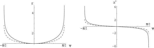
Figure 2: The functions $r(\psi)$ and $x^{3}(\psi)$ for the solutions (B.31) in the interval $\psi\in[-\pi/2,\pi/2]\,\,{\hbox{\rm mod}}\,\,2\pi$. The continuous line represents the embedding with $m=+1$, while the dashed line corresponds to $m=-1$. In this latter case $r(\psi)$ and $x^{3}(\psi)$ remain finite, while for $m=+1$ they diverge at $\psi=\pm\pi/2$.

$$\cos\psi\,=\,{\sinh(2r_{*})\,+\,2m(r-r_{*})\over\sinh(2r)}\,\,,$$ (B.31)

from which it is clear that $r_{*}$ is the value of $r$ such that $\cos\psi=1$. The functions $r(\psi)$ for $m=\pm 1$ written in eq. (B.31), and the corresponding $x^{3}(\psi)$, have been plotted in figure 2. If $m=+1$, the solution (B.31) is such that $r\rightarrow\infty$ and $|x^{3}|\rightarrow\infty$ when $\psi\rightarrow\pm\pi/2\,\,{\hbox{\rm mod}}\,\,2\pi$. However, if $m=-1$ the radial coordinate $r$ grows from its minimal value $r_{*}$ at $\psi=0\,\,{\hbox{\rm mod}}\,\,2\pi$ to a maximal value $\hat{r}\,=\,r_{*}\,+\,{\sinh(2r_{*})\over 2}$ at $\psi=\pm\pi/2\,\,{\hbox{\rm mod}}\,\,2\pi$, while $x^{3}(\psi)$ remains finite when $\psi\in[-\pi/2,\pi/2]\,\,{\hbox{\rm mod}}\,\,2\pi$.

If $C<0$, it is clear from (B.30) that, as we are considering the region $\cos\psi\geq 0$, only the solution with $m=+1$ is possible. Defining $2\tilde{r}=-C$, the solution in this case can be written as

$$\cos\psi\,=\,{2(r-\tilde{r})\over\sinh(2r)}\,\,,\qquad\qquad(m=+1).$$ (B.32)

This solution has two branches such that $r\rightarrow\tilde{r},\infty$ when $\psi\rightarrow\pm\pi/2$. Finally, if $C=0$ only the $m=+1$ solution makes sense. In this case the solution grows from $r=0$ at $\psi=0$ to $r=\infty$ at $\psi=\pm\pi/2$.

In the region $\cos\psi\leq 0$, i.e. for $\psi\in[\pi/2,3\pi/2]\,\,{\hbox{\rm mod}}\,\,2\pi$, the solutions can be found from those for $\cos\psi\geq 0$ by means of the following symmetry of the solution (B.30):

$$\psi\rightarrow\pi-\psi\,\,,\qquad\qquad C\rightarrow-C\,\,,\qquad\qquad m\rightarrow-m\,\,.$$ (B.33)

Then, one can get solutions in the range $\psi\in[0,2\pi]$ by joining one solution in the region $\cos\psi\geq 0$ to the one obtained by means of the transformation (B.33). Notice that the resulting solutions preserve supersymmetry at the cost of changing the angular embedding, i.e. by making $m\rightarrow-m$, when the sign of $\cos\psi$ changes. In particular, in the solution obtained from the one in (B.31) when $m=-1$ the coordinate $r$ does not diverge. One can apply this construction to a single brane probe with a singular embedding or, alternatively, one can consider two different brane probes preserving the same supersymmetry with different angular embeddings and lying on disjoint regions of $\psi$.

B.2 Two-dimensional defects

In analogy with what we have just done with the wall defect solitons, let us find some codimension two embeddings of the D5-brane probe in which the angle $\psi$ is not constant. We shall take the following set of worldvolume coordinates:

$$\xi^{\mu}\,=\,(x^{0},x^{1},r,\theta_{2},\phi_{2},\psi)\,\,,$$ (B.34)

and we will adopt an ansatz in which $x^{2}$ and $x^{3}$ are constant and

$$\theta_{1}=\theta_{1}(\theta_{2}),\,\,\,\,\,\,\,\,\,\,\,\,\,\,\,\phi_{1}=\phi_{1}(\phi_{2}).\,\,\\$$

The induced gamma matrices $\gamma_{x^{\mu}}$ $(\mu=0,1)$, $\gamma_{\theta_{2}}$ and $\gamma_{\phi_{2}}$ are exactly those written in eq. (B.4), while $\gamma_{r}$ and $\gamma_{\psi}$ are given by:

$$e^{-{\phi\over 2}}\,\gamma_{r}\,=\,\Gamma_{r}\,\,,\qquad e^{-{\phi\over 2}}\,\gamma_{\psi}\,=\,{1\over 2}\,\hat{\Gamma}_{3}\,\,.$$ (B.35)

Let us try to implement the kappa symmetry condition in the form displayed in eq. (B.12). For this case, the left-hand side of (B.12) can be written as:

$$e^{-{\alpha\over 2}\,\Gamma_{1}\hat{\Gamma}_{1}}\Gamma_{\kappa}e^{{\alpha\over 2}\,\Gamma_{1}\hat{\Gamma}_{1}}\,\,\epsilon_{0}\,=\,{e^{3\phi}\over 2\sqrt{-g}}\,\,\Gamma_{x^{0}x^{1}}\,\Big{[}\,f_{I}\,+\,f_{1\hat{1}}\,\Gamma_{1}\hat{\Gamma}_{1}\,+\,f_{1\hat{2}}\,\Gamma_{1}\hat{\Gamma}_{2}\,\Big{]}\,\epsilon_{0}\,\,,$$ (B.36)

where the $f$’s are expressed in terms of the ${\cal P}_{i}$ functions of (B.15) as:

$$f_{I}\,=\,\cos\alpha\,{\cal P}_{1}\,+\,\sin\alpha\,{\cal P}_{2}\,\,,$$

$$f_{1\hat{1}}\,=\,-\sin\alpha\,{\cal P}_{1}\,+\,\cos\alpha\,{\cal P}_{2}\,\,,$$

$$f_{1\hat{2}}\,=\,-{\cal P}_{3}\,\,.$$ (B.37)

Since the matrices $\Gamma_{1}\hat{\Gamma}_{1}$ and $\Gamma_{1}\hat{\Gamma}_{2}$ do not commute with the projection (3.48), it is clear that we must impose:

$$f_{1\hat{1}}\,=\,f_{1\hat{2}}\,=\,0\,\,.$$ (B.38)

From the condition $f_{1\hat{1}}\,=\,0$, we get:

$${{\cal P}_{2}\over{\cal P}_{1}}\,=\,\tan\alpha\,\,,$$ (B.39)

while $f_{1\hat{2}}\,=\,0$ is equivalent to the vanishing of ${\cal P}_{3}$, which implies:

$$\sin\theta_{2}\,\partial_{\theta_{2}}\theta_{1}\,=\,\sin\theta_{1}\partial_{\phi_{2}}\phi_{1}\,\,.$$ (B.40)

By using this condition for the angular part of the embedding, we can write the ratio between the functions ${\cal P}_{1}$ and ${\cal P}_{2}$ as:

$${{\cal P}_{2}\over{\cal P}_{1}}\,=\,{r\sin\alpha\,\big{(}\partial_{\theta_{2}}\theta_{1}\big{)}^{2}\over r\cos\alpha\,+\,\Big{(}e^{2h}\,-\,{a^{2}\over 4}\,\Big{)}\Big{(}\big{(}\partial_{\theta_{2}}\theta_{1}\big{)}^{2}-1\Big{)}}\,\,.$$ (B.41)

The consistency between the expressions (B.39) and (B.41) requires that $\partial_{\theta_{2}}\theta_{1}\,=\,\pm 1$. Moreover, by separating variables in the angular embedding equation (B.40) one concludes that $\partial_{\phi_{2}}\phi_{1}=m$ , with $m$ constant. Proceeding as in the previous subsection, one easily verifies that the only consistent solutions of (B.40) with $\partial_{\theta_{2}}\theta_{1}$ constant are:

$$\theta_{1}=\theta_{2}\,\,,\,\,\,\,\,\,\,\,\,\,\,\,\,\,\,\,\,\,\,\,\,\,\,\,\,\,\,\,\,\,\phi_{1}=\phi_{2}\,\,,\,\,\,\,\,\,\,\,\,\,\,\,\,\,\,\,\,\,\,\,\,\,\,\,\,\,\,\,\,\,\,\,\,(m=+1)\,\,,$$

$$\theta_{1}=\pi-\theta_{2}\,\,,\,\,\,\,\,\,\,\,\,\,\,\,\,\,\,\,\,\,\,\,\phi_{2}=2\pi-\phi_{1}\,\,,\,\,\,\,\,\,\,\,\,\,\,\,\,\,\,\,\,\,\,\,(m=-1)\,\,.$$ (B.42)

Notice the difference between (B.42) and (B.23). One can verify that this embedding is a solution of the equations of motion of the probe. Moreover, by computing $\sqrt{-g}$ and $f_{I}$ for the embeddings (B.42), one readily proves that the kappa symmetry condition is equivalent to the following projection on $\epsilon_{0}$:

$$\Gamma_{x^{0}x^{1}}\,\epsilon_{0}\,=\,\epsilon_{0}\,\,.$$ (B.43)

References

- [1] J. M. Maldacena, “The large limit of superconformal field theories and supergravity”, Adv. Theor. Math. Phys. 2 (1998) 231, hep-th/9711200.
- [2] For a review see, O. Aharony, S. Gubser, J. Maldacena, H. Ooguri and Y. Oz, “Large field theories, string theory and gravity”, Phys. Rept. 323 (2000) 183, hep-th/9905111.
-
[3]
J. L. Cardy, “Conformal invariance and surface critical behaviour”,
Nucl. Phys. B240 (1984) 514;
D. M. McAvity and H. Osborn, “Conformal field theories near a boundary in general dimensions”, Nucl. Phys. B455 (1995) 522, cond-mat/9505127. - [4] A. Karch and L. Randall, “Locally localized gravity”, J. High Energy Phys. 0105 (2001) 008, hep-th/0011156; “Open and closed string interpretation of SUSY CFT’s on branes with boundaries”, J. High Energy Phys. 0106 (2001) 063.
- [5] O. DeWolfe, D. Z. Freedman and H. Ooguri, “Holography and defect conformal field theories”, Phys. Rev. D66, 025009 (2002), hep-th/0202056.
- [6] J. Erdmenger, Z. Guralnik and I. Kirsch, “Four-dimensional superconformal theories with interacting boundaries or defects”, Phys. Rev. D66, 025020 (2002), hep-th/0203020.
- [7] K. Skenderis and M. Taylor, “Branes in AdS and pp-wave spacetimes”, J. High Energy Phys. 0206 (2002) 025, hep-th/0204054.
-
[8]
A. Kapustin and S. Sethi, “The Higgs branch of impurity theories”,
Adv. Theor. Math. Phys. 2 (1998) 571,
hep-th/9804027;
D. Tsimpis, “Nahm equations and boundary conditions”, Phys. Lett. B433, 287 (1998), hep-th/9804081. - [9] N. R. Constable, J. Erdmenger, Z. Guralnik and I. Kirsch, “Intersecting D3-branes and holography”, Phys. Rev. D68, 106007 (2003), hep-th/0202056.
-
[10]
A. Fayyazuddin and M. Spalinski, “Large N superconformal gauge
theories and supergravity
orientifolds”,
Nucl. Phys. B535 (1998) 219, hep-th/9805096;
O. Aharony, A. Fayyazuddin and J. M. Maldacena, “The large N limit of field theories from threebranes in F-theory”, J. High Energy Phys. 9807 (1998) 013, hep-th/9806159;
M. Graña and J. Polchinski, “Gauge/gravity duals with holomorphic dilaton”, Phys. Rev. D65 (2002) 126005, hep-th/0106014. - [11] M. Bertolini, P. Di Vecchia, M. Frau, A. Lerda and R. Marotta, “N=2 gauge theories on systems of fractional D3/D7 branes”, Nucl. Phys. B621 (2002) 157, hep-th/0107057.
-
[12]
A. Karch and E. Katz, “Adding flavor to AdS/CFT”,
J. High Energy Phys. 0206 (2002) 043, hep-th/0205236;
A. Karch, E. Katz and N. Weiner, “Hadron masses and screening from AdS Wilson loops”, Phys. Rev. Lett. 90 (2003) 091601, hep-th/0211107. - [13] M. Kruczenski, D. Mateos, R. Myers and D. Winters, “Meson spectroscopy in AdS/CFT with flavour”, J. High Energy Phys. 0307 (2003) 049, hep-th/0304032.
- [14] A. Gorsky and M. A. Shifman, “More on the tensorial central charges in N = 1 supersymmetric gauge Phys. Rev. D61, 085001 (2000) hep-th/9909015
- [15] M. Shifman and A. Yung, “Non-abelian flux tubes in SQCD: Supersizing world-sheet supersymmetry”, hep-th/0501211.
- [16] J. M. Maldacena and C. Núñez, “Towards the large N limit of pure super Yang Mills, Phys. Rev. Lett. 86 (2001) 588, hep-th/0008001.
- [17] A. H. Chamseddine and M. S. Volkov, “Non-Abelian BPS monopoles in gauged supergravity, Phys. Rev. Lett. 79 (1997) 3343, hep-th/9707176; “Non-Abelian solitons in gauged supergravity and leading order string theory”, Phys. Rev. D57 (1998) 6242, hep-th/9711181.
-
[18]
M. Bertolini, “Four lectures on the gauge/gravity
correspondence”, hep-th/0303160;
F. Bigazzi, A. L. Cotrone, M. Petrini and A. Zaffaroni, “Supergravity duals of supersymmetric four dimensional gauge theories”, Riv. Nouvo Cim. 25N12 (2002)1, hep-th/0303191;
E. Imeroni, “The gauge/string correspondence towards realistic gauge theories”, hep-th/0312070;
A. Paredes, “Supersymmetric solutions of supergravity from warpped branes”, hep-th/0407013. - [19] C. Núñez, A. Paredes and A. V. Ramallo, “Flavoring the gravity dual of Yang-Mills with probes”, J. High Energy Phys. 0312 (2003) 024, hep-th/0311201.
- [20] X.-J. Wang and S. Hu, “Intersecting branes and adding flavors to the Maldacena-Núñez background”, J. High Energy Phys. 0309 (2003) 017, hep-th/0307218.
-
[21]
K. Becker, M. Becker and A. Strominger, Fivebranes, membranes and
non-perturbative string theory,
Nucl. Phys. B456 (1995) 130, hep-th/9507158;
E. Bergshoeff, R. Kallosh, T. Ortin and G. Papadopulos, -symmetry, supersymmetry and intersecting branes, Nucl. Phys. B502 (1997) 149, hep-th/9705040;
E. Bergshoeff and P.K. Townsend, Solitons on the supermembrane, J. High Energy Phys. 9905 (1999) 021, hep-th/9904020. -
[22]
M. Cederwall, A. von Gussich, B.E.W. Nilsson, P. Sundell and A.
Westerberg,
The Dirichlet super-p-branes in Type IIA and IIB supergravity,
Nucl. Phys. B490 (1997) 179, hep-th/9611159:
E. Bergshoeff and P.K. Townsend, Super D-branes Nucl. Phys. B490 (1997) 145, hep-th/9611173;
M. Aganagic, C. Popescu and J.H. Schwarz, D-brane actions with local kappa symmetry, Phys. Lett. B393 (1997) 311, hep-th/9610249; Gauge-invariant and gauge-fixed D-brane actions, Nucl. Phys. B495 (1997) 99, hep-th/9612080. -
[23]
I. R. Klebanov, P. Ouyang and E. Witten,
“A gravity dual of the chiral anomaly”,
Phys. Rev. D65, 105007 (2002), hep-th/0202056;
M. Bertolini, P. Di Vechia, M. Frau, A. Lerda and R. Marotta, “More anomalies from fractional branes”, Phys. Lett. B540 (2002)104, hep-th/0202195;
U. Gursoy, S. A. Hartnoll and R. Portugues, “The chiral anomaly from M-theory”, Phys. Rev. D69, 086003 (2004), hep-th/0311088. -
[24]
R. Apreda, F. Bigazzi, A. L. Cotrone, M. Petrini and A. Zaffaroni,
“Some comments on N=1 gauge theories from wrapped branes”,
Phys. Lett. B536 (2002) 161, hep-th/0112236;
P. Di Vecchia, A. Lerda and P. Merlatti, “N=1 and N=2 super Yang-Mills theories from wrapped branes”, Nucl. Phys. B646 (2002) 43, hep-th/0205204. - [25] E. Caceres and C. Nunez, “Glueballs of super Yang-Mills from wrapped branes”, hep-th/0506051.
-
[26]
M. Schvellinger and T. A. Tran,
“Supergravity duals of gauge field theories from gauged supergravity
in five dimensions”,
J. High Energy Phys. 0106 (2001) 025, hep-th/0105019;
J. Maldacena and H. Nastase, “The supergravity dual of a theory with dynamical supersymmetry breaking”, J. High Energy Phys. 0109 (2001) 024, hep-th/0105049;
A. H. Chamseddine and M. S. Volkov, “Non-abelian vacua in D=5, N=4 gauged supergravity, J. High Energy Phys. 0104 (2001) 023, hep-th/0101202. - [27] C. P. Herzog and I. R. Klebanov, “On string tensions in supersymmetric SU(M) gauge theory”, Phys. Lett. B526, 388 (2002) hep-th/0111078.
- [28] S. A. Hartnoll and R. Portugues, “Deforming baryons into confining strings”, Phys. Rev. D70, 066007 (2004) hep-th/0405214.
- [29] J. Gomis, “D-branes, holonomy and M-theory”, Nucl. Phys. B606, 3 (2001), hep-th/0103115.
- [30] B. S. Acharya and C. Vafa, “On domain walls of N = 1 supersymmetric Yang-Mills in four dimensions”, hep-th/0103011.
- [31] J.P. Gauntlett, J. Gomis and P.K. Townsend, BPS bounds for worldvolume branes, J. High Energy Phys. 9801 (1998) 003, hep-th/9711205.
- [32] A. Loewy and J. Sonnenschein, “On the holographic duals of gauge dynamics”, J. High Energy Phys. 0108 (2001) 007, hep-th/0103163;