Fermionic determinant for the SU(N) caloron with nontrivial holonomy

Abstract

In the finite-temperature Yang-Mills theory we calculate the functional determinant for fermions in the fundamental representation of $SU(N)$ gauge group in the background of an instanton with non-trivial holonomy at spatial infinity. This object, called the Kraan–van Baal – Lee–Lu caloron, can be viewed as composed of N Bogomolny–Prasad–Sommerfeld monopoles (or dyons). We compute analytically two leading terms of the fermionic determinant at large separations.

I Introduction

Speaking of the finite temperature one implies that the Euclidean space-time is compactified in the ‘time’ direction whose inverse circumference is the temperature $T$, with the usual periodic boundary conditions for boson fields and anti–periodic conditions for the fermion fields. In particular, it means that the gauge field is periodic in time, and the theory is no longer invariant under arbitrary gauge transformations, but only under gauge transformations that are periodical in time. As the space topology becomes nontrivial the number of gauge invariants increases. The new invariant is the holonomy or the eigenvalues of the Polyakov line that winds along the compact ’time’ direction Polyakov

$$L=\left.{\rm P}\,\exp\left(\int_{0}^{1/T}\!dt\,A_{4}\right)\right|_{|\vec{x}|\to\infty}.$$ (1)

This invariant together with the topological charge and the magnetic charge can be used for the classification of the field configurations GPY , its zero vacuum average is one of the common criteria of confinement.

A generalization of the usual Belavin–Polyakov–Schwartz–Tyupkin (BPST) instantons BPST for arbitrary temperatures is the Kraan–van Baal–Lee–Lu (KvBLL) caloron with non-trivial holonomy KvB ; KvBSUN ; LL . It is a self-dual electrically neutral configuration with topological charge $1$ and arbitrary holonomy. It was constructed a few years ago by Kraan and van Baal KvB and Lee and Lu LL for the SU(2) gauge group and in KvBSUN for the general $SU(N)$ case; it has been named the KvBLL caloron (recently the exact solutions of higher topological charge were constructed and discussed higher ). In the limiting case, when the KvBLL caloron is characterized by the trivial holonomy (meaning that (1) assumes values belonging to the group center $Z(N)$ for the $SU(N)$ gauge group), it reduces to the periodic Harrington-Shepard HS caloron known before. It is purely $SU(2)$ configuration and its weight was studied in detail by Gross, Pisarski and Yaffe GPY .

The KvBLL caloron in the theory with $SU(N)$ gauge group on the space $R^{3}\times S^{1}$ can be interpreted as a composite of $N$ distinct fundamental monopoles (dyons) LY Wein (see fig. 1 and fig. 2). It was proven in KvBSUN and is shown in this paper explicitly, that the exact KvBLL gauge field reduces to a superposition of BPS dyons, when the separation $\varrho_{i}$ between dyons is large (in units of inverse temperature). When the distances $\varrho_{l}$ between all the dyons become small compared to $1/T$ the KvBLL caloron reduces to the usual BPST instanton in its core region (for explicit formulae see KvB ; DG ).

The KvBLL caloron may be relevant to the confinement-deconfinement phase transition in the pure gauge theory DPSUSY as well as for the chiral restoration transition in finite-temperature QCD with light fermions. In the latter case it is important to know the fermionic determinant, which we calculate in this paper.

To construct the ensemble of calorons , one needs to know their quantum weights and moduli space (zero modes). If there are massless fermions in the theory, the “gluonic” quantum weight of the caloron should be multiplied by $\left({\rm Det}^{\prime}(i\nabla/\hskip 3.00003pt)\right)^{N_{f}}$ – a normalized and regularized product of fermionic non-zero modes. The fermionic zero modes would also give a valuable contribution to interactions inside the ensemble.

Up to now, only the determinants in case of the $SU(2)$ gauge group were found. In ref. DGPS the determinant for gluons and ghosts for the $SU(2)$ Yang–Mills theory was computed. It was extended to the SU(2) Yang-Mills theory with light fermions in GS . So far only a metric of the moduli space was known for the general $SU(N)$ case Kraan (its determinant was analyzed in details in DG ). The fermionic zero-modes were studied in Cherndb . In this paper we generalize our results for the fermionic determinant over non-zero modes to the $SU(N>2)$ gauge group. It may be more logical to generalize the result of DGPS about the ghost determinant to the arbitrary $SU(N)$ first, but technically the computation of the non-perturbative contribution of light fermions is simpler and that is why we decided to consider it first.

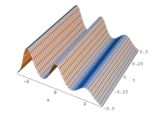
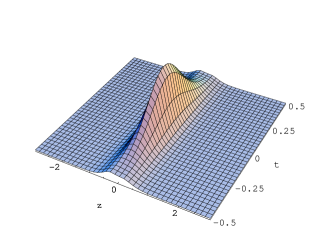
Figure 1: The action density of the $SU(3)$ KvBLL caloron as function of $z,t$ at fixed $x=y=0$, eigenvalues of $A_{4}$ at spatial infinity are $\mu_{1}=-0.307T,\;\mu_{2}=-0.013T,\;\mu_{3}=0.32T$. It is periodic in $t$ direction. At large dyon separation the density becomes static (left, $\varrho_{1,2}=1/T,\;\varrho_{3}=2/T$). As the separation decreases the action density becomes more like a $4d$ lump (right, $\varrho_{1,2}=1/(3T),\;\varrho_{3}=2/(3T)$). The axes are in units of inverse temperature $1/T$.

Let us start a detailed exposition of our calculations. As was already mentioned, to account for fermions we have to multiply the partition function by $\prod\limits_{j=1}^{N_{f}}{\rm Det}(i\nabla/\hskip 3.00003pt+im_{j})$, where $\nabla/\hskip 3.00003pt$ is the spin-1/2 fundamental representation covariant derivative in the background considered, and $N_{f}$ is the number of light flavors. We consider only the case of massless fermions here $m_{j}=0$. The operator $i\nabla/\hskip 3.00003pt$ has zero modes Cherndb therefore a meaningful object is ${\rm Det}^{\prime}(i\nabla/\hskip 3.00003pt)$ — a normalized and regularized product of non-zero modes. In the self-dual background it is equal to $\left({\rm Det}(-\nabla^{2})\right)^{2}$, where $\nabla$ is the spin-0 fundamental covariant derivative BC . In this work we calculate the asymptotics of the determinant for large separations between $N$ constituent dyons. As usual, our method of calculation is based on calculating the variation of the determinant w.r.t. some parameter of the solution Zar .

Let us sketch the structure of the paper. To make the paper more self-contained, in Sections II and III we collect the notations and review the ADHMN construction of $SU(N)$ KvBLL caloron.

A peculiar feature of fields in the fundamental representation of gauge group is that they feel the center elements of the group, hence there are $N$ possible different background fields, numbered by the integer $k=0..N-1$. They are related by a non-periodic gauge transformation (see Section IV.1 for detailes). In Section IV we discuss the $N$ possible background fields and the boundary conditions for the fermionic fluctuations.

In Section VI we present the currents corresponding to variation of the determinant. Using these results we immediately write the result for the determinant up to an additive constant in Section VI. To trace back the constant we shall take a special configuration of N far-separated constituents and will subsequently reduce it to the $SU(2)$ configuration, where we have already calculated the determinant in GS . To justify this approach we show rigorously in Section IV that the $SU(N)$ caloron can be considered as a superposition of $SU(2)$ dyons and explicitly show how some degenerate $SU(N)$ configurations are reduced to the $SU(N-1)$ ones. The simplicity of formulae appearing in the main text is justified by rigorous and lengthy calculations presented in Appendices. We also prove several statements conjectured numerically in our previous works DGPS ; GS .

II Notations

To help navigate and read the paper, we first introduce some notations used throughout. Basically we use the same notations as in Ref. KvBSUN . In what follows we shall measure all quantities in the temperature units and put $T=1$. The temperature factors can be restored in the final results from dimensions.

Let the holonomy at spatial infinity have the following eigenvalues

$$L={\rm P}\,\exp\left(\int_{0}^{1/T}\!dt\,A_{4}\right)_{|\vec{x}|\to\infty}=V\,{\rm diag}\left(e^{2\pi i\mu_{1}},\,e^{2\pi i\mu_{2}}\ldots e^{2\pi i\mu_{N}}\right)\,V^{-1},\qquad\sum_{m=1}^{N}\mu_{m}=0.$$ (2)

We use anti-hermitian gauge fields $A_{\mu}=it^{a}A_{\mu}^{a}=\frac{i}{2}\lambda^{a}A_{\mu}^{a}$, $[t^{a}t^{b}]=if^{abc}t^{c},\,{\rm tr}(t^{a}t^{b})=\frac{1}{2}\delta^{ab}$. The eigenvalues $\mu_{m}$ are uniquely defined by the condition $\sum_{m=1}^{N}\mu_{m}=0$. If all eigenvalues are equal up to the integer, implying $\mu_{m}=k/N-1,\;m\leq k$ and $\mu_{m}=k/N,\;m>k$ where $k=0,1,...(N-1)$, the holonomy belongs to the center of $SU(N)$ group, and is said to be “trivial”. By making a global gauge rotation one can always order the holonomy eigenvalues such that

$$\mu_{1}\leq\mu_{2}\leq\ldots\leq\mu_{N}\leq\mu_{N+1}\equiv\mu_{1}+1,$$ (3)

which we shall assume done. The eigenvalues of $A_{4}$ in the adjoint representation, $A_{4}^{ab}=if^{abc}A_{4}^{c}$, are $\pm(\mu_{m}-\mu_{n})$ and $N-1$ zero ones. For the trivial holonomy all the adjoint eigenvalues are integers. The difference between the neighboring eigenvalues in the fundamental representation $\nu_{m}\equiv\mu_{m+1}-\mu_{m}$ determines the spatial core size $1/\nu_{m}$ of the $m^{\rm th}$ monopole whose 3-coordinates will be denoted as $\vec{y}_{m}$, and the spatial separation between neighboring monopoles will be denoted by

$$\vec{\varrho}_{m}\equiv\vec{y}_{m}-\vec{y}_{m-1}=\varrho_{m}\,(\sin\theta_{m}\cos\phi_{m},\,\sin\theta_{m}\sin\phi_{m},\,\cos\theta_{m}),\qquad\varrho_{m}\equiv|\vec{\varrho}_{m}|.$$ (4)

We call neighbors those dyons which correspond to the neighboring intervals in $z$ variable (see the next section), these dyons also turn out to be neighbors in the color space. With each 3-vector $\vec{\varrho}_{m}$ we shall associate a 2-component spinor $\zeta^{\dagger\,\alpha}_{m}$ so that for any $m=1...N$:

$$\zeta^{\dagger\,\alpha}_{m}\zeta^{m}_{\beta}=\frac{1}{2\pi}\left(1_{2}\varrho_{m}-\vec{\tau}\cdot\vec{\varrho}_{m}\right)^{\alpha}_{\beta}\,.$$ (5)

This condition defines $\zeta_{m}^{\alpha}$ up to $N$ phase factors $e^{i\psi_{m}/2}$. These spinors are used in the construction of the caloron field. These $\psi_{m}$ has the meaning of the $U(1)$ phase of the $m^{\rm th}$ dyon. For the trivial holonomy, the KvBLL caloron reduces to the Harrington–Shepard periodic instanton at non-zero temperatures and to the ordinary Belavin–Polyakov–Schwartz–Tyupkin instanton at zero temperature. Instantons are usually characterized by the scale parameter (the “size” of the instanton) $\rho$. It is directly related to the dyons positions in space, actually to the perimeter of the polygon formed by dyons,

$$\rho=\sqrt{\frac{1}{2\pi T}\sum_{m=1}^{N}\varrho_{m}}\,,\qquad\sum_{m=1}^{N}\vec{\varrho}_{m}=0.$$ (6)

In the next Section we shall show how the $SU(N)$ caloron gauge field depends on these parameters and describe its ADHMN construction.

Figure 2: The action density of the $SU(3)$ KvBLL caloron as function of $z,x$ at fixed $t=y=0$. At large separations $\varrho_{1,2,3}$ the caloron is a superposition of free BPS dyon solutions (left, $\varrho_{1}=2.8/T,\;\varrho_{2,3}=2/T$). At small separations they merge (right, $\varrho_{1}=1/T,\;\varrho_{2,3}=0.54/T$). The eigenvalues of $A_{0}$ at spatial infinity are the same as in Fig. 1.

III ADHMN construction for the SU(N) caloron

Here we remind the Atiyah–Drinfeld–Hitchin–Manin–Nahm (ADHMN) construction for the $SU(N)$ caloron KvBSUN and adjust it to our needs.

The basic object in the ADHMN construction ADHM ; Nahm80 is the $(2+N)\times 2$ matrix $\Delta$ linear in the space-time variable $x$ and depending on an additional compact variable $z$ belonging to the unit circle:

$$\Delta^{K}_{\beta}(z,x)=\left\{\begin{array}[]{cl}\lambda^{m}_{\beta}(z)&,\quad K=m,\quad 1\leq m\leq N,\\ (B(z)-x_{\mu}\sigma_{\mu})^{\alpha}_{\beta}&,\quad K=N+\alpha,\quad 1\leq\alpha\leq 2,\end{array}\right.$$ (7)

where $\alpha,\beta=1,2$ and $m=1,\dots,N$; $\sigma_{\mu}=(i\vec{\sigma},1_{2})$. As usual, the superscripts number rows of a matrix and the subscripts number columns. The functions $\lambda^{m}_{\beta}(z)$ forming an $N\times 2$ matrix carry information about color orientations of the constituent dyons, encoded in the $N$ two-spinors $\zeta$:

$$\lambda^{m}_{\beta}(z)=\delta(z-\mu_{m})\zeta^{m}_{\beta}.$$ (8)

The quantities $\zeta^{m}_{\beta}$ transform as contravariant spinors of the gauge group $SU(N)$ but as covariant spinors of the spatial $SU(2)$ group. The $2\times 2$ matrix $B$ is a differential operator in $z$ and depends on the positions of the dyons in the $3d$ space $\vec{y}_{m}$ and the overall position in time $\xi_{4}=x_{4}$:

$$B^{\alpha}_{\beta}(z)=\frac{\delta^{\alpha}_{\beta}\partial_{z}}{2\pi i}+\frac{\hat{A}^{\alpha}_{\beta}(z)}{2\pi i}$$ (9)

with

$$\hat{A}(z)=A_{\mu}\sigma_{\mu},\qquad\vec{A}(z)=2\pi i\,\vec{y}_{m}(z),\qquad A_{4}=2\pi i\,\xi_{4},$$ (10)

where for $z$ inside the interval $\mu_{m}\leq z\leq\mu_{m+1}$, we define $\vec{y}(z)=\vec{y}_{m}$ to be the position of the $m^{\rm th}$ dyon with the inverse size $\nu_{m}\equiv\mu_{m+1}-\mu_{m}$.

The gauge field of the caloron can be constructed in the following way. One has to find $N$ quantities $v^{K}_{n}(x),\,n=1...N,$

$$v^{K}_{n}(x)=\left\{\begin{array}[]{cl}v^{1m}_{n}(x)&,\quad K=m,\quad 1\leq m\leq N,\\ v^{2\alpha}_{n}(z,x)&,\quad K=N+\alpha,\quad 1\leq\alpha\leq 2,\end{array}\right.$$ (11)

which are normalized independent solutions of the differential equation

$${\lambda^{\dagger}}^{\alpha}_{m}(z)v^{1m}_{n}+[B^{\dagger}(z)-x_{\mu}\sigma^{\dagger}_{\mu}]^{\alpha}_{\beta}v^{2\beta}_{n}(z,x)=0,\qquad v^{{\dagger}1m}_{l}\,v^{1l}_{n}+\int_{-1/2}^{1/2}dz\,v^{{\dagger}2m}_{\alpha}\,v^{2\alpha}_{n}=\delta^{m}_{n}\,,$$ (12)

or, in short hand notations,

$$\Delta^{\dagger}v=0,\qquad v^{\dagger}v=1_{N}.$$ (13)

Note that only the lower component $v^{2}$ depends on $z$. Once $v^{1,2}$ are found, the caloron gauge field $A_{\mu}$ is an anti-Hermitian $N\times N$ matrix whose matrix elements are simply

$$\left(A_{\mu}\right)^{m}_{n}=v^{{\dagger}1m}_{l}\,\partial_{\mu}v^{1l}_{n}+\int_{-1/2}^{1/2}dz\,v^{{\dagger}2m}_{\alpha}\,\partial_{\mu}v^{2\alpha}_{n}\qquad{\rm or}\quad A_{\mu}=v^{\dagger}\partial_{\mu}v.$$ (14)

The gauge field is self-dual if

$$(\Delta^{\dagger}\Delta)^{\alpha}_{\beta}\propto\delta^{\alpha}_{\beta}.$$ (15)

It is important that there is a $U(1)$-internal gauge freedom. For an arbitrary function $U(z)$, such that $|U(z)|=1$ a new operator

$$\Delta^{K}_{U,\beta}(z,x)=\left\{\begin{array}[]{cl}\lambda(z)^{m}_{\beta}U(z)&,\;\;\;\;\;K=m,\quad 1\leq m\leq N,\\ U^{\dagger}(z)(B(z)-x)^{\alpha}_{\beta}U(z)&,\;\;\;\;\;K=N+\alpha,\quad 1\leq\alpha\leq 2,\end{array}\right.$$ (16)

can be equally well used in the construction above.

III.0.1 ADHM Green’s function

One can define the scalar ADHMN Green function satisfying

$$(\Delta^{\dagger}\Delta)^{\alpha}_{\beta}f(z,z^{\prime})=\delta^{\alpha}_{\beta}\,\delta(z-z^{\prime}).$$ (17)

From eq.(15) one can deduce that the $N$ two-spinors $\zeta^{m}_{\alpha}$ defined in eq.(8) are associated with $\vec{\varrho}_{m}\equiv\vec{y}_{m}-\vec{y}_{m-1}$ according to eq.(5).

Eq.(17) is in fact a Shrödinger equation on the unit circle:

$$\left[\left(\frac{1}{2\pi i}\partial_{z}-x_{0}\right)^{2}+r(z)^{2}+\frac{1}{2\pi}\sum_{m}\delta(z-\mu_{m})\varrho_{m}\right]f(z,z^{\prime})=\delta(z-z^{\prime})$$ (18)

where $r(z)\equiv|\vec{x}-\vec{y}(z)|$. This equation can be solved by means of different methods multicaloron . We shall use the solution in the form found in DG

$$f(z,z^{\prime})=s_{m}(z)f_{mn}s^{{\dagger}}_{n}(z^{\prime})+2\pi s(z,z^{\prime})\delta_{[z][z^{\prime}]}$$ (19)

we denoted $[z]\equiv m$ if $\mu_{m}\leq z<\mu_{m+1}$. The functions appearing in eq.(19) are

$$s_{m}(z) = e^{2\pi ix_{0}(z-\mu_{m})}\frac{\sinh[2\pi r_{m}(\mu_{m+1}-z)]}{\sinh(2\pi r_{m}\nu_{m})}\delta_{m[z]}+e^{2\pi ix_{0}(z-\mu_{m})}\frac{\sinh[2\pi r_{m-1}(z-\mu_{m-1})]}{\sinh(2\pi r_{m-1}\nu_{m-1})}\delta_{m,[z]+1},$$ (20)

$$s(z,z^{\prime}) = e^{2\pi ix_{0}(z-z^{\prime})}\frac{\sinh\!\left(2\pi r_{[z]}(\min\{z,z^{\prime}\}-\mu_{[z]})\right)\sinh\!\left(2\pi r_{[z]}(\mu_{[z]+1}-\max\{z,z^{\prime}\})\right)}{r_{[z]}\sinh\!\left(2\pi r_{[z]}\nu_{[z]}\right)}.$$ (21)

In fact $s(z,z^{\prime})$ is a single dyon Green’s function. $N\times N$ matrix $f_{nm}=f(\mu_{n},\mu_{m})$ is defined by its inverse $f_{mn}={F^{-1}}_{mn}$

$$2\pi F_{mn}=\delta_{mn}\left[\coth(2\pi r_{m}\nu_{m})r_{m}+\coth(2\pi r_{m-1}\nu_{m-1})r_{m-1}+\varrho_{m}\right]-\frac{\delta_{m+1,n}r_{m}e^{-2\pi ix_{0}\nu_{m}}}{\sinh(2\pi r_{m}\nu_{m})}-\frac{\delta_{m,n+1}r_{n}e^{2\pi ix_{0}\nu_{n}}}{\sinh(2\pi r_{n}\nu_{n})}\,.$$ (22)

Eq.(19) is convenient since the main dependence on $z,z^{\prime}$ is factorized. Moreover a single dyon limit is manifested.

III.0.2 Projector

An important quantity frequently used in the ADHM calculus is the projector

$$P\equiv vv^{\dagger}=1-\Delta f\Delta^{\dagger}$$ (23)

or, writing all indices explicitly,

$$P^{K}_{L}=\left\{\begin{array}[]{cl}(P^{11})^{m}_{n}=v^{1m}_{l}\,v^{{\dagger}1l}_{n}&,\quad K=m,\quad L=n;\\ (P^{12})^{m}_{\beta}(z^{\prime})=v^{1m}_{l}\,v^{{\dagger}2l}_{\beta}(z^{\prime})&,\quad K=m,\quad L=N+\beta;\\ (P^{21})^{\alpha}_{n}(z)=v^{2\alpha}_{l}(z)\,v^{{\dagger}1l}_{n}&,\quad K=N+\alpha,\quad L=n;\\ (P^{22})^{\alpha}_{\beta}(z,z^{\prime})=v^{2\alpha}_{l}(z)\,v^{{\dagger}2l}_{\beta}(z^{\prime})&,\quad K=N+\alpha,\quad L=N+\beta.\end{array}\right.$$ (24)

Eq.(23) states that

$$(P^{11})^{m}_{n}=\delta^{m}_{n}-\zeta^{m}_{\alpha}f(\mu_{m},\mu_{n})\zeta^{{\dagger}\alpha}_{n}, \quad(P^{12})^{m}_{\beta}(z^{\prime})=-\zeta^{m}_{\alpha}f(\mu_{m},z^{\prime})[B^{\dagger}(z^{\prime})-x^{\dagger}]^{\alpha}_{\beta},$$

$$(P^{21})^{\alpha}_{n}(z)=-[B(z)-x]^{\alpha}_{\beta}f(z,\mu_{n})\zeta^{{\dagger}\beta}_{m}, \quad(P^{22})^{\alpha}_{\beta}(z,z^{\prime})=\delta^{\alpha}_{\beta}\delta(z-z^{\prime})-[B(z)-x]^{\alpha}_{\gamma}f(z,z^{\prime})[B^{\dagger}(z^{\prime})-x^{\dagger}]^{\gamma}_{\beta}\,.$$ (25)

It is easy to see from eq.(17) that both sides are projectors onto the kernel of $\Delta^{\dagger}$:

$$(vv^{\dagger})^{2}=vv^{\dagger},\;\;\;\;\;(1-\Delta f\Delta^{\dagger})^{2}=1-\Delta f\Delta^{\dagger},\;\;\;\;\;{P}v=v.$$ (26)

III.0.3 Gauge field through $f_{mn}$

It was shown by Kraan and van Baal KvBSUN that instead of eq.(14) one can use:

$$A^{mn}_{\mu}=\frac{1}{2}\phi_{mk}^{1/2}\zeta^{k}_{\alpha}\bar{\eta}^{a}_{\mu\nu}(\tau^{a})^{\alpha}_{\beta}\zeta^{{\dagger}\,\beta}_{l}\partial_{\nu}f_{kl}\phi_{ln}^{1/2}+\frac{1}{2}\left(\phi^{1/2}_{mk}\partial_{\mu}\phi_{kn}^{-1/2}-\partial_{\mu}\phi_{mk}^{-1/2}\phi_{kn}^{1/2}\right)$$ (27)

where

$${\phi^{-1}}_{mn}=\delta_{mn}-\zeta^{m}_{\alpha}f_{mn}\zeta^{{\dagger}\,\alpha}_{n}\,.$$ (28)

We see that only $f_{mn}\equiv f(\mu_{m},\mu_{n})$ is needed to calculate $A_{\mu}$.

IV KvBLL caloron gauge field, basic features

IV.1 Periodicity of the KvBLL caloron

From eq.(27) one can see that $A_{\mu}$ is not periodical in time as it should be. More explicitly for any integer $k$

$$A_{\mu}(x_{0}+k,\vec{x})=g(k)A_{\mu}(x_{0},\vec{x})g^{\dagger}(k)\;$$ (29)

where $g$ is a diagonal matrix $g_{mn}(k)=\delta_{mn}e^{2\pi ik\mu_{n}}$. To prove (29) it is enough to see from (22) that for integer $k$

$$f_{mn}(k,\vec{x})=f_{mn}(0,\vec{x})e^{2\pi ik(\mu_{m}-\mu_{n})}\;.$$ (30)

Now we can easily make the gauge field periodic by making a time dependent gauge transformation

$$A^{\rm per}_{\mu}=g^{\dagger}(x_{0})\partial_{\mu}g(x_{0})+g^{\dagger}(x_{0})A_{\mu}g(x_{0}).$$ (31)

However this is not the only possibility to make the field periodic in time. Instead of $g(x_{0})$ one can use $g_{k}(x_{0})\equiv\exp[x_{0}{\rm diag}(2\pi i(\mu_{1}+k/N),\dots,2\pi i(\mu_{N}+k/N-1))]$ as $g(n)g^{\dagger}_{k}(n)\in{\mathbb{Z}}_{N}$ is an element of the center of the $SU(N)$ gauge group. Correspondingly we denote

$$A^{k}_{\mu}=g_{k}^{\dagger}(x_{0})\partial_{\mu}g_{k}(x_{0})+g_{k}^{\dagger}(x_{0})A_{\mu}g_{k}(x_{0})$$ (32)

For different $k$, the $A^{k}_{\mu}$ cannot be related by a periodical gauge transformation. In particular the fermionic determinant depends explicitly on a particular choice of $k=0,\dots,N-1$. However the expressions for $A_{\mu}^{k}$ are related as it is shown in Appendix A.

IV.2 KvBLL caloron with exponential precision

The caloron gauge field (27) has an important feature: it is abelian with the exponential precision, i.e. neglecting terms of the type $e^{-2\pi\mu_{i}r_{i}}$ and $e^{-2\pi\nu_{i}r_{i}}$ one obtains DG in the periodical gauge (31)

$$A_{4\,mn} = 2\pi i\mu_{m}\delta_{mn}+\frac{i}{2}\delta_{mn}\left(\frac{1}{r_{m}}-\frac{1}{r_{m-1}}\right),$$ (33)

$$\vec{A}_{mn} = -\frac{i}{2}\delta_{mn}\left(\frac{1}{r_{m}}+\frac{1}{r_{m-1}}\right)\sqrt{\frac{(\varrho_{m}-r_{m}+r_{m-1})(\varrho_{m}+r_{m}-r_{m-1})}{(\varrho_{m}+r_{m}+r_{m-1})(r_{m}+r_{m-1}-\varrho_{m})}}\;\;\vec{e}_{\varphi_{m}}$$

where $\vec{e}_{\varphi_{m}}\equiv\frac{\vec{r}_{m-1}\times\vec{r}_{m}}{|\vec{r}_{m-1}\times\vec{r}_{m}|}$.

IV.3 Reduction to a single BPS dyon

In KvBSUN it was shown that in the domain near the $l$-th dyon where $r_{l}\ll r_{n}$ for all $n\neq l$ and the perimeter $\sum_{n}\varrho_{n}\gg 1$ is large, the action density of the KvBLL caloron reduces to that of a single dyon (with the ${\cal O}(1/r_{n})$ precision). Note that the cores of dyons may overlap and in particular when one dyon blows up and its size $1/\nu_{l}$ tends to infinity all the other dyons do not lose their shape. We will use this fact to calculate the constant in the resulting expression for the determinant.

In Appendix C we show explicitly how the KvBLL caloron looks like in the vicinity of a dyon for the case of well-separated constituents (i.e. when $e^{\nu_{n}r_{n}}\gg 1$ for all $n\neq i$ ).

IV.4 Reduction to the $SU(N-1)$ configuration

In this Section we will show that the $SU(N)$ caloron gauge field can be continuously deformed into an $SU(N-1)$ one. This fact allows one to calculate the determinant by induction as the determinant for the $SU(2)$ gauge group is known GS .

Let us consider an $SU(N)$ caloron when the size of the $l$-th dyon becomes infinite (or $\nu_{l}=0$, meaning $\mu_{l}=\mu_{l+1}$). We shall prove that when the center of the “disappeared” dyon $l$ is lying on the straight line connecting the two neighboring dyons $l-1$ and $l+1$, the resulting configuration is an $SU(N-1)$ caloron solution having the same dyon content (except the $l$-th one) at the same positions in space. In KvBSUN this statement was verified for the action density. Here we show this explicitly for the gauge field and find the gauge transformation that imbeds the $SU(N-1)$ gauge field into the upper-left $(N-1)\times(N-1)$ block of the $SU(N)$ matrix.

It is easy to see from the definition of the Green’s function (18) that at $\nu_{l}=0$ one has $f_{ln}=f_{{l+1}n},\;f_{nl}=f_{n{l+1}}$. Let us denote with tilde the elements of the $SU(N-1)$ construction. One can see from the definition (18) that

$$\tilde{f}_{nm}=f_{nm},\;\;\;\;\; n,m\leq l,$$

$$\tilde{f}_{nm}=f_{n+1m+1},\;\;\;\;\; n,m>l,$$

$$\tilde{f}_{nm}=f_{n+1m},\;\;\;\;\; n>l,\;m\leq l,$$

$$\tilde{f}_{nm}=f_{nm+1},\;\;\;\;\; m>l,\;n\leq l\;.$$

Since $\vec{\varrho}_{l}$ and $\vec{\varrho}_{l+1}$ are parallel one can write

$$\tilde{\zeta}_{n}^{\alpha}=\zeta_{n}^{\alpha},\;\;\;\;\; n<l$$

$$\tilde{\zeta}_{n}^{\alpha}=\zeta_{n+1}^{\alpha},\;\;\;\;\; n>l$$

$$\tilde{\zeta}_{l}^{\alpha}=\sqrt{\frac{\varrho_{l}+\varrho_{l+1}}{\varrho_{l}}}\zeta_{l}^{\alpha},$$

and this is consistent with the constraint (5).

Let us write down explicitly the gauge transformation relating the $SU(N)$ and the $SU(N-1)$ constructions. The crucial point is the following identity

$$\zeta^{n}_{\alpha}f_{nm}{\zeta^{\dagger}}_{m}^{\beta}=(U^{\dagger}\tilde{\zeta}_{\alpha}\tilde{f}\tilde{\zeta}^{{\dagger}\beta}U)_{nm}$$ (36)

where $U$ is a unitary matrix given by

$$U_{mn}=\delta_{mn},\;\;\;\;\; m<l$$

$$U_{mn}=\delta_{mn+1},\;\;\;\;\; m>l+1$$

$$U_{ln}=\delta_{ln}\sqrt{\frac{\varrho_{l}}{\varrho_{l}+\varrho_{l+1}}}-\delta_{Nn}\sqrt{\frac{\varrho_{l+1}}{\varrho_{l}+\varrho_{l+1}}}$$

$$U_{l+1n}=\delta_{ln}\sqrt{\frac{\varrho_{l+1}}{\varrho_{l}+\varrho_{l+1}}}+\delta_{Nn}\sqrt{\frac{\varrho_{l}}{\varrho_{l}+\varrho_{l+1}}}$$

It is assumed here that the $SU(N-1)$ construction in context of the $SU(N)$ construction is simply appended with zeroes at the end to get the needed matrix size. Since the gauge field (27) is expressed entirely through the combination (36), $U$ is a unitary gauge transformation matrix that transforms $SU(N)$ configuration given by eq.(27) into $SU(N-1)$ configuration given by the same eq.(27). We see that $\zeta_{l}$ is consistently determined in terms of other N-1 $\zeta$’s thus reducing by 4 the number of independent degrees of freedom.

V Method of computation

In calculating the small oscillation determinant, ${\rm Det}(-\nabla^{2})$, where $\nabla_{\mu}=\partial_{\mu}+A_{\mu}$ and $A_{\mu}$ is the $SU(N)$ caloron field KvBSUN in the fundamental representation, we employ the same method as in GS ; DGPS ; Zar . Instead of computing the determinant directly, we first evaluate its derivative with respect to a parameter $\cal P$, and then integrate the derivative using the known determinant for the $SU(2)$ case. In case of fermions one should consider the determinant over anti-periodical fluctuations. In Appendix A we consider a more general problem with fluctuations periodical up to the phase factor $e^{i\tau}$, and calculate the dependence of the determinant on $\tau$. However for simplicity we can put $\tau=0$, i.e. consider periodical fluctuations. The dependence on $\tau$ will be restored in the final result with the help of Appendix A. Moreover, let us note that the dependence of the determinant on the parameter $k$ of the gauge field (see (32)) is the same as the dependence on $\tau$ ($k$ can be absorbed in $\tau$ as $\tau\to\tau+2\pi k/N$ or vice versa).

If the background field $A_{\mu}$ depends on some parameter ${\cal P}$, a general formula for the derivative of the determinant with respect to ${\cal{P}}$ is

$$\frac{\partial\,\log{\rm Det}(-\nabla^{2}[A])}{\partial{\cal P}}=\!-\!\int d^{4}x\,{\rm Tr}\left(\partial_{\cal P}A_{\mu}\,J_{\mu}\right)$$ (38)

where $J_{\mu}$ is the vacuum current in the external background, determined by the Green function:

$$J^{ab}_{\mu}\!\equiv\!\left.(\delta^{a}_{c}\delta^{b}_{d}\partial_{x}\!-\!\delta^{a}_{c}\delta^{b}_{d}\partial_{y}\!+\!A^{ac}\delta^{b}_{d}\!+\!A^{db}\delta^{a}_{c}){\cal G}^{cd}(x,y)\right|_{y=x}\qquad{\rm or\;simply}\quad J_{\mu}\equiv\overrightarrow{\nabla}_{\mu}{\cal G}+{\cal G}\overleftarrow{\nabla}_{\mu}.$$ (39)

Here $\cal G$ is the Green’s function or the propagator of spin-0, fundamental representation particle in the given background $A_{\mu}$, defined by

$$-\nabla^{2}_{x}G(x,y)=\delta^{(4)}(x-y).$$ (40)

The periodic propagator can be easily obtained from it by a standard procedure:

$${\cal G}(x,y)=\sum_{n=-\infty}^{+\infty}G(x_{4},{\vec{x}};y_{4}+n,{\vec{y}}).$$ (41)

Eq.(38) can be verified by differentiating the identity $\log{\rm Det}(-D^{2})={\rm Tr}\log(-D^{2})$. The background field $A_{\mu}$ in eq.(38) is taken in the fundamental representation, as is the trace.

The Green functions in the self-dual backgrounds are generally known CWS ; Nahm80 and are built in terms of the Atiyah–Drinfeld–Hitchin–Manin (ADHM) construction ADHM

$$G(x,y)=\frac{v^{\dagger}(x)v(y)}{4\pi^{2}(x-y)^{2}}\;.$$ (42)

In what follows it will be convenient to split it into two parts:

$${\cal G}(x,y) = {\cal G}^{\rm r}(x,y)+{\cal G}^{\rm s}(x,y),$$

$${\cal G}(x,y)^{\rm s}\equiv G(x,y), \qquad{\cal G}(x,y)^{\rm r}\equiv\sum\limits_{n\neq 0}G(x_{4},{\vec{x}};y_{4}+n,{\vec{y}})\;.$$ (43)

The vacuum current (39) can be also split into two parts, “singular” and “regular”, in accordance to which part of the periodic propagator (43) is used to calculate it:

$$J_{\mu}=J^{\rm r}_{\mu}+J^{\rm s}_{\mu}.$$ (44)

Note that if we leave only $J^{\rm s}_{\mu}$ in the r.h.s. of eq.(38) then in the l.h.s. we will get a derivative of the logarithm of the determinant over all fluctuations (not only periodical). Therefore both

$$\int d^{4}x\;{\rm Tr}(\delta A_{\mu}J^{\rm s}_{\mu})\;\;\;\;\;{\rm and}\;\;\;\;\;\int d^{4}x\;{\rm Tr}(\delta A_{\mu}J^{\rm r}_{\mu})$$ (45)

are full variations of certain functional $F^{\rm s}[A],\;F^{\rm r}[A]$, such that

$$\frac{\partial\,\log{\rm Det}(-\nabla^{2}[A])}{\partial{\cal P}}=\partial_{\cal P}F^{\rm s}[A]+\partial_{\cal P}F^{\rm r}[A].$$ (46)

By definition $F^{\rm s}[A]$ is the determinant over arbitrary fluctuations. This defines uniquely $F^{\rm r}[A]$. In fact $F^{\rm r}[A]$ is particularly simple and it is calculated exactly in Appendix B. The result is simply

$$F^{\rm r}[A]=\sum_{n}\left(P^{\prime\prime}(2\pi\mu_{n})\frac{\pi\varrho_{n}}{4}-P^{\prime}(2\pi\mu_{n})\frac{\pi}{6}(y_{n}^{2}-y_{n-1}^{2})+P(2\pi\mu_{n})\frac{V}{2}\right),$$ (47)

where $V$ is the space volume, $P({\rm v})={\rm v}^{2}(2\pi-{\rm v})^{2}/(12\pi^{2})$ is the 1-loop effective potential GPY ; NW . In the $SU(2)$ case this simple exact expression was conjectured in GS from numerical results. In this paper we prove it analytically for any $SU(N)$, see Appendix B.

As for $F^{\rm s}[A]$, we are only able to calculate this quantity for large dyon separations. The method is the same as in DGPS ; GS . We divide the space into the “core” and “far” domains. The first contains well separated dyons and consists of $N$ balls of radius $R\ll 1/\nu_{n}$. In the core region the r.h.s. of eq.(38) is given by the simple expression computed on a single BPS dyon with the ${\cal O}(1/\varrho_{n})$ precision. In the far domain the r.h.s. of eq.(38) can be computed with exponential precision. The calculations are presented in the next section.

VI Determinant at large separations between dyons

Let us consider the range of the moduli space, where the dyon cores do not overlap. To calculate the variation of the determinant, it is convenient to divide the space into N core domains (N balls of radius $R\gg 1/\nu_{n}$), and the remaining far region. Integrating the total variation of the determinant we shall get the determinant up to the constant that does not depend on the caloron parameters since the considered region in the moduli space is connected.

VI.1 Core domain

In this section we calculate the r.h.s. of eq.(38) in the vicinity of the $m^{\rm th}$ dyon center. As the distances to other dyons are large we can use simple formulae obtained for a single BPS dyon in GS . We only have to make a remark that in GS the calculations were made in the periodical gauge. In the present case the gauge is not periodical. From eq.(114) one can see that we have to make a $U(1)$ non-periodical gauge transformation (this results in adding a constant proportional to a unit $2\times 2$ matrix to the BPS gauge field, see eq.(115)) and thus naively the formulae are not applicable. However in Appendix A it is shown that only the IR-infinite terms change under this $U(1)$ transformation (i.e. $R$-dependent terms) and the main IR-finite part that contributes to the caloron determinant is the same. We can conclude that the single dyon determinant depends nontrivially only on $\nu_{m}=\mu_{m+1}-\mu_{m}$. All other changes affect only the IR-infinite terms:

$$\partial_{{\cal P}}\log{\rm Det}(-D^{2})_{\rm near\;m^{th}\;dyon} = \partial_{\cal P}\left(c_{dyon}\nu_{m}-\frac{\log(\nu_{m}R)}{6}\nu_{m}\right)+(R{\rm-dependent\;terms})$$ (48)

where ${\cal P}=\mu_{n}$ or $\vec{y}_{n}$. Adding up all core contributions we obtain

$$\partial_{\cal P}\log{\rm Det}_{{\rm core}}(-D^{2})=-\partial_{\cal P}\left(\sum_{n}\frac{\nu_{n}\log(\nu_{n}R)}{6}\right)+(R{\rm-dependent\;terms}).$$ (49)

The constant $c_{dyon}$ has disappeared here because $\sum\nu_{m}=1$, and so it does not enter the variation. $R$-dependent terms are exactly cancelled when we sum with the far region contribution, since the total result cannot depend on the choice of $R$.

VI.2 Far domain

Now we consider the far domain, i.e. the region of space outside dyons’ cores. We need to compute the vacuum current (39) with exponential precision. However in fact we can obtain the result instantly using the fact that the gauge field is diagonal with the same precision, and for all $\mu_{n}\neq 0$ the Green’s function (41) falls off exponentially and thus the result can be read off from the $SU(2)$ one. For periodical boundary conditions we have

$$j_{4}^{mn}=\delta_{mn}\frac{i{\rm s}_{m}}{2}P^{\prime}\left[\frac{1}{2}\left(4\pi\mu_{m}+\frac{1}{r_{m}}-\frac{1}{r_{m-1}}\right)\right],$$ (50)

where ${\rm s}_{m}=\frac{\mu_{m}}{|\mu_{m}|}$. All the other components are zero with exponential precision. We have also checked this by a direct computation. It is rather involved and we do not include it in this paper. We can immediately conclude from eq.(33) for the gauge field that

$$\partial_{\cal P}\log{\rm Det}_{{\rm far}}(-D^{2})=\int_{far}\partial_{\cal P}\frac{1}{2}\sum_{n}P\left[\frac{1}{2}\left(4\pi\mu_{n}+\frac{1}{r_{n}}-\frac{1}{r_{n-1}}\right)\right]$$ (51)

$$=\partial_{\cal P}\sum_{n}\left(P^{\prime\prime}(2\pi\mu_{n})\frac{\pi\varrho_{n}}{4}-P^{\prime}(2\pi\mu_{n})\frac{\pi}{6}(y_{n}^{2}-y_{n-1}^{2})+P(2\pi\mu_{n})\frac{V}{2}\right)+(R{\rm-dependent\;terms}).$$

We have used

$$\int\left(\frac{1}{r_{n}}-\frac{1}{r_{n-1}}\right)d^{3}x=\frac{2\pi}{3}(y_{n-1}^{2}-y_{n}^{2}),\;\;\;\;\;\int\left(\frac{1}{r_{n}}-\frac{1}{r_{n-1}}\right)^{2}d^{3}x=4\pi\varrho_{n}+(R{\rm-dependent\;terms})$$ (52)

for the spherical box centered at the origin. The second equality in (51) is valid when the variation does not involve changing the far region itself.

VI.3 The result

From eqs.(49,51) we can conclude that for large dyons’ separations, $\varrho_{m}\ll 1/\nu_{m}+1/\nu_{m-1}$, the $SU(N)$ caloron determinant is

$$\log{\rm Det}(-D^{2})=\sum_{n}\left(P^{\prime\prime}(2\pi\mu_{n})\frac{\pi\varrho_{n}}{4}-P^{\prime}(2\pi\mu_{n})\frac{\pi}{6}(y_{n}^{2}-y_{n-1}^{2})+P(2\pi\mu_{n})\frac{V}{2}-\frac{\nu_{n}\log\nu_{n}}{6}\right)+c_{N}+\frac{1}{6}\log\mu$$ (53)

where $\mu$ is the Pauli–Villars mass. In the next section we shall show that the constant $c_{N}$ is the same for all $N$ and thus can be taken from the $SU(2)$ result GS : $c_{N}=\frac{1}{18}-\frac{\gamma_{E}}{6}-\frac{\pi^{2}}{216}+\alpha(1/2)$ where the constant $\alpha(1/2)=-\frac{17}{72}+\frac{\gamma_{E}}{6}+\frac{\log\pi}{6}-\frac{\zeta^{\prime}(2)}{\pi^{2}}$ has been introduced by ’t Hooft tHooft .

VI.4 The constant

We now know the exact expression (47) for the regular current contribution to the variation of the determinant, and we know the expression (53) for the determinant in the case of far dyons with cores that do not overlap. To integrate the variation we need to know the integration constant $c_{N}$. It was calculated for the $SU(2)$ case in GS , so, to get the constant $c_{N}$ we will start the integration over ${\cal P}=\nu$ from the degenerate case $\nu=0$, when the $SU(N)$ configuration is reduced to the $SU(N-1)$ KvBLL caloron. In fact we will show that $c_{N}$ does not depend on $N$.

In KvBSUN and Section IV.4 it was shown that when two eigenvalues $\mu_{l}$ and $\mu_{l+1}$ of the holonomy coincide (i.e. when the $l^{\rm th}$ dyon becomes infinitely large), and $\vec{y}_{l-1},\;\vec{y}_{l},\;\vec{y}_{l+1}$ belong to the same line, the $SU(N)$ configuration reduces to that of the $SU(N-1)$ gauge group.

The problem is that the contribution of the singular current to the variation is not known when $\nu_{l}$ becomes small, because it means that the $l^{\rm th}$ dyon overlaps the others. We choose $\nu_{1}$ as a parameter ${\cal P}$ and integrate from the values of $\nu_{1}$ where eq.(53) is applicable, i.e. $\nu=\kappa/L\gg 1/L$ (we assume all $\varrho_{n}\sim L\gg 1$ and $\nu_{n\neq l}\sim 1$). The problem may arise in the small region $\nu_{l}\lesssim L^{-1}$ where dyons start to overlap and the integrand $\partial_{\nu_{1}}F^{\rm s}$ is unknown. However it is sufficient to show that

$$|\partial_{\nu_{1}}F^{\rm s}|<C\log L$$ (54)

to prove that the contribution from this problematic region is small in the limit $L\rightarrow\infty$.

Again we divide all space into two parts - the core region and the far region, but this time the core region consists of $N-1$ balls of radius $\epsilon L\gg 1/\nu_{n\neq l},\;\epsilon\ll 1$, surrounding finite size dyons. Inside the core domain we again can use a single dyon expression for the singular contribution. It was calculated in Zar ; DGPS and diverges logarithmically, and we can estimate it as $C\log L$. In the far domain we can drop all terms $e^{-\nu_{n}r_{n}}$ for $n\neq l$. Let us call it the semi-exponential approximation. As we shall show in the next paragraph, in this domain $\partial_{\nu_{1}}F^{\rm s}$ is a function of the form $\int d^{3}x\;\nu_{1}^{3}G(r_{n}\nu_{1},\varrho_{n}\nu_{1})$ and thus we have to compute

$$\int_{0}^{\kappa/L}d\nu_{1}\int_{far}d^{3}x\;\nu_{1}^{3}G(r_{n}\nu_{1},\varrho_{n}\nu_{1}).$$ (55)

To estimate this expression it is convenient to make the following substitution: $\vec{x}=L\vec{x}^{0}$, $\vec{y}_{n}=L\vec{y}^{0}_{n}$, $\nu_{l}=\nu_{l}^{0}/L$, eq.(55) becomes

$$\frac{1}{L}\int_{0}^{\kappa}d\nu^{0}_{1}\int_{far}d^{3}x^{0}\;{\nu^{0\;3}_{1}}G(r^{0}_{n}\nu^{0}_{1},\varrho^{0}_{n}\nu^{0}_{1})$$ (56)

Since the domain of integration and the integrand do not depend on $L$, we see that the far domain contribution tends to zero as $L\rightarrow\infty$. Therefore only the core domain contributes, and we arrive at eq.(54) for large $L$.

Let us prove that $\partial_{\nu_{1}}F^{\rm s}=-\int d^{4}x\partial_{\nu_{1}}{\rm tr}[A_{\mu}j^{\rm s}_{\mu}]$ indeed has the form $\int d^{3}x\;\nu_{1}^{3}G(r_{n}\nu_{1},\varrho_{n}\nu_{1})$ in the semi-exponential approximation. We can reconstruct dimensions and as the gauge field is static in this approximation, the singular current and the gauge potential cannot depend on $T$ explicitly (as opposed to the regular current where the temperature dependence is manifest in the definition (43)). It must be a spatial integral of the function of dimensionless combinations $\nu_{n}\varrho_{m},\;\nu_{n}y_{m}$ times $\nu_{1}^{3}$, since $F^{\rm s}$ is dimensionless. Moreover $F^{s}$ is independent on $\nu_{n\neq l}$ by construction. To demonstrate the latter, consider first the gauge field. From eq.(27) we see that the gauge field can be written entirely in terms of $f_{nm}$ which by itself does not depend on $\nu_{n\neq l}$ in the semi-exponential approximation as can be easily seen from eq.(22). The singular current is given by the equation (see, for example, DGPS ,Zar )

$$j^{s}_{\mu}=\frac{1}{12\pi^{2}}v_{2}(z)^{\dagger}f(z,z^{\prime})\sigma_{\mu}(B(z^{\prime})-x_{\mu}\sigma_{\mu})^{\dagger}f(z^{\prime},z^{\prime\prime})v_{2}(z^{\prime\prime})-{\rm h.c.}$$ (57)

where $v_{2}$ is written in (107), and integrations over all $z$ variables are assumed in eq.(57). The possible $\nu_{n\neq l}$ dependence can arise from integration over $z$ the piece-wise function f in eq.(57). However $f(z,z^{\prime})$ (see eq.(19)) is exponentially dumped as $e^{-2\pi r_{i>1}(z-\mu_{i})}$ when one or both of its arguments are outside the interval $[\mu_{l},\mu_{l+1}]$, therefore the integrals of piece-wise functions over these outside regions (e.g. $[\mu_{l+1},\mu_{l+2}]$) can be extended to infinity (e.g. $[\mu_{l+1},\infty)$) with exponential accuracy. That is why no dependence on $\nu_{n\neq l}$ arises. This completes the proof.

Thus we have shown that although eq.(53) is valid for well separated dyons, we can use it even when one of the dyons becomes arbitrarily large. Taking $\mu_{l+1}=\mu_{l}$ and all $\vec{y}_{l-1},\;\vec{y}_{l},\;\vec{y}_{l+1}$ along the same line, we see from

$$P^{\prime\prime}(2\pi\mu_{l})\varrho_{l}+P^{\prime\prime}(2\pi\mu_{l+1})\varrho_{l+1}=P^{\prime\prime}(2\pi\mu_{l})\tilde{\varrho}_{l},\;\;\;\;\;P^{\prime}(2\pi\mu_{l})(y_{l}^{2}-y^{2}_{l-1})+P^{\prime}(2\pi\mu_{l+1})(y_{l+1}^{2}-y^{2}_{l})=P^{\prime}(2\pi\mu_{l})(y_{l+1}^{2}-y^{2}_{l-1})$$ (58)

that eq.(53) for $SU(N)$ reduces to that for $SU(N-1)$ with $c_{N-1}=c_{N}$.

VI.5 $\frac{\log\varrho}{\varrho}$ improvement.

We now calculate the first correction to the large separation asymptotics of the determinant (53). As we know from the $SU(2)$ result it is a $\frac{\log\varrho}{\varrho}$ correction. The correction of this special form can come from the far region only since the core region generates only power corrections $O(1/\varrho)$.

From eq.(51) we can see that the contribution of this region is determined by the potential energy. We take a 3d dilatation $\alpha$ (such that $\vec{y}_{n}=\alpha\vec{y}^{0}_{n}$) as a parameter. We have:

$$\left.\frac{\partial\log{\rm Det}(\!-\!\nabla^{2})}{\partial\alpha}\right|_{\rm far} = \sum\limits_{n=1}^{N}\int\!d^{3}x\,\partial_{\alpha}\frac{1}{2}P\left(\frac{1}{2}\left[4\pi\mu_{n}+\frac{1}{r_{n}}-\frac{1}{r_{n-1}}\right]\right).$$ (59)

The integration range for each $n$ is fixed to be the $3d$ volume with two balls ($n$-th and $n-1$-th) of radius $R$ removed. The leading correction comes from the integral

$$\int\partial_{\alpha}\left(\frac{1}{r_{n}}-\frac{1}{r_{n-1}}\right)^{4}d^{3}x = \frac{32\pi\log(\varrho_{n}/R)}{\alpha\varrho_{n}}+{\cal O}(1/r_{12}).$$

that arises when one Taylor expands $P$. Integrating this variation over $\alpha$ we get the correction to the determinant (53): $-\sum_{n=1}^{N}\frac{\log\varrho_{n}}{12\pi\varrho_{n}}$.

VII Conclusions and the final result

In this paper we have considered the fundamental-representation fluctuation (or fermionic) determinant over non-zero modes in the background field of the topological charge 1 self-dual solution at finite temperature, called the KvBLL caloron. This solution can be viewed as consisting of $N$ dyons. We have managed to calculate analytically the determinant for large dyon separations, arbitrary solution parameter $k$ (see (32)) and arbitrary boundary condition for fluctuations:

$$a(\vec{x},1/T)=e^{-i\tau}a(\vec{x},0).$$

The result is

$$\log{\rm Det}^{\tau}(-D^{2}[A^{k}_{\mu}]) = \sum_{n}\left(P^{\prime\prime}(2\pi\mu^{k,\tau}_{n})\frac{\pi\varrho_{n}T}{4}-P^{\prime}(2\pi\mu^{k,\tau}_{n})\frac{\pi T^{2}}{6}(y_{n}^{2}-y_{n-1}^{2})+P(2\pi\mu^{k,\tau}_{n})\frac{VT^{3}}{2}-\frac{\nu_{n}\log\nu_{n}}{6}-\frac{\log\varrho_{n}}{12\pi\varrho_{n}}\right)+$$ (60)

$$+c_{N}+\frac{1}{6}\log\mu/T+{\cal O}(1/\varrho)$$

where

$$\mu_{n}^{k,\tau}=\mu_{n}+\frac{k}{N}+\frac{\tau}{2\pi}\;\;;\;\;c_{N}=-\frac{13}{72}-\frac{\pi^{2}}{216}+\frac{\log\pi}{6}-\frac{\zeta^{\prime}(2)}{\pi^{2}}$$ (61)

In the above expression $k=0..N-1$ corresponds to the element of the center of the $SU(N)$ group, it influences the result for the fundamental determinant. The anti-periodical fluctuations which are the case for fermions, can be obtained by taking $\tau=\pi$. Therefore for the fermionic determinant $\log{\rm Det}^{\prime}(i\nabla/\hskip 3.00003pt)$ the result is twice the eq.(60) with $\tau=\pi$.

Appendix A Boundary condition dependence

In this Appendix we consider the dependence of the determinant on the boundary conditions applied for the fluctuations around the classical configuration. For fermions they should be anti-periodical, but we consider a more general case of twisted boundary conditions $a(x_{0}=1/T)=e^{-i\tau}a(x_{0}=0)$. This results in taking the twisted Green’s function instead of the periodical one (41):

$${\cal G^{\tau}}(A_{\mu};x,y)=\sum_{n=-\infty}^{+\infty}e^{i\tau n}G(A_{\mu};x_{4},{\vec{x}},y_{4}+n,{\vec{y}}).$$ (62)

Now let us make a $U(1)$ gauge transformation $g=e^{i\tau x_{0}}$. It results in adding a constant to the fourth component of the gauge field $A_{\mu}\rightarrow A^{\tau}_{\mu}=A_{\mu}+i\tau\delta_{\mu 4}$. As under gauge transformations the Green’s function transforms as $G(x,y)\rightarrow g^{\dagger}(x)G(x,y)g(y)$, we again have periodical Green’s function, but in a different background

$${{\cal G}^{\tau}}(A_{\mu})={{\cal G}^{\tau=0}}(A_{\mu}^{\tau})$$ (63)

Now we can consider $\tau$ as a parameter and using eq.(38) we have

$$\partial_{\tau}\log{\rm Det}^{\tau}\-\nabla^{2}[A_{\mu}]=-i\int d^{4}x\;{\rm tr}\left(J_{0}[A_{\mu}^{\tau}]\right).$$ (64)

We will calculate the r.h.s. explicitly for the general $SU(N)$ KvBLL caloron.

Only the regular current can contribute to the trace. From eq.(79) we have:

$$J^{n}_{0}=\frac{v_{x}^{\dagger}v_{y}}{\pi^{2}n^{3}}+\frac{v_{x}^{\dagger}{\cal B}(f_{x}+f_{y}){\cal B}^{\dagger}v_{y}}{4\pi^{2}n}$$ (65)

where $n=y_{0}-x_{0}$. Then we will sum up $J^{n}_{0}$ with the appropriate phase factor:

$$4\pi^{2}n^{3}{\rm tr}_{N}(J_{0})=4{\rm tr}_{N}[v_{x}^{\dagger}v_{y}]+n^{2}{\rm tr}_{N}[v_{x}^{\dagger}{\cal B}(f_{x}+f_{y}){\cal B}^{\dagger}v_{y}].$$ (66)

Let us consider the first term:

$${\rm tr}_{N}[v_{x}^{\dagger}v_{y}]={v^{\dagger}}^{1}_{lm}(x)v^{1}_{ml}(x)e^{2\pi i\mu_{m}n}+\int_{-1/2}^{1/2}dz\;{v^{\dagger}}^{2}_{\alpha m}(x)e^{2\pi inz}v^{2}_{m\alpha}(x)$$ (67)

$$=\sum_{m}e^{2\pi i\mu_{m}n}\left(1-\frac{\varrho_{m}}{\pi}f_{mm}\right)+\left(2\delta(0)-\int_{-1/2}^{1/2}dz\;{\rm tr}_{2}({\cal B}^{\dagger}\Delta f\Delta^{\dagger}{\cal B})e^{2\pi inz}\right),$$

here we used eqs.(5,17). The notation $\delta(0)$ has the sense of the total topological charge in $\mathbb{R}^{4}$ which is infinite. This infinity will be cancelled in a moment.

Using $[\Delta^{\dagger}{\cal B},e^{2\pi inz}]=-n1_{2}e^{2\pi inz}$ and

$${\rm tr}_{2}(\Delta^{\dagger}{\cal B}{\cal B}^{\dagger}\Delta)f(z,z^{\prime})=2\delta(z-z^{\prime})-\sum_{m}\frac{\rho_{m}}{\pi}\delta(z-\mu_{m})f(z,z^{\prime})$$ (68)

we have

$${\rm tr}_{N}[v_{x}^{\dagger}v_{y}]=\sum_{m}e^{2\pi i\mu_{m}n}+\int_{-1/2}^{1/2}dz\;{\rm tr}_{2}({\cal B}^{\dagger}\Delta f)n\;e^{2\pi inz}.$$ (69)

The second term gives:

$${\rm tr}_{N}[v^{\dagger}_{x}{\cal B}f_{x}{\cal B}^{\dagger}v_{y}]=\int_{z}{\rm tr}[{\cal B}^{\dagger}P{\cal B}fe^{2\pi inz}]=\int_{-1/2}^{1/2}dz\;\left(2f-2d_{\mu}fd_{\mu}f\right)e^{2\pi inz}=\int_{-1/2}^{1/2}dz\;\left[-2f+\partial_{\mu}(d_{\mu}f)\right]e^{2\pi inz}$$ (70)

($d_{\mu}=\frac{1}{2}{\rm tr}_{2}(\Delta^{\dagger}{\cal B}\sigma_{\mu})$, see the beginning of Appendix B for its properties) and we get totally

$$2{\rm tr}_{N}[v_{x}^{\dagger}v_{y}]+n^{2}{\rm tr}_{N}[v^{\dagger}_{x}{\cal B}f_{x}{\cal B}^{\dagger}v_{y}]=2\sum_{m}e^{2\pi i\mu_{m}n}-\int_{-1/2}^{1/2}dz\;\left[-4d_{0}f_{x}n+2f_{x}n^{2}-\partial_{\mu}(d_{\mu}f_{x})n^{2}\right]\;e^{2\pi inz}.$$ (71)

Noting that $\int(4d_{0}f_{x}n-2f_{x}n^{2})e^{2\pi inz}=\int 2n(d_{0}f_{x}+f_{x}d_{0})e^{2\pi inz}=0,$ we have

$${\rm tr}_{N}(J_{0})=\sum_{m}\frac{e^{2\pi i\mu_{m}n}}{\pi^{2}n^{3}}+\int_{-1/2}^{1/2}dz\;\partial_{\mu}\left[d_{\mu}f_{x}+f_{x}d_{\mu}\right]\;\frac{e^{2\pi inz}}{4\pi^{2}n}.$$ (72)

And finally

$$\partial_{\tau}\log{\rm Det}^{\tau}-\nabla^{2}=-i\int d^{4}x\sum_{n\neq 0}e^{i\tau n}\left(\sum_{m}\frac{e^{2\pi i\mu_{m}n}}{\pi^{2}n^{3}}+\int_{-1/2}^{1/2}dz\;\partial_{\mu}\left[d_{\mu}f_{x}\right]\;\frac{e^{2\pi inz}}{2\pi^{2}n}\right).$$ (73)

The first term gives $P^{\prime}(2\pi\mu_{m}+\tau)V/2$, the second term is a full derivative and can be easily evaluated. The exact result is

$$\partial_{\tau}\log{\rm Det}^{\tau}-\nabla^{2}=P^{\prime}(2\pi\mu_{m}+\tau)\frac{V}{2}-P^{\prime\prime}(2\pi\mu_{n}+\tau)\frac{\pi}{6}(y_{n}^{2}-y_{n-1}^{2})+P^{\prime\prime\prime}(2\pi\mu_{n}+\tau)\frac{\pi\varrho_{n}}{4}.$$ (74)

The main goal of this derivation is to demonstrate the technics used in the Appendix B to prove eq.(47).

Taking an appropriate limit one can deduce from eq.(74) how the determinant of a single dyon depends on $\tau$. It turns out that in a dyon limit only terms proportional to $R^{3},\;R^{2},\;R$ in eq.(74) survive, where $R$ is an IR cut-off of the space integral.

Now let us discuss the question of the relation of determinants in the different backgrounds $A^{k}_{\mu}$ (see Section IV.1). If fact $A^{k}_{\mu}$ for different $k$ can be related by the periodical $U(N)$ gauge transformation plus a $U(1)$ transformation $g_{U(1)}^{k}=e^{2\pi ix_{0}k/N}$. Since the determinant does not change under periodical gauge transformations and we know explicitly how the determinant changes under the $U(1)$ transformations we conclude that

$$\log{\rm Det}(-D^{2}[A^{k}_{\mu}])=\sum_{n}\left(P^{\prime\prime}(2\pi\mu^{k}_{n})\frac{\pi\varrho_{n}}{4}-P^{\prime}(2\pi\mu^{k}_{n})\frac{\pi}{6}(y_{n}^{2}-y_{n-1}^{2})+P(2\pi\mu^{k}_{n})\frac{V}{2}-\frac{\nu_{n}\log\nu_{n}}{6}\right)+c_{N}+\frac{1}{6}\log\mu$$

where $\mu_{n}^{k}=\mu_{n}+\frac{k}{N}$.

Appendix B Regular current, Arbitrary variation

In this Appendix we show that the regular part of the determinant can be expressed as a boundary integral. This part of the determinant results from the part of the propagator that accounts for (anti-)periodical boundary conditions. This fact is very important for us as it justifies integration of our large $r_{i}\nu_{i}$ asymptotic up to the $\nu_{i}=0$, and thus reduce $SU(N)$ caloron to $SU(N-1)$ to obtain a constant.

Our considerations are general and can be generalized to arbitrary topological charges since we use only the general properties of the ADHM construction for periodical configurations.

Let us introduce the following notations

$$e\equiv e^{-2\pi inz},\;\;\;\;\;d_{\mu}=\frac{1}{2}{\rm tr}_{2}(\Delta^{\dagger}{\cal B}\sigma_{\mu}).$$ (75)

Using the ADHM constraint eq.(15), one can show that $d_{\mu}$ is a Hermitian operator. In case of one caloron we simply have $d_{\mu}=r_{\mu}(z)-\delta_{\mu 0}\frac{\partial_{z}}{2\pi i}$. It can be shown that

$$\partial_{\mu}f=-2fd_{\mu}f,\;\;\;\;\;\partial_{\mu}d_{\nu}=\delta_{\mu\nu}.$$ (76)

It is straightforward to show that

$$[d_{\mu},e]=\delta_{\mu 0}en,\;\;\;\;\;[f,e]=f[e,d_{\mu}d_{\mu}]f,$$ (77)

to derive the last equality we have used that $[f,{e}]=f[{e},f^{-1}]f$. Denoting $v=v(x),v_{y}=v(y)$ where $x_{i}=y_{i},x_{0}=n+y_{0}$, we have

$$vv^{\dagger}v_{y}v^{\dagger}=Pv_{y}v^{\dagger}=v_{y}v^{\dagger}-\Delta fn{\cal B}^{\dagger}v_{y}v^{\dagger}=v_{y}v^{\dagger}-\Delta fne{\cal B}^{\dagger}P$$ (78)

where $P=(1-\Delta f\Delta^{\dagger})=vv^{\dagger}$. In the last equality we have used the periodicity property of $v$: ${\cal B}v_{y}=e{\cal B}v$. Now consider an expression for the regular current:

$$J^{\rm r}_{\mu}=D^{x}_{\mu}\frac{v^{\dagger}v_{y}}{4\pi^{2}(x-y)^{2}}+\frac{v^{\dagger}v_{y}}{4\pi^{2}(x-y)^{2}}\overleftarrow{D}^{y}_{\mu}=-\frac{v^{\dagger}v_{y}}{\pi^{2}n^{3}}-\frac{v^{\dagger}{\cal B}(fe+ef){\cal B}v}{4\pi^{2}n}\equiv J^{1}_{\mu}+J^{2}_{\mu},$$ (79)

to obtain this representation we have used the periodicity property of the ADHM Green’s function $f_{y}=ef_{x}e^{\dagger}$. The variation of the gauge field can be expressed in the following way KvB ; DG

$$\delta A_{\mu}=D_{\mu}\left(v^{\dagger}\delta v\right)+\left(v^{\dagger}\delta{\Delta}f\partial_{\mu}\Delta^{\dagger}v-v^{\dagger}\partial_{\mu}\Delta f\delta{\Delta}^{\dagger}v\right)\equiv\delta A^{1}_{\mu}+\delta A^{2}_{\mu}.$$ (80)

As far as $v^{\dagger}\delta v$ is periodic in time, we can drop the first term due to the current conservation (otherwise the boundary term appears). Using the above identities and notations we have

$$-\pi^{2}n^{3}\delta A^{2}_{\mu}J^{1}_{\mu} = (\delta\Delta f{\cal B}^{\dagger}-{\cal B}f\delta\Delta^{\dagger})\left(v_{y}v^{\dagger}-\Delta fen{\cal B}^{\dagger}P\right)$$

$$= \delta\Delta fe{\cal B}^{\dagger}P-f\delta\Delta^{\dagger}P_{y}{\cal B}e-\delta\Delta f{\cal B}^{\dagger}\Delta fen{\cal B}^{\dagger}P+{\cal B}f\delta\Delta^{\dagger}\Delta fen{\cal B}^{\dagger}P$$

$$= \left({\cal B}^{\dagger}\delta\Delta fe-f\delta\Delta^{\dagger}{\cal B}e-{\cal B}^{\dagger}\delta\Delta f{\cal B}^{\dagger}\Delta fen+f\delta\Delta^{\dagger}\Delta fen\right)$$

$$+ \left(-\Delta^{\dagger}\delta\Delta fe{\cal B}^{\dagger}\Delta f+f\delta\Delta_{y}^{\dagger}\Delta_{y}f_{y}\Delta_{y}^{\dagger}{\cal B}e+\Delta^{\dagger}\delta\Delta f{\cal B}^{\dagger}\Delta fen{\cal B}^{\dagger}\Delta f-\Delta^{\dagger}{\cal B}f\delta\Delta^{\dagger}\Delta fen{\cal B}^{\dagger}\Delta f\right)$$

(we assume all indexes to be contracted, in particular, we do not always write the trace over spinor space). It is convenient to denote

$$M_{\mu}=\frac{1}{2}{\rm tr}(\delta\Delta^{\dagger}\Delta\sigma_{\mu}^{\dagger}),\;\;\;\;\;\partial_{\nu}M_{\mu}=\frac{1}{2}{\rm tr}(\delta\Delta^{\dagger}{\cal B}\sigma_{\nu}\sigma_{\mu}^{\dagger}).$$ (82)

This operator can always be made hermitian by the internal $U(1)$ gauge transformation. We shall assume $M_{\mu}$ to be Hermitian in this Section. In the next Section we shall write $M_{\mu}$ explicitly for certain variations. With the help of the new notations we can proceed with eq.(B)

$$2fM_{0}fen-2\partial_{0}M_{\mu}fd_{\mu}fen+2M_{\mu}f[d_{\mu}f,e]+nM_{\mu}fd_{\nu}fed_{\alpha}f{\rm tr}(\sigma_{\mu}^{\dagger}\sigma_{\nu}\sigma_{\alpha})-nM_{\mu}fed_{\nu}fd_{\alpha}f{\rm tr}(\sigma_{\mu}\sigma_{\nu}\sigma_{\alpha}^{\dagger})$$

$$= 4fM_{0}fen-2M_{0}f\{d_{\mu}f,en\}d_{\mu}f+\partial_{\mu}(\partial_{0}M_{\mu}f)en+2M_{\mu}f[en,d_{\mu}fd_{0}]f-2\epsilon_{\mu\nu\alpha}M_{\mu}f[d_{\nu}f,en]d_{\alpha}f+2M_{\mu}f[d_{0}f,en]d_{\mu}f$$

$$= \partial_{\mu}(fM_{0}fd_{\mu})en+\frac{1}{2}\partial_{\mu}(\partial_{\mu}M_{0}f)en+\partial_{\mu}(\partial_{0}M_{\mu}f)en+A.$$

We have used $f\delta\Delta_{y}^{\dagger}\Delta_{y}f_{y}\Delta_{y}^{\dagger}{\cal B}e=fe\delta\Delta^{\dagger}\Delta f\Delta^{\dagger}{\cal B}$ and denoted

$$A\equiv\overbrace{2fd_{\mu}fM_{\mu}fen^{2}-2fM_{\mu}fd_{\mu}fen^{2}}^{\Lambda^{f^{3}}}+2(\stackrel{{\scriptstyle\Lambda^{f^{4}}}}{{\overbrace{\delta_{\nu 0}\delta_{\mu\alpha}-\delta_{\alpha 0}\delta_{\nu\mu}}}}-\stackrel{{\scriptstyle A_{11}}}{{\overbrace{\epsilon_{\mu\nu\alpha})fd_{\alpha}fM_{\mu}fd_{\nu}f[e,d^{2}]n}}}+$$ (84)

$$\underbrace{\partial_{\mu}M_{0}fd_{\mu}f[e,d^{2}]fn}_{\Lambda^{f^{4}}}+\underbrace{2fM_{0}fd_{0}fen^{2}}_{\Lambda^{f^{3}}}.$$

Note that terms which are not full derivatives in eq.(B) are of order $n^{2}$. As we shall see they cancel exactly with contributions coming from $J^{2}$:

$$-4\pi^{2}n\;{\rm tr}_{N}(\delta A_{\mu}^{2}J_{\mu}^{2})=B_{1}+B_{2},$$ (85)

where the first contribution is

$$B_{1} = (\delta\Delta f\sigma_{\beta}^{\dagger}{\cal B}^{\dagger}-{\cal B}\sigma_{\beta}f\delta\Delta^{\dagger})\Delta f\Delta^{\dagger}{\cal B}(\sigma_{\beta}fe+ef\sigma^{\dagger}_{\beta}){\cal B}^{\dagger}\Delta f\Delta^{\dagger}$$

$$= \stackrel{{\scriptstyle B_{11}}}{{\overbrace{4(M_{\mu}fd_{\nu}fd_{\nu}[f,e]d_{\mu}f+M_{\mu}fd_{\nu}f[d_{\nu}f,e]d_{\mu}f)+4(M_{\mu}fd_{\mu}[fd_{\nu},e]fd_{\nu}f+M_{\mu}fd_{\mu}[f,e]d_{\nu}fd_{\nu}f)}}}$$

$$+ \underbrace{4M_{\mu}fd_{\nu}f[e,d_{\mu}]fd_{\nu}f}_{B_{11}}-\underbrace{4M_{\mu}fd_{\nu}f\{d_{\alpha},e\}fd_{\beta}f\epsilon_{\mu\nu\alpha\beta}}_{B_{12}}\;,$$

the second contribution is

$$B_{2} = -(\delta\Delta f\sigma_{\beta}^{\dagger}{\cal B}^{\dagger}-{\cal B}\sigma_{\beta}f\delta\Delta^{\dagger})\Delta f\Delta^{\dagger}{\cal B}(\sigma_{\beta}fe+ef\sigma^{\dagger}_{\beta}){\cal B}^{\dagger}-(\delta\Delta f\sigma_{\beta}^{\dagger}{\cal B}^{\dagger}-{\cal B}\sigma_{\beta}f\delta\Delta^{\dagger}){\cal B}(\sigma_{\beta}fe+ef\sigma^{\dagger}_{\beta}){\cal B}^{\dagger}\Delta f\Delta^{\dagger}$$

$$= \stackrel{{\scriptstyle\Lambda^{f^{4}}}}{{\overbrace{4\partial_{0}M_{\mu}f\{d_{0}fd_{\mu},e\}f-4\partial_{0}M_{\mu}f\{d_{\mu}fd_{0},e\}f}}}-\stackrel{{\scriptstyle 0}}{{\overbrace{4\epsilon_{\mu\nu\alpha}\partial_{0}M_{\mu}f\{d_{\nu}fd_{\alpha},e\}f}}}$$

$$- \underbrace{8fed_{\mu}fM_{\mu}f+4fd_{\mu}fM_{\mu}fe+8fM_{\mu}fd_{\mu}ef-4fM_{\mu}fd_{\mu}fe}_{\Lambda^{f^{3}}}.$$

We denote $\epsilon_{\alpha\beta\gamma}\equiv\epsilon_{0\alpha\beta\gamma}$. We shall use the additional assumption that $\partial_{0}M_{0}=0$ or, equivalently, $\delta d_{0}=0$. For certain variations this condition is consistent with the requirement of hermisity of $M_{\mu}$ as we shall see in the next subsection. Important consequences of this assumption are $\partial_{\mu}M_{\nu}=-\partial_{\nu}M_{\mu},\partial_{\mu}M_{\mu}=0$ and $\partial_{\nu}M_{\mu}\epsilon_{\mu\nu\alpha\beta}=2\partial_{\alpha}M_{\beta}$. Let us demonstrate that the third term in eq.(B) is zero when integrated over $x_{0}$. Let us use the following properties of the ADHM construction of the caloron:

$$f(z,z^{\prime},x_{0})=f(z^{\prime},z,-x_{0})\;\;\;\;\;{\rm or}\;\;\;\;\;f(x_{0})=f^{T}(-x_{0}).$$ (88)

Similarly

$$d^{T}_{i}=d_{i},\;\;\;\;\;d_{0}^{T}(x_{0})=-d_{0}(-x_{0}),\;\;\;\;\;(\partial_{0}M_{\mu})^{T}=\partial_{0}M_{\mu},$$ (89)

$$\eta_{\mu\nu}\epsilon_{\mu\nu\alpha\beta}=-2\eta_{\alpha\beta},\;\;\;\;\;\partial_{\nu}M_{\mu}\epsilon_{\mu\nu\alpha\beta}=2\partial_{\alpha}M_{\beta}$$ (90)

then from the simple fact that ${\rm tr}(N)={\rm tr}(N^{T})$ we have (in our case ”${\rm tr}$” means integration over $z$)

$$\int_{-1/2}^{1/2}\left(\epsilon_{\mu\nu\alpha}\partial_{0}M_{\mu}f\{d_{\nu}fd_{\alpha},e\}f\right)dx_{0}=\int_{-1/2}^{1/2}\left(\epsilon_{\mu\nu\alpha}\partial_{0}M_{\mu}fd_{\nu}fd_{\alpha}ef+\epsilon_{\mu\nu\alpha}(\partial_{0}M_{\mu})^{T}f^{T}d^{T}_{\alpha}f^{T}d^{T}_{\nu}ef^{T}\right)dx_{0}=0.$$ (91)

In what follows we frequently use the trick like this. We do not write integral over $x_{0}$ explicitly but always assume it.

Consider the term marked by $A_{11}$ in (84):

$$\frac{4A_{11}}{n} = 8M_{\mu}fd_{\nu}[e,f]d_{\alpha}f\epsilon_{\mu\nu\alpha}=4\partial_{\nu}(M_{\mu}fd_{\alpha}ef)\epsilon_{\mu\nu\alpha}-4\partial_{\nu}M_{\mu}fd_{\alpha}ef\epsilon_{\mu\nu\alpha}$$

$$= 4\partial_{\nu}(M_{\mu}fd_{\alpha}ef)\epsilon_{\mu\nu\alpha}-8\partial_{0}M_{\mu}fd_{\mu}ef=4\partial_{\nu}(M_{\mu}fd_{\alpha}ef)\epsilon_{\mu\nu\alpha}+4\partial_{\mu}(\partial_{0}M_{\mu}fe)-8\partial_{0}M_{\mu}fd_{\mu}[e,f].$$

Consider the term marked by $B_{12}$ in eq.(B):

$$B_{12} = -4M_{\mu}fd_{\nu}f\{d_{\alpha},e\}f\partial_{\beta}f\epsilon_{\mu\nu\alpha\beta}=\partial_{\nu}(M_{\mu}f\{d_{\alpha},e\}fd_{\beta}f)\epsilon_{\mu\nu\alpha\beta}+\partial_{\beta}(M_{\mu}fd_{\nu}f\{d_{\alpha},e\}f)\epsilon_{\mu\nu\alpha\beta}$$

$$+ 4\partial_{\mu}M_{0}fd_{0}fd_{\mu}ef-4\partial_{\mu}M_{0}fd_{\mu}efd_{0}f+2\partial_{\mu}M_{0}f\{d_{0},e\}fd_{\mu}f-2\partial_{\mu}M_{0}fd_{\mu}f\{d_{0},e\}f.$$

Combining them we have

$$\frac{4A_{11}}{n^{2}}\!\!+\!B_{12}\! \simeq \!-\!\frac{8}{n}\partial_{0}M_{\mu}fd_{\mu}[e,f]\!+\!4\partial_{\mu}M_{0}fd_{0}fd_{\mu}ef\!-\!4\partial_{\mu}M_{0}fd_{\mu}efd_{0}f$$

$$+ \!2\partial_{\mu}M_{0}f\{d_{0},e\}fd_{\mu}f\!-\!2\partial_{\mu}M_{0}fd_{\mu}f\{d_{0},e\}f\!=\underbrace{4\partial_{\mu}M_{0}f[d_{0}f,e]d_{\mu}f+4\partial_{\mu}M_{0}fd_{\mu}[f,e]d_{0}f}_{\Lambda^{f^{4}}}.$$

The sign ”$\simeq$” means that the equality is valid up to a full derivative. We shall collect the full derivatives at the end of this calculation.

It is straightforward to check that all terms in $B_{1}$ marked by $B_{11}$ can be expressed in the following form

$$B_{11} = -2\partial_{\nu}(M_{\mu}fd_{\nu}fed_{\mu}f)+2\partial_{\nu}(M_{\mu}fd_{\mu}efd_{\nu}f)+2\partial_{\nu}(M_{\mu}fd_{\nu}efd_{\mu}f)-2\partial_{\nu}(M_{\mu}fd_{\mu}fed_{\nu}f)$$

$$- 2\partial_{\mu}(M_{\mu}fd_{\nu}efd_{\nu}f)+2\partial_{\mu}(M_{\mu}fd_{\nu}fed_{\nu}f)+2\partial_{\nu}M_{\mu}fd_{\nu}[f,e]d_{\mu}f+2\partial_{\nu}M_{\mu}fd_{\mu}[f,e]d_{\nu}f$$

$$+ 8fM_{\mu}fd_{\mu}[f,e]+8fM_{\mu}f[f,e]d_{\mu}\simeq\underbrace{8fM_{\mu}fd_{\mu}[f,e]+8fM_{\mu}f[f,e]d_{\mu}}_{\Lambda^{f^{3}}}.$$

Combining all terms in eqs.(84,B,B) marked by $\Lambda^{f^{4}}$ we have

$$\Lambda^{f^{4}} = -\frac{8}{n}(\delta_{\nu 0}\delta_{\mu\alpha}-\delta_{\alpha 0}\delta_{\mu\nu})M_{\mu}fd_{\nu}[e,f]d_{\alpha}f-\frac{4}{n}\partial_{\mu}M_{0}fd_{\mu}[e,f]+4\partial_{0}M_{\mu}f\{d_{0}fd_{\mu},e\}f-4\partial_{0}M_{\mu}f\{d_{\mu}fd_{0},e\}f$$

$$- 4\partial_{0}M_{\mu}f[d_{0}f,e]d_{\mu}f-4\partial_{0}M_{\mu}fd_{\mu}[f,e]d_{0}f=8M_{\mu}fd_{\mu}f\{d_{0},e\}fd_{0}f-8M_{\mu}fd_{0}f\{d_{0},e\}fd_{\mu}f+8\partial_{0}M_{\mu}fed_{0}fd_{\mu}f$$

$$= 8\partial_{0}(M_{\mu}fed_{0}fd_{\mu}f)-8\partial_{\mu}(M_{\mu}fed_{0}fd_{0}f)+8M_{\mu}fd_{\mu}fefd_{0}fn-8M_{\mu}fd_{0}fefd_{\mu}fn-8fd_{i}fM_{i}fe$$

$$= -8\partial_{\mu}(M_{\mu}fed_{0}fd_{0}f)-2\partial_{\mu}(M_{\mu}fefd_{0}f)n+2\partial_{\mu}(M_{\mu}fd_{0}fef)n-8fd_{i}fM_{i}fe\simeq-\underbrace{8fd_{i}fM_{i}fe}_{\Lambda^{f^{3}}}.$$

Combining all terms in eqs.(84,B,B,B,B) marked by $\Lambda^{f^{3}}$ we have

$$\Lambda^{f^{3}} = (8fd_{\mu}fM_{\mu}fe-8fM_{\mu}fd_{\mu}fe+8fM_{0}fd_{0}fe)-8fd_{i}fM_{i}fe-8fed_{\mu}fM_{\mu}f+4fd_{\mu}fM_{\mu}fe$$

$$+ 8fM_{\mu}fd_{\mu}ef-4fM_{\mu}fd_{\mu}fe+8fM_{\mu}fd_{\mu}fe-8fM_{\mu}fd_{\mu}ef+8fed_{\mu}fM_{\mu}f-8fd_{\mu}fM_{\mu}fe$$

$$= 4fd_{\mu}fM_{\mu}fe-4fM_{\mu}fd_{\mu}fe+8fM_{0}fd_{0}fe-8fd_{i}fM_{i}fe=2\partial_{\mu}(fM_{\mu}f)e.$$

Finally we collect all the full derivative terms and the result is the following expression, which is a full derivative

$$-4\pi^{2}n\;\delta A^{2}_{\mu}J^{\rm r}_{\mu} = \frac{1}{n}\left[4\partial_{\mu}(\partial_{0}M_{\mu}f)e+4\partial_{\mu}(fM_{0}fd_{\mu})e+2\partial_{\mu}(\partial_{\mu}M_{0}f)e+4\partial_{\nu}(M_{\mu}fd_{\alpha}ef)\epsilon_{\mu\nu\alpha}+4\partial_{\mu}(\partial_{0}M_{\mu}fe)\right]$$

$$+ \partial_{\nu}(M_{\mu}f\{d_{\alpha},e\}fd_{\beta}f)\epsilon_{\mu\nu\alpha\beta}+\partial_{\beta}(M_{\mu}fd_{\nu}f\{d_{\alpha},e\}f)\epsilon_{\mu\nu\alpha\beta}$$

$$- 2\partial_{\nu}(M_{\mu}fd_{\nu}fed_{\mu}f)+2\partial_{\nu}(M_{\mu}fd_{\mu}efd_{\nu}f)+2\partial_{\nu}(M_{\mu}fd_{\nu}efd_{\mu}f)-2\partial_{\nu}(M_{\mu}fd_{\mu}fed_{\nu}f)$$

$$- 2\partial_{\mu}(M_{\mu}fd_{\nu}efd_{\nu}f)+2\partial_{\mu}(M_{\mu}fd_{\nu}fed_{\nu}f)-8\partial_{\mu}(M_{\mu}fed_{0}fd_{0}f)-2\partial_{\mu}(M_{\mu}fefd_{0}f)n$$

$$+ 2\partial_{\mu}(M_{\mu}fd_{0}fef)n+2\partial_{\mu}(fM_{\mu}f)e.$$

The fact that the result is a full derivative means that the exponential precision turns out to be exact for this part of the determinant. This phenomenon was first discovered numerically for the $SU(2)$ gauge group. For the case of the trivial holonomy the similar fact was noticed by GPY .

Now let us choose the parameter of variation. We define $\vec{y}_{i}=\alpha\vec{y}^{0}_{i}$ and vary with respect to $\alpha$. It is easy to see that

$$\Delta^{\dagger}\delta\Delta=\frac{1}{4\pi}(\varrho_{n}-\vec{\varrho}_{n}\vec{\tau}_{n})\delta(z-\mu_{n})+\left(\frac{\partial_{z}}{2\pi i}-r^{\dagger}(z)\right)y(z),$$ (99)

$$\delta\Delta^{\dagger}\Delta=\frac{1}{4\pi}(\varrho_{n}-\vec{\varrho}_{n}\vec{\tau}_{n})\delta(z-\mu_{n})+y^{\dagger}(z)\left(\frac{\partial_{z}}{2\pi i}-r(z)\right).$$ (100)

One can see that $M$ is hermitian and that $\partial_{0}M_{0}=0$

$$M_{0} = \frac{\varrho_{n}}{4\pi}\delta(z-\mu_{n})-\vec{r}(z)\cdot\vec{y}(z),$$ (101)

$$\vec{M} = -\frac{\vec{\varrho}_{n}}{4\pi i}\delta(z-\mu_{n})+[\vec{r}(z)\times\vec{y}(z)]-\vec{y}(z)\left(\frac{\partial_{z}}{2\pi i}-x_{0}\right)\;.$$ (102)

We can substitute this $M_{\mu}$ to the main eq.(B). As the expression is a full derivative, it is enough to evaluate it with the exponential precision. It turns out that only the terms in the first line contribute to the boundary integral and the r.h.s. of eq.(B) can be easily evaluated to give

$$\partial_{\alpha}F^{\rm r}[A]=\sum_{n}\left(P^{\prime\prime}(2\pi\mu_{n})\frac{\pi\varrho_{n}}{4}-P^{\prime}(2\pi\mu_{n})\frac{\pi}{3}(y_{n}^{2}-y_{n-1}^{2})\right).$$ (103)

As $\alpha$ goes to zero the KvBLL caloron reduces to the usual zero temperature instanton plus a constant field. The instanton is point-like and does not give a contribution to $F^{\rm r}$, hence for zero $\alpha$ we have

$$F^{\rm r}(\alpha=0)=\sum_{n}P(2\pi\mu_{n})\frac{V}{2}.$$ (104)

Integrating (103) over $\alpha$ we come to eq.(47). This result is in a perfect agreement with our $SU(2)$ results GS and with derivation of asymptotic of large separations eq.(53).

Appendix C Reduction to a single dyon

In this Appendix we shall show that the $SU(N)$ KvBLL caloron gauge field reduces to the field of BPS dyon situated at the point $r_{l}=0$ with a topological charge $\nu_{l}$. It happens in the domain of the caloron moduli space $\varrho_{l},\varrho_{l+1}\gg 1/\nu_{l}$ and in the domain of space-time $r_{l}\lesssim 1/\nu_{l}$ i.e. near the point where the dyon is situated. Without loss of generality we can consider $l=1$.

We denote $\varrho_{1,2}=\rho_{1,2}R$, where $R$ is now a large expansion parameter. For simplicity we also assume all $|\vec{y}_{i}-\vec{y}_{j}|$ to be large, we discuss the other possibilities at the end of this Appendix. For our goal it is enough to show how the ADHMN construction of a caloron becomes that of a dyon. We find the leading in $R$ term of $v$ from eq.(11). We will see that $v^{1}={\cal O}(1/R)$ and $v^{2}$ coincides with corresponding dyon’s $v_{\rm dyon}$.

First we consider a Green’s function $f(\mu_{n},\mu_{m})\equiv f_{nm}$. As it follows directly from eq.(22) the matrix $f_{nm}$ is diagonal with exponential accuracy except for the upper-left $2\times 2$ block, which is diagonal only up to the $1/R$ terms. With the $1/R^{2}$ accuracy, the non-zero elements of $f_{mn}$ are

$$f_{11} = \frac{\pi}{R\rho_{1}}-\frac{\pi\left(\vec{r}\cdot\vec{\rho}_{1}+r\rho_{1}\coth(2\pi r\nu)\right)}{2R^{2}{\rho_{1}}},$$

$$f_{22} = \frac{\pi}{R\rho_{2}}-\frac{\pi\left(\vec{r}\cdot\vec{\rho}_{2}+r\rho_{2}\coth(2\pi r\nu)\right)}{2R^{2}{\rho_{2}}},$$ (105)

$$f_{12} = f_{21}^{\dagger}=\frac{\pi re^{-2\pi ix_{0}\nu}}{2\sinh(2\pi r\nu_{1})R^{2}\rho_{1}\rho_{2}},$$

$$f_{ii} = \frac{{2\pi}}{r_{i}+r_{i-1}+\varrho_{i}}.$$

Now we can calculate $\phi=(1_{n}-\lambda f_{x}\lambda^{\dagger})^{-1}$. In the following we will be concerned with the upper-left $2\times 2$ block of $\phi$. Let us denote it by $\phi_{2\times 2}$. In this block $1_{n}$ cancels with the order $R^{-1}$ terms in $f$. So

$$\phi_{2\times 2}=-(\zeta_{i}f^{(2)}\zeta^{\dagger}_{j})^{-1}=R\left(\begin{array}[]{cc}\frac{\vec{r}\cdot\vec{\rho}_{1}+r\rho_{1}\coth(2\pi r\nu)}{2}&-\frac{\pi re^{-2\pi ix_{0}\nu}\zeta_{1}\zeta^{\dagger}_{2}}{2\sinh(2\pi r\nu_{1})R\rho_{1}\rho_{2}}\\ -\frac{\pi re^{2\pi ix_{0}\nu}\zeta_{2}\zeta^{\dagger}_{1}}{2\sinh(2\pi r\nu_{1})R\rho_{1}\rho_{2}}&\frac{\vec{r}\cdot\vec{\rho}_{2}+r\rho_{2}\coth(2\pi r\nu)}{2}\end{array}\right)^{-1}.$$ (106)

It shows that $\phi_{2\times 2}$ is of order $R$ (other components of $\phi$ are at best of order 1). As it was shown in KvBSUN

$${v^{1}}^{m}_{n} = -\phi^{-1/2}_{mn},$$ (107)

$${v^{2}}^{\alpha}_{m} = \left(\frac{\partial_{z}}{2\pi i}-r_{\mu}\sigma_{\mu}\right)_{\beta}^{\alpha}s^{f}_{k}(z)f_{kn}\zeta^{{\dagger}\beta}_{n}\phi^{1/2}_{nm}\;,$$

here we denote $\vec{r}\equiv\vec{r}_{1}$ and $\nu\equiv\nu_{1}$. In our case only $s_{1}$ and $s_{2}$ survive

$$s_{1}(z)=e^{2\pi ix_{0}(z-\mu_{1})}\frac{\sinh[2\pi r(\mu_{2}-z)]}{\sinh(2\pi r\nu)}\delta_{1[z]},\;\;\;\;\;s_{2}(z)=e^{2\pi ix_{0}(z-\mu_{2})}\frac{\sinh[2\pi r(z-\mu_{1})]}{\sinh(2\pi r\nu)}\delta_{1[z]}.$$ (108)

Let us introduce a $2\times 2$ matrix $u^{\alpha}_{\beta}\equiv{v^{2}}^{\alpha}_{\beta}$. Using

$$\left(\frac{\partial_{z}}{2\pi i}-r_{\mu}\sigma_{\mu}\right)s_{1}(z) = ire^{2\pi ix_{0}\nu}\frac{e^{-2\pi ir_{\mu}\sigma^{\dagger}_{\mu}(\mu_{2}-z)}}{\sinh(2\pi r\nu)}\delta_{1[z]}\equiv D\!s_{1},$$ (109)

$$\left(\frac{\partial_{z}}{2\pi i}-r_{\mu}\sigma_{\mu}\right)s_{2}(z) = -ire^{-2\pi ix_{0}\nu}\frac{e^{2\pi ir_{\mu}\sigma^{\dagger}_{\mu}(z-\mu_{1})}}{\sinh(2\pi r\nu)}\delta_{1[z]}\equiv D\!s_{2},$$

we get the leading-order expression for $u$ that follows directly from eq.(107):

$$u(z)=e^{2\pi ir_{\mu}\sigma_{\mu}^{\dagger}z}\left.\left(\begin{array}[]{cc}{D\!s_{1}}^{1}_{\gamma}{\zeta^{{\dagger}}}^{\gamma}_{1}\frac{\pi}{\varrho_{1}}&{D\!s_{2}}^{1}_{\gamma}{\zeta^{{\dagger}}}^{\gamma}_{2}\frac{\pi}{\varrho_{2}}\\ {D\!s_{1}}^{2}_{\gamma}{\zeta^{{\dagger}}}^{\gamma}_{1}\frac{\pi}{\varrho_{1}}&{D\!s_{2}}^{2}_{\gamma}{\zeta^{{\dagger}}}^{\gamma}_{2}\frac{\pi}{\varrho_{2}}\end{array}\right)\right|_{z=0}\phi^{1/2}_{2\times 2}.$$ (110)

Writing the dependence on $x_{0}$ explicitly we get

$$u(z)=u_{\rm dyon}(\tilde{z})U\!\left(\!\!\begin{array}[]{cc}e^{\pi ix_{0}\nu}&0\\ 0&e^{-\pi ix_{0}\nu}\end{array}\!\!\right),\;\;\;\;\;U\!\equiv\!e^{\pi r_{i}\tau_{i}(\!\mu_{1}\!+\!\mu_{2}\!)}\sqrt{\frac{\sinh(2\pi\nu r)}{2\pi\nu r}}\left[\left(\begin{array}[]{cc}{D\!s_{1}}^{1}_{\gamma}{\zeta^{{\dagger}}}^{\gamma}_{1}\frac{\pi}{\varrho_{1}}&{D\!s_{2}}^{1}_{\gamma}{\zeta^{{\dagger}}}^{\gamma}_{2}\frac{\pi}{\varrho_{2}}\\ {D\!s_{1}}^{2}_{\gamma}{\zeta^{{\dagger}}}^{\gamma}_{1}\frac{\pi}{\varrho_{1}}&{D\!s_{2}}^{2}_{\gamma}{\zeta^{{\dagger}}}^{\gamma}_{2}\frac{\pi}{\varrho_{2}}\end{array}\right)\!\phi^{1/2}_{2\times 2}\right]_{z,x_{0}=0}.$$ (111)

Here $\tilde{z}=z-\frac{\mu_{1}+\mu_{2}}{2}$ and

$$u_{\rm dyon}(r,z)=\sqrt{\frac{2\pi r}{\sinh(2\pi\nu r)}}\exp(2\pi ir_{\mu}\sigma^{\dagger}_{\mu}z).$$ (112)

From (12) it follows immediately that $u$ is normalized, i.e.

$$\int_{\mu_{1}}^{\mu_{2}}u^{\dagger}(z)u(z)\;dz=1_{2},$$ (113)

it implies that $U$ is a unitary matrix and thus that in the considered limit the caloron gauge field becomes that of the BPS dyon. The gauge transformation matrix $U$ gives a connection with the BPS dyon in standard ’hedgehog’ gauge. However the gauge transformation is time dependent. In periodical gauges (see discussion at the end of Section III.0.3) we have

$$u^{{\rm per}_{k}}(z)=u_{\rm dyon}(\tilde{z})\;U\exp\left[2\pi ix_{0}\left(\frac{k}{N}+\frac{\mu_{1}+\mu_{2}}{2}\right)\right],\;\;\;\;\;k=0,\dots,N-1,$$ (114)

that corresponds to the $SU(2)$ BPS dyon gauge field plus a constant that comes from the last $U(1)$ factor in eq.(114). I.e. when the separations between dyons are large the gauge field near the $l^{\rm th}$ dyon is an almost (with polynomial precision) zero $N\times N$ matrix with only $2\times 2$ block at $l,l+1$ position filled by the BPS dyon gauge field, plus a constant diagonal $N\times N$ matrix

$$A^{l^{\rm th}{\rm\;block}\;2\times 2}_{\mu}=A^{\rm dyon}_{\mu}(\nu_{l},\vec{x}-\vec{y}_{l})+2\pi i\left(\frac{k}{N}+\frac{\mu_{l}+\mu_{l+1}}{2}\right)1_{2}\;,$$ (115)

$$A^{{\rm outside}\;l^{\rm th}{\rm\;block}\;2\times 2}_{\mu}=2\pi i\;{\rm diag}\left\{\frac{k}{N}+\mu_{1},\dots,\frac{k}{N}+\mu_{N}\right\}.$$

It is easy to generalize the result onto the case when only ’neighbor’ in color space dyons are well separated, i.e. when only $\varrho_{i}\gg 1$. Then for any $\vec{x}$ the gauge field will have the same form as in eq.(115) with $2\times 2$ blocks for each dyon close to the considered point in space $\vec{x}$.

References

• (1) A. M. Polyakov, Phys. Lett. B 72, 477 (1978).
• (2) D.J. Gross, R.D. Pisarski and L.G. Yaffe, Rev. Mod. Phys. 53, 43 (1981).
• (3) A. Belavin, A. Polyakov, A. Schwartz and Yu. Tyupkin, Phys. Lett. 59, 85 (1975).
• (4) T.C. Kraan and P. van Baal, Phys. Lett. B 428, 268 (1998) 268, hep-th/9802049; Nucl. Phys. B 533, 627 (1998), hep-th/9805168.
• (5) K. Lee and C. Lu, Phys. Rev. D 58, 025011 (1998), hep-th/9802108.
• (6) T. C. Kraan and P. van Baal, Phys. Lett. B435, 389 (1998), hep-th/9806034.
• (7) F. Bruckmann, D. Nogradi and P. van Baal, Nucl. Phys. B 698, 233 (2004) [arXiv:hep-th/0404210];
F. Bruckmann and P. van Baal, Nucl. Phys. B 645, 105 (2002) [arXiv:hep-th/0209010];
• (8) D. Diakonov and V. Petrov, Phys. Rev. D 67, 105007 (2003), hep-th/0212018.
• (9) D.Diakonov, N.Gromov, V.Petrov and S.Slizovskiy, Phys. Rev. D 70 036003 (2004)
• (10)  N. Gromov and S. Slizovskiy, Phys. Rev. D 71, 125019 (2005) [arXiv:hep-th/0504024].
• (11) T.C. Kraan, Commun. Math. Phys. 212, 503 (2000), hep-th/9811179.
• (12) D. Diakonov and N. Gromov, arXiv:hep-th/0502132.
• (13) M. N. Chernodub, T. C. Kraan and P. van Baal, Nucl. Phys. Proc. Suppl.  83, 556 (2000) [arXiv:hep-lat/9907001].
• (14) B.J. Harrington and H.K. Shepard, Phys. Rev. D 17, 2122 (1978); ibid. 18, 2990 (1978).
• (15) K. Lee and P. Yi, Phys. Rev. D 56, 3711 (1997), hep-th/9702107.
• (16) K. Lee, E.J. Weinberg and P. Yi, Phys. Lett. B376 (1996) 97 (hep-th/9601097); Phys. Rev. D54 (1996) 6351 (hep-th/9605229); E.J. Weinberg, Massive and Massless Monopoles and Duality, hep-th/9908095.
• (17) L.S. Brown and D.B. Creamer, Phys. Rev. D 18, 3695 (1978).
• (18) W. Nahm, Phys. Lett. B 90, 413 (1980).
• (19) M.F. Atiyah, V.G. Drinfeld, N.J. Hitchin and Yu.I. Manin, Phys. Lett. A 65, 185 (1978).
• (20) F. Bruckmann and P. van Baal, Nucl. Phys. B 645, 105 (2002) [arXiv:hep-th/0209010].
• (21) K. Zarembo, Nucl. Phys. B 463, 73 (1996), hep-th/9510031.
• (22) N.H. Christ, E.J. Weinberg and N.K. Stanton, Phys. Rev. D 18, 2013 (1978);
E. Corrigan, P. Goddard and S. Templeton, Nucl. Phys. B 151, 93 (1979).
• (23) N. Weiss, Phys. Rev. D 24, 475 (1981); ibid. D25, 2667 (1982).
• (24) G. ’t Hooft, Phys. Rev. D 14, 3432 (1976).