Scalar field evolution in Gauss-Bonnet black holes

Abstract

It is presented a thorough analysis of scalar perturbations in the background of Gauss-Bonnet, Gauss-Bonnet-de Sitter and Gauss-Bonnet-anti-de Sitter black hole spacetimes. The perturbations are considered both in frequency and time domain. The dependence of the scalar field evolution on the values of the cosmological constant $\Lambda$ and the Gauss-Bonnet coupling $\alpha$ is investigated. For Gauss-Bonnet and Gauss-Bonnet-de Sitter black holes, at asymptotically late times either power-law or exponential tails dominate, while for Gauss-Bonnet-anti-de Sitter black hole, the quasinormal modes govern the scalar field decay at all times. The power-law tails at asymptotically late times for odd-dimensional Gauss-Bonnet black holes does not depend on $\alpha$, even though the black hole metric contains $\alpha$ as a new parameter. The corrections to quasinormal spectrum due to Gauss-Bonnet coupling is not small and should not be neglected. For the limit of near extremal value of the (positive) cosmological constant and pure de Sitter and anti-de Sitter modes in Gauss-Bonnet gravity we have found analytical expressions.

I Introduction

Black holes in more than four spacetime dimensions are of considerable interest recently due to the two main reasons: they naturally appear in string theory, and in extra dimensional brane-world scenarios rs . According to some of these scenarios it is possible that the small higher dimensional black holes can be produced in particles collisions in Large Hadron Collider. At the same time quantum gravity may show itself already at TeV-energy scale. Yet, the effects of quantum gravity then may be observed as corrections to classical General Relativity.

String theory predicts quantum corrections to classical General Relativity, and the Gauss-Bonnet terms is the first and dominating correction among the others. Several higher other theories of gravity sustain black hole solutions. The solution for neutral black hole in Gauss-Bonnet gravity was obtained by Boulware and Deser deser and Wheeler wheeler . More generally, Lovelock gravity lovelock has been studied and shown to possess black hole solutions with interesting thermodynamical properties zanelli ; abdcorrea .

Thus, the problem of black hole production in transplanckian particle collisions has attracted considerable interest recently in the context of large extra dimensions scenarios of TeV-scale gravity. It was observed that the classical spacetime has large curvature along the transverse collision plane, as signaled by the curvature invariant $(R_{ijkl}R^{ijkl}$ and thereby quantum gravity effects, and higher curvature corrections to the Einstein gravity, cannot be ignored Rychkov . At the same time we know that after formation of such a black hole its evolution has three stages: first, it looses its “hairs” coming into Kerr-like phase, then looses angular momentum transforming to Schwarzschild-like black hole, and finally exerts strong Hawking evaporation what results in loosing mass (see for instance Kanti2005 and references therein). The stage when black hole perturbations decay, transforming perturbed black hole into unperturbed one, is governed by quasinormal modes and is the aim of our present research.

In this paper we consider quasinormal perturbations of Gauss-Bonnet black holes including a non-vanishing cosmological constant. Quasinormal modes are a very useful tool to uncover properties of the intrinsic geometry, since the modes characterizes well the geometry and does not depend on further extrinsic properties, independent of the geometry itself Kokkotas-99 . They have been used successfully in a large class of astrophysical questions, from black holes to stars. In addition, it has been argued that the Gauss-Bonnet gravity in asymptotically anti-de Sitter (AdS) spacetimes may be analyzed through anti-de Sitter/conformal field theory (AdS/CFT) correspondence within next-to-leading order OdintsovJHEP . In this case the quasinormal modes of the large Gauss-Bonnet-AdS black hole could find a holographic interpretation in conformal field theory, as is the cases for the AdS black hole in Einstein gravity Horowitz00 .

In Konoplya05 the quasinormal modes for a charged asymptotically flat black hole in Gauss-Bonnet gravity were found with the help of the WKB approach yer . The tensor-type gravitational perturbations for Gauss-Bonnet black hole has been considered recently in Dotti .

To obtain the quasinormal modes we use numerical analysis as well as a semi-analytical WKB-type treatment. Such an approach is based on the fact that the wave equation is similar to a Schrödinger equation, and depending on the kind of potential, it makes sense to borrow the methods used in quantum mechanics in order to define a semi-classical approximation. This vein has been followed and an approximation for the quasinormal frequencies has been obtained to a high WKB order yer . In addition to the frequency domain, we analyze the evolution of scalar perturbations in the time domain and find good agreement between the results found by the two approaches.

We have observed that at asymptotically late time, power-law tails do not depend on the Gauss-Bonnet coupling and are the same as for the $d$-dimensional Schwarzschild black hole, when $d$ is odd. For several simpler particular cases, namely, for pure de Sitter and anti-de Sitter space-time (without black hole), and for extremal Gauss-Bonnet-de Sitter black hole we have found exact analytical formulas for (quasi)normal modes. The QNMs for Gauss-Bonnet black holes, with coupling $\alpha\sim 1$ predicted by string theory, is seemingly different from those of Schwarzschild black hole. Therefore the GB-corrections to the QN spectrum should not be ignored, when considering Tev-scale of quantum gravity scenarios. All found modes are damping, what implies stability of Gauss-Bonnet black holes against scalar field perturbations.

The paper is organized as follows: Sec. II represents the preliminaries of the Gauss-Bonnet-(A)dS metric and its scalar perturbations. Sec. III is devoted to the methods used in the paper, namely the WKB method (in the frequency domain), and the characteristic integration method (in the time domain). Sec. IV discuss the quasinormal behavior of the Gauss-Bonnet (GB), Gauss-Bonnet-de Sitter (GBdS) and Gauss-Bonnet-anti-de Sitter (GBAdS) black holes. In Sec. V we discuss the future perspective and some unsolved questions in this field.

II Gauss-Bonnet Black Hole Solutions

The Einstein-Gauss-Bonnet action in the $d$-dimensional spacetime model has the form

$$I=\frac{1}{16\pi G_{d}}\int d^{d}x\sqrt{-g}R$$

$$+\alpha\prime\int d^{d}x\sqrt{-g}(R_{abcd}R^{abcd}-4R_{cd}R^{cd}+R^{2}-2\Lambda)$$ (1)

where $R$ and $\Lambda$ are the $d$-dimensional Ricci scalar and the cosmological constant, respectively. The parameter $\alpha$ represents the (positive) Gauss-Bonnet coupling constant, which is related to the Regge slope parameter or string scale.

The Gauss-Bonnet Lagrangian ${\cal L}_{GB}$ is given by

$${\cal L_{GB}}=R^{2}-4R_{\mu\nu}R^{\mu\nu}+R_{\mu\nu\rho\sigma}R^{\mu\nu\rho\sigma}\quad.$$ (2)

One should note that in four dimensions the Gauss-Bonnet term (2) is a total divergency, and yields upon integration a topological invariant, namely the genus of the hypersurface defining the Gauss-Bonnet action (but even in four dimensions there are interest in the GB correction, as seen in olea for example).

A metric obtained as a solution of the field equations is given by

$$ds^{2}=-h(r)dt^{2}+h(r)^{-1}dr^{2}+r^{2}d\Omega^{2}_{d-2}\quad,$$ (3)

where the function $h(r)$ is given by the expression

$$h(r)=1+\frac{r^{2}}{2\alpha}-\frac{r^{2}}{2\alpha}\sqrt{1+\frac{8\alpha\mu}{r^{d-1}}+\frac{8\alpha\Lambda}{(d-1)(d-2)}}\,.$$ (4)

The constant $\mu$ is proportional to the black hole mass and $d\Omega_{d-2}^{2}$ is the line element of the ($d-2$)-dimensional unit sphere. The constants $\alpha$ and $\alpha\prime$ are connected by the relation:

$$\alpha=16\pi G_{d}(d-3)(d-4)\alpha\prime$$ (5)

We set up a scalar field $\Phi$ on such a background obeying the Klein-Gordon equation

$$\Box\Phi=\frac{1}{\sqrt{-g}}\partial_{\mu}(\sqrt{-g}g^{\mu\nu}\partial_{\nu}\Phi)=0\quad.$$ (6)

In order to separate the wave function in terms of eigenpotential we first separate the variables as $\Phi(t,r,\{\theta_{i}\})=R_{\ell}(t,r)Y_{\ell m}(\{\theta_{i}\})/r$. As usual we obtain a simple equation for $R_{\ell}(t,r)$, which is given by the expression

$$4\frac{\partial^{2}R_{\ell}(u,v)}{\partial u\partial v}+V(r(u,v))R_{\ell}(u,v)=0$$ (7)

where $u=t-r_{\star}$, $v=t+r_{\star}$ and the tortoise coordinate $r_{\star}$ is defined by the relation

$$\frac{dr_{\star}}{dr}=\frac{1}{h(r)}\quad.$$ (8)

The variables $u$ and $v$ are the light cone coordinates corresponding to the time and tortoise coordinate. The effective potential for the scalar field in (7) is

$$V(r)=h(r)\left[\frac{(d-2)(d-4)}{4r^{2}}h(r)\right.$$

$$\left.\mbox{}+\frac{d-2}{2r}\frac{dh(r)}{dr}+\frac{\ell(\ell+d-3)}{r^{2}}\right]\quad.$$ (9)

The effective potential is positive definite potential barrier for any $l$ for GB black hole, and, for $l>0$ for GBdS black hole (For $l=0$ GbdS case, the negative pitch appears). For GBAdS case the potential diverges at infinity.

III Numerical and Semi-analytical approaches

III.1 Characteristic integration

In Gundlach-94 a simple but very efficient way of dealing with two-dimensional d’Alembertians has been set up. Along the general lines of the pioneering work Price-72 , light-cone variables have been introduced, leading to (7).

In the characteristic initial value problem, initial data are specified on the two null surfaces $u=u_{0}$ and $v=v_{0}$. The basic aspects of the field decay are independent of the initial conditions (as confirmed by simulations), so we use Gaussian initial conditions.

Since we do not have analytic solutions to the time-dependent wave equation with the effective potentials introduced, one approach is to discretize the equation (7), and then implement a finite differencing scheme to solve it numerically. One possible discretization, used for example in Wang-01 ; Brady-97 ; Brady-99 , is

$$R_{\ell}(N)=R_{\ell}(W)+R_{\ell}(E)-R_{\ell}(S)$$ (10)

$$\mbox{}-\Delta^{2}V(S)\frac{R_{\ell}(W)+R_{\ell}(E)}{8}\ ,$$

where we have used the definitions for the points: $N=(u+\Delta,v+\Delta)$, $W=(u+\Delta,v)$, $E=(u,v+\Delta)$ and $S=(u,v)$. Another possible scheme is

$$\left[1-\frac{\Delta^{2}}{16}V(S)\right]R_{\ell}(N)=R_{\ell}(E)+R_{\ell}(W)-R_{\ell}(S)$$

$$-\frac{\Delta^{2}}{16}\left[V(S)R_{\ell}(S)+V(E)R_{\ell}(E)+V(W)R_{\ell}(W)\right]\,\,.$$ (11)

Although the second discretization (11) is more time consuming than (10), it was observed in Wang-04 that (11) is more stable for fields in asymptotically AdS geometries. With the use of expression (10) or (11), the basic algorithm will cover the region of interest in the $u-v$ plane, using the value of the field at three points in order to calculate it at a forth one. After the integration is completed, the values of $R_{\ell}$ in the regions of interest are extracted.

III.2 WKB analysis

Considering the Laplace transformation of the Eq. (7) (in terms of $t$ and $r_{\star}$), one gets the ordinary differential equation

$$\frac{d^{2}\psi_{\ell}(r_{\star})}{dr_{\star}^{2}}-\left[s^{2}+V(r(r_{\star}))\right]\psi_{\ell}(r_{\star})=0\quad.$$ (12)

One finds that there is a discrete set of possible values of $s$ such that the function $\psi_{\ell}(r_{\star})$ satisfies both boundary conditions:

$$\lim_{r_{\star}\rightarrow-\infty}\psi_{\ell}\,e^{sr_{\star}}=1\ ,$$ (13)

$$\lim_{r_{\star}\rightarrow+\infty}\psi_{\ell}\,e^{-sr_{\star}}=1\ .$$ (14)

By making the formal replacement $s=i\omega$, we have the usual quasinormal mode boundary conditions. The frequencies $\omega$ (or $s$) are the quasinormal frequencies.

The semi-analytic approach used in this work yer is a very efficient algorithm to calculate the quasinormal frequencies, which have been applied in a variety of situations WKB-ap .

Under the choice of the positive sign of the real part of $\omega$, QNMs of Gauss-Bonnet and Gauss-Bonnet-de Sitter black holes satisfy the following boundary conditions

$$\psi(r_{\star})\approx C_{\pm}\exp(\pm i\omega r_{\star})\quad\textrm{as}\quad r_{\star}\rightarrow\pm\infty\quad,$$ (15)

corresponding to purely in-going waves at the event horizon and purely out-going waves at null infinity (or cosmological horizon, if $\Lambda>0$). For the Gauss-Bonnet-anti-de Sitter geometries, the effective potential is divergent at spatial infinity (which corresponds to a finite value of $r_{\star}$, here taken as 0). In the present work, we assume Dirichlet boundary conditions, setting $\psi_{\ell}(r_{\star}=0)=0$.

To find the quasinormal modes of the black hole whose effective potential has the form of a potential barrier (GB and GBdS black holes) one can use a high order WKB approach, finding

$$i\frac{\omega^{2}-V_{0}}{\sqrt{-2V_{0}^{\prime\prime}}}-L_{2}-L_{3}-L_{4}-L_{5}-L_{6}=n+\frac{1}{2}\quad,$$ (16)

where $V_{0}$ is the height and $V_{0}^{\prime\prime}$ is the second derivative with respect to the tortoise coordinate of the potential at the maximum. $L_{2}$, $L_{3}$ $L_{4}$, $L_{5}$ and $L_{6}$ are presented in yer . Thus we are able to use this formula for finding the quasinormal modes of Gauss-Bonnet and Gauss-Bonnet de Sitter black holes. Yet, for Gauss-Bonnet anti-de Sitter it cannot be applied as the corresponding potential is divergent at spatial infinity.

Accuracy of WKB approach may be bad for some cases of higher dimensional black holes. We think that it is mainly not because of second small peak in higher dimensional case konoplya03 , A : the WKB inaccuracy is limited by the case $\ell=n$ or $\ell<n$. To judge about accuracy of WKB method one has to compare the WKB results with results obtained by an accurate Frobenius procedure. This was done for a $d$-dimensional Schwarzschild black hole in a paper B , where it was shown that for low overtones ($\ell>n$) the difference between 6th order WKB and Frobenius method results is less then one per-cent. We believe this signifies the relialability of WKB formulas for $\ell>n$ modes, even for higher dimensional black holes. After all, for $l>0$ modes, and for scalar field perturbations considered in this paper, there is no negative pitch in the potential.

IV Evolution of perturbations: time and frequency domain

In this section we shall discuss the quasinormal and late-time behavior for scalar field perturbations in the exterior of Gauss-Bonnet black holes, generally, with a null, positive and negative $\Lambda$-term, and therefore one has to consider the correlation of the scalar field evolution with “global” parameters: GB-coupling $\alpha$, $\Lambda$-term, spacetime dimensionality, and “local” parameters such as black hole mass $\mu$ and multipole number $\ell$.

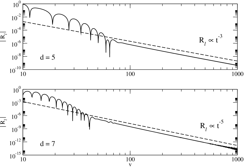
Figure 1: Field decay in the Gauss-Bonnet black holes, for $d=5$ and $d=7$. It is observed a quasinormal mode dominated region. Asymptotically, the field decays as a power-law tail (dashed lines). The parameters in this graph are $\alpha=1$, $\mu=1.0$ and $\ell=0$.

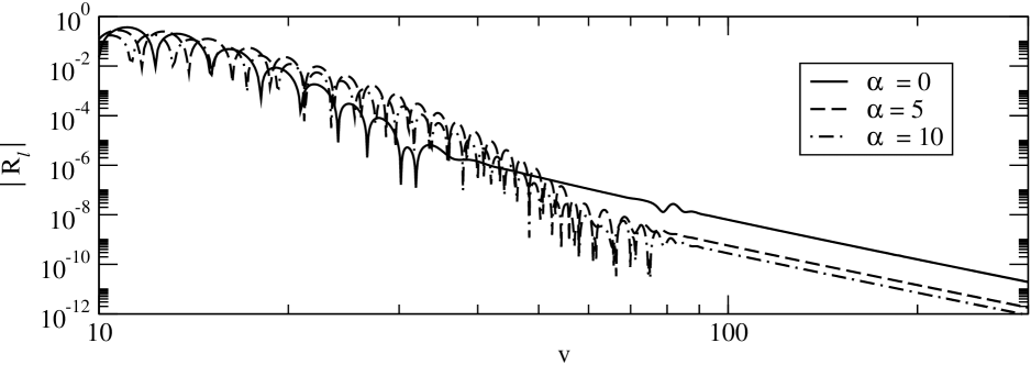
Figure 2: Power-law tails in the Gauss-Bonnet black holes. The estimated power-law are $R_{\ell}\propto t^{-5.076}$, $R_{\ell}\propto t^{-5.082}$ and $R_{\ell}\propto t^{-5.068}$ for $\alpha=0$, $\alpha=5$ and $\alpha=10$ respectively. The predicted power for $\alpha=0$ is $-5$. The parameters in this graph are $d=7$, $\mu=1.0$ and $\ell=0$.

IV.1 Gauss-Bonnet black holes

As seen in a previous work Konoplya05 , the WKB method allows very accurate calculations of the quasinormal modes associated with the field evolution. A complementary analysis can be performed within the time-dependent picture. For this purpose, we use here a characteristic initial value algorithm.

The scenario presented by the WKB calculations is consistent with the results obtained with time evolution approach. From the wave-functions calculated with the characteristic integration routine, it is observed that, after an initial transient phase, the decay is dominated by the quasinormal mode ringing. It is possible to estimate with high precision the oscillatory and exponential decay parameters using a non-linear fitting based in a $\chi^{2}$ analysis. We emphasize that the numerical concordance is excellent, as seen in Tables 1 - 4. The results, as compared between WKB approximation and characteristic integration agree to an accuracy within a few per-cents for $l>n$ case. This small difference must exist, because we compare the data for the fundamental overtones in frequency domain with time domain data where the contribution from all overtones is taken into consideration. Unfortunately the WKB accuracy for $l=n=0$ is not satisfactory what results in large difference between frequency and time domain data for that case.

Strictly speaking, the WKB technique we used here converges only asymptotically. Practically, WKB formula shows good convergence within several few orders after eikonal approximation. Yet, the worse convergence of the WKB method takes place when we deal with the intermediate values of $\alpha\approx 1$. That is why, in this regime, the agreement between the WKB and the characteristic integration results is the worst.

The imaginary part of the frequency does not show too much dependence on $\alpha$, yet slightly decrease when $\alpha$ is increasing. On the other hand, the real part increases with $\alpha$, though not significantly either. This might be showing that a quasinormal mode is much more an effect connected with the local geometry containing the black hole rather than with the global effect of the geometry, namely, the effect of the existence of an event horizon matters much more than a detailed dependence on the parameter $\alpha$. Yet, large enough values of $\alpha$ certainly affect the quasinormal spectrum: the QNMs are proportional to $\alpha$ in the regime of large $\alpha$ Konoplya05 . As $\alpha$ approaches zero, the QNMs go to those of ordinary $d$-dimensional Schwarzschild black hole described by the Tangherlini metric.

However, it does not mean that GB corrections are negligible. On the contrary, according to string theory the Gauss-Bonnet coupling $\alpha$ should be around $1$. Let us compare the results, for instance, for $\ell=2$, $n=0$ QNMs for Schwarzschild and $\alpha=1$ GB black holes for $d=6$: for Schwarzschild we have $\omega=1.5965-0.3967i$ (6th order WKB), for $\alpha=1$ (6th order WKB) we get $\omega=1.69654-0.31929i$ (Note that for this case convergence is good and the 3th order WKB value is not much different $1.67624-0.323698i$). Thus the effect of GB coupling is about $6.3\%$ in real and more then $20\%$ in the imaginary part here. For larger values of $\alpha$ it is certainly larger. We have the same order of difference for other values of $n$ and $\ell$.

Table 1: Values for the quasinormal frequencies for the fundamental mode in the Gauss-Bonnet geometry, obtained from sixth order WKB method and directly from characteristic data, for $d=5$, $\ell=0,1$ and several values of $\alpha$.

d = 5		WKB		Characteristic Integration
$\ell$	$\alpha$	Re($\omega_{0}$)	-Im($\omega_{0}$)	Re($\omega_{0}$)	-Im($\omega_{0}$)
0	0.1	0.389935	0.256159	0.379	0.282
0	0.2	0.396034	0.250548	0.383	0.272
0	0.5	0.429741	0.208293	0.391	0.246
1	0.1	0.720423	0.255506	0.7234	0.250
1	0.2	0.723177	0.252684	0.7284	0.245
1	0.5	0.739205	0.236885	0.7443	0.228

Table 2: Values for the quasinormal frequencies for the fundamental mode in the Gauss-Bonnet geometry, obtained from sixth order WKB method and directly from characteristic data, for $d=6$, $\ell=0,1$ and several values of $\alpha$.

d = 6		WKB		Characteristic Integration
$\ell$	$\alpha$	Re($\omega_{0}$)	-Im($\omega_{0}$)	Re($\omega_{0}$)	-Im($\omega_{0}$)
0	0.1	0.735854	0.402416	0.7109	0.412
0	0.2	0.748053	0.391049	0.7144	0.402
0	0.5	0.83530	0.304837	0.7225	0.375
0	5	0.906661	0.144820	0.9526	0.226
0	10	1.513624	0.456935	1.5182	0.423
0	20	2.961675	0.927128	2.878	0.952
1	0.1	1.139007	0.415034	1.153	0.395
1	0.2	1.136193	0.415706	1.159	0.386
1	0.5	1.158635	0.391339	1.176	0.363
1	5	1.790103	0.258382	1.791	0.253
1	10	3.260415	0.498426	3.253	0.504
1	20	6.437139	0.991374	-	-

Table 3: Values for the quasinormal frequencies for the fundamental mode in the Gauss-Bonnet geometry, obtained from sixth order WKB method and directly from characteristic data, for $d=7$, $\ell=0,1$ and several values of $\alpha$.

d = 7		WKB		Characteristic Integration
$\ell$	$\alpha$	Re($\omega_{0}$)	-Im($\omega_{0}$)	Re($\omega_{0}$)	-Im($\omega_{0}$)
0	0.1	1.11738	0.546056	1.092	0.532
0	0.2	1.13699	0.529543	1.092	0.520
0	0.5	1.29469	0.395111	1.092	0.493
0	5	1.39823	0.574472	1.275	0.351
0	10	1.48053	0.385616	1.515	0.358
0	20	2.00368	0.56458	2.001	0.567
1	0.1	1.54573	0.577608	1.587	0.527
1	0.2	1.53194	0.58701	1.530	0.517
1	0.5	1.56277	0.554551	1.609	0.489
1	5	2.01379	0.308316	1.982	0.337
1	10	2.47824	0.243737	2.475	0.423
1	20	3.39094	0.59452	3.387	0.597

Table 4: Values for the quasinormal frequencies for the fundamental mode in the Gauss-Bonnet geometry, obtained from sixth order WKB method and directly from characteristic data, for $d=8$, $\ell=0,1$ and several values of $\alpha$.

d = 8		WKB		Characteristic Integration
$\ell$	$\alpha$	Re($\omega_{0}$)	-Im($\omega_{0}$)	Re($\omega_{0}$)	-Im($\omega_{0}$)
0	0.1	1.51702	0.694245	1.461	0.676
0	0.2	1.54463	0.673566	1.463	0.658
0	0.5	1.7854	0.488086	1.469	0.616
0	5	1.47941	0.868859	1.647	0.420
0	10	1.800	0.410252	1.838	0.421
0	20	2.15426	0.556954	2.154	0.544
1	0.1	1.93407	0.750046	2.021	0.652
1	0.2	1.90391	0.773947	2.024	0.637
1	0.5	1.94463	0.734591	2.035	0.602
1	5	2.44511	0.455166	2.348	0.434
1	10	2.6644	0.463966	2.670	0.458
1	20	3.2276	0.581024	3.209	0.590

In the time domain the signal has three stages: the initial pulse dependent on the source of perturbations, the quasinormal ringing dominating period, and the power-law tail (see Fig.1). The bigger GB-coupling is, the larger the quasinormal dominated region, i.e. at later times the tails start dominating. As can be seen from Fig.2, the power-law tails do not show dependence on the Gauss-Bonnet coupling $\alpha$ and are the same as for the d-dimensional Schwarzschild black hole in Einstein general relativity, when $d$ is odd. That is, the fields always shows a power-law falloff: for odd $d>3$ the field behaves as

$$R_{\ell}\propto t^{-(2\ell+d-2)}$$ (17)

at late times, where $\ell$ is the multipole number. This behavior is entirely due to $d$ being odd and does not depend on the presence of a black hole Vitor-Tail . It is known, that in Einstein gravity, for even $d>4$, the field decays as Vitor-Tail

$$R_{\ell}\propto t^{-(2\ell+3d-8)}\quad,$$ (18)

and for the latter case there is no contribution from the flat background. This power-law tail is entirely due to the presence of the black hole Vitor-Tail . At the same time, the Gauss-Bonnet black hole metric (3-4) goes to pure Minkowskian metric when the black hole mass equals zero, i.e. in a space-time without a black hole. In other words, empty space-time in Gauss-Bonnet gravity “does not see” the $\alpha$. That is why we do not observe the $\alpha$-dependence of tails in odd space-time dimensions.

Thus, if the Gauss-Bonnet term changes late-time behavior, it must show itself only for even-dimensional space-time. In the numerical procedure developed with the characteristic integration scheme, no tails (power-law or otherwise) were observed in even dimensions Gauss-Bonnet spherical black holes. Yet, it should be pointed out that the integration of the scalar field equation in the GB background is a much more demanding numerical problem than the same integration with the usual Einstein coupling. In the latter case there are auxiliary analytical results, such as explicit expression for the tortoise coordinate function. Therefore, the GB codes are less precise and more time consuming, and eventual tails could be hidden. The possible absence of tails with even $d$ deserves further consideration.

IV.2 Gauss-Bonnet-de Sitter black holes

For the GBdS black holes the quasinormal ringing stage becomes correlated with a new parameter: a positive $\Lambda$-term. When the $\Lambda$-term is growing, both real oscillation frequency and the damping rate are decreasing. Yet, real part of $\omega$ is more sensitive to the changes of $\Lambda$-term.

Qualitatively this resembles the quasinormal oscillations of $d$-dimensional Schwarzschild-de Sitter black hole konoplya03 . In the limit of extremal value of the $\Lambda$-term, i.e. when the cosmological horizon ($r_{c}$) is very close to the event horizon ($r_{+}$), it is possible to generalize the formulas found in Cardoso-03 for four dimensional black hole and in Molina for $d$-dimensional case. Namely, the quasinormal frequencies for the near extreme Gauss-Bonnet asymptotically de Sitter black holes are given by

$$\frac{\omega_{n}}{\kappa_{+}}=\sqrt{\frac{\ell(\ell+d-3)}{r_{+}^{2}}\frac{r_{c}-r_{+}}{2\kappa_{+}}-\frac{1}{4}}-i\left(n+\frac{1}{2}\right)\quad,$$

$$n=0,1,2,\ldots\quad,$$ (19)

where $\kappa_{+}$ (a function of $\alpha$ in this generalized context) is the surface gravity at the event horizon. The above formula is well confirmed numerically: Fig.3 shows a comparison of the values obtained by direct numerical calculation and from Eq. (19). Thus the quasinormal modes are proportional to the surface gravity $\kappa_{+}$, at least for lower overtones. It should be pointed that for the usual Schwarzschild-de Sitter black holes, numerical and analytical investigations SdShigh suggest that the high overtone behavior does not obey the formula (19).

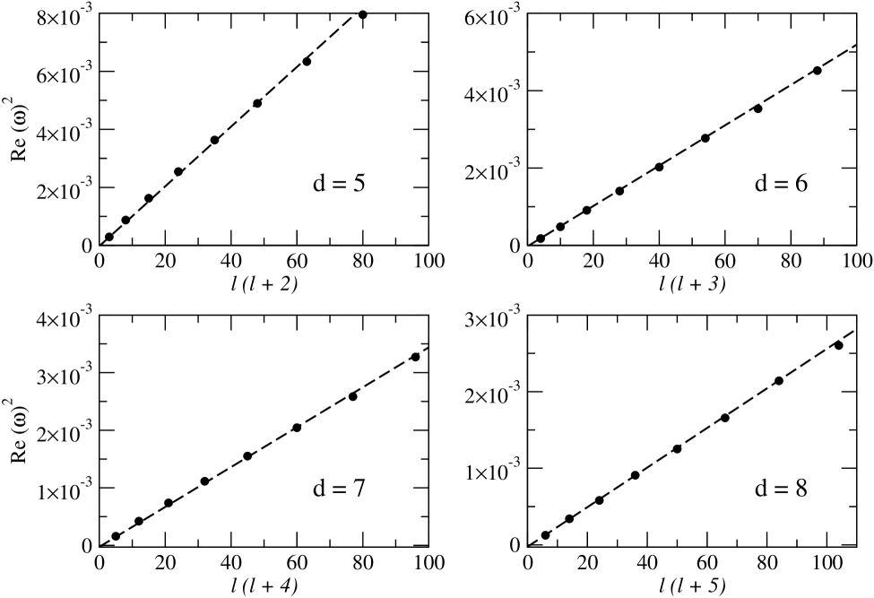
Figure 3: Graph of $\textrm{Re}(\omega)^{2}$ as a function of $\ell(\ell+d-3)$, in the near-extreme limit positive $\Lambda$ limit. The bullets are the values calculated from the time-evolution profiles, and the dashed lines are values obtained from the expression (19). The parameters in this graph are $\kappa_{+}=0.01$, $\alpha=1$, $\mu=1.0$, and the differences between the analytical and numerical results are under 2%.

When the mass parameter $\mu$ is set to zero, we have the case of pure de Sitter spacetime in the Gauss-Bonnet gravity. The metric function (4) then reduces to the following form:

$$h(r)=1+\frac{r^{2}}{2\alpha}-\frac{r^{2}}{2\alpha}\sqrt{1+\frac{8\alpha\Lambda}{(d-1)(d-2)}}\quad.$$ (20)

Repeating the analysis of Abdalla-02 ; natario , we come to the conclusion that quasinormal modes exist only in odd spacetime dimensions and are given by the formula:

$$\omega_{n}=i\left[\frac{1}{2\alpha}\left(1-\sqrt{1+\frac{8\alpha\Lambda}{(d-1)(d-2)}}\right)\right]^{1/2}(2n+\ell)$$

$$n=0,1,2,\ldots\quad.$$ (21)

Note that pure Gauss-Bonnet-de Sitter quasinormal modes are purely imaginary, which corresponds to exponential decaying without oscillations.

It is well-known that the late-time tails of black holes in asymptotically de Sitter space-time for zero multipole and for higher multipoles are qualitatively different. For the zero multipole field ($\ell=0$), the time domain picture is the following: after a transient part, a quasinormal mode dominated region is best observed. Following the quasinormal mode dominated region, a late-time decay region settles. In this latter phase, the wave-functions decay asymptotically to a constant value, as has been the case in the Schwarzschild de Sitter black hole which was studied before Brady-97 ; Brady-99 ; Molina-04 . This is illustrated in Fig.4.

For first and higher multipoles ($\ell>0$) at late times we observe exponential tails in vicinity of GBdS black hole. This is also an expected result, since in Einstein gravity the exponential tails are observed as well in usual de Sitter black holes Brady-97 ; Brady-99 ; Molina-04 . This is illustrated in Fig.5. The dependence of the quasinormal modes on $\Lambda$-term and Gauss-Bonnet coupling can be learnt from Tables X-XII for different space-time dimensionality.

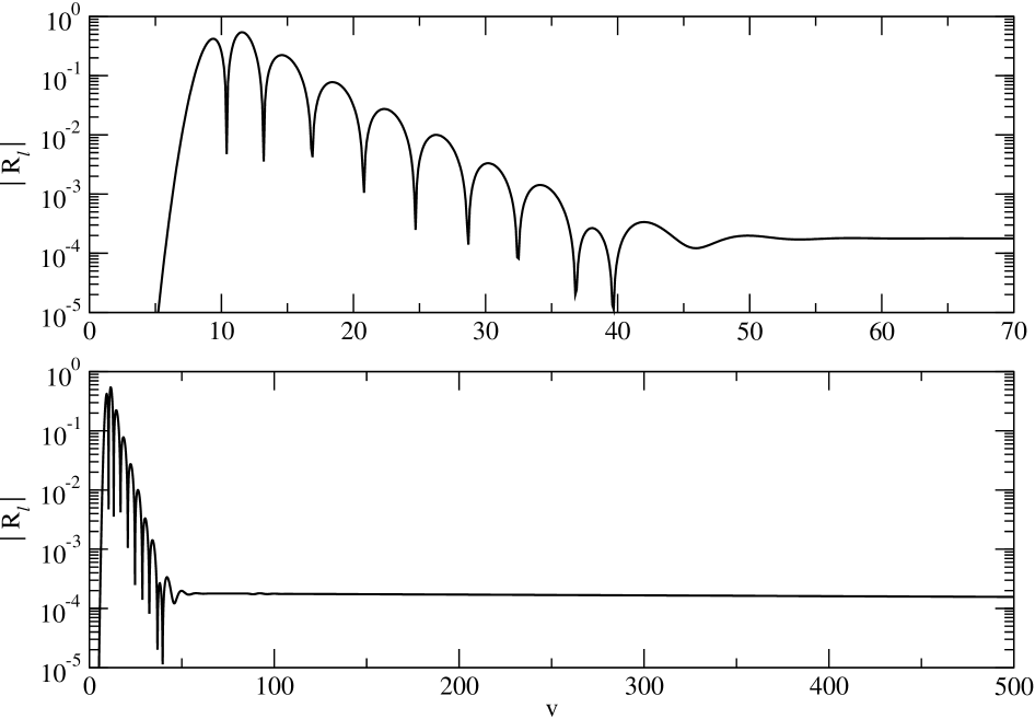
Figure 4: Field decay in the Gauss-Bonnet-de Sitter black holes, with $\ell=0$. A quasinormal mode dominated region is observed (above), and asymptotically the field decays to a constant (below). The fundamental mode, calculated with the WKB method and directly from the characteristic data are $0.8356-0.2935i$ and $0.8011-0.2608i$. The parameters in this graph are $d=6$, $\alpha=3.0$, $\Lambda=0.1$ and $\mu=1.0$.

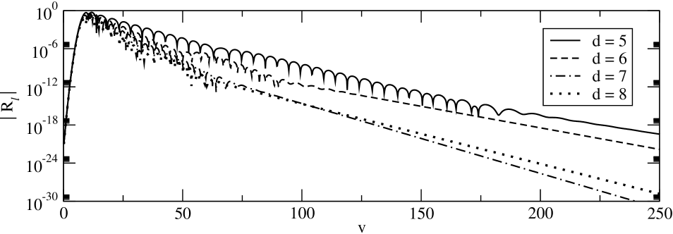
Figure 5: Field decay in the Gauss-Bonnet-de Sitter black holes, for $d=5,6,7,8$. It is observed a quasinormal mode dominated region. Asymptotically, the field decays as an exponential tail. The parameters in this graph are $\alpha=0.1$, $\mu=1.0$ and $\ell=1$.

The numerical simulations developed for Gauss-Bonnet-de Sitter black hole indicate that the massless scalar perturbation in this geometry behave asymptotically as

$$R_{\ell}\approx\exp\left[\ell\left(\kappa_{c}+c^{quad}\kappa_{c}^{2}\right)t\right] t\rightarrow\infty\quad,$$ as

$$d\geq 4\quad\textrm{and}\quad\alpha\geq 0\quad,$$ (22)

where $\kappa_{c}$ is the surface gravity at the cosmological horizon and $c^{quad}$ is an adjustment parameter for the $\kappa_{c}^{2}$ correction. The expression (22) shows that, although the exponential tail in the GBdS background is dependent on the Gauss-Bonnet coupling $\alpha$ (since $\kappa_{c}$ is a function of $\alpha$), the form of the dependence is identical to the null $\alpha$ case. Eq. (22) generalizes the analogous expression found in Molina-04 for the usual Schwarzschild black holes.

Table 5: Values for the quasinormal frequencies for the fundamental mode in the Gauss-Bonnet-de Sitter geometry, obtained from third and sixth order WKB method, for $d=5$, $\ell=0$ and several values of $\alpha$ and $\Lambda$.

d = 5		WKB (3th order)		WKB (6th order)
$\alpha$	$\Lambda$	Re($\omega_{0}$)	-Im($\omega_{0}$)	Re($\omega_{0}$)	-Im($\omega_{0}$)
0.1	1/8	0.30485	0.278407	0.334981	0.26202
0.1	1/2	0.14922	0.217542	0.152444	0.2164
0.1	2/3	0.0677006	0.14792	0.00666957	0.150988
1	1/5	0.301869	0.218752	0.378865	0.159611
1	1	0.112613	0.148749	0.11619	0.145465
1	7/5	0.0240051	0.0683652	0.0242716	0.0709775

Table 6: Values for the quasinormal frequencies for the fundamental mode in the Gauss-Bonnet-de Sitter geometry, obtained from third and sixth order WKB method, for $d=6$, $\ell=0$ and several values of $\alpha$ and $\Lambda$.

d = 6		WKB (3th order)		WKB (6th order)
$\alpha$	$\Lambda$	Re($\omega_{0}$)	-Im($\omega_{0}$)	Re($\omega_{0}$)	-Im($\omega_{0}$)
0.1	1/4	0.580472	0.428367	0.652079	0.411337
0.1	1	0.379931	0.392027	0.401925	0.384688
0.1	2	0.0653851	0.168544	0.0636328	0.173794
1	1/2	0.582293	0.358225	0.736989	0.235326
1	2	0.318697	0.307084	0.331268	0.282461
1	4	0.00390515	0.0487306	0.0574555	0.0529852
10	100	1.5033	0.574511	1.5741	0.599309

Table 7: Values for the quasinormal frequencies for the fundamental mode in the Gauss-Bonnet-de Sitter geometry, obtained from third and sixth order WKB method, for $d=7$, $\ell=0$ and several values of $\alpha$ and $\Lambda$.

d = 7		WKB (3th order)		WKB (6th order)
$\alpha$	$\Lambda$	Re($\omega_{0}$)	-Im($\omega_{0}$)	Re($\omega_{0}$)	-Im($\omega_{0}$)
0.1	1	0.769109	0.556647	0.852395	0.551612
0.1	1	0.561644	0.517639	0.598484	0.511069
0.1	1	0.00963007	0.222564	0.0939457	0.228191
1	1	0.868246	0.48557	1.12603	0.2999562
1	4	0.461426	0.419016	0.483098	0.381285
1	7	0.113334	0.215329	0.111663	0.218394

Table 8: Values for the quasinormal frequencies for the fundamental mode in the Gauss-Bonnet-de Sitter geometry, obtained from third and sixth order WKB method, for $d=8$, $\ell=0$ and several values of $\alpha$ and $\Lambda$.

d = 8		WKB (3th order)		WKB (6th order)
$\alpha$	$\Lambda$	Re($\omega_{0}$)	-Im($\omega_{0}$)	Re($\omega_{0}$)	-Im($\omega_{0}$)
0.1	1	1.1449	0.669364	1.29739	0.695376
0.1	4	0.644892	0.598472	0.682218	0.594199

Table 9: Values for the quasinormal frequencies for the fundamental mode in the Gauss-Bonnet-de Sitter geometry, obtained from third and sixth order WKB method and directly from characteristic data, for $d=5$, $\ell=1$ and several values of $\alpha$ and $\Lambda$.

d = 5		WKB (6th order)		Characteristic Integration
$\alpha$	$\Lambda$	Re($\omega_{0}$)	-Im($\omega_{0}$)	Re($\omega_{0}$)	-Im($\omega_{0}$)
0.1	1/8	0.64317	0.241723	0.6451	0.2382
0.1	1/2	0.379265	0.165101	0.3856	0.1564
0.1	2/3	0.231024	0.103394	0.2247	0.1051
1	1/5	0.698655	0.181854	0.6926	0.1877
1	1	0.365998	0.111668	0.3704	0.1133
1	7/5	0.153506	0.0465747	0.1518	-0.042631

Table 10: Values for the quasinormal frequencies for the fundamental mode in the Gauss-Bonnet-de Sitter geometry, obtained from third and sixth order WKB method and directly from characteristic data, for $d=6$, $\ell=1$ and several values of $\alpha$ and $\Lambda$.

d = 6		WKB (6th order)		Characteristic Integration
$\alpha$	$\Lambda$	Re($\omega_{0}$)	-Im($\omega_{0}$)	Re($\omega_{0}$)	-Im($\omega_{0}$)
0.1	1/4	1.04698	0.39859	1.0574	0.3828
0.1	1	0.74644	0.323514	0.7479	0.3183
0.1	2	0.238066	0.114496	0.2387	0.1212
1	1/2	1.09756	0.301244	1.053	0.2948
1	2	0.6962	0.244326	0.6962	0.2307
1	4	0.0847573	0.0315107	0.08965	0.03323
10	100	3.21004	0.52559	3.1940	0.5360
10	2000	-	-	2.1711	0.4900
10	5000	-	-	0.6228	0.2018

Table 11: Values for the quasinormal frequencies for the fundamental mode in the Gauss-Bonnet-de Sitter geometry, obtained from third and sixth order WKB method and directly from characteristic data, for $d=7$, $\ell=1$, $\alpha=0.1$ and several values of $\Lambda$.

d = 7		WKB (6th order)		Characteristic Integration
$\alpha$	$\Lambda$	Re($\omega_{0}$)	-Im($\omega_{0}$)	Re($\omega_{0}$)	-Im($\omega_{0}$)
0.1	1	1.28621	0.519229	1.304	0.4910
0.1	2	1.00125	0.440876	1.008	0.4306
0.1	4	0.303405	0.153651	0.3091	0.1416
1	1	1.48546	0.411346	1.467	0.3623
1	4	0.899964	0.338928	0.8944	0.3224
1	7	0.361602	0.152214	0.3638	0.1398

Table 12: Values for the quasinormal frequencies for the fundamental mode in the Gauss-Bonnet-de Sitter geometry, obtained from third and sixth order WKB method and directly from characteristic data, for $d=8$, $\ell=1$, $\alpha=0.1$ and several values of $\Lambda$.

d = 8		WKB (6th order)		Characteristic Integration
$\alpha$	$\Lambda$	Re($\omega_{0}$)	-Im($\omega_{0}$)	Re($\omega_{0}$)	-Im($\omega_{0}$)
0.1	1	1.75036	0.697491	1.803	0.6250
0.1	4	1.10954	0.508301	1.103	0.4964

IV.3 Gauss-Bonnet-anti-de Sitter black holes

The quasinormal and late-time behavior of black holes in anti-de Sitter spacetime is significantly different from those in asymptotically de Sitter or flat spacetimes. The key difference is stipulated by the effective potential behavior, which is divergent at spacial infinity. Thus the anti-de Sitter space acts as an effective confining box. Therefore the Dirichlet boundary conditions are natural. These boundary conditions are required also by AdS/CFT correspondence for scalar field perturbations Horowitz00 . Yet, for higher spin perturbations the true boundary conditions may be different moss .

In the usual Schwarzschild-anti-de Sitter black holes, the quasinormal modes govern the decay at all times and thereby no power-law or exponential tails appear Wang-01 ; Wang-04 . We observe a similar behavior the scalar field perturbations in the Gauss-Bonnet-anti-de Sitter black holes.

It is not possible to use WKB method to find the quasinormal modes in Gauss-Bonnet-AdS case because the effective potential is not a potential barrier anymore. The Horowitz-Hubeny method Horowitz00 is not applicable either, because the Taylor expansion of the effective potential has infinite number of terms. That is why we were limited only by time domain analysis, which is free of the above problems. From Fig.6 we see that, indeed, the quasinormal modes are dominating even at sufficiently late times. We also have learnt from Fig.6 that the quasinormal mode dominated region grows, as the multipole index $\ell$ grows.

As is known from Einstein action case, as the radius of the AdS black hole goes to zero, the quasinormal modes of the black hole approach its pure anti-de Sitter values konoplya02 . Repeating the calculations of natario , we find the exact expression for the normal modes in GB gravity:

$$\omega_{n}=\left[\frac{1}{2\alpha}\left(1-\sqrt{1+\frac{8\alpha\Lambda}{(d-1)(d-2)}}\right)\right]^{1/2}(2n+$$

$$\ell+d-1)\quad,$$

$$n=0,1,2,\ldots\quad.$$ (23)

The pure GB-AdS modes, unlike GB-dS modes, exist in any any spacetime dimension.

Table 13: Values for the quasinormal frequencies for the fundamental mode in the Gauss-Bonnet-anti-de Sitter geometry, estimated from the characteristic data, for $d=5$, $\ell=0$, $\mu=1.0$, $\Lambda=-0.1$ and several values of $\alpha$.

$\alpha$	Re($\omega_{0}$)	-Im($\omega_{0}$)
0.1	0.4923	-0.01585
0.1	0.4920	-0.01593
0.5	0.4904	-0.01634
1.0	0.4885	-0.01702
1.5	0.4866	-0.01766

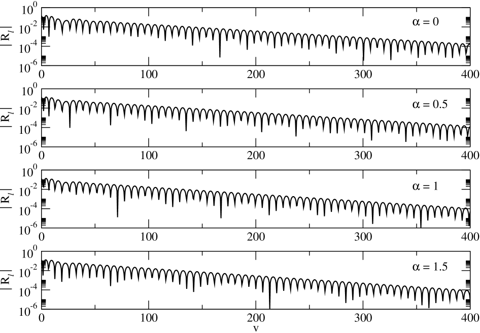
Figure 6: Field decay in the Gauss-Bonnet anti-de Sitter black holes, for several values of the Gauss-Bonnet coupling. It is observed a quasinormal mode dominated region. Asymptotically, the field decays in quasinormal modes. The parameters in this graph are $d=5$, $\mu=1.0$ $\Lambda=-0.1$ and $\ell=0$.

V Conclusions

We have considered here frequency and time domain description of evolution of scalar field perturbations in the exterior of black holes in Gauss-Bonnet theory of gravity, generally with a $\Lambda$-term. The quasinormal behavior even though being corrected by a new parameter, Gauss-Bonnet coupling $\alpha$, are qualitatively dependent mainly on the $\Lambda$-term and black hole parameters such as mass $\mu$ and multipole number $\ell$. The late-time tails for asymptotically flat Gauss-Bonnet black holes, do not depend on the Gauss-Bonnet coupling in odd space-time dimensions, and therefore are the same as those for d-dimensional Schwarzschild black hole in Einstein gravity. Moreover, in the case of Gauss-Bonnet-de Sitter black holes, the late-time tails, though dependent on $\alpha$, yet, rather trivially, i.e. only through dependence of the surface gravity at the cosmological radius on $\alpha$. Thus, the Gauss-Bonnet coupling shows itself “minimally” in late-time behavior. The most interesting problem which remains unsolved is, to find late time tails for even dimensions, and thereby, to know whether the power-law tails depend upon the Gauss-Bonnet term. At the same time, we have shown that corrections to the quasinormal frequencies due to GB-term are not negligible: they may reach $20\%$ for string theory predicted values of $\alpha\approx 1$.

Even though our analysis can easily be extended to the massive scalar field, we were limited here by the massless case. We expect that the influence of the massive term upon the QNMs will be similar to that found in konoplyaPLB , i.e. the lower overtones should be corrected by the field mass, infinitely high overtone asymptotic will be unchanged no matter the value of the massive term. Also we did not consider the high overtone behavior of the GB black holes. Generally, the high overtone asymptotics must be studied by totally different methods high-n and deserves separate investigation.

- (1) L. Randall and R. Sundrum, Phys. Rev. Lett. 83 3370, 4690 (1999).
- (2) D. G. Boulware and S. Deser, Phys. Rev. Lett. 55, 2656 (1985).
- (3) J. Wheeler, Nucl. Phys. B268, 737 (1986).
- (4) D. Lovelock, J. Math. Phys. 12, 498 (1971).
- (5) J. Crisostomo, R. Troncoso and J. Zanelli, Phys. Rev. D 62, 084013 (2000).
- (6) Elcio Abdalla and L. Alejandro Correa-Borbonet, Phys. Rev. D 65, 124011 (2002).
- (7) V. S. Rychkov, Phys. Rev. D 70, 044003 (2004).
- (8) G. Duffy, C. Harris, P. Kanti, E. Winstanley, hep-th/0507274 (2005).
- (9) K. D. Kokkotas and B. G. Schmidt, Living Rev. Relativity 2, 2 (1999).
- (10) S. Nojiri, S. D. Odintsov, J. of High Energy Phys. 0007, 049 (2000).
- (11) G. T. Horowitz and V. E. Hubeny, Phys. Rev. D 62, 024027 (2000); A. Nunez, A. O. Starinets, Phys. Rev. D 67, 124013 (2003).
- (12) R. Konoplya, Phys. Rev. D 71, 024038 (2005) [hep-th/0410057].
- (13) B. F. Schutz and C. M. Will, Astrophys. J. 291, L33 (1985); S. Iyer and C. M. Will, Phys. Rev. D 35, 3621 (1987); R. A. Konoplya, Phys. Rev. D 68, 024018 (2003) [gr-qc/0303052].
- (14) G. Dotti, R. J. Gleiser, gr-qc/0503117.
- (15) Rodrigo Olea, J. of High Energy Phys. 0506, 023 (2005).
- (16) C. Gundlach, R. Price and J. Pullin, Phys. Rev. D 49, 883 (1994).
- (17) R. Price, Phys. Rev. D 5, 2419 (1972).
- (18) P. R. Brady, C. M. Chambers, W. Krivan and P. Laguna, Phys. Rev. D 55, 7538 (1997).
- (19) P. R. Brady, C. M. Chambers, W. G. Laarakkers and E. Poisson, Phys. Rev. D 60, 064003 (1999).
- (20) I.G. Moss and J.P. Norman, Class. Quant. Grav. 19, 2323 (2002)
- (21) B. Wang, C. Molina and E. Abdalla, Phys. Rev. D 63, 084001 (2001).
- (22) Bin Wang, Chi-Yong Lin, C. Molina, Phys. Rev. D 70, 064025 (2004).
- (23) E. Berti, K. D. Kokkotas, Phys. Rev. D 71, 124008 (2005); R. A. Konoplya, Phys. Rev. D 66, 084007 (2002) [gr-qc/0207028]; S. Fernando, Gen. Rel. Grav. 37, 585 (2005); R. A. Konoplya, E. Abdalla, Phys. Rev. D 71, 084015 (2005) [hep-th/0503029]; R. A. Konoplya, C. Molina, Phys. Rev. D 71, 124009 (2005) [gr-qc/0504139]; H. Nomura, T. Tamaki, Phys. Rev. D 71, 124033 (2005).
- (24) V. Cardoso, S. Yoshida, O.J.C. Dias, J. P.S. Lemos, Phys. Rev.D 68, 061503 (2003).
- (25) R. A. Konoplya, Phys. Rev. D 68, 124017 (2003) [hep-th/0309030].
- (26) V. Cardoso and J. P. S. Lemos, Phys. Rev. D 67 084020 (2003).
- (27) C. Molina, Phys.Rev. D 69, 104013 (2004).
- (28) S. Yoshida and T. Futamase, PRD 69, 064025 (2004); V. Cardoso, J. Natario, R. Schiappa, J. Math. Phys. 45 4698 (2004); R. A. Konoplya and A. Zhidenko, J. of High Energy Phys. 037, 06 (2004) [hep-th/0402080].
- (29) E. Abdalla, K. H. C. Castello-Branco, A. Lima-Santos, Phys. Rev. D 66, 104018 (2002).
- (30) J. Natario, R. Schiappa, hep-th/0411267 (to be published in Adv. Theor. Math. Phys.).
- (31) C. Molina, D. Giugno, E. Abdalla, A. Saa, Phys.Rev. D 69, 104013 (2004).
- (32) R. A. Konoplya, Phys. Rev. D 66, 044009 (2002) [hep-th/0205142].
- (33) R. A. Konoplya, Phys. Lett. B 550, 117 (2002) [gr-qc/0210105]; R. A. Konoplya, A. V. Zhidenko, Phys. Lett. B 609, 377 (2005) [gr-qc/0411059].
- (34) H-P Nollert, Phys. Rev. D 47, 5253 (1993); V. Cardoso, R. Konoplya, J. P.S. Lemos, Phys. Rev. D 68, 044024 (2003) [gr-qc/0305037]; L. Motl and A. Neitzke, Adv. Theor. Math. Phys. 7, 307 (2003).
- (35) E. Berti, M. Cavaglia and L. Gualtieri, Phys. Rev. D69, 124011 (2004); H. Yoshino, T. Shiromizu and M. Shibata, gr-qc/0508063.
- (36) V.Cardoso, J.Lemos, S. Yoshida, Phys. Rev. D 69, 044004 (2004).