TIFR/TH/05-25

hep-th/0507096

Non-Supersymmetric Attractors

Kevin Goldstein, Norihiro Iizuka, Rudra P. Jena and Sandip P. Trivedi

Tata Institute of Fundamental Research

Homi Bhabha Road, Mumbai, 400 005, INDIA

kevin, iizuka, rpjena, sandip@theory.tifr.res.in

Abstract

We consider theories with gravity, gauge fields and scalars in four-dimensional asymptotically flat space-time. By studying the equations of motion directly we show that the attractor mechanism can work for non-supersymmetric extremal black holes. Two conditions are sufficient for this, they are conveniently stated in terms of an effective potential involving the scalars and the charges carried by the black hole. Our analysis applies to black holes in theories with ${\cal N}\leqslant 1$ supersymmetry, as well as non-supersymmetric black holes in theories with ${\cal N}=2$ supersymmetry. Similar results are also obtained for extremal black holes in asymptotically Anti-de Sitter space and in higher dimensions.

1 Introduction

Black holes in ${\cal N}=2$ supersymmetric theories are known to exhibit a fascinating phenomenon called the the attractor mechanism. There is a family of black hole solutions in these theories which are spherically symmetric, extremal black holes, with double-zero horizons . In these solutions several moduli fields are drawn to fixed values at the horizon of the black hole regardless of the values they take at asymptotic infinity. The fixed values are determined entirely by the charges carried by the black hole. This phenomenon was first discussed by [1] and has been studied quite extensively since then [2, 3, 4, 5, 6, 7, 8, 9, 10]. It has gained considerable attention recently due to the conjecture of [11] and related developments [12, 13, 14, 15].

So far the attractor phenomenon has been studied almost exclusively in the context of BPS black holes in the ${\cal N}=2$ theories. The aim of this paper is to examine if it is more general and can happen for non-supersymmetric black holes as well. These black holes might be solutions in theories which have no supersymmetry or might be non-supersymmetric solutions in ${\cal N}\geqslant 1$ supersymmetric theories.

There are two motivations for this investigation. First, a non-supersymmetric attractor mechanism might help in the study of non-supersymmetric black holes, especially their entropy. Second, given interesting parallels between flux compactifications and the attractor mechanisms, a non-supersymmetric attractor phenomenon might lead to useful lessons for non-supersymmetric flux compactifications. For example, it could help in finding dual descriptions of such compactifications. This might help to single out vacua with a small cosmological constant. Or it might suggest ways to weight vacua with small cosmological constants preferentially while summing over all of them . These lessons would be helpful in light of the vast number of vacua that have been recently uncovered in string theory [16].

An intuitive argument for the attractor mechanism is as follows. One expects that the total number of microstates corresponding to an extremal black hole is determined by the quantised charges it carries, and therefore does not vary continuously. If the counting of microstates agrees with the Bekenstein-Hawking entropy, that is the horizon area, it too should be determined by the charges alone. This suggests that the moduli fields which determine the horizon area take fixed values at the horizon, and these fixed values depend only on the charges, independent of the asymptotic values for the moduli. While this argument is only suggestive what is notable for the present discussion is that it does not rely on supersymmetry. This provides further motivation to search for a non-supersymmetric version of the attractor mechanism.

The theories we consider in this paper consist of gravity, gauge fields and scalar fields. The scalars determine the gauge couplings and there by couple to the gauge fields. It is important that the scalars do not have a potential of their own that gives them in particular a mass. Such a potential would mean that the scalars are no longer moduli.

We first study black holes in asymptotically flat four dimensions. Our main result is to show that the attractor mechanism works quite generally in such theories provided two conditions are met. These conditions are succinctly stated in terms of an “effective potential” $V_{eff}$ for the scalar fields, $\phi_{i}$. The effective potential is proportional to the energy density in the electromagnetic field and arises after solving for the gauge fields in terms of the charges carried by the black hole, as we explain in more detail below. The two conditions that need to be met are the following. First, as a function of the moduli fields $V_{eff}$ must have a critical point, $\partial_{i}V_{eff}(\phi_{i0})=0$. And second, the matrix of second derivatives of the effective potential at the critical point, $\partial_{ij}V_{eff}(\phi_{i0})$, must be have only positive eigenvalues. The resulting attractor values for the moduli are the critical values, $\phi_{i0}$. And the entropy of the black hole is proportional to $V(\phi_{i0})$, and is thus independent of the asymptotic values for the moduli. It is worth noting that the two conditions stated above are met by BPS black hole attractors in an ${\cal N}=2$ theory.

The analysis for BPS attractors simplifies greatly due to the use of the first order equations of motion. In the non-supersymmetric context one has to work with the second order equations directly and this complicates the analysis. We find evidence for the attractor mechanism in three different ways. First, we analyse the equations using perturbation theory. The starting point is a black hole solution, where the asymptotic values for the moduli equal their critical values. This gives rise to an extremal Reissner Nordstrom black hole. By varying the asymptotic values a little at infinity one can now study the resulting equations in perturbation theory. Even though the equations are second order, in perturbation theory they are linear, and this makes them tractable. The analysis can be carried out quite generally for any effective potential for the scalars and shows that the two conditions stated above are sufficient for the attractor phenomenon to hold.

Second, we carry out numerical analysis. This requires a specific form of the effective potential, but allows us to go beyond the perturbative regime. The numerical analysis corroborates the perturbation theory results mentioned above. In simple cases we have explored so far, we have found evidence for a only single basin of attraction, although multiple basins must exist in general as is already known from the SUSY cases.

Finally, in some special cases, we solve the equations of motion exactly by mapping them a solvable Toda system. This allows us to study the black hole solutions in these special cases in some depth. Once again, in all the cases we have studied, we can establish the attractor phenomenon.

It is straightforward to generalise these results to other settings. We find that the attractor phenomenon continues to hold in Anti-de Sitter space (AdS) and also in higher dimensions, as long as the two conditions mentioned above are valid for a suitable defined effective potential. There is also possibly an attractor mechanism in de Sitter space (dS), but in the simplest of situations analysed here some additional caveats have to be introduced to deal with infrared divergences in the far past (or future) of dS space.

This paper is structured as follows. Black holes in asymptotically flat four dimensional space are analysed first, in sections 2,3,4. The discussion is extended to asymptotically flat space-times of higher dimension in section 5. Asymptotically AdS space is discussed next in section 6.

As was mentioned above our analysis in the asymptotically flat and AdS cases is based on theories which have no potential for the scalars so that their values can vary at infinity. Some comments on this are contained in Section 7. With ${\cal N}\geqslant 1$ SUSY such theories can arise, with the required couplings between scalars and gauge fields, and are at least technically natural. In the absence of supersymmetry there is no natural way to arrange this and our study is more in the nature of a mathematical investigation. We follow in section 8, with some comments on the attractor phenomenon in dS. Finally, in section 9 we show that non-extremal black holes do not have an attractor mechanism. Thus, the double-zero nature of the horizon is essential to draw the moduli to fixed values.

Several important intermediate steps in the analysis are discussed in appendices A-D.

Some important questions are left for the future. First, we have not analysed the stability of these black hole solutions. It is unlikely that there are any instabilities at least in the S-wave sector. We do not attempt a general analysis of small fluctuations here. Second, in this paper we have not analysed string theory situations where such non-supersymmetric black holes can arise [17]. This could include both critical and non-critical string theory. In case of ${\cal N}=1$ supersymmetry it would be interesting to explore if there is partial restoration of supersymmetry at the horizon. Given the rotational invariance of the solutions one can see that no supersymmetry is preserved in-between asymptotic infinity and the horizon in this case.

Let us also briefly comment on some of the literature of especial relevance. The importance of the effective potential, $V_{eff}$, for ${\cal N}=2$ black holes was emphasised in [9]. Some comments pertaining to the non-supersymmetric case can be found for example in [7]. A similar analysis using an effective one dimensional theory, and the Gauss-Bonett term, was carried out in [18]. Finally, while the thrust of the analysis is different, our results are quite closely related to those in [19] which appeared while this paper was in preparation (see also [20] for the 3-dimensional case). In [19] the entropy (including higher derivative corrections) is obtained from the gauge field Lagrangian after carrying out a Legendre transformation with respect to the electric parameters. This is similar to our result which is based on $V_{eff}$. As was mentioned above, $V_{eff}$, is proportional to the electro-magnetic energy density i.e., the Hamiltonian density of the electro-magnetic fields, and is derived from the Lagrangian by doing a canonical transformation with respect to the gauge fields. For an action with only two-derivative terms, our results and those in [19] agree [21].

2 Attractor in Four-Dimensional Asymptotically Flat Space

2.1 Equations of Motion

In this section we consider gravity in four dimensions with $U(1)$ gauge fields and scalars. The scalars are coupled to gauge fields with dilaton-like couplings. It is important for the discussion below that the scalars do not have a potential so that there is a moduli space obtained by varying their values.

The action we start with has the form,

$$S=\frac{1}{\kappa^{2}}\int d^{4}x\sqrt{-G}(R-2(\partial\phi_{i})^{2}-f_{ab}(\phi_{i})F^{a}_{\mu\nu}F^{b\ \mu\nu})$$ (1)

Here the index $i$ denotes the different scalars and $a,b$ the different gauge fields and $F^{a}_{\mu\nu}$ stands for the field strength of the gauge field. $f_{ab}(\phi_{i})$ determines the gauge couplings, we can take it to be symmetric in $a,b$ without loss of generality.

The Lagrangian is

$${\mathcal{L}}=(R-2(\partial\phi_{i})^{2}-f_{ab}(\phi_{i})F^{a}_{\mu\nu}F^{b\ \mu\nu})$$ (2)

Varying the metric gives ,

$$R_{\mu\nu}-2\partial_{\mu}\phi_{i}\partial_{\nu}\phi_{i}=2f_{ab}(\phi_{i})F^{a}_{\phantom{a}\mu\lambda}F^{b\phantom{\nu}\lambda}_{\phantom{b}\nu}+\frac{1}{2}G_{\mu\nu}\mathcal{L}$$ (3)

The trace of the above equation implies

$$R-2(\partial\phi_{i})^{2}=0$$ (4)

The equations of motion corresponding to the metric, dilaton and the gauge fields are then given by,

$$R_{\mu\nu}-2\partial_{\mu}\phi_{i}\partial_{\nu}\phi_{i} = f_{ab}(\phi_{i})\left(2F^{a}_{\phantom{a}\mu\lambda}F^{b\phantom{\nu}\lambda}_{\phantom{b}\nu}-{\textstyle\frac{1}{2}}G_{\mu\nu}F^{a}_{\phantom{a}\kappa\lambda}F^{b\kappa\lambda}\right)$$ (5)

$$\frac{1}{\sqrt{-G}}\partial_{\mu}(\sqrt{-G}\partial^{\mu}\phi_{i}) = {1\over 4}\partial_{i}(f_{ab})F^{a}_{\phantom{a}\mu\nu}F^{b\mu\nu}$$ (6)

$$\partial_{\mu}(\sqrt{-G}f_{ab}(\phi_{i})F^{b\mu\nu}) = 0.$$

The Bianchi identity for the gauge field is,

$$\partial_{\mu}F_{\nu\rho}+\partial_{\nu}F_{\rho\mu}+\partial_{\rho}F_{\mu\nu}=0.$$ (7)

We now assume all quantities to be function of $r$. To begin, let us also consider the case where the gauge fields have only magnetic charge, generalisations to both electrically and magnetically charged cases will be discussed shortly. The metric and gauge fields can then be written as,

$$ds^{2} = -a(r)^{2}dt^{2}+a(r)^{-2}dr^{2}+b(r)^{2}d\Omega^{2}$$ (8)

$$F^{a} = Q_{m}^{a}sin\theta d\theta\wedge d\phi$$ (9)

Using the equations of motion we then get,

$$R_{tt} = \frac{a^{2}}{b^{4}}V_{eff}(\phi_{i})$$ (10)

$$R_{\theta\theta} = \frac{1}{b^{2}}V_{eff}(\phi_{i})$$ (11)

where,

$$V_{eff}(\phi_{i})\equiv f_{ab}(\phi_{i})Q_{m}^{a}Q_{m}^{b}.$$ (12)

This function, $V_{eff}$, will play an important role in the subsequent discussion. We see from eq.(10) that up to an overall factor it is the energy density in the electromagnetic field. Note that $V_{eff}(\phi_{i})$ is actually a function of both the scalars and the charges carried by the black hole.

The relation, $R_{tt}=\frac{a^{2}}{b^{2}}R_{\theta\theta}$, after substituting the metric ansatz implies that,

$$(a^{2}(r)b^{2}(r))^{{}^{\prime\prime}}=2.$$ (13)

The $R_{rr}-{G^{tt}\over G^{rr}}R_{tt}$ component of the Einstein equation gives

$$\frac{b^{{}^{\prime\prime}}}{b}=-(\partial_{r}\phi)^{2}.$$ (14)

Also the $R_{rr}$ component itself yields a first order “energy” constraint,

$$-1+a^{2}b^{{}^{\prime}2}+\frac{a^{2^{\prime}}b^{2^{\prime}}}{2}=\frac{-1}{b^{2}}(V_{eff}(\phi_{i}))+a^{2}b^{2}(\phi^{\prime})^{2}$$ (15)

Finally, the equation of motion for the scalar $\phi_{i}$ takes the form,

$$\partial_{r}(a^{2}b^{2}\partial_{r}\phi_{i})=\frac{\partial_{i}V_{eff}}{2b^{2}}.$$ (16)

We see that $V_{eff}(\phi_{i})$ plays the role of an “effective potential ” for the scalar fields.

Let us now comment on the case of both electric and magnetic charges. In this case one should also include “axion” type couplings and the action takes the form,

$$S=\frac{1}{\kappa^{2}}\int d^{4}x\sqrt{-G}(R-2(\partial\phi_{i})^{2}-f_{ab}(\phi_{i})F^{a}_{\phantom{a}\mu\nu}F^{b\,\mu\nu}-{\textstyle{1\over 2}}{\tilde{f}}_{ab}(\phi_{i})F^{a}_{\phantom{a}\mu\nu}F^{b}_{\phantom{b}\rho\sigma}\epsilon^{\mu\nu\rho\sigma}).$$ (17)

We note that ${\tilde{f}}_{ab}(\phi_{i})$ is a function independent of $f_{ab}(\phi_{i})$, it can also be taken to be symmetric in $a,b$ without loss of generality.

The equation of motion for the metric which follows from this action is unchanged from eq.(5). While the equations of motion for the dilaton and the gauge field now take the form,

$$\frac{1}{\sqrt{-G}}\partial_{\mu}(\sqrt{-G}\partial^{\mu}\phi_{i})=\textstyle{1\over 4}\partial_{i}(f_{ab})F^{a}_{\phantom{a}\mu\nu}F^{b\,\mu\nu}+\textstyle{1\over 8}\partial_{i}({\tilde{f}}_{ab})F^{a}_{\phantom{a}\mu\nu}F^{b}_{\phantom{b}\rho\sigma}\epsilon^{\mu\nu\rho\sigma}$$ (18)

$$\partial_{\mu}\left(\sqrt{-G}\left(f_{ab}(\phi_{i})F^{b\,\mu\nu}+\textstyle{1\over 2}{\tilde{f}}_{ab}F^{b}_{\phantom{b}\rho\sigma}\epsilon^{\mu\nu\rho\sigma}\right)\right)=0.$$ (19)

With both electric and magnetic charges the gauge fields take the form,

$$F^{a}=f^{ab}(\phi_{i})(Q_{eb}-{\tilde{f}}_{bc}Q^{c}_{m}){1\over b^{2}}dt\wedge dr+Q_{m}^{a}sin\theta d\theta\wedge d\phi,$$ (20)

where $Q_{m}^{a},Q_{ea}$ are constants that determine the magnetic and electric charges carried by the gauge field $F^{a}$, and $f^{ab}$ is the inverse of $f_{ab}$ . It is easy to see that this solves the Bianchi identity eq.(7), and the equation of motion for the gauge fields eq.(19).

A little straightforward algebra shows that the Einstein equations for the metric and the equations of motion for the scalars take the same form as before, eq.(13, 14, 15, 16), with $V_{eff}$ now being given by,

$$V_{eff}(\phi_{i})=f^{ab}(Q_{ea}-{\tilde{f}}_{ac}Q^{c}_{m})(Q_{eb}-{\tilde{f}}_{bd}Q^{d}_{m})+f_{ab}Q^{a}_{m}Q^{b}_{m}.$$ (21)

As was already noted in the special case of only magnetic charges, $V_{eff}$ is proportional to the energy density in the electromagnetic field and therefore has an immediate physical significance. It is invariant under duality transformations which transform the electric and magnetic fields to one-another.

Our discussion below will use (13, 14, 15, 16) and will apply to the general case of a black hole carrying both electric and magnetic charges.

It is also worth mentioning that the equations of motion, eq.(13, 14, 16) above can be derived from a one-dimensional action,

$$S=\frac{2}{\kappa^{2}}\int dr\left((a^{2}b)^{{}^{\prime}}b^{{}^{\prime}}-a^{2}b^{2}(\phi^{\prime})^{2}-\frac{V_{eff}(\phi_{i})}{b^{2}}\right).$$ (22)

The constraint, eq.(15) must be imposed in addition.

One final comment before we proceed. The eq.(17) can be further generalised to include non-trivial kinetic energy terms for the scalars of the form,

$$\int d^{4}x\sqrt{-G}\left(-g_{ij}(\phi_{k})\partial\phi^{i}\partial\phi^{j}\right).$$ (23)

The resulting equations are easily determined from the discussion above by now contracting the scalar derivative terms with the metric $g_{ij}$. The two conditions we obtain in the next section for the existence of an attractor are not altered due to these more general kinetic energy terms.

2.2 Conditions for an Attractor

We can now state the two conditions which are sufficient for the existence of an attractor. First, the charges should be such that the resulting effective potential, $V_{eff}$, given by eq.(21), has a critical point. We denote the critical values for the scalars as $\phi_{i}=\phi_{i0}$. So that,

$$\partial_{i}V_{eff}(\phi_{i0})=0$$ (24)

Second, the matrix of second derivatives of the potential at the critical point,

$$M_{ij}={1\over 2}\partial_{i}\partial_{j}V_{eff}(\phi_{i0})$$ (25)

should have positive eigenvalues. Schematically we write,

$$M_{ij}>0$$ (26)

Once these two conditions hold, we show below that the attractor phenomenon results. The attractor values for the scalars are $\phi_{i}=\phi_{i0}$.

The resulting horizon radius is given by,

$$b_{H}^{2}=V_{eff}(\phi_{i0})$$ (27)

and the entropy is

$$S_{BH}={1\over 4}A=\pi b_{H}^{2}.$$ (28)

There is one special solution which plays an important role in the discussion below. From eq.(16) we see that one can consistently set $\phi_{i}=\phi_{i0}$ for all values of $r$. The resulting solution is an extremal Reissner Nordstrom (ERN) Black hole. It has a double-zero horizon. In this solution $\partial_{r}\phi_{i}=0$, and $a,b$ are

$$a_{0}(r)=\left(1-\frac{r_{H}}{r}\right),\,\,\ b_{0}(r)=r$$ (29)

where $r_{H}$ is the horizon radius. We see that $a_{0}^{2},(a_{0}^{2})^{\prime}$ vanish at the horizon while $b_{0},b_{0}^{\prime}$ are finite there. From eq.(15) it follows then that the horizon radius $b_{H}$ is indeed given by

$$r_{H}^{2}=b_{H}^{2}=V_{eff}(\phi_{i0}),$$ (30)

and the black hole entropy is eq.(28).

If the scalar fields take values at asymptotic infinity which are small deviations from their attractor values we show below that a double-zero horizon black hole solution continues to exist. In this solution the scalars take the attractor values at the horizon, and $a^{2},(a^{2})^{\prime}$ vanish while $b,b^{\prime}$ continue to be finite there. From eq.(15) it then follows that for this whole family of solutions the entropy is given by eq.(28) and in particular is independent of the asymptotic values of the scalars.

For simple potentials $V_{eff}$ we find only one critical point. In more complicated cases there can be multiple critical points which are attractors, each of these has a basin of attraction.

One comment is worth making before moving on. A simple example of a system which exhibits the attractor behaviour consists of one scalar field $\phi$ coupled to two gauge fields with field strengths, $F^{a},a=1,2$. The scalar couples to the gauge fields with dilaton-like couplings,

$$f_{ab}(\phi)=e^{\alpha_{a}\phi}\delta_{ab}.$$ (31)

If only magnetic charges are turned on,

$$V_{eff}=e^{\alpha_{1}\phi}(Q_{1})^{2}+e^{\alpha_{2}\phi}(Q_{2})^{2}.$$ (32)

(We have suppressed the subscript “$m$” on the charges). For a critical point to exist $\alpha_{1}$ and $\alpha_{2}$ must have opposite sign. The resulting critical value of $\phi$ is given by,

$$e^{\phi_{0}}=\left(-\frac{\alpha_{2}(Q_{2})^{2}}{\alpha_{1}(Q_{1})^{2}}\right)^{\frac{1}{\alpha_{1}-\alpha_{2}}}$$ (33)

The second derivative, eq.(25) now is given by

$${\partial^{2}V_{eff}\over\partial\phi^{2}}=-2\alpha^{1}\alpha^{2}$$ (34)

and is positive if $\alpha_{1},\alpha_{2}$ have opposite sign.

This example will be useful for studying the behaviour of perturbation theory to higher orders and in the subsequent numerical analysis.

As we will discuss further in section 7, a Lagrangian with dilaton-like couplings of the type in eq.(31), and additional axionic terms ( which can be consistently set to zero if only magnetic charges are turned on), can always be embedded in a theory with ${\cal N}=1$ supersymmetry. But for generic values of $\alpha$ we do not expect to be able to embed it in an ${\cal N}=2$ theory. The resulting extremal black hole, for generic $\alpha$, will also then not be a BPS state.

2.3 Comparison with the ${\cal N}=2$ Case

It is useful to compare the discussion above with the special case of a BPS black hole in an ${\cal N}=2$ theory. The role of the effective potential, $V_{eff}$ for this case was emphasised by Denef, [9]. It can be expressed in terms of a superpotential $W$ and a Kahler potential $K$ as follows:

$$V_{eff}=e^{K}[K^{i\bar{j}}D_{i}W(D_{j}W)^{*}+|W|^{2}],$$ (35)

where $D_{i}W\equiv\partial_{i}W+\partial_{i}KW$. The attractor equations take the form,

$$D_{i}W=0$$ (36)

And the resulting entropy is given by

$$S_{BH}=\pi|W|^{2}e^{K}.$$ (37)

with the superpotential evaluated at the attractor values.

It is easy to see that if eq.(36) is met then the potential is also at a critical point, $\partial_{i}V_{eff}=0$. A little more work also shows that all eigenvalues of the second derivative matrix, eq.(25) are also positive in this case. Thus the BPS attractor meets the two conditions mentioned above. We also note that from eq.(35) the value of $V_{eff}$ at the attractor point is $V_{eff}=e^{K}|W|^{2}$. The resulting black hole entropy eq.(27, 28) then agrees with eq.(37).

We now turn to a more detailed analysis of the attractor conditions below.

2.4 Perturbative Analysis

2.4.1 A Summary

The essential idea in the perturbative analysis is to start with the extremal RN black hole solution described above, obtained by setting the asymptotic values of the scalars equal to their critical values, and then examine what happens when the scalars take values at asymptotic infinity which are somewhat different from their attractor values, $\phi_{i}=\phi_{i0}$.

We first study the scalar field equations to first order in the perturbation, in the ERN geometry without including backreaction. Let $\phi_{i}$ be a eigenmode of the second derivative matrix eq.(25) . Then denoting, $\delta\phi_{i}\equiv\phi_{i}-\phi_{i0}$, neglecting the gravitational backreaction, and working to first order in $\delta\phi_{i}$, we find that eq.(16) takes the form,

$$\partial_{r}\left((r-r_{H})^{2}\partial_{r}(\delta\phi_{i})\right)={\beta_{i}^{2}\delta\phi_{i}\over r^{2}},$$ (38)

where $\beta_{i}^{2}$ is the relevant eigenvalue of ${1\over 2}\partial_{i}\partial_{j}V(\phi_{i0})$. In the vicinity of the horizon, we can replace the factor $1/r^{2}$ on the r.h.s by a constant and as we will see below, eq.(38), has one solution that is well behaved and vanishes at the horizon provided $\beta_{i}^{2}\geqslant 0$. Asymptotically, as $r\rightarrow\infty$, the effects of the gauge fields die away and eq.(38) reduces to that of a free field in flat space. This has two expected solutions, $\delta\phi_{i}\sim constant$, and $\delta\phi_{i}\sim 1/r$, both of which are well behaved. It is also easy to see that the second order differential equation is regular at all points in between the horizon and infinity. So once we choose the non-singular solution in the vicinity of the horizon it can be continued to infinity without blowing up.

Next, we include the gravitational backreaction. The first order perturbations in the scalars source a second order change in the metric. The resulting equations for metric perturbations are regular between the horizon and infinity and the analysis near the horizon and at infinity shows that a double-zero horizon black hole solution continues to exist which is asymptotically flat after including the perturbations.

In short the two conditions, eq.(24), eq.(26), are enough to establish the attractor phenomenon to first non-trivial order in perturbation theory.

In 4-dimensions, for an effective potential which can be expanded in a power series about its minimum, one can in principle solve for the perturbations analytically to all orders in perturbation theory. We illustrate this below for the simple case of dilaton-like couplings, eq.(31), where the coefficients that appear in the perturbation theory can be determined easily. One finds that the attractor mechanism works to all orders without conditions other than eq.(24), eq.(26) .

When we turn to other cases later in the paper, higher dimensional or AdS space etc., we will sometimes not have explicit solutions, but an analysis along the above lines in the near horizon and asymptotic regions and showing regularity in-between will suffice to show that a smoothly interpolating solution exists which connects the asymptotically flat region to the attractor geometry at horizon.

To conclude, the key feature that leads to the attractor is the fact that both solutions to the linearised equation for $\delta\phi$ are well behaved as $r\rightarrow\infty$, and one solution near the horizon is well behaved and vanishes. If one of these features fails the attractor mechanism typically does not work. For example, adding a mass term for the scalars results in one of the two solutions at infinity diverging. Now it is typically not possible to match the well behaved solution near the horizon to the well behaved one at infinity and this makes it impossible to turn on the dilaton perturbation in a non-singular fashion.

We turn to a more detailed description of perturbation theory below.

2.4.2 First Order Solution

We start with first order perturbation theory. We can write,

$$\delta\phi_{i}\equiv\phi_{i}-\phi_{i0}=\epsilon\phi_{i1},$$ (39)

where $\epsilon$ is the small parameter we use to organise the perturbation theory. The scalars $\phi_{i}$ are chosen to be eigenvectors of the second derivative matrix, eq.(25).

From, eq.(13), eq.(14), eq.(15), we see that there are no first order corrections to the metric components, $a,b$. These receive a correction starting at second order in $\epsilon$. The first order correction to the scalars $\phi_{i}$ satisfies the equation,

$$\partial_{r}(a_{0}^{2}b_{0}^{2}\partial_{r}\phi_{i1})=\frac{{\beta}_{i}^{2}}{b_{0}^{2}}\phi_{i1}.$$ (40)

where, ${\beta}_{i}^{2}$ is the eigenvalue for the matrix eq.(25) corresponding to the mode $\phi_{i}$. Substituting for $a_{0},b_{0},$ from eq.(29) we find,

$$\phi_{i1}=c_{1i}\left(\frac{r-r_{H}}{r}\right)^{\frac{1}{2}(\pm\sqrt{1+4{\beta}_{i}^{2}/r_{H}^{2}}-1)}$$ (41)

We are interested in a solution which does not blow up at the horizon, $r=r_{H}$. This gives,

$$\phi_{i1}=c_{1i}\left(\frac{r-r_{H}}{r}\right)^{\gamma_{i}},$$ (42)

where

$$\gamma_{i} = \textstyle\frac{1}{2}\left(\sqrt{1+\frac{4{\beta}_{i}^{2}}{r_{H}^{2}}}-1\right).$$ (43)

Asymptotically, as $r\rightarrow\infty$, $\phi_{i1}\rightarrow c_{1i}$, so the value of the scalars vary at infinity as $c_{1i}$ is changed. However, since $\gamma_{i}>0$, we see from eq.(42) that $\phi_{i1}$ vanishes at the horizon and the value of the dilaton is fixed at $\phi_{i0}$ regardless of its value at infinity. This shows that the attractor mechanism works to first order in perturbation theory.

It is worth commenting that the attractor behaviour arises because the solution to eq.(40) which is non-singular at $r=r_{H}$, also vanishes there. To examine this further we write eq.(40) in standard form, [22],

$${d^{2}y\over dx^{2}}+P(x)y+Q(x)y=0,$$ (44)

with $x=r-r_{H}$, $y=\phi_{i1}$. The vanishing non-singular solution arises because eq.(40) has a single and double pole respectively for $P(x)$ and $Q(x)$, as $x\rightarrow 0$. This results in (44) having a scaling symmetry as $x\rightarrow 0$ and the solution goes like $x^{\gamma_{i}}$ near the horizon. The residues at these poles are such that the resulting indical equation has one solution with exponent $\gamma_{i}>0$. In contrast, in a non-extremal black hole background, the horizon is still a regular singular point for the first order perturbation equation, but $Q(x)$ has only a single pole. It turns out that the resulting non-singular solution can go to any constant value at the horizon and does not vanish in general.

2.4.3 Second Order Solution

The first order perturbation of the dilaton sources a second order correction in the metric. We turn to calculating this correction next.

Let us write,

$$b = b_{0}+\epsilon^{2}b_{2}$$ (45)

$$a^{2} = a_{0}^{2}+\epsilon^{2}a_{2}$$

$$b^{2} = b_{0}^{2}+2\epsilon^{2}b_{2}b_{0},$$

where $b_{0}$ and $a_{0}$ are the zeroth order extremal Reissner Nordstrom solution eq.(29).

Equation (13) gives,

$$a^{2}b^{2}=(r-r_{H})^{2}+d_{1}r+d_{2}.$$ (46)

The two integration constants, $d_{1},d_{2}$ can be determined by imposing boundary conditions. We are interested in extremal black hole solutions with vanishing surface gravity. These should have a horizon where $b$ is finite and $a^{2}$ has a “double-zero”, i.e., both $a^{2}$ and its derivative $(a^{2})^{\prime}$ vanish. By a gauge choice we can always take the horizon to be at $r=r_{H}$. Both $d_{1}$ and $d_{2}$ then vanish. Substituting eq.(45) in the equation(13) we get to second order in $\epsilon$,

$$2a_{0}^{2}b_{0}b_{2}+b_{0}^{2}a_{2}=0.$$ (47)

Substituting for $a_{0},b_{0}$ then determines, $a_{2}$ in terms of $b_{2}$,

$$a_{2}=-2\left(1-\frac{r_{H}}{r}\right)^{2}\frac{b_{2}}{r}.$$ (48)

From eq.(14) we find next that,

$$b_{2}(r)=-\sum_{i}\frac{c_{1i}^{2}\gamma}{2(2\gamma_{i}-1)}r\left(\frac{r-r_{H}}{r}\right)^{2\gamma_{i}}+A_{1}r+A_{2}r_{H}$$ (49)

$A_{1},A_{2}$ are two integration constants. The two terms proportional to these integration constant solve the equations of motion for $b_{2}$ in the absence of the $O(\epsilon)^{2}$ source terms from the dilaton. This shows that the freedom associated with varying these constants is a gauge degree of freedom. We will set $A_{1}=A_{2}=0$ below. Then, $b_{2}$ is,

$$b_{2}(r)=-\sum_{i}\frac{c_{1i}^{2}\gamma_{i}}{2(2\gamma_{i}-1)}r\left(\frac{r-r_{H}}{r}\right)^{2\gamma_{i}}$$ (50)

It is easy to check that this solves the constraint eq.(15) as well.

To summarise, the metric components to second order in $\epsilon$ are given by eq.(45) with $a_{0},b_{0}$ being the extremal Reissner Nordstrom solution and the second order corrections being given in eq.(48) and eq.(50). Asymptotically, as $r\rightarrow\infty$, $b_{2}\rightarrow c\times r$, and, $a_{2}\rightarrow-2\times c$, so the solution continues to be asymptotically flat to this order. Since $\gamma_{i}>0$ we see from eq.(48, 50) that the second order corrections are well defined at the horizon. In fact since $b_{2}$ goes to zero at the horizon, $a_{2}$ vanishes at the horizon even faster than a double-zero. Thus the second order solution continues to be a double-zero horizon black hole with vanishing surface gravity. Since $b_{2}$ vanishes the horizon area does not change to second order in perturbation theory and is therefore independent of the asymptotic value of the dilaton.

The scalars also gets a correction to second order in $\epsilon$. This can be calculated in a way similar to the above analysis. We will discuss this correction along with higher order corrections, in one simple example, in the next subsection.

Before proceeding let us calculate the mass of the black hole to second order in $\epsilon$. It is convenient to define a new coordinate,

$$y\equiv b(r)$$ (51)

Expressing $a^{2}$ in terms of $y$ one can read off the mass from the coefficient of the $1/y$ term as $y\rightarrow\infty$, as is discussed in more detail in Appendix A. This gives,

$$M=r_{H}+\epsilon^{2}\sum_{i}\frac{r_{H}c_{i1}^{2}\gamma_{i}}{2}$$ (52)

where $r_{H}$ is the horizon radius given by (30). Since $\gamma_{i}$ is positive, eq.(43), we see that as $\epsilon$ increases, with fixed charge, the mass of the black hole increases. The minimum mass black hole is the extremal RN black hole solution, eq.(29), obtained by setting the asymptotic values of the scalars equal to their critical values.

2.4.4 An Ansatz to All Orders

Going to higher orders in perturbation theory is in principle straightforward. For concreteness we discuss the simple example, eq.(31), below. We show in this example that the form of the metric and dilaton can be obtained to all orders in perturbation theory analytically. We have not analysed the coefficients and resulting convergence of the perturbation theory in great detail. In a subsequent section we will numerically analyse this example and find that even the leading order in perturbation theory approximates the exact answer quite well for a wide range of charges. This discussion can be generalised to other more complicated cases in a straightforward way, although we will not do so here.

Let us begin by noting that eq.(13) can be solved in general to give,

$$a^{2}b^{2}=(r-r_{H})^{2}+d_{1}r+d_{2}$$ (53)

As in the discussion after eq(46) we set $d_{1}=d_{2}=0,$ since we are interested in extremal black holes. This gives,

$$a^{2}b^{2}=(r-r_{H})^{2},$$ (54)

where $r_{H}$ is the horizon radius given by eq.(30). This can be used to determine $a$ in terms of $b$.

Next we expand $b$, $\phi$ and $a^{2}$ in a power series in $\epsilon$,

$$b = b_{0}+\sum_{n=1}^{\infty}\epsilon^{n}b_{n}$$ (55)

$$\phi = \phi_{0}+\sum_{n=1}^{\infty}\epsilon^{n}\phi_{n}$$ (56)

$$a^{2} = a_{0}^{2}+\sum_{n=1}^{\infty}\epsilon^{n}a_{n}$$ (57)

where $b_{0}$, $a_{0}$ are given by eq.(29) and $\phi_{0}$ is given by eq.(33).

The ansatz which works to all orders is that the $n^{th}$ order terms in the above two equations take the form,

$$\phi_{n}(r)=c_{n}\left(\frac{r-r_{H}}{r}\right)^{n\gamma}$$ (58)

$$b_{n}(r)=d_{n}r\left(\frac{r-r_{H}}{r}\right)^{n\gamma},$$ (59)

and,

$$a_{n}=e_{n}\left({r-r_{H}\over r}\right)^{n\gamma+2},$$ (60)

where $\gamma$ is given by eqs.(43) and in this case takes the value,

$$\gamma={1\over 2}\left(\sqrt{1-2\alpha_{1}\alpha_{2}}-1\right).$$ (61)

The discussion in the previous two subsections is in agreement with this ansatz. We found $b_{1}=0$, and from eq.(50) we see that $b_{2}$ is of the form eq.(59). Also, we found $a_{1}=0$ and from eq.(48) $a_{2}$ is of the form eq.(60). And from eq.(42) we see that $\phi_{1}$ is of form eq.(58). We will now verify that this ansatz consistently solves the equations of motion to all orders in $\epsilon$. The important point is that with the ansatz eq.(58, 59) each term in the equations of motion of order $\epsilon^{n}$ has a functional dependence $({(r-r_{H})\over r})^{2\gamma n}$. This allows the equations to be solved consistently and the coefficients $c_{n},d_{n}$ to be determined.

Let us illustrate this by calculating $c_{2}$. From eq.(14) and eq.(54) we see that the equation of motion for $\phi$ can be written in the form,

$$2b(r)^{2}\partial_{r}((r-r_{H})^{2}\partial_{r}\phi) = e^{\alpha_{i}\phi}Q_{i}^{2}\alpha_{i}$$ (62)

To $O(\epsilon^{2})$ this gives,

$$\left(\frac{r-r_{H}}{r}\right)^{2\gamma}\left(2c_{2}(e^{\alpha_{i}\phi_{0}}Q_{i}^{2}\alpha_{i}^{2}-4r_{H}^{2}\gamma(1+2\gamma))+e^{\alpha_{i}\phi_{0}}Q_{i}^{2}\alpha_{i}^{3}c_{1}^{2}\right)=0$$ (63)

Notice that the term $(\frac{r-r_{H}}{r})^{2\gamma}$ has factored out. Solving eq.(63) for $c_{2}$ we now get,

$$c_{2} = \frac{1}{2}c_{1}^{2}(\alpha_{1}+\alpha_{2})\frac{(\gamma+1)}{(3\gamma+1)}$$ (64)

More generally, as discussed in Appendix A, working to the required order in $\epsilon$ we can recursively find, $c_{n},d_{n},e_{n}$.

One more comment is worth making here. We see from eq.(50) that $b_{2}$ blows up when when $\gamma=1/2$. Similarly we can see from eq.(A.17) that $b_{n}$ blows up when $\gamma={1\over n}$ for $b_{n}$. So for the values, $\gamma={1\over n},$ where $n$ is an integer, our perturbative solution does not work.

Let us summarise. We see in the simple example studied here that a solution to all orders in perturbation theory can be found. $b$, $\phi$ and $a^{2}$ are given by eq.(59), eq.(58) and eq.(60) with coefficients that can be determined as discussed in Appendix A. In the solution, $a^{2}$ vanishes at $r_{H}$ so it is the horizon of the black hole. Moreover $a^{2}$ has a double-zero at $r_{H}$, so the solution is an extremal black hole with vanishing surface gravity. One can also see that $b_{n}$ goes linearly with $r$ as $r\rightarrow\infty$ so the solution is asymptotically flat to all orders. It is also easy to see that the solution is non-singular for $r\geqslant r_{H}$. Finally, from eq.(58) we see that $\phi_{n}=0$, for all $n>0$, so all corrections to the dilaton vanish at the horizon. Thus the attractor mechanism works to all orders in perturbation theory. Since all corrections to $b$ also vanish at the horizon we see that the entropy is uncorrected in perturbation theory. This is in agreement with the general argument given after eq.(28). Note that no additional conditions had to be imposed, beyond eq.(24, 26), which were already appeared in the lower order discussion, to ensure the attractor behaviour .

3 Numerical Results

Figure 1: Comparison of numerical integration of $\phi$ with $1^{\mathrm{st}}$ order perturbation result. The upper graph is a close up of the lower one near the horizon. The perturbation result is denoted by a dashed line. We chose $\alpha_{1},-\alpha_{2}=1.7$, $Q_{1}=3$, $Q_{2}=3$, $\delta r=2.3\times 10^{-8}$ and $c_{1}$ in the range $[-\frac{1}{2},\frac{1}{2}]$

. $\phi_{0}=0$.

Figure 2: Comparison of numerical integration of $\phi$ with $1^{\mathrm{st}}$ order perturbation result. The upper graph is a close up of the lower one near the horizon. The perturbation result is denoted by a dashed line. We chose $\alpha_{1},-\alpha_{2}=3.1$, $Q_{1}=2$, $Q_{2}=3$, $\delta r=2.9\times 10^{-8}$ and $c_{1}$ is in the range $[-\frac{1}{2},\frac{1}{2}]$

. $\phi_{0}=0.13$.

There are two purposes behind the numerical work we describe in this section. First, to check how well perturbation theory works. Second, to see if the attractor behaviour persists, even when $\epsilon$, eq.(39), is order unity or bigger so that the deviations at asymptotic infinity from the attractor values are big. We will confine ourselves here to the simple example introduced near eq.(31), which was also discussed in the higher orders analysis in the previous subsection.

In the numerical analysis it is important to impose the boundary conditions carefully. As was discussed above, the scalar has an unstable mode near the horizon. Generic boundary conditions imposed at $r\rightarrow\infty$ will therefore not be numerically stable and will lead to a divergence. To avoid this problem we start the numerical integration from a point $r_{i}$ near the horizon. We see from eq.(58, 59) that sufficiently close to the horizon the leading order perturbative corrections becomes a good approximation. We use these leading order corrections to impose the boundary conditions near the horizon and then numerically integrate the exact equations, eq.(13,14), to obtain the solution for larger values of the radial coordinate.

The numerical integration is done using the Runge-Kutta method. We characterise the nearness to the horizon by the parameter

$$\delta r=\frac{r_{i}-r_{H}}{r_{i}}$$ (67)

where $r_{i}$ is the point at which we start the integration. $c_{1}$ refers to the asymptotic value for the scalar, eq.(42).

In figs. (1,2) we compare the numerical and $1^{\mathrm{st}}$ order correction. The numerical and perturbation results are denoted by solid and dashed lines respectively. We see good agreement even for large $r$. As expected, as we increase the asymptotic value of $\phi$, which was the small parameter in our perturbation series, the agreement decreases.

Note also that the resulting solutions turn out to be singularity free and asymptotically flat for a wide range of initial conditions. In this simple example there is only one critical point, eq.(33). This however does not guarantee that the attractor mechanism works. It could have been for example that as the asymptotic value of the scalar becomes significantly different from the attractor value no double-zero horizon black hole is allowed and instead one obtains a singularity. We have found no evidence for this. Instead, at least for the range of asymptotic values for the scalars we scanned in the numerical work, we find that the attractor mechanism works with attractor value, eq.(33).

It will be interesting to analyse this more completely, extending this work to cases where the effective potential is more complicated and several critical points are allowed. This should lead to multiple basins of attraction as has already been discussed in the supersymmetric context in e.g., [9, 10].

4 Exact Solutions

In certain cases the equation of motion can be solved exactly [23]. In this section, we shall look at some solvable cases and confirm that the extremal solutions display attractor behaviour. In particular, we shall work in $4$ dimensions with one scalar and two gauge fields, taking $V_{eff}$ to be given by eq.(32),

$$V_{eff}=e^{\alpha_{1}\phi}(Q_{1})^{2}+e^{\alpha_{2}\phi}(Q_{2})^{2}.$$ (68)

We find that at the horizon the scalar field relaxes to the attractor value (33)

$$e^{(\alpha_{1}-\alpha_{2})\phi_{0}}=-\frac{\alpha_{2}Q_{2}^{2}}{\alpha_{1}Q_{1}^{2}}$$ (69)

which is the critical point of $V_{eff}$ and independent of the asymptotic value, $\phi_{\infty}$. Furthermore, the horizon area is also independent of $\phi_{\infty}$ and, as predicted in section 2.2, it is proportional to the effective potential evaluated at the attractor point. It is given by

$$\mathrm{Area} = 4\pi b_{H}^{2}=4\pi V_{eff}(\phi_{0})$$ (70)

$$= 4\pi\spadesuit(Q_{1})^{2\frac{-\alpha_{2}}{\alpha_{1}-\alpha_{2}}}(Q_{2})^{2\frac{\alpha_{1}}{\alpha_{1}-\alpha_{2}}}$$ (71)

where

$$\spadesuit=\textstyle\left(-\frac{\alpha_{2}}{\alpha_{1}}\right)^{\frac{\alpha_{1}}{\alpha_{1}-\alpha_{2}}}+\left(-\frac{\alpha_{2}}{\alpha_{1}}\right)^{\frac{-\alpha_{2}}{\alpha_{1}-\alpha_{2}}}$$ (72)

is a numerical factor. It is worth noting that when $\alpha_{1}=-\alpha_{2}$, one just has

$$\textstyle{1\over 4}\mathrm{Area}=2\pi|Q_{1}Q_{2}|$$ (73)

Interestingly, the solvable cases we know correspond to $\gamma=1,2,3$ where $\gamma$ is given by (43). The known solutions for $\gamma=1,2$ are discussed in [23] and references therein (although they fixed $\phi_{\infty}=0$). We found a solution for $\gamma=3$ and it appears as though one can find exact solutions as long as $\gamma$ is a positive integer. Details of how these solutions are obtained can be found in the references and appendix B.

For the cases we consider, the extremal solutions can be written in the following form

$$e^{(\alpha_{1}-\alpha_{2})\phi} = \left(-\frac{\alpha_{2}}{\alpha_{1}}\right)\left(\frac{Q_{2}}{Q_{1}}\right)^{2}\left(\frac{f_{2}}{f_{1}}\right)^{-\frac{1}{2}\alpha_{1}\alpha_{2}}$$ (74)

$$b^{2} = \spadesuit\left((Q_{1}f_{1})^{-\alpha_{2}}(Q_{2}f_{2})^{\alpha_{1}}\right)^{{\frac{2}{\alpha_{1}-\alpha_{2}}}}$$ (75)

$$a^{2} = \rho^{2}/b^{2}$$ (76)

where $\rho=r-r_{H}$ and the $f_{i}$ are polynomials in $\rho$ to some fractional power. In general the $f_{i}$ depend on $\phi_{\infty}$ but they have the property

$$f_{i}|_{\mathrm{Horizon}}=1.$$ (77)

Substituting (77) into (74,75), one sees that that at the horizon the scalar field takes on the attractor value (69) and the horizon area is given by (71).

Figure 3: Attractor behaviour for the case $\gamma=1$; $\alpha_{1},-\alpha_{2}=2$

Figure 4: Attractor behaviour for the case $\gamma=2$; $\alpha_{1},-\alpha_{2}=2\sqrt{3}$

Notice that, when $\alpha=|\alpha_{i}|$, (74,75) simplify to

$$e^{\alpha\phi} = \frac{|Q_{2}|}{|Q_{1}|}\left(\frac{f_{2}}{f_{1}}\right)^{\frac{1}{4}\alpha^{2}}$$ (78)

$$b^{2} = 2|Q_{1}||Q_{2}|\left(f_{1}f_{2}\right)$$ (79)

4.1 Explicit Form of the $f_{i}$

In this section we present the form of the functions $f_{i}$ mainly to show that, although they depend on $\phi_{\infty}$ in a non trivial way, they all satisfy (77) which ensures that the attractor mechanism works. It is convenient to define

$$\bar{Q}_{i}^{2}=e^{\alpha_{i}\phi_{\infty}}Q_{i}^{2}\qquad\mbox{(no summation)}$$ (80)

which are the effective $U(1)$ charges as seen by an asymptotic observer. For the simplest case, $\gamma=1$, we have

$$f_{i}=1+\textstyle\left(\bar{Q}_{i}^{-1}|\alpha_{i}|{(4+\alpha_{i}^{2})}^{-\frac{1}{2}}\right)\rho$$ (81)

Taking $\gamma=2$ and $\alpha_{1}=-\alpha_{2}=2\sqrt{3}$ one finds

$$f_{i}=\left(1+(\bar{Q}_{1}\bar{Q}_{2})^{-\frac{2}{3}}(\bar{Q}_{1}^{\frac{2}{3}}+\bar{Q_{2}}^{\frac{2}{3}})^{\frac{1}{2}}\rho+{\textstyle\frac{1}{2}}(\bar{Q}_{i}\bar{Q}_{1}\bar{Q}_{2})^{-\frac{2}{3}}\rho^{2}\right)^{\frac{1}{2}}$$ (82)

Finally for $\gamma=3$ and $\alpha_{1}=4$ $,\alpha_{2}=-6$ we have

$$f_{1}=\left(1-6a_{2}\rho+12a_{2}^{2}\rho^{2}-6a_{0}\rho^{3}\right)^{\frac{1}{3}}$$ (83)

$$f_{2}=\left(1-{\textstyle\frac{24}{3}}a_{2}\rho+24a_{2}\rho^{2}-(48a_{2}^{3}-12a_{0})\rho^{3}+\left(48a_{2}^{4}-24a_{0}a_{2}\right)\rho^{4}\right)^{\frac{1}{4}}$$ (84)

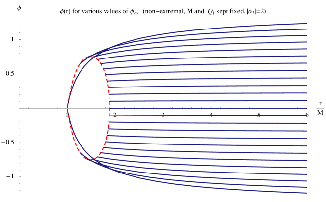
where $a_{0}$ and $a_{2}$ are non-trivial functions of $\bar{Q}_{i}$. Further details are discussed in section 9 and appendix B. The scalar field solutions for $\gamma=1$ and $2$ are illustrated in figs. 3 and 4 respectively.

4.2 Supersymmetry and the Exact Solutions

As mentioned above, the first two cases ($\gamma=1,2$) have been extensively studied in the literature.

The SUSY of the extremal $\alpha_{1}=-\alpha_{2}=2$ solution is discussed in [24]. They show that it is supersymmetric in the context of ${\cal N}=4$ SUGRA. It saturates the BPS bound and preserves $1\over 4$ of the supersymmetry - ie. it has ${\cal N}=1$ SUSY. There are BPS black-holes in this context which carry only one $U(1)$ charge and preserve $\frac{1}{2}$ of the supersymmetry. The non-extremal blackholes are of course non-BPS.

On the other hand, the extremal $\alpha_{1}=-\alpha_{2}=2\sqrt{3}$ blackhole is non-BPS [25]. It arises in the context of dimensionally reduced $5D$ Kaluza-Klein gravity [26] and is embeddable in ${\cal N}=2$ SUGRA. There however are BPS black-holes in this context which carry only one $U(1)$ charge and once again preserve $\frac{1}{2}$ of the supersymmetry [27].

We have not investigated the supersymmetry of the $\gamma=3$ solution, we expect that it is not a BPS solution in a supersymmetric theory.

5 General Higher Dimensional Analysis

5.1 The Set-Up

It is straightforward to generalise our results above to higher dimensions. We start with an action of the form,

$$S=\frac{1}{\kappa^{2}}\int d^{d}x\sqrt{-G}(R-2(\partial\phi_{i})^{2}-f_{ab}(\phi_{i})F^{a}F^{b})$$ (85)

Here the field strengths, $F_{a}$ are $(d-2)$ forms which are magnetic dual to $2$-form fields.

We will be interested in solution which preserve a $SO(d-2)$ rotation symmetry. Assuming all quantities to be function of $r$, and taking the charges to be purely magnetic, the ansatz for the metric and gauge fields is

$$ds^{2}=-a(r)^{2}dt^{2}+a(r)^{-2}dr^{2}+b(r)^{2}d\Omega_{d-2}^{2}$$ (86)

$$F^{a}=Q^{a}\sin^{d-3}\theta\sin^{d-4}\phi\cdots d\theta\wedge d\phi\wedge\cdots$$ (87)

$$\tilde{F}^{a}=Q^{a}\sin^{d-3}\theta\sin^{d-4}\phi\cdots d\theta\wedge d\phi\wedge\cdots$$ (88)

The equation of motion for the scalars is

$$\partial_{r}(a^{2}b^{d-2}\partial_{r}\phi_{i})=\frac{(d-2)!\partial_{i}V_{eff}}{4b^{d-2}}.$$ (89)

Here $V_{eff}$, the effective potential for the scalars, is given by

$$V_{eff}=f_{ab}(\phi_{i})Q^{a}Q^{b}.$$ (90)

From the $(R_{rr}-{G^{tt}\over G^{rr}}R_{tt})$ component of the Einstein equation we get,

$$\sum_{i}(\phi_{i}^{\prime})^{2}=-{(d-2)b^{\prime\prime}(r)\over 2b(r)}.$$ (91)

The $R_{rr}$ component gives the constraint,

$$\begin{array}[]{l}-(d-2)\{(d-3)-ab^{\prime}(2a^{\prime}b+(d-3)ab^{\prime})\}=2\phi_{i}^{\prime 2}a^{2}b^{2}-\frac{(d-2)!}{b^{2(d-3)}}V_{eff}(\phi_{i})\end{array}$$ (92)

In the analysis below we will use eq.(89) to solve for the scalars and then eq.(91) to solve for $b$. The constraint eq.(92) will be used in solving for $a$ along with one extra relation, $R_{tt}=(d-3){a^{2}\over b^{2}}R_{\theta\theta}$, as is explained in appendix C. These equations (aside from the constraint) can be derived from a one-dimensional action

$$\begin{array}[]{cccc}S&=&\frac{1}{\kappa^{2}}\int dr&\Big{(}(d-3)(d-2)b^{d-4}(1+a^{2}b^{{}^{\prime}2})+(d-2)b^{d-3}(a^{2})^{{}^{\prime}}b^{{}^{\prime}}\\ &&&-2a^{2}b^{d-2}(\partial_{r}\phi)^{2}-\frac{(d-2)!}{b^{d-2}}V_{eff}\Big{)}\end{array}$$ (93)

As the analysis below shows if the potential has a critical point at $\phi_{i}=\phi_{i0}$ and all the eigenvalues of the second derivative matrix $\partial_{ij}V(\phi_{i0})$ are positive then the attractor mechanism works in higher dimensions as well.

5.2 Zeroth and First Order Analysis

Our starting point is the case where the scalars take asymptotic values equal to their critical value, $\phi_{i}=\phi_{i0}$. In this case it is consistent to set the scalars to be a constant, independent of $r$. The extremal Reissner Nordstrom black hole in $d$ dimensions is then a solution of the resulting equations. This takes the form,

$$a_{0}(r)=\left(1-\frac{r_{H}^{d-3}}{r^{d-3}}\right)\quad b_{0}(r)=r$$ (94)

where $r_{H}$ is the horizon radius. From the eq.(92) evaluated at $r_{H}$ we obtain the relation,

$$r_{H}^{2(d-3)}=(d-4)!V_{eff}(\phi_{i0})$$ (95)

Thus the area of the horizon and the entropy of the black hole are determined by the value of $V_{eff}(\phi_{i0})$, as in the four-dimensional case.

Now, let us set up the first order perturbation in the scalar fields,

$$\phi_{i}=\phi_{i0}+\epsilon\phi_{i1}$$ (96)

The first order correction satisfies,

$$\partial_{r}(a_{0}^{2}b_{0}^{d-2}\partial_{r}\phi_{i1})=\frac{{\beta}_{i}^{2}}{b^{d-2}}\phi_{i1}$$ (97)

where, ${\beta}_{i}^{2}$ is the eigenvalue of the second derivative matrix ${(d-2)!\over 4}\partial_{ij}V_{eff}(\phi_{i0})$ corresponding to the mode $\phi_{i}$. This equation has two solutions. If ${\beta}_{i}^{2}>0$ one of these solutions blows up while the other is well defined and goes to zero at the horizon. This second solution is the one we will be interested in. It is given by,

$$\phi_{i1}=c_{i1}(1-{r_{H}^{d-3}/r^{d-3}})^{\gamma_{i}}$$ (98)

where $\gamma$ is given by

$$\gamma_{i}={\frac{1}{2}}\left(-1+{\sqrt{1+4{\beta}_{i}^{2}r_{H}^{6-2d}/(d-3)^{2}}}\right)$$ (99)

5.2.1 Second order calculations (Effects of backreaction)

The first order perturbation in the scalars gives rise to a second order correction for the metric components, $a,b$. We write,

$$b(r)=b_{0}(r)+\epsilon^{2}b_{2}(r)$$ (100)

$$a(r)^{2}=a_{0}(r)^{2}+\epsilon^{2}a_{2}(r)$$ (101)

$$b(r)^{2}=b_{0}(r)^{2}+2\epsilon^{2}b_{2}(r)b_{0}(r)$$ (102)

where $a_{0},b_{0}$ are given in eq.(94).

From (91) one can solve for the second order perturbation $b_{2}(r)$. For simplicity we consider the case of a single scalar field, $\phi$. The solution is given by double-integration form,

$${\partial_{r}^{2}b_{2}(r)} = -{\frac{2}{(d-2)}}r(\partial_{r}\phi_{1})^{2}=-c_{1}^{\prime}{\frac{1}{r^{2d-5}}}({\frac{{r^{d-3}-r_{H}^{d-3}}}{{r^{d-3}}}})^{2\gamma-2}$$

$$\Rightarrow b_{2}(r) = d_{1}r+d_{2}-{\frac{c_{1}^{\prime}r}{{2(d-3)(d-4)\gamma(2\gamma-1)r_{H}^{2d}}}}\times$$ (103)

$$\Bigl{(}-(d-4)F\left[{\textstyle{\frac{1}{{3-d}}},1-2\gamma,{\frac{{d-4}}{{d-3}}};({\frac{r_{H}}{r}})^{d-3}}\right]$$

$$+(2\gamma-1){\textstyle\left(\frac{r_{H}}{r}\right)^{d-3}}F\left[{\textstyle{\frac{{d-4}}{{d-3}}},1-2\gamma,{\frac{{2d-7}}{{d-3}}};({\frac{r_{H}}{r}})^{d-3}}\right]\Bigr{)}\,,$$

where $c_{1}^{\prime}\equiv 2(d-3)^{2}c_{1}^{2}\gamma^{2}r_{H}^{d}/(d-2)$, a positive definite constant, and $F$ is Gauss’s Hypergeometric function. More generally, for several scalar fields, $b_{2}$ is obtained by summing over the contributions from each scalar field. The integration constants $d_{1},d_{2}$, in eq.(103), can be fixed by coordinate transformations and requiring a double-zero horizon solution. We will choose coordinate so that the horizon is at $r=r_{H}$, then as we will see shortly the extremality condition requires both $d_{1},d_{2}$ to vanish. As $r\rightarrow r_{H}$ we have from eq.(103) that

$$b_{2}(r)\propto-\left({\frac{{r^{d-3}-r_{H}^{d-3}}}{{r^{d-3}}}}\right)^{2\gamma}$$ (104)

Since $\gamma>0$, we see that $b_{2}$ vanishes at the horizon and thus the area and the entropy are uncorrected to second order. At large $r$, $b_{2}(r)\propto{\mathcal{O}}(r)+{\mathcal{O}}(1)+{\mathcal{O}}(r^{7-2d})$ so asymptotic behaviour is consistent with asymptotic flatness of the solution.

The analysis for $a_{2}$ is discussed in more detail in appendix C. In the vicinity of the horizon one finds that there is one non-singular solution which goes like, $a_{2}(r)\rightarrow C(r-r_{H})^{(2\gamma+2)}$. This solution smoothly extends to $r\rightarrow\infty$ and asymptotically, as $r\rightarrow\infty$, goes to a constant which is consistent with asymptotic flatness.

Thus we see that the backreaction of the metric is finite and well behaved. A double-zero horizon black hole continues to exist to second order in perturbation theory. It is asymptotically flat. The scalars in this solution at the horizon take their attractor values irrespective of their values at infinity..

Finally, the analysis in principle can be extended to higher orders. Unlike four dimensions though an explicit solution for the higher order perturbations is not possible and we will not present such an higher order analysis here.

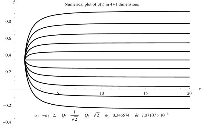
We end with Fig 5. which illustrates the attractor behaviour in asymptotically flat $4+1$ dimensional space. This figure has been obtained for the example, eq.(31, 32). The parameter $\delta r$ is defined in eq.(67).

Figure 5: Numerical plot of $\phi(r)$ with $\alpha_{1}=-\alpha_{2}=2$ for the an extremal black hole in $4+1$ dimensions displaying attractor behaviour.

6 Attractor in $AdS_{4}$

Next we turn to the case of Anti-de Sitter space in four dimensions. Our analysis will be completely analogous to the discussion above for the four and higher dimensional case and so we can afford to be somewhat brief below.

The action in 4-dim. has the form

$$S=\frac{1}{\kappa^{2}}\int d^{4}x\sqrt{-G}(R-2\Lambda-2(\partial\phi_{i})^{2}-f_{ab}(\phi_{i})F^{a}F^{b}-{\textstyle{1\over 2}}{\tilde{f}}_{ab}(\phi_{i})\epsilon^{\mu\nu\rho\sigma}F^{a}_{\mu\nu}F^{b}_{\rho\sigma})$$ (105)

where $\Lambda=-3/L^{2}$ is the cosmological constant. For simplicity we will discuss the case with only one scalar field here. The generalisation to many scalars is immediate and along the lines of the discussion for asymptotically flat four-dimensional case. Also we take the coefficient of the scalar kinetic energy term to be field independent.

For spherically symmetric solutions the metric takes the form, eq.(8). The field strengths are given by eq.(20). This gives rise to a one dimensional action

$$S=\frac{1}{\kappa^{2}}\int dr\left(2-(a^{2}b^{2})^{{}^{\prime\prime}}-2a^{2}bb^{{}^{\prime\prime}}-2a^{2}b^{2}(\partial_{r}\phi)^{2}-2\frac{V_{eff}}{b^{2}}+\frac{3b^{2}}{L^{2}}\right),$$ (106)

where $V_{eff}$ is given by eq.(21). The equations of motion, which can be derived either from eq.(106) or directly from the action, eq.(105) are now given by,

$$\partial_{r}(a^{2}b^{2}\partial_{r}\phi)=\frac{\partial_{\phi}V_{eff}(\phi)}{2b^{2}}$$ (107)

$$\frac{b^{{}^{\prime\prime}}}{b}=-(\partial_{r}\phi)^{2},$$ (108)

which are unchanged from the flat four-dimensional case, and,

$$(a^{2}(r)b^{2}(r))^{{}^{\prime\prime}}=2(1-2\Lambda b^{2}),$$ (109)

$$-1+a^{2}b^{{}^{\prime}2}+\frac{a^{2^{\prime}}b^{2^{\prime}}}{2}=\frac{-1}{b^{2}}(V_{eff}(\phi))+a^{2}b^{2}(\partial_{r}\phi)^{2}+\frac{3b^{2}}{L^{2}},$$ (110)

where the last equation is the first order constraint.

6.1 Zeroth and First Order Analysis for $V$

The zeroth order solution is obtained by taking the asymptotic values of the scalar field to be its critical values, $\phi_{0}$ such that $\partial_{i}V_{eff}(\phi_{0})=0$.

The resulting metric is now the extremal Reissner Nordstrom black hole in AdS space, [28], given by,

$$a_{0}(r)^{2} = {\frac{{(r-r_{H})^{2}(L^{2}+3r_{H}^{2}+2r_{H}r+r^{2})}}{{L^{2}r^{2}}}}$$ (111)

$$b_{0}(r) = r$$ (112)

The horizon radius $r_{H}$ is given by evaluating the constraint eq.(110) at the horizon,

$${\frac{{(L^{2}r_{H}^{2}+2r_{H}^{4})}}{{L^{2}}}}=V_{eff}(\phi_{0}).$$

The first order perturbation for the scalar satisfies the equation,

$$\partial_{r}(a_{0}^{2}b_{0}^{2}\partial_{r}\phi_{1})=\frac{{\beta}^{2}}{b^{2}}\phi_{1}$$ (114)

where,

$${\beta}^{2}={1\over 2}\partial_{\phi}^{2}V_{eff}(\phi_{0}).$$ (115)

This is difficult to solve explicitly.

In the vicinity of the horizon the two solutions are given by

$$\phi_{1}=C_{\pm}(r-r_{H})^{t_{\pm}}$$ (116)

If $V_{eff}^{\prime\prime}(\phi_{0})>0$ one of the two solutions vanishes at the horizon. We are interested in this solution. It corresponds to the choice,

$$\phi_{1}=C(r-r_{H})^{\gamma},$$ (117)

where,

$$\gamma=\frac{\sqrt{1+\frac{4{\beta}^{2}}{\delta r_{H}^{2}}}-1}{2},$$ (118)

and, $\delta={(L^{2}+6r_{H}^{2})\over L^{2}}$. As discussed in the appendix D this solution behaves at $r\rightarrow\infty$ as $\phi_{1}\rightarrow C_{1}+C_{2}/r^{3}$. Also, all other values of $r$, besides the horizon and $\infty$, are ordinary points of the second order equation eq.(114). All this establishes that there is one well-behaved solution for the first order scalar perturbation. In the vicinity of the horizon it takes the form eq.(116) with eq.(118), and vanishes at the horizon. It is non-singular everywhere between the horizon and infinity and it goes to a constant asymptotically at $r\rightarrow\infty$.

We consider metric corrections next. These arise at second order. We define the second order perturbations as in eq.(45). The equation for $b_{2}$ from the second order terms in eq.(108) takes the form,

$$b_{2}^{\prime\prime}=-r(\phi_{1}^{\prime}(r))^{2},$$ (119)

and can be solved to give,

$$b_{2}(r)=-\int_{r_{H}}\int_{r_{H}}[r(\phi_{1}^{\prime}(r))^{2}]$$ (120)

We fix the integration constants by taking take the lower limit of both integrals to be the horizon. We will see that this choice gives rise to an double-zero horizon solution. Since $\phi_{1}$ is well behaved for all $r_{H}\leq r\leq\infty$ the integrand above is well behaved as well. Using eq.(116) we find that in the near horizon region

$$b_{2}\sim(r-r_{H})^{(2\gamma)}$$ (121)

At $r\rightarrow\infty$ using the fact that $\phi_{1}\rightarrow C_{1}+C_{2}/r^{3}$ we find

$$b_{2}\sim D_{1}r+D_{2}+D_{3}/r^{6}.$$ (122)

This is consistent with an asymptotically AdS solution.

Finally we turn to $a_{2}$. As we show in appendix D a solution can be found for $a_{2}$ with the following properties. In the vicinity of the horizon it goes like,

$$a_{2}\propto(r-r_{H})^{(2\gamma+2)},$$ (123)

and vanishes faster than a double-zero. As $r\rightarrow\infty$, $a_{2}\rightarrow d_{1}r$ and grows more slowly than $a_{0}^{2}$. And for $r_{H}<r<\infty$ it is well-behaved and non-singular.

This establishes that after including the backreaction of the metric we have a non-singular, double-zero horizon black hole which is asymptotically AdS. The scalar takes a fixed value at the horizon of the black hole and the entropy of the black hole is unchanged as the asymptotic value of the scalar is varied.

Let us end with two remarks. In the AdS case one can hope that there is a dual description for the attractor phenomenon. Since the asymptotic value of the scalar is changing we are turning on a operator in the dual theory with a varying value for the coupling constant. The fact that the entropy, for fixed charge, does not change means that the number of ground states in the resulting family of dual theories is the same. This would be worth understanding in the dual description better. Finally, we expect this analysis to generalise in a straightforward manner to the AdS space in higher dimensions as well.

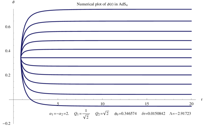
Fig. 6 illustrates the attractor mechanism in asymptotically $AdS_{4}$ space. This Figure is for the example, eq.(31, 32). The cosmological constant is taken to be, $\Lambda=-2.91723$, in $\kappa=1$ units.

Figure 6: Numerical plot of $\phi(r)$ with $\alpha_{1}=-\alpha_{2}=2$ for the an extremal black hole in $AdS_{4}$ displaying attractor behaviour.

7 Additional Comments

The theories we considered in the discussion of asymptotically flat space-times and AdS spacetimes have no potential for the scalars. We comment on this further here.

Let us consider a theory with ${\cal N}=1$ supersymmetry containing chiral superfields whose lowest component scalars are,

$$S_{i}=\phi_{i}+ia_{i}$$ (124)

We take these scalars to be uncharged under the gauge symmetries. These can be coupled to the superfields $W_{\alpha}^{a}$ by a coupling

$$L_{gaugekinetic}=\int d^{2}\theta f_{ab}(S_{i})W_{\alpha}^{a}W_{\alpha}^{b}$$ (125)

Such a coupling reproduces the gauge kinetic energy terms in and eq.(105), eq.(106), (we now include both $\phi_{i},a_{i}$ in the set of scalar fields which we denoted by $\phi_{i}$ in the previous sections).

An additional potential for the scalars would arise due to F-term contributions from a superpotential. If the superpotential is absent we get the required feature of no potential for these scalar. Setting the superpotential to be zero is at least technically natural due to its non-renormalisability.

In a theory with no supersymmetry there is no natural way to suppress a potential for the scalars and it would arise due to quantum effects even if it is absent at tree-level. In this case we have no good argument for not including a potential for the scalar and our analysis is more in the nature of a mathematical investigation.

The absence of a potential is important also for avoiding no-hair theorems which often forbid any scalar fields from being excited in black hole backgrounds [29]. In the presence of a mass $m$ in asymptotically flat four dimensional space the two solutions for first order perturbation at asymptotic infinity go like,

$$\phi\sim C_{1}e^{mr}/r,\phi\sim C_{2}e^{-mr}/r.$$ (126)

We see that one of the solutions blows up as $r\rightarrow\infty$. Since one solution to the equation of motion also blows up in the vicinity of the horizon, as discussed in section 2, there will generically be no non-singular solution in first order perturbation theory. This argument is a simple-minded way of understanding the absence of scalar hair for extremal black holes under discussion here. In the absence of mass terms, as was discussed in section 2, the two solutions at asymptotic infinity go like $\phi\sim{\rm const}$ and $\phi\sim 1/r$ respectively and are both acceptable. This is why one can turn on scalar hair. The possibility of scalar hair for a massless scalar is of course well known. See [30], [23], for some early examples of solutions with scalar hair, [31, 32, 33, 34], for theorems on uniqueness in the presence of such hair, and [8] for a discussion of resulting thermodynamics.

In asymptotic AdS space the analysis is different. Now the $(mass)^{2}$ for scalars can be negative as long as it is bigger than the BF bound. In this case both solutions at asymptotic infinity decay and are acceptable. Thus, as for the massless case, it should be possible to turn on scalar fields even in the presence of these mass terms and study the resulting black holes solutions. Unfortunately, the resulting equations are quite intractable. For small $(mass)^{2}$ we expect the attractor mechanism to continue to work.

If the $(mass)^{2}$ is positive one of the solutions in the asymptotic region blows up and the situation is analogous to the case of a massive scalar in flat space discussed above. In this case one could work with AdS space which is cut off at large $r$ (in the infrared) and study the attractor phenomenon. Alternatively, after incorporating back reaction, one might get a non-singular geometry which departs from AdS in the IR and then analyse black holes in this resulting geometry. In the dual field theory a positive $(mass)^{2}$ corresponds to an irrelevant operator. The growing mode in the bulk is the non-normalisable one and corresponds to turning on a operator in the dual theory which grows in the UV. Cutting off AdS space means working with a cut-off effective theory. Incorporating the back-reaction means finding a UV completion of the cut-off theory. And the attractor mechanism means that the number of ground states at fixed charge is the same regardless of the value of the coupling constant for this operator.

8 Asymptotic de Sitter Space

In de Sitter space the simplest way to obtain a double-zero horizon is to take a Schwarzschild black hole and adjust the mass so that the de Sitter horizon and the Schwarzschild horizon coincide. The resulting black hole is the extreme Schwarzschild-de Sitter spacetime [35]. We will analyse the attractor behaviour of this black hole below. The analysis simplifies in 5-dimensions and we will consider that case, a similar analysis can be carried out in other dimensions as well. Since no charges are needed we set all the gauge fields to zero and work only with a theory of gravity and scalars. Of course by turning on gauge charges one can get other double-zero horizon black holes in dS, their analysis is left for the future.

We start with the action of the form,

$$S=\frac{1}{\kappa^{2}}\int d^{5}x\sqrt{-G}(R-2(\partial\phi)^{2}-V(\phi))$$ (127)

Notice that the action now includes a potential for the scalar, $V(\phi)$, it will play the role of $V_{eff}$ in our discussion of asymptotic flat space and AdS space. The required conditions for an attractor in the dS case will be stated in terms of $V$. A concrete example of a potential meeting the required conditions will be given at the end of the section. For simplicity we have taken only one scalar, the analysis is easily extended for additional scalars.

The first condition on $V$ is that it has a critical point, $V^{\prime}(\phi_{0})=0$. We will also require that $V(\phi_{0})>0$. Now if the asymptotic value of the scalar is equal to its critical value, $\phi_{0}$, we can consistently set it to this value for all times $t$. The resulting equations have a extremal black hole solution mentioned above. This takes the form

$$ds^{2}=-{t^{2}\over(t^{2}/L-L/2)^{2}}dt^{2}+{(t^{2}/L-L/2)^{2}\over t^{2}}dr^{2}+t^{2}d\Omega_{3}^{2}$$ (128)

Notice that it is explicitly time dependent. $L$ is a length related to $V(\phi_{0})$ by , $V(\phi_{0})={20\over L^{2}}$. And $t=\pm{L\over\sqrt{2}}$ is the location of the double-zero horizon. A suitable near-horizon limit of this geometry is called the Nariai solution, [36].

8.1 Perturbation Theory

Starting from this solution we vary the asymptotic value of the scalar. We take the boundary at $t\rightarrow-\infty$ as the initial data slice and investigate what happens when the scalar takes a value different from $\phi_{0}$ as $t\rightarrow-\infty$. Our discussion will involve part of the space-time, covered by the coordinates in eq.(128), with $-\infty\leq t\leq t_{H}=-{L\over\sqrt{2}}$. We carry out the analysis in perturbation theory below.

Define the first order perturbation for the scalar by,

$$\phi=\phi_{0}+\epsilon\phi_{1}$$

This satisfies the equation,

$$\partial_{t}(a_{0}^{2}b_{0}^{3}\partial_{t}\phi_{1})={b^{3}\over 4}V^{\prime\prime}(\phi_{0})\phi_{1}$$ (129)

where $a_{0}={(t^{2}/L-L/2)\over t}$, $b_{0}=t$. This equation is difficult to solve in general.

In the vicinity of the horizon $t=t_{H}$, we have two solutions which go like,

$$\phi_{1}=C_{\pm}(t-t_{H})^{-1+\sqrt{1+\kappa^{2}}\over 2}$$ (130)

where

$$\kappa^{2}=-{1\over 4}V^{\prime\prime}(\phi_{0})$$ (131)

We see that one of the two solutions in eq.(130) is non-divergent and in fact vanishes at the horizon if

$$V^{\prime\prime}(\phi_{0})<0.$$ (132)

We will henceforth assume that the potential meets this condition. Notice this condition has a sign opposite to what was obtained for the asymptotically flat or AdS cases. This reversal of sign is due to the exchange of space and time in the dS case.

In the vicinity of $t\rightarrow-\infty$ there are two solutions to eq.(129) which go like,

$$\phi_{1}={\tilde{C}}_{\pm}|t|^{p_{\pm}}$$ (133)

where

$$p_{\pm}=2(-1\pm\sqrt{1+\kappa^{2}/4}).$$ (134)

If the potential meets the condition, eq.(132) then $\kappa^{2}>0$ and we see that one of the modes blows up at $t\rightarrow-\infty$.

8.2 Some Speculative Remarks

In view of the diverging mode at large $|t|$ one needs to work with a cutoff version of dS space . With such a cutoff at large negative $t$ we see that there is a one parameter family of solutions in which the scalar takes a fixed value at the horizon. The one parameter family is obtained by starting with the appropriate linear combination of the two solutions at $t\rightarrow-\infty$ which match to the well behaved solution in the vicinity of the horizon. While we will not discuss the metric perturbations and scalar perturbations at second order these too have a non-singular solution which preserves the double-zero nature of the horizon. The metric perturbations also grow at the boundary in response to the growing scalar mode and again the cut-off is necessary to regulate this growth. This suggests that in the cut-off version of dS space one has an attractor phenomenon. Whether such a cut-off makes physical sense and can be implemented appropriately are question we will not explore further here.

One intriguing possibility is that quantum effects implement such a cut-off and cure the infra-red divergence. The condition on the potential eq.(132) means that the scalar has a negative $(mass)^{2}$ and is tachyonic. In dS space we know that a tachyonic scalar can have its behaviour drastically altered due to quantum effects if it has a $(mass)^{2}<H^{2}$ where $H$ is the Hubble scale of dS space. This can certainly be arranged consistent with the other conditions on the potential as we will see below. In this case the tachyon can be prevented from “falling down” at large $|t|$ due to quantum effects and the infrared divergences can be arrested by the finite temperature fluctuations of dS space. It is unclear though if any version of of the attractor phenomenon survives once these quantum effects became important.

We end by discussing one example of a potential which meets the various conditions imposed above. Consider a potential for the scalar,

$$V=\Lambda_{1}e^{\alpha_{1}\phi}+\Lambda_{2}e^{\alpha_{2}\phi}.$$ (135)

We require that it has a critical point at $\phi=\phi_{0}$ and that the value of the potential at the critical point is positive. The critical point for the potential eq.(135) is at,

$$e^{\phi_{0}}=-\left({\alpha_{2}\Lambda_{2}\over\alpha_{1}\Lambda_{1}}\right)^{1\over\alpha_{1}-\alpha_{2}}$$ (136)

Requiring that $V(\phi_{0})>0$ tells us that

$$V(\phi_{0})=\Lambda_{2}e^{\alpha_{2}\phi_{0}}\left(1-{\alpha_{2}\over\alpha_{1}}\right)>0$$ (137)

Finally we need that $V^{\prime\prime}(\phi_{0})<0$ this leads to the condition,

$$V^{\prime\prime}(\phi_{0})=\Lambda_{2}e^{\alpha_{2}\phi_{0}}\alpha_{2}(\alpha_{2}-\alpha_{1})<0$$ (138)

These conditions can all be met by taking both $\alpha_{1},\alpha_{2}>0$, $\alpha_{2}<\alpha_{1}$, $\Lambda_{2}>0$ and $\Lambda_{1}<0$. In addition if $\alpha_{2}\alpha_{1}\gg 1$ the resulting $-(mass)^{2}\gg H^{2}$.

9 Non-Extremal = Unattractive

We end the paper by examining the case of an non-extremal black hole which has a single-zero horizon. As we will see there is no attractor mechanism in this case. Thus the existence of a double-zero horizon is crucial for the attractor mechanism to work.

Our starting point is the four dimensional theory considered in section 2 with action eq.(17). For simplicity we consider only one scalar field. We again start by consistently setting this scalar equal to its critical value, $\phi_{0}$, for all values of $r$, but now do not consider the extremal Reissner Nordstrom black hole. Instead we consider the non-extremal black hole which also solves the resulting equations. This is given by a metric of the form, eq.(8), with

$$a^{2}(r)=\left(1-{r_{+}\over r}\right)\left({1-{r_{-}\over r}}\right),\qquad b(r)=r$$ (139)

where $r_{\pm}$ are not equal. We take $r_{+}>r_{-}$ so that $r_{+}$ is the outer horizon which will be of interest to us.

The first order perturbation of the scalar field satisfies the equation,

$$\partial_{r}(a^{2}b^{2}\partial_{r}\phi_{i})={V_{eff}^{\prime\prime}(\phi_{0})\over 4b^{2}}\phi_{1}$$ (140)

In the vicinity of the horizon $r=r_{+}$ this takes the form,

$$\partial_{y}(y\partial_{y}\phi_{1})=\alpha\phi_{1}$$ (141)

where $\alpha$ is a constant dependent on $V^{\prime\prime}(\phi_{0}),r_{+},r_{-}$, and $y\equiv r-r_{+}$.

This equation has one non-singular solution which goes like,

$$\phi_{1}=C_{0}+C_{1}y+\cdots$$ (142)

where the ellipses indicate higher terms in the power series expansion of $\phi_{1}$ around $y=0$. The coefficients $C_{1},C_{2},\cdots$ are all determined in terms of $C_{0}$ which can take any value. Thus we see that unlike the case of the double-horizon extremal black hole, here the solution which is well-behaved in the vicinity of the horizon does not vanish.

Asymptotically, as $r\rightarrow\infty$ both solutions to eq.(140) are well defined and go like $1/r,constant$ respectively. It is then straightforward to see that one can choose an appropriate linear combination of the two solutions at infinity and match to the solution, eq.(142) in the vicinity of the horizon. The important difference here is that the value of the constant $C_{0}$ in eq.(142) depends on the asymptotic values of the scalar at infinity and therefore the value of $\phi$ does not go to a fixed value at the horizon. The metric perturbations sourced by the scalar perturbation can also be analysed and are non-singular. In summary, we find a family of non-singular black hole solutions for which the scalar field takes varying values at infinity. The crucial difference is that here the scalar takes a value at the horizon which depends on its value at asymptotic infinity. The entropy and mass for these solutions also depends on the asymptotic value of the scalar .

It is also worth examining this issue in a non-extremal black holes for an exactly solvable case.

If we consider the case $|\alpha_{i}|=2$, section 4, the non-extremal solution takes on a relatively simple form. It can be written[24]

$$\exp(2\phi) = e^{2\phi_{\infty}}\frac{(r+\Sigma)}{(r-\Sigma)}$$

$$a^{2} = \frac{(r-r_{+})(r-r_{-})}{(r^{2}-\Sigma^{2})}$$ (143)

$$b^{2} = (r^{2}-\Sigma^{2})$$

where

$$r_{\pm}=M\pm r_{0}\qquad r_{0}=\sqrt{M^{2}+\Sigma^{2}-\bar{Q}_{2}^{2}-\bar{Q}_{1}^{2}}.$$ (144)

and the Hamiltonian constraint becomes

$$\Sigma^{2}+M^{2}-\bar{Q}_{1}^{2}-\bar{Q}_{2}^{2}=\frac{1}{4}(r_{+}-r_{-})^{2}.$$ (145)

The scalar charge, $\Sigma$, defined by $\phi\sim\phi_{\infty}+\frac{\Sigma}{r}$, is not an independent parameter. It is given by

$$\Sigma=\frac{\bar{Q}_{2}^{2}-\bar{Q}_{1}^{2}}{2M}.$$ (146)

There are horizons at $r=r_{\pm}$, the curvature singularity occurs at $r=\Sigma$ and $r_{0}$ characterises the deviation from extremality. We see that the non-extremal solution does not display attractor behaviour.

Fig. 7 shows the behaviour of the scalar field as we vary $\phi_{\infty}$ keeping $M$ and $Q_{i}$ fixed. The location of the horizon as a function of $r$ depends on $\phi_{\infty}$, eq.(144). The horizon as a function of $\phi_{\infty}$ is denoted by the dotted line. The plot is terminated at the horizon.

In contrast, for the extremal black hole,

$$M=\frac{|\bar{Q}_{2}|+|\bar{Q}_{1}|}{\sqrt{2}}\qquad\Sigma=\frac{|\bar{Q}_{2}|-|\bar{Q}_{1}|}{\sqrt{2}},$$ (147)

so (9) gives

$$e^{2\phi_{0}}=e^{2\phi_{\infty}}\frac{M+\Sigma}{M-\Sigma}\stackrel{{\scriptstyle(\ref{eq:alpha2:Mass})}}{{=}}\frac{|Q_{2}|}{|Q_{1}|},$$ (148)

which is indeed the attractor value.

Figure 7: Plot $\phi(r)$ with $\alpha_{1}=-\alpha_{2}=2$ for the non-extremal black hole with $M,Q_{i}$ held fixed while varying $\phi_{\infty}$. The dotted line denotes the outer horizon at which we terminate the plot. It is clearly unattractive.

Acknowledgements

We thank A. Dabholkar, R. Gopakumar, G. Gibbons, S. Minwalla, A. Sen, M. Shigemori and A. Strominger for discussions. N.I. carried out part of this work while visiting Harvard University. He would like to thank the Harvard string theory group for its hospitality and support. We thank the organisers of ISM-04, held at Khajuraho, for a stimulating meeting. This research is supported by the Government of India. S.T. acknowledges support from the Swarnajayanti Fellowship, DST, Govt. of India. Most of all we thank the people of India for generously supporting research in String Theory.

Appendix A Perturbation Analysis

A.1 Mass

Here, we first calculate the mass of the extremal black hole discussed in section 2.2. From eq.(50), for large r, $b_{2}$ is given by,

$$b_{2}=cr+d$$ (A.1)

where

$$c = -\frac{c_{1}^{2}\gamma}{2(2\gamma-1)}$$ (A.2)

$$d = \frac{r_{H}c_{1}^{2}\gamma^{2}}{(2\gamma-1)}$$ (A.3)

Now, we can easily write down the expression for $a_{2}$ using eq.(48). We choose coordinate $y$ as introduced in eq.(51) such that at large r,

$$r^{2}+2\epsilon^{2}(cr^{2}+dr) = y^{2}$$ (A.4)

$$\frac{1}{r} = \frac{1}{y}(1+\epsilon^{2}(c+\frac{d}{y}))$$ (A.5)

We use the extremality condition (54) to find,

$$a(r)=\left(\frac{r-r_{H}}{y}\right)$$ (A.6)

Using, eq.(A.1, A.6) one finds that asymptotically, as $r\rightarrow\infty$ the metric takes the form,

$$ds^{2}=-\left(1-{2(r_{H}+\epsilon^{2}(cr_{H}+d))\over y}\right)d{\tilde{t}}^{2}+{1\over(1-{2(r_{H}+\epsilon^{2}(cr_{H}+d))\over y})}dy^{2}+y^{2}d\Omega^{2}$$ (A.7)

where ${\tilde{t}}$ is obtained by rescaling $t$ and $d\Omega^{2}$ denotes the metric of $S^{2}$. The mass $M$ of the black hole is then given by the $1/y$ term in the $g_{yy}$ component of the metric. This gives,

$$M=r_{H}+\epsilon^{2}\frac{r_{H}c_{1}^{2}\gamma}{2}.$$ (A.8)

A.2 Perturbation Series to All Orders

Next we go on to discuss the perturbation series to all orders, Using (55) for $b$ and (56) for $\phi$ in eq.(14)and eq.(62), we get,

$$b_{k}^{\prime\prime}=-\sum_{i=0}^{k}\sum_{j=0}^{k-i}b_{i}\phi_{j}^{\prime}\phi_{k-i-j}^{\prime}$$ (A.9)

$$\sum_{i+j\leqslant k}2b_{j}b_{k-i-j}((r-r_{H})^{2}\phi_{i}^{\prime})^{\prime}=Q_{i}^{2}e^{\alpha_{i}\phi_{0}}\alpha_{i}{\cal V}_{ik}$$ (A.10)

where

$${\cal V}_{ik} = \sum_{\stackrel{{\scriptstyle\{n_{1},n_{2}\ldots n_{k}\}}}{{\sum mn_{m}=k}}}\frac{\phi_{1}^{n_{1}}\phi_{2}^{n_{2}}\ldots\phi_{k}^{n_{k}}}{n_{1}!n_{2}!\ldots n_{k}!}\alpha^{n_{1}+n_{2}+\ldots+n_{k}}_{i}.$$ (A.11)

After substituting our ansatz (58)and (59), the above equations give,

$$k(k\gamma-1)d_{k}=-\gamma\sum_{{i+j<k}}j(k-i-j)d_{i}c_{j}c_{k-i-j}$$ (A.13)

and

$$k(k\gamma+1)c_{k}+T_{k}=(\gamma+1)(c_{k}+S_{k})$$ (A.14)

where $S_{k}$ and $T_{k}$ are given by

$$S_{k} = \sum_{\stackrel{{\scriptstyle\{n_{1},n_{2}\ldots n_{k-1}\}}}{{\sum mn_{m}=k}}}\frac{c_{1}^{n_{1}}c_{2}^{n_{2}}\ldots c_{k-1}^{n_{k-1}}}{n_{1}!n_{2}!\ldots n_{k-1}!}\left(\alpha^{\sum n_{l}-1}_{1}+\alpha^{\sum n_{l}-1}_{2}\right)$$ (A.15)

and

$$T_{k}=\sum_{\stackrel{{\scriptstyle j+l\leqslant k}}{{l<k}}}l(l\gamma+1)d_{j}d_{k-l-j}c_{l}.$$ (A.16)

Then solving for $d_{k}$ and $c_{k}$ gives

$$d_{k} = -\frac{\gamma}{k(k\gamma-1)}\sum_{{i+j<k}}j(k-i-j)d_{i}e_{j}e_{k-i-j}$$ (A.17)

$$c_{k} = \frac{(\gamma+1)S_{k}-T_{k}}{((k+1)\gamma+1)(k-1)}$$ (A.18)

Finally, $e_{k}$ can be obtained using eq.(54), eq.(59). It can be verified that the ansatz, eq.(58, 59, 60) with the coefficients eq.(A.17, A.18) also solves the constraint eq.(15).

Appendix B Exact Analysis

Exact solutions can be found by writing the equations of motion as generalised Toda equations [37], which may, in certain special cases, be solved exactly [23] - we rederive this result in slightly different notation below. As noted in [38], in a marginally different context, the extremal solutions, are, in appropriate variables, polynomial solutions of the Toda equations. The polynomial solutions are much easier to find and are related to the functions $f_{i}$ mentioned in section 4. For ease of comparison we occasionally use notation similar to [38].

B.1 New Variables

To recast the equations of motion into a generalised Toda equation we define the following new variables

$$u_{1}=\phi\qquad u_{2}=\log a\qquad z=\log ab\qquad\cdot=\partial_{\tau}=a^{2}b^{2}\partial_{r}$$ (B.1)

In terms of $r$, $\tau$ is given by

$$\tau=\int\frac{dr}{a^{2}b^{2}}=\frac{1}{(r_{+}-r_{-})}\log\left(\frac{r-r_{+}}{r-r_{-}}\right)$$ (B.2)

where $r_{\pm}$ are the integration constants of (13). In general (13) implies

$$a^{2}b^{2}=(r-r_{+})(r-r_{-}).$$ (B.3)

Notice that

$$\tau\rightarrow 0 r\rightarrow\infty$$ as (B.4)

$$\tau\rightarrow-\infty r\rightarrow r_{+}$$ as (B.5)

When we have a double-zero horizon, $r_{H}=r_{\pm}$, $\tau$ takes the simple form

$$\tau^{-1}=-{\left(r-r_{H}\right)}.$$ (B.6)

Since we are mainly interested in solutions with double-zero horizons, in what follows it will be convenient to work with a new radial coordinate, $\rho$, defined by

$$\rho=-\tau^{-1}.$$ (B.7)

which has the convenient property that $\rho_{H}=0$.

B.2 Equivalent Toda System

In terms of these new variables the equations of motion become

$$\ddot{u}_{1} = {\textstyle{\frac{1}{2}}}\alpha_{1}e^{2u_{2}+\alpha_{1}u_{1}}Q_{1}^{2}+{\textstyle{\frac{1}{2}}}\alpha_{2}e^{2u_{2}+\alpha_{2}u_{1}}Q_{2}^{2}$$ (B.8)

$$\ddot{u}_{2} = e^{2u_{2}+\alpha_{1}u_{1}}Q_{1}^{2}+e^{2u_{2}+\alpha_{2}u_{1}}Q_{2}^{2}$$ (B.9)

$$\ddot{z} = e^{2z}$$ (B.10)

$$\dot{u_{1}}^{2}+\dot{u_{2}}^{2}-\dot{z}^{2}+e^{2z}-e^{2u_{2}+\alpha_{1}u_{1}}Q_{1}^{2}-e^{2u_{2}+\alpha_{2}u_{1}}Q_{2}^{2}=0$$ (B.11)

(B.10) decouples from the other equations and is equivalent to (13). Finally making the coordinate change

$$X_{i}=n_{ij}^{-1}u_{j}+m_{ij}^{-1}\log\left((\alpha_{1}-\alpha_{2})Q_{j}^{2}\right)$$ (B.12)

where

$$n^{-1}=\left(\begin{array}[]{cc}2&-\alpha_{2}\\ -2&\alpha_{1}\end{array}\right)$$ (B.13)

and

$$m_{ij}=\frac{1}{2\left(\alpha_{1}-\alpha_{2}\right)}\left(4+\alpha_{i}\alpha_{j}\right)$$ (B.14)

we obtain the generalised 2 body Toda equation

$$\ddot{X}_{i}=e^{m_{ij}X_{j}},$$ (B.15)

together with

$$\sum_{ij}\left(\textstyle\frac{1}{2}\dot{X}_{i}m_{ij}\dot{X}_{j}-e^{m_{ij}X_{j}}\right)=(\alpha_{1}-\alpha_{2})\mathcal{E}$$ (B.16)

where ${\cal E}=\frac{1}{4}(r_{+}-r_{-})^{2}$. After solving the above, the original fields will be given by

$$e^{(\alpha_{1}-\alpha_{2})\phi} = \frac{Q_{2}^{2}}{Q_{1}^{2}}e^{\frac{1}{2}(\alpha_{1}X_{1}+\alpha_{2}X_{2})}$$ (B.17)

$$a^{2} = e^{\frac{2}{\alpha_{1}-\alpha_{2}}(X_{1}+X_{2})}/\diamondsuit$$ (B.18)

$$b^{2} \stackrel{{\scriptstyle(\ref{eq1})}}{{=}} (r-r_{+})(r-r_{-})/a^{2}$$ (B.19)

where

$$\diamondsuit=(\alpha_{1}-\alpha_{2})Q_{1}^{2\frac{-\alpha_{2}}{\alpha_{1}-\alpha_{2}}}Q_{2}^{2\frac{\alpha_{1}}{\alpha_{1}-\alpha_{2}}}$$ (B.20)

B.3 Solutions

B.3.1 Case I: $\gamma=1\Leftrightarrow\alpha_{1}\alpha_{2}=-4$

In this case, $m_{ij}$ is diagonal

$$m=\mathrm{diag}(\alpha_{1}/2,-\alpha_{2}/2),$$ (B.21)

so the equations of motion decouple:

$$\ddot{X}_{i}=e^{\frac{|\alpha_{i}|}{2}X_{i}}.$$ (B.22)

(B.22) has solutions

$$X_{i}=\frac{2}{|\alpha_{i}|}\log\left(\frac{4c_{i}^{2}}{|\alpha_{i}|\sinh^{2}(c_{i}(\tau-d_{i}))}\right)$$ (B.23)

The integration constants are fixed by imposing asymptotic boundary conditions and requiring that the solution is finite at the horizon. Letting

$$F_{i}=\sinh(c_{i}\left(\tau-d_{i}\right))$$ (B.24)

in terms of $\phi$ and $a$ we get

$$\begin{array}[]{cll}e^{(\alpha_{1}-\alpha_{2})\phi}&=&\displaystyle\frac{Q_{2}^{2}}{Q_{1}^{2}}e^{\frac{1}{2}(\alpha_{1}X_{1}+\alpha_{2}X_{2})}\\ &=&\displaystyle\left(-\frac{\alpha_{2}}{\alpha_{1}}\right)\left(\frac{Q_{2}F_{2}c_{1}}{Q_{1}F_{1}c_{2}}\right)^{2}\\ a^{2}&=&\displaystyle\left.e^{\frac{2}{\alpha_{1}-\alpha_{2}}(X_{1}+X_{2})}\right/\diamondsuit\\ &=&\displaystyle\left.\left(\frac{c_{1}}{Q_{1}F_{1}}\right)^{2\frac{-\alpha_{2}}{\alpha_{1}-\alpha_{2}}}\left(\frac{c_{2}}{Q_{2}F_{2}}\right)^{2\frac{\alpha}{\alpha-\tilde{\alpha}}}\right/\spadesuit\end{array}$$ (B.25)

As $r\rightarrow r_{+}$(ie. $\tau\rightarrow-\infty$) the scalar field goes like

$$e^{(\alpha_{1}-\alpha_{2})\phi}\sim e^{2(c_{1}-c_{2})\tau}\\$$ (B.26)

so we require

$$c:=c_{1}=c_{2}$$ (B.27)

for a finite solution at the horizon. Also at the horizon

$$b^{2}\sim(r-r_{+})/a^{2}\sim e^{\left((r_{+}-r_{-})-2c\right)\tau}$$ (B.28)

which necessitates

$$(r_{+}-r_{-})=2c$$ (B.29)

To find the extremal solutions we take the limit $c\rightarrow 0$ which gives

$$e^{(\alpha_{1}-\alpha_{2})\phi} = \left(-\frac{\alpha_{2}}{\alpha_{1}}\right)\frac{\left(Q_{2}f_{2}\right)^{2}}{\left(Q_{1}f_{1}\right)^{2}}$$ (B.30)

$$b^{2} = \spadesuit\left(Q_{1}f_{1}\right)^{\frac{-2{\alpha_{2}}}{\alpha_{1}-\alpha_{2}}}\left(Q_{2}p_{2}\right)^{\frac{2\alpha_{1}}{\alpha_{1}-\alpha_{2}}}$$ (B.31)

$$a^{2} = \rho^{2}/b^{2}$$ (B.32)

where

$$f_{i}=1+d_{i}\rho.$$ (B.33)

Requiring $\phi\rightarrow\phi_{\infty}$ and $a\rightarrow 1$ as $r\rightarrow\infty$ fixes

$$d_{i}=\bar{Q_{i}}^{-1}\sqrt{\frac{|\alpha_{i}|}{\alpha_{1}-\alpha_{2}}}$$ (B.34)

where as before

$$\bar{Q}_{i}^{2}=e^{\alpha_{i}\phi_{\infty}}Q_{i}^{2}\qquad\mbox{(no summation)}.$$ (B.35)

For comparison with the non-extremal solution in this case see section 9.

B.3.2 Case II: $\gamma=2$ and $\alpha_{1}=-\alpha_{2}=2\sqrt{3}$

In this case, $m_{ij}$ becomes

$$m=\left(\matrix{\frac{2}{{\sqrt{3}}}&-\frac{1}{{\sqrt{3}}}\cr-\frac{1}{{\sqrt{3}}}&\frac{2}{{\sqrt{3}}}\cr}\right).$$ (B.36)

It is convenient to use the coordinates

$$q_{i}=\frac{1}{\sqrt{3}}X_{i}-\sqrt{3}\log\sqrt{3}$$ (B.37)

so the equations of motion are the two particle Toda equations

$$\ddot{q}_{1} = e^{2q_{1}-q_{2}}$$ (B.38)

$$\ddot{q}_{2} = e^{2q_{2}-q_{1}}.$$ (B.39)

These maybe integrated exactly but the explicit form is, in general, a little complicated. Fortunately we are mainly interested in extremal solutions which have a simpler form [38]. As in, [38], taking the ansatz that $e^{-q_{i}}$ is a second order polynomial one finds

$$e^{-q_{1}} = a_{0}+a_{1}\tau+\frac{1}{2}\tau^{2}$$ (B.40)

$$e^{-q_{2}} = a_{1}^{2}-a_{0}+a_{1}\tau+\frac{1}{2}\tau^{2}$$ (B.41)

Finally, returning to the original variables and imposing the asymptotic boundary conditions gives the solution

$$e^{4\sqrt{3}\phi} = \left(\frac{Q_{2}}{Q_{1}}\right)^{2}\left(\frac{f_{2}}{f_{1}}\right)^{6}$$ (B.42)

$$b^{2} = 2Q_{1}Q_{2}f_{1}f_{2}$$ (B.43)

$$a^{2} = \rho^{2}/b^{2}$$ (B.44)

where

$$f_{i}=\left(1+(\bar{Q}_{1}\bar{Q}_{2})^{-\frac{2}{3}}(\bar{Q}_{1}^{\frac{2}{3}}+\bar{Q_{2}}^{\frac{2}{3}})^{\frac{1}{2}}\rho+{\textstyle\frac{1}{2}}(\bar{Q}_{i}\bar{Q}_{1}\bar{Q}_{2})^{-\frac{2}{3}}\rho^{2}\right)^{\frac{1}{2}}$$ (B.45)

as quoted in section 4.

For completeness we note that the general, non-extremal solution of [26, 30], modified for a non-zero asymptotic value of $\phi$, is

$$\exp(4\phi/\sqrt{3}) =e^{4\phi_{\infty}/\sqrt{3}} \frac{p_{2}}{p_{1}}$$ (B.46)

$$a^{2} = \frac{(r-r_{+})(r-r_{-})}{\sqrt{p_{1}p_{2}}}$$ (B.47)

$$b^{2} = \sqrt{p_{1}p_{2}}$$ (B.48)

where

$$p_{i}=(r-r_{i+})(r-r_{i-})$$ (B.49)

$$r_{i\pm}=\frac{2}{(-\alpha_{i})}\Sigma\pm\bar{Q}_{i}\sqrt{\frac{4\Sigma}{2\Sigma+\alpha_{i}M}}$$ (B.50)

and scalar charge, $\Sigma$, which is again not an independent parameter, is given by

$$\frac{1}{\sqrt{3}}\Sigma=\frac{\bar{Q}_{2}^{2}}{2M(\lambda-1)}+\frac{\bar{Q}_{1}^{2}}{2M(\lambda+1)}\qquad\lambda=\frac{\Sigma}{\sqrt{3}M}$$ (B.51)

B.3.3 Case III: $\gamma=3$ and $\alpha_{1}=4\qquad\alpha_{2}=-6$

In this case, $m_{ij}$ becomes

$$m=\left(\begin{array}[]{cc}1&-1\\ -1&2\end{array}\right)$$ (B.52)

Making the coordinate change

$$q_{1} = {\textstyle{\frac{1}{2}}}X_{1}-\log 2$$ (B.53)

$$q_{2} = X_{2}-\log 2$$ (B.54)

The equations of motion are

$$\ddot{q}_{1} = e^{2q_{1}-q_{2}}$$ (B.55)

$$\ddot{q}_{2} = e^{2q_{2}-2q_{2}}$$ (B.56)

Now consider the three particle Toda system

$$\ddot{q}_{1} = e^{2q_{1}-q_{2}}$$ (B.57)

$$\ddot{q}_{2} = e^{2q_{2}-q_{1}-q_{3}}$$ (B.58)

$$\ddot{q}_{3} = e^{2q_{3}-q_{2}}$$ (B.59)

which may be integrated exactly. Notice that by identifying $q_{1}$ and $q_{3}$ we obtain (B.57-B.59). Once again the general solution is slightly complicated but taking the ansatz that $e^{-q_{i}}$ is a polynomial one finds

$$e^{-q_{1}} = a_{0}+2a_{2}^{2}\tau+a_{2}\tau^{2}+\frac{1}{6}\tau^{3}$$ (B.60)

$$e^{-q_{2}} = 4a_{2}^{4}-2a_{0}a_{2}+(4a_{2}^{3}-a_{0})\tau+2a_{2}^{2}\tau^{2}+\frac{2}{3}a_{2}\tau^{3}+\frac{1}{12}\tau^{4}$$ (B.61)

Rewriting in terms of the original fields we get

$$e^{10\phi} = \left(\frac{Q_{2}}{Q_{1}}\right)^{2}\exp\left(2X_{1}-3X_{2}\right)$$ (B.62)

$$= \frac{6}{4}\left(\frac{Q_{2}}{Q_{1}}\right)^{2}\left(\frac{f_{2}}{f_{1}}\right)^{12}$$ (B.63)

$$b^{2} = \rho^{2}10Q_{1}^{\frac{6}{5}}Q_{2}^{\frac{4}{5}}\exp\left(-\frac{1}{5}X_{1}-\frac{1}{5}X_{2}\right)$$ (B.64)

$$= \frac{5}{2}\left(\frac{2}{3}\right)^{\frac{3}{5}}Q_{1}^{\frac{6}{5}}Q_{2}^{\frac{4}{5}}f_{1}f_{2}$$ (B.65)

$$a^{2} = \rho^{2}/b^{2}$$ (B.66)

where

$$f_{1}=\left(1-6a_{2}\rho+12a_{2}^{2}\rho^{2}-6a_{0}\rho^{3}\right)^{\frac{1}{3}}$$ (B.67)

$$f_{2}=\left(1-{\textstyle\frac{24}{3}}a_{2}\rho+24a_{2}\rho^{2}-(48a_{2}^{3}-12a_{0})\rho^{3}+\left(48a_{2}^{4}-24a_{0}a_{2}\right)\rho^{4}\right)^{\frac{1}{4}}$$ (B.68)

At the horizon we do indeed have $\phi$ at the critical point of $V_{eff}$:

$$e^{10\phi_{0}}=\frac{3}{2}\frac{Q_{2}^{2}}{Q_{1}^{2}}$$ (B.69)

and $b^{2}$ given by $V_{eff}(\phi_{0})$:

$$b_{H}^{2}=\frac{5}{2}\left(\frac{2}{3}\right)^{\frac{3}{5}}Q_{1}Q_{2}\left(\frac{Q_{2}}{Q_{1}}\right)^{\frac{1}{5}}.$$ (B.70)

Imposing the asymptotic boundary conditions we get

$$a_{0}=\pm\frac{2^{\frac{5}{7}}}{\bar{Q}_{1}^{\frac{10}{7}}\bar{Q}_{2}^{\frac{5}{7}}}\qquad\left(4a_{2}^{4}-2a_{0}a_{2}\right)=\frac{2^{\frac{11}{7}}}{\bar{Q}_{1}^{\frac{22}{7}}\bar{Q}_{2}^{\frac{18}{7}}}$$ (B.71)

so letting

$$\clubsuit = \frac{2^{\frac{11}{7}}}{Q_{1}^{\frac{22}{7}}Q_{2}^{\frac{18}{7}}}$$ (B.72)

$$\Delta_{1} = 3\sqrt[3]{a_{0}^{3}+\sqrt{a_{0}^{6}+\frac{64}{3}a_{0}^{3}\clubsuit^{3}}}$$ (B.73)

$$\Delta_{2} = \sqrt{\frac{3^{\frac{1}{3}}\Delta_{1}}{a_{0}}-\frac{3^{\frac{2}{3}}4}{\Delta_{1}}}$$ (B.74)

we may write $a_{2}$ as

$$a_{2}=\pm\frac{1}{2\sqrt{6}}\Delta_{2}\pm\frac{1}{2}\sqrt{\frac{2\clubsuit}{3^{\frac{1}{3}}\Delta_{1}}-\frac{\Delta_{1}}{2\,3^{\frac{2}{3}}}+\frac{\sqrt{6}}{\Delta_{2}}}$$ (B.75)

Despite the non-trivial form of the solution we see that it still takes on the attractor value at the horizon.

In terms of the $U(1)$ charges (written implicitly in terms of $a_{0}$ and $a_{2}$), the mass and scalar charge are expressed below

$$\Sigma=\frac{3a_{0}^{2}-28a_{0}a_{2}^{3}+32a_{2}^{6}}{40a_{0}a_{2}^{4}-20a_{0}^{2}a_{2}}$$ (B.76)

$$M=\frac{(a_{0}^{2}+4a_{0}a_{2}^{3}-16a_{2}^{6})}{2^{\frac{3}{5}}50a_{0}^{\frac{7}{5}}a_{2}(a_{0}-2a_{2}^{3})(2a_{2}^{4}-a_{0}a_{2})^{\frac{1}{5}}Q_{1}^{\frac{6}{5}}Q_{2}^{\frac{4}{5}}}$$ (B.77)

This solution is related to a 3 charge p-brane solution found in [38] - in this case we have identified two of the degrees of freedom.

Appendix C Higher Dimensions

Here we give some more details related to our discussion of the higher dimensional attractor in section 5. The Ricci components calculated from the metric, eq.(86) are,

$$R_{tt} = a^{2}\left(a^{\prime 2}+{\frac{{(d-2)aa^{\prime}b^{\prime}}}{{b}}}+aa^{\prime\prime}\right)$$ (C.1)

$$R_{rr} = -\{b\left(a^{\prime 2}+aa^{\prime\prime}\right)+(d-2)a\left(a^{\prime}b^{\prime}+ab^{\prime\prime}\right)\}/a^{2}b$$ (C.2)

$$R_{\theta\theta} = (d-3)-2aba^{\prime}b^{\prime}-a^{2}\left((d-3)b^{\prime 2}+bb^{\prime\prime}\right)$$ (C.3)

The Einstein equations from the action eq.(85), take the form,

$$R_{tt} = \frac{(d-3)(d-3)!a(r)^{2}}{b(r)^{2(d-2)}}V_{eff}(\phi_{i})$$ (C.4)

$$R_{rr} = 2(\partial_{r}\phi)^{2}-\frac{(d-3)(d-3)!}{b(r)^{2(d-2)}a(r)^{2}}V_{eff}(\phi_{i})$$

$$R_{\theta\theta} = \frac{(d-3)!}{b^{2(d-3)}}V_{eff}(\phi_{i}),$$ (C.6)

where $V_{eff}$ is given by eq.(90).

Taking the combination, ${1\over 2}(R_{rr}-{G_{rr}\over G_{tt}}R_{tt})$ gives, eq.(91). Similarly we have,

$${\frac{b(r)^{2}}{a(r)^{2}}}R_{tt}+a(r)^{2}b(r)^{2}R_{rr}-(d-2)R_{\theta\theta}$$ (C.7)

$$= -(d-2)\{d-3-a(r)b^{\prime}(r)(2a^{\prime}(r)b(r)+(d-3)a(r)b^{\prime}(r))\}$$

$$= 2(\partial_{r}\phi_{i})^{2}a(r)^{2}b(r)^{2}-\frac{(d-2)(d-3)!}{b^{2(d-3)}}V_{eff}(\phi_{i})\$$

This gives eq.(92). Finally the relation, $R_{tt}=(d-3){a^{2}\over b^{2}}R_{\theta\theta}$ yields,

$$(d-3)^{2}(-1+a(r)^{2}b^{\prime}(r)^{2})+b(r)^{2}(a^{\prime}(r)^{2}+a(r)a^{\prime\prime}(r))$$

$$+a(r)b(r)((-8+3d)a^{\prime}(r)b^{\prime}(r)+(d-3)a(r)b^{\prime\prime}(r))=0.$$ (C.8)

We now discuss solving for $a_{2}$, the second order perturbation in the metric component $a$, in some more detail. We restrict ourselves to the case of one scalar field, $\phi$. The constraint, eq.(92), to $O(\epsilon^{2})$ is,

$$(d-2)ra_{2}^{\prime}+(d-2)(d-3)a_{2}-2(\phi_{1}^{\prime})^{2}r^{2}(1-(\frac{r_{H}}{r})^{d-3})^{2}$$ (C.9)

$$-2(d-2)(d-3)^{2}\frac{r_{H}^{2(d-3)}}{r^{2(d-3)+1}}b_{2}+2(d-3)^{2}\frac{\gamma(\gamma+1)\phi_{1}^{2}}{r^{2(d-3)}r_{H}^{6-2d}}$$

$$+2(d-2)\frac{(d-3)(r_{H}^{3}r^{d}-r_{h}^{d}r^{3})}{r_{H}^{6}r^{2d}}\left\{r_{H}^{d}r^{2}b_{2}+r_{h}^{3}r^{d}b_{2}^{\prime}\right\}=0$$

This is a first order equation for $a_{2}$ of the form,

$$f_{1}a_{2}^{\prime}+f_{2}a_{2}+f_{3}=0,$$ (C.10)

where,

$$f_{1} = (d-2)r$$

$$f_{2} = (d-2)(d-3)$$

$$f_{3} = -2(\phi_{1}^{\prime})^{2}r^{2}(1-(\frac{r_{H}}{r})^{d-3})^{2}-2(d-2)(d-3)^{2}\frac{r_{H}^{2(d-3)}}{r^{2(d-3)+1}}b_{2}$$ (C.11)

$$+2(d-3)^{2}\frac{t(t+1)\phi_{1}^{2}}{r^{2(d-3)}r_{H}^{6-2d}}$$

$$+2(d-2)\frac{(d-3)(r_{H}^{3}r^{d}-r_{H}^{d}r^{3})}{r_{H}^{6}r^{2d}}\left\{r_{H}^{d}r^{2}b_{2}+r_{H}^{3}r^{d}b_{2}^{\prime}\right\}$$

The solution to this equation is given by,

$$a_{2}(r)=Ce^{\mathcal{F}}-e^{\mathcal{F}}\int e^{-\mathcal{F}}\frac{f_{3}}{f_{1}}dr$$ (C.12)

where $\mathcal{F}=-\int\frac{f_{2}}{f_{1}}dr$. It is helpful to note that $e^{\mathcal{F}}={1\over r^{(d-3)}}$ and, $\frac{e^{-\mathcal{F}}}{f_{1}}={r^{d-4}\over(d-2)}$.

Now the first term in eq.(C.12), proportional to $C$, blows up at the horizon. We will omit some details but it is easy to see that the second term in eq.(C.12) goes to zero. Thus for a non-singular solution we must set $C=0$. One can then extract the leading behaviour near the horizon of $a_{2}$ from eq.(C.12), however it is slightly more convenient to use eq.(C.8) for this purpose instead. From the behaviour of the scalar perturbation $\phi_{1}$, and metric perturbation, $b_{2}$, in the vicinity of the horizon, as discussed in the section on attractors in higher dimensions, it is easy to see that

$$a_{2}(r)=A_{2}(r^{d-3}-r_{H}^{d-3})^{2\gamma+2}$$ (C.13)

where, $A_{2}$ is an appropriately determined constant. Thus we see that the non-singular solution in the vicinity of the horizon vanishes like $(r-r_{H})^{(2\gamma+2)}$ and the double-zero nature of the horizon persists after including back-reaction to this order.

Finally, expanding eq.(C.12) near $r\rightarrow\infty$ (with $C=0$) we get that $a_{2}\rightarrow{\rm Const}+{\mathcal{O}}(1/r^{d-3})$. The value of the constant term is related to the coefficient in the linear term for $b_{2}$ at large $r$ in a manner consistent with asymptotic flatness.

In summary we have established here that the metric perturbation $a_{2}$ vanishes fast enough at the horizon so that the black hole continues to have a double-zero horizon, and it goes to a constant at infinity so that the black hole continues to be asymptotically flat.

Appendix D More Details on Asymptotic AdS Space

We begin by considering the asymptotic behaviour at large $r$ of $\phi_{1}$, eq.(114). One can show that this is given by

$$\phi_{1}(r)\rightarrow c_{+}{\frac{1}{r^{3/2}}}I_{3/4}\left(\frac{{\beta}L}{2r^{2}}\right)+c_{-}{\frac{1}{r^{3/2}}}I_{-3/4}\left(\frac{{\beta}L}{2r^{2}}\right)$$ (D.1)

Here $I_{3/4}$ stands for a modified Bessel function Asymptotically, $I_{\nu}\propto r^{-2\nu}$. Thus $\phi_{r}$ has two solutions which go asymptotically to a constant and as $1/r^{3}$ respectively.

Next, we consider values of r, $r_{H}<r<\infty$. These are all ordinary points of the differential equation eq.(114). Thus the solution we are interested is well-behaved at these points. For a differential equation of the form,

$$\mathcal{L}(\psi)=\frac{d^{2}\psi}{dz^{2}}+p(z)\frac{d\psi}{dz}+q(z)\psi=0,$$ (D.3)

all values of $z$ where $p(z),q(z)$ are analytic are ordinary points. About any ordinary point the solutions to the equation can be expanded in a power series, with a radius of convergence determined by the nearest singular point [22].

We turn now to discussing the solution for $a_{2}$. The constraint eq.(110) takes the form,

$$2a_{0}^{2}b_{2}^{\prime}+a_{2}+(a_{0}^{2})^{\prime}(rb_{2})^{\prime}+ra_{2}^{\prime}=\frac{-1}{r^{2}}{\beta}^{2}\phi_{1}^{2}+a_{0}^{2}r^{2}(\partial_{r}\phi_{1})^{2}+{2b_{2}\over r^{3}}(r_{H}^{2}+{2r_{H}^{4}\over L^{2}})+\frac{6rb_{2}}{L^{2}}$$ (D.4)

The solution to this equation is given by,

$$a_{2}(r)=\frac{c_{2}}{r}-\frac{1}{r}\int_{r_{H}}f_{3}dr$$ (D.5)

where

$$f_{3}=2a_{0}^{2}b_{2}^{\prime}+(a_{0}^{2})^{\prime}(rb_{2})^{\prime}+\frac{1}{r^{2}}\beta^{2}\phi_{1}^{2}-a_{0}^{2}r^{2}(\partial_{r}\phi_{1})^{2}-{2b_{2}\over r^{3}}(r_{H}^{2}+{2r_{H}^{4}\over L^{2}})-\frac{6rb_{2}}{L^{2}}$$ (D.6)

. We have set the lower limit of integration in the second term at $r_{H}$. We want a solution the preserves the double-zero structure of the horizon. This means $c_{2}$ must be set to zero.

To find an explicit form for $a_{2}$ in the near horizon region it is slightly simpler to use the equation, eq.(109). In the near horizon region this can easily be solved and we find the solution,

$$a_{2}\propto(r-r_{H})^{(2\gamma+2)}.$$ (D.7)

At asymptotic infinity one can use the integral expression, eq.(D.5) (with $c_{2}=0$). One finds that $f_{3}\rightarrow r$ as $r\rightarrow\infty$. Thus $a_{2}\rightarrow d_{2}r$. This is consistent with the asymptotically AdS geometry.

In summary we see that that there is an attractor solution to the metric equations at second order in which the double-zero nature of the horizon and the asymptotically AdS nature of the geometry both persist.

References

- [1] S. Ferrara, R. Kallosh and A. Strominger, Phys. Rev. D 52, R5412 (1995) [arXiv:hep-th/9508072].
- [2] M. Cvetic and A. A. Tseytlin, Phys. Rev. D 53, 5619 (1996) [Erratum-ibid. D 55, 3907 (1997)] [arXiv:hep-th/9512031].
- [3] A. Strominger, Phys. Lett. B 383, 39 (1996) [arXiv:hep-th/9602111].
- [4] S. Ferrara and R. Kallosh, Phys. Rev. D 54, 1514 (1996) [arXiv:hep-th/9602136].
- [5] S. Ferrara and R. Kallosh, Phys. Rev. D 54, 1525 (1996) [arXiv:hep-th/9603090].
- [6] M. Cvetic and C. M. Hull, Nucl. Phys. B 480, 296 (1996) [arXiv:hep-th/9606193].
- [7] S. Ferrara, G. W. Gibbons and R. Kallosh, Nucl. Phys. B 500, 75 (1997) [arXiv:hep-th/9702103].
- [8] G. W. Gibbons, R. Kallosh and B. Kol, Phys. Rev. Lett. 77, 4992 (1996) [arXiv:hep-th/9607108].
- [9] F. Denef, JHEP 0008, 050 (2000) [arXiv:hep-th/0005049].
- [10] F. Denef, B. R. Greene and M. Raugas, JHEP 0105, 012 (2001) [arXiv:hep-th/0101135].
- [11] H. Ooguri, A. Strominger and C. Vafa, Phys. Rev. D 70, 106007 (2004) [arXiv:hep-th/0405146].
- [12] G. Lopes Cardoso, B. de Wit and T. Mohaupt, Phys. Lett. B 451, 309 (1999) [arXiv:hep-th/9812082].
- [13] A. Dabholkar, [arXiv:hep-th/0409148].
- [14] H. Ooguri, C. Vafa and E. P. Verlinde, [arXiv:hep-th/0502211].
- [15] R. Dijkgraaf, R. Gopakumar, H. Ooguri and C. Vafa, [arXiv:hep-th/0504221].
- [16] S. Kachru, R. Kallosh, A. Linde and S. P. Trivedi, Phys. Rev. D 68, 046005 (2003) [arXiv:hep-th/0301240].
- [17] P. K. Tripathy and S. P. Trivedi, [arXiv:hep-th/0511117].
- [18] A. Sen, JHEP 0507, 073 (2005) [arXiv:hep-th/0505122].
- [19] A. Sen, JHEP 0509, 038 (2005) [arXiv:hep-th/0506177].
- [20] P. Kraus and F. Larsen, [arXiv:hep-th/0506176].
- [21] Norihiro Iizuka and Rudra P. Jena, In Preparation.
- [22] P. M. Morse and H. Feshbach, “Methods of Theoretical Physics” (McGraw-Hill Book Company, New York, 1953), Chapter 5, page 530-532.
- [23] G. W. Gibbons and K. i. Maeda, Nucl. Phys. B 298, 741 (1988).
- [24] R. Kallosh, A. D. Linde, T. Ortin, A. W. Peet and A. Van Proeyen, Phys. Rev. D 46, 5278 (1992) [arXiv:hep-th/9205027].
- [25] G. W. Gibbons and R. E. Kallosh, Phys. Rev. D 51, 2839 (1995) [arXiv:hep-th/9407118].
- [26] P. Dobiasch and D. Maison, Gen. Rel. Grav. 14, 231 (1982).
- [27] G. W. Gibbons, D. Kastor, L. A. J. London, P. K. Townsend and J. H. Traschen, Nucl. Phys. B 416, 850 (1994) [arXiv:hep-th/9310118].
- [28] A. Chamblin, R. Emparan, C. V. Johnson and R. C. Myers, Phys. Rev. D 60, 064018 (1999) [arXiv:hep-th/9902170]; A. Chamblin, R. Emparan, C. V. Johnson and R. C. Myers, Phys. Rev. D 60, 104026 (1999) [arXiv:hep-th/9904197]; S. W. Hawking and H. S. Reall, Phys. Rev. D 61, 024014 (2000) [arXiv:hep-th/9908109].
- [29] J. D. Bekenstein, Phys. Rev. D 5, 1239-1246 (1972); J. B. Hartle. “Can a Schwarzschild Black Hole Exert Long-Range Neutrino Forces?” in Magic without Magic, ed. J. Kaluder (Freeman, San Francisco,1972); C. Teitelboim, Phys. Rev. D 5, 2941-2954 (1972).
- [30] G. W. Gibbons and D. L. Wiltshire, Annals Phys. 167, 201 (1986) [Erratum-ibid. 176, 393 (1987)].
- [31] A. K. M. Masood-ul-Alam, Class. Quant. Grav. 10, 2649 (1993).
- [32] M. Mars and W. Simon, Adv. Theor. Math. Phys. 6, 279 (2003) [arXiv:gr-qc/0105023].
- [33] G. W. Gibbons, D. Ida and T. Shiromizu, Phys. Rev. D 66, 044010 (2002) [arXiv:hep-th/0206136].
- [34] G. W. Gibbons, D. Ida and T. Shiromizu, Phys. Rev. Lett. 89, 041101 (2002) [arXiv:hep-th/0206049].
- [35] K. Lake and R. C. Roeder, Phys. Rev. D 15, 3513 (1977); K. H. Geyer, Astron. Nachr. 301, 135 (1980); J. Podolosky, Gen. Rel. Grav. 31, 1703 (1999) [arXiv:gr-qc/9910029]
- [36] H. Nariai, Sci. Rep. Res. Inst. Tohuku Univ. A 35, 62 (1951).
- [37] M. Toda, “Theory of Nonlinear Lattices (2nd Ed.),” (Springer-Verlang, Berlin, 1988).
- [38] H. Lu and C. N. Pope, Int. J. Mod. Phys. A 12, 2061 (1997) [arXiv:hep-th/9607027].