Abstract

The level crossing problem and associated geometric terms are neatly formulated by using the second quantization technique both in the operator and path integral formulations. The analysis of geometric phases is then reduced to the familiar diagonalization of the Hamiltonian. If one diagonalizes the Hamiltonian in one specific limit, one recovers the conventional formula for geometric phases. On the other hand, if one diagonalizes the geometric terms in the infinitesimal neighborhood of level crossing, the geometric phases become trivial (and thus no monopole singularity) for arbitrarily large but finite time interval $T$. The topological proof of the Longuet-Higgins’ phase-change rule, for example, thus fails in the practical Born-Oppenheimer approximation where a large but finite ratio of two time scales is involved and $T$ is identified with the period of the slower system.

1 Berry’s Phase

We start with a brief account of the Berry’s phase or geometric phase [1]-[15]. We study the Schrödinger equation

$$i\hbar\frac{\partial}{\partial t}\psi(t,\vec{x})=\hat{H}(\frac{\hbar}{i}\frac{\partial}{\partial\vec{x}},\vec{x},X(t))\psi(t,\vec{x})$$ (1.1)

where the Hamiltonian depends on a set of slowly varying external parameters $X(t)=(X_{1}(t),X_{2}(t),X_{3}(t),...)$. By analyzing this simple Schrödinger equation in the adiabatic approximation, one finds an extra phase factor in addition to the conventional dynamical phase. There is no mystery about the phase factor, however, and all the information about the phase factor is included in the standard Schrödinger equation and the evolution operator. It is sometimes stated in the literature that there appears a magnetic monopole at the level crossing point, though the starting Hamiltonian $\hat{H}(\frac{\hbar}{i}\frac{\partial}{\partial\vec{x}},\vec{x},X(t))$ contains no obvious singularity. We are going to explain that there is no magnetic monopole at the level crossing point. To discuss these issues, we need a suitable formulation which makes the analysis simple and transparent.

2 Second quantized formulation of level crossing

We start with the generic hermitian Hamiltonian

$$\hat{H}=\hat{H}(\hat{\vec{p}},\hat{\vec{x}},X(t))$$ (2.1)

in a slowly varying background variable $X(t)=(X_{1}(t),X_{2}(t),...)$. The path integral for this theory for the time interval $0\leq t\leq T$ in the second quantized formulation is given by

$$Z = \int{\cal D}\psi^{\star}{\cal D}\psi\exp\{\frac{i}{\hbar}\int_{0}^{T}dtd^{3}x[\psi^{\star}(t,\vec{x})i\hbar\frac{\partial}{\partial t}\psi(t,\vec{x})$$ (2.2)

$$-\psi^{\star}(t,\vec{x})\hat{H}(\hat{\vec{p}},\hat{\vec{x}},X(t))\psi(t,\vec{x})]\}.$$

We next define a complete set of eigenfunctions

$$\hat{H}(\hat{\vec{p}},\hat{\vec{x}},X(0))u_{n}(\vec{x},X(0))=\lambda_{n}u_{n}(\vec{x},X(0)),$$

$$\int d^{3}xu_{n}^{\star}(\vec{x},X(0))u_{m}(\vec{x},X(0))=\delta_{nm},$$ (2.3)

and expand $\psi(t,\vec{x})=\sum_{n}a_{n}(t)u_{n}(\vec{x},X(0))$. We then have ${\cal D}\psi^{\star}{\cal D}\psi=\prod_{n}{\cal D}a_{n}^{\star}{\cal D}a_{n}$ and the path integral is written as [16, 17]

$$Z = \int\prod_{n}{\cal D}a_{n}^{\star}{\cal D}a_{n}\exp\{\frac{i}{\hbar}\int_{0}^{T}dt[\sum_{n}a_{n}^{\star}(t)i\hbar\frac{\partial}{\partial t}a_{n}(t)$$ (2.4)

$$-\sum_{n,m}a_{n}^{\star}(t)E_{nm}(X(t))a_{m}(t)]\}$$

where

$$E_{nm}(X(t))=\int d^{3}xu_{n}^{\star}(\vec{x},X(0))\hat{H}(\hat{\vec{p}},\hat{\vec{x}},X(t))u_{m}(\vec{x},X(0)).$$ (2.5)

We next perform a (time-dependent) unitary transformation

$$a_{n}=U(X(t))_{nm}b_{m}$$ (2.6)

where

$$U(X(t))_{nm}=\int d^{3}xu^{\star}_{n}(\vec{x},X(0))v_{m}(\vec{x},X(t))$$ (2.7)

with the instantaneous eigenfunctions of the Hamiltonian

$$\hat{H}(\hat{\vec{p}},\hat{\vec{x}},X(t))v_{n}(\vec{x},X(t))={\cal E}_{n}(X(t))v_{n}(\vec{x},X(t)),$$

$$\int d^{3}xv^{\star}_{n}(\vec{x},X(t))v_{m}(\vec{x},X(t))=\delta_{n,m}.$$ (2.8)

We emphasize that $U(X(t))$ is a unit matrix both at $t=0$ and $t=T$ if $X(T)=X(0)$, and thus $\{a_{n}\}=\{b_{n}\}$ both at $t=0$ and $t=T$. It is convenient to take the time $T$ as the period of the slower variable $X(t)$.

We can thus re-write the path integral as

$$Z=\int\prod_{n}{\cal D}b_{n}^{\star}{\cal D}b_{n}\exp\{\frac{i}{\hbar}\int_{0}^{T}dt[\sum_{n}b_{n}^{\star}(t)i\hbar\frac{\partial}{\partial t}b_{n}(t)$$

$$+\sum_{n,m}b_{n}^{\star}(t)\langle n|i\hbar\frac{\partial}{\partial t}|m\rangle b_{m}(t)-\sum_{n}b_{n}^{\star}(t){\cal E}_{n}(X(t))b_{n}(t)]\}$$ (2.9)

where the second term in the action stands for the term commonly referred to as Berry’s phase. The second term is defined by

$$(U(t)^{\dagger}i\hbar\frac{\partial}{\partial t}U(t))_{nm} = \int d^{3}xv^{\star}_{n}(\vec{x},X(t))i\hbar\frac{\partial}{\partial t}v_{m}(\vec{x},X(t))$$ (2.10)

$$\equiv \langle n|i\hbar\frac{\partial}{\partial t}|m\rangle.$$

In the operator formulation of the second quantized theory, we thus obtain the effective Hamiltonian (depending on Bose or Fermi statistics)

$$\hat{H}_{eff}(t) = \sum_{n}b_{n}^{\dagger}(t){\cal E}_{n}(X(t))b_{n}(t)-\sum_{n,m}b_{n}^{\dagger}(t)\langle n|i\hbar\frac{\partial}{\partial t}|m\rangle b_{m}(t)$$ (2.11)

with $[b_{n}(t),b^{\dagger}_{m}(t)]_{\mp}=\delta_{n,m}$. Note that these formulas are exact.

It is shown [16, 17] that

$$\langle n|T^{\star}\exp\{-(i/\hbar)\int_{0}^{T}dt\hat{{\cal H}}_{eff}(t)\}|n\rangle$$

$$=\langle n(T)|T^{\star}\exp\{-(i/\hbar)\int_{0}^{T}dt\hat{H}(\hat{\vec{p}},\hat{\vec{x}},X(t))\}|n(0)\rangle$$ (2.12)

where $T^{\star}$ stands for the time ordering operation. In our picture, all the phase factors are included in the Hamiltonian in the Schrödinger picture

$$\hat{{\cal H}}_{eff}(t) = \sum_{n}b_{n}^{\dagger}(0){\cal E}_{n}(X(t))b_{n}(0)-\sum_{n,m}b_{n}^{\dagger}(0)\langle n|i\hbar\frac{\partial}{\partial t}|m\rangle b_{m}(0).$$ (2.13)

3 Level crossing

We are mainly interested in the topological properties in the infinitesimal neighborhood of level crossing. We thus assume that the level crossing takes place only between the lowest two levels, and we consider the familiar idealized model with only the lowest two levels. This approximation is expected to be valid in the infinitesimal neighborhood of the specific level crossing. The effective Hamiltonian to be analyzed in the path integral is then defined by the $2\times 2$ matrix

$$h(X(t))=\left(E_{nm}(X(t))\right)$$ (3.1)

in the notation of (2.4). If one assumes that the level crossing takes place at the origin of the parameter space $X(t)=0$, one needs to analyze the matrix

$$h(X(t))=\left(E_{nm}(0)\right)+\left(\frac{\partial}{\partial X_{k}}E_{nm}(0)\right)X_{k}(t)$$ (3.2)

for sufficiently small $(X_{1}(1),X_{2}(1),...)$. After a suitable re-definition of the parameters by taking linear combinations of $X_{k}(t)$, we write the matrix as

$$h(X(t)) =\left(\begin{array}[]{cc}E(0)+y_{0}(t)&0\\ 0&E(0)+y_{0}(t)\end{array}\right)+g\sigma^{l}y_{l}(t)$$ (3.5)

where $\sigma^{l}$ stands for the Pauli matrices, and $g$ is a suitable (positive) coupling constant.

The above matrix is diagonalized in a standard manner

$$h(X(t))v_{\pm}(y)=(E(0)+y_{0}(t)\pm gr)v_{\pm}(y)$$ (3.6)

where $r=\sqrt{y^{2}_{1}+y^{2}_{2}+y^{2}_{3}}$ and

$$v_{+}(y)=\left(\begin{array}[]{c}\cos\frac{\theta}{2}e^{-i\varphi}\\ \sin\frac{\theta}{2}\end{array}\right),\ \ \ \ \ v_{-}(y)=\left(\begin{array}[]{c}\sin\frac{\theta}{2}e^{-i\varphi}\\ -\cos\frac{\theta}{2}\end{array}\right)$$ (3.11)

by using the polar coordinates, $y_{1}=r\sin\theta\cos\varphi,\ y_{2}=r\sin\theta\sin\varphi,\ y_{3}=r\cos\theta$. Note that $v_{\pm}(y(0))=v_{\pm}(y(T))$ if $y(0)=y(T)$ except for $(y_{1},y_{2},y_{3})=(0,0,0)$, and $\theta=0\ {\rm or}\ \pi$. If one defines

$$v^{\dagger}_{m}(y)i\frac{\partial}{\partial t}v_{n}(y)=A_{mn}^{k}(y)\dot{y}_{k}$$ (3.12)

where $m$ and $n$ run over $\pm$, we have

$$A_{++}^{k}(y)\dot{y}_{k} = \frac{(1+\cos\theta)}{2}\dot{\varphi},$$

$$A_{+-}^{k}(y)\dot{y}_{k} = \frac{\sin\theta}{2}\dot{\varphi}+\frac{i}{2}\dot{\theta}=(A_{-+}^{k}(y)\dot{y}_{k})^{\star},$$

$$A_{--}^{k}(y)\dot{y}_{k} = \frac{1-\cos\theta}{2}\dot{\varphi}.$$ (3.13)

The effective Hamiltonian is then given by

$$\hat{H}_{eff}(t) = (E(0)+y_{0}(t)+gr(t))b^{\dagger}_{+}b_{+}$$ (3.14)

$$+(E(0)+y_{0}(t)-gr(t))b^{\dagger}_{-}b_{-}$$

$$-\hbar\sum_{m,n}b^{\dagger}_{m}A^{k}_{mn}(y)\dot{y}_{k}b_{n}$$

which is exact in the present two-level truncation.

In the conventional adiabatic approximation, one approximates the effective Hamiltonian by

$$\hat{H}_{eff}(t) \simeq (E(0)+y_{0}(t)+gr(t))b^{\dagger}_{+}b_{+}$$ (3.15)

$$+(E(0)+y_{0}(t)-gr(t))b^{\dagger}_{-}b_{-}$$

$$-\hbar[b^{\dagger}_{+}A^{k}_{++}(y)\dot{y}_{k}b_{+}+b^{\dagger}_{-}A^{k}_{--}(y)\dot{y}_{k}b_{-}]$$

which is valid for $Tgr(t)\gg\hbar\pi$, the magnitude of the geometric term. The Hamiltonian for $b_{-}$, for example, is then eliminated by a “gauge transformation”

$$b_{-}(t)=\exp\{-(i/\hbar)\int_{0}^{t}dt[E(0)+y_{0}(t)-gr(t)-\hbar A^{k}_{--}(y)\dot{y}_{k}]\}\tilde{b}_{-}(t)$$ (3.16)

in the path integral with the approximation (3.9), and the amplitude $\langle 0|\hat{\psi}(T)b^{\dagger}_{-}(0)|0\rangle$, which corresponds to the probability amplitude in the first quantization, is given by

$$\langle 0|\hat{\psi}(T)b^{\dagger}_{-}(0)|0\rangle = \exp\{-\frac{i}{\hbar}\int_{0}^{T}dt[E(0)+y_{0}(t)-gr(t)-\hbar A^{k}_{--}(y)\dot{y}_{k}]\}$$ (3.17)

$$\times v_{-}(y(T))\langle 0|\tilde{b}_{-}(T)\tilde{b}^{\dagger}_{-}(0)|0\rangle$$

with $\langle 0|\tilde{b}_{-}(T)\tilde{b}^{\dagger}_{-}(0)|0\rangle=1$. For a $2\pi$ rotation in $\varphi$ with fixed $\theta$, for example, the geometric term (the last term on the exponential of (3.11)) gives rise to the well-known factor [4]

$$\exp\{i\pi(1-\cos\theta)\}$$ (3.18)

without referring to the parallel transport and holonomy.

Another representation, which is useful to analyze the behavior in the infinitesimal neighborhood of the level crossing point, is obtained by a further unitary transformation [16, 17]

$$b_{m}=U(\theta(t))_{mn}c_{n}$$ (3.19)

where $m,n$ run over $\pm$ with

$$U(\theta(t))=\left(\begin{array}[]{cc}\cos\frac{\theta}{2}&-\sin\frac{\theta}{2}\\ \sin\frac{\theta}{2}&\cos\frac{\theta}{2}\end{array}\right),$$ (3.22)

and the above effective Hamiltonian (3.8) is written as

$$\hat{H}_{eff}(t) =(E(0)+y_{0}(t)+gr\cos\theta)c^{\dagger}_{+}c_{+}$$ (3.23)

$$+(E(0)+y_{0}(t)-gr\cos\theta)c^{\dagger}_{-}c_{-}$$

$$-gr\sin\theta c^{\dagger}_{+}c_{-}-gr\sin\theta c^{\dagger}_{-}c_{+}$$

$$-\hbar\dot{\varphi}c^{\dagger}_{+}c_{+}.$$

In the above unitary transformation, an extra geometric term $-U(\theta)^{\dagger}i\hbar\partial_{t}U(\theta)$ is induced by the kinetic term of the path integral representation. One can confirm that this extra term precisely cancels the term containing $\dot{\theta}$ in $b^{\dagger}_{m}A^{k}_{mn}(y)\dot{y}_{k}b_{n}$. We thus diagonalize the geometric terms in this representation.

In the infinitesimal neighborhood of the level crossing point, namely, for sufficiently close to the origin of the parameter space $(y_{1}(t),y_{2}(t),y_{3}(t))$ but $(y_{1}(t),y_{2}(t),y_{3}(t))\neq(0,0,0)$, one has

$$\hat{H}_{eff}(t) \simeq (E(0)+y_{0}(t))c^{\dagger}_{+}c_{+}$$ (3.24)

$$+(E(0)+y_{0}(t))c^{\dagger}_{-}c_{-}-\hbar\dot{\varphi}c^{\dagger}_{+}c_{+}.$$

To be precise, for any given fixed time interval $T$, $T\hbar\dot{\varphi}\sim 2\pi\hbar$ which is invariant under the uniform scale transformation $y_{k}(t)\rightarrow\epsilon y_{k}(t)$. On the other hand, one has $Tgr\sin\theta\rightarrow T\epsilon gr\sin\theta$ by the above scaling, and thus one can choose $T\epsilon gr\ll\hbar$.

In this new basis (3.16), the geometric phase appears only for the mode $c_{+}$ which gives rise to a phase factor

$$\exp\{i\int_{C}\dot{\varphi}dt\}=\exp\{2i\pi\}=1,$$ (3.25)

and thus no physical effects. In the infinitesimal neighborhood of level crossing, the states spanned by $(b_{+},b_{-})$ are transformed to a linear combination of the states spanned by $(c_{+},c_{-})$ as is specified by (3.13), which give no non-trivial geometric phases. We thus conclude [16, 17] that geometric phases are topologically trivial for any fixed finite $T$. The transformation from $b_{\pm}$ to $c_{\pm}$ is highly non-perturbative in the sense of adiabatic approximation, since a complete rearrangement of two levels is involved. Incidentally, our analysis shows that the integrability of Schrödinger equation is consistent with the appearance of the seemingly non-integrable phases.

It is noted that one cannot simultaneously diagonalize the conventional energy eigenvalues and the induced geometric terms in (3.8). The topological considerations are thus inevitably approximate. In this respect, it may be instructive to consider a model without level crossing which is defined by setting

$$y_{3}=\Delta E/2g$$ (3.26)

in

$$h(X(t)) =\left(\begin{array}[]{cc}E(0)+y_{0}(t)&0\\ 0&E(0)+y_{0}(t)\end{array}\right)+g\sigma^{l}y_{l}(t)$$ (3.29)

where $\Delta E$ stands for the minimum of the level spacing. The geometric terms then loose invariance under the uniform scaling of $y_{1}$ and $y_{2}$. In the limit

$$\sqrt{y^{2}_{1}+y^{2}_{2}}\gg\Delta E/2g,$$ (3.30)

(and thus $\theta\rightarrow\pi/2$), the geometric terms exhibit approximately topological behavior for the reduced variables $(y_{1},y_{2})$. Near the point where the level spacing becomes minimum, which is specified by

$$(y_{1},y_{2})\rightarrow(0,0)$$ (3.31)

(and thus $\theta\rightarrow 0$), one can confirm that the geometric terms give trivial phase just as in (3.16).

Our analysis shows that the model with level crossing exhibits precisely the same topological properties for any finite $T$. An intuitive picture behind our analysis is that the motion in $\dot{\varphi}$ smears the “monopole” singularity for arbitrarily large but finite $T$.

4 Concrete example

It is instructive to analyze a concrete example [14, 15] where

$$(y_{1},y_{2},y_{3})=(B_{0}\cos\omega t,B_{0}\sin\omega t,B_{z})$$ (4.1)

and $g=\mu$ in

$$h(X(t)) =\left(\begin{array}[]{cc}E(0)+y_{0}(t)&0\\ 0&E(0)+y_{0}(t)\end{array}\right)+g\sigma^{l}y_{l}(t)$$ (4.4)

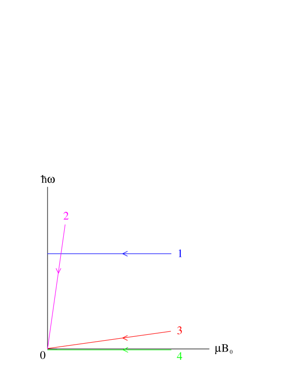
where $B_{0},B_{z}$ and $\mu$ are constants. The case $B_{z}\neq 0$ corresponds to the model without level crossing discussed above, and the geometric phase becomes trivial for $B_{0}\rightarrow 0$.

Fig. 1: The path 1 for $(y_{1},y_{2},y_{3})=(B_{0}\cos\omega t,B_{0}\sin\omega t,0)$ gives rise to the phase change rule (namely, $\cos\theta=0$ in (3.12)) for a fixed finite $T=2\pi/\omega$ and $\mu B_{0}/\hbar\omega\gg 1$, whereas the path 2 gives a trivial phase for a fixed finite $T$ and $\mu B_{0}/\hbar\omega\ll 1$, thus resulting in the failure of the topological argument for the phase change rule for any fixed finite $T$.

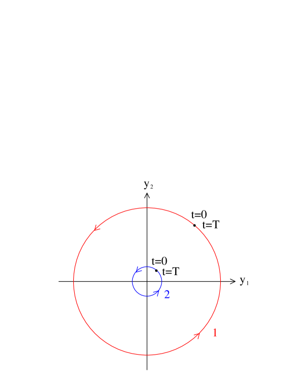
The case $B_{z}=0$ and $B_{0}\rightarrow 0$ describes a cyclic evolution in the infinitesimal neighborhood of level crossing, and the geometric phase becomes trivial if $T=2\pi/\omega$ is kept fixed. On the other hand, the usual adiabatic approximation (with $\theta=\pi/2$ in the present model) in the neighborhood of level crossing is described by $B_{z}=0$ and $B_{0}\rightarrow 0$ (and $\omega\rightarrow 0$) with

$$\mu B_{0}/\hbar\omega\gg 1$$ (4.5)

kept fixed, namely, the ”effective magnetic field” is always strong; the topological proof of phase-change rule [6] (namely, $\cos\theta=0$ in (3.12)) is based on the consideration of this case. It should be noted that the geometric phase becomes trivial for $B_{0}\rightarrow 0$ with $B_{z}=0$ and

$$\mu B_{0}/\hbar\omega\ll 1$$ (4.6)

kept fixed. (If one starts with $B_{z}=0$ and $\omega=0$, of course, no geometric terms.) It is clear that the topology is non-trivial only for a quite narrow (essentially measure zero) window of the parameter space $(B_{0},\omega)$ in the approach to the level crossing $B_{0}\rightarrow 0$.

Fig. 2: Summary of the behavior of the geometric phases in the approach to the level crossing point $B_{0}\rightarrow 0$ in the parameter space $(\mu B_{0},\hbar\omega)$. The path 1 with fixed $\omega=2\pi/T\neq 0$ and also the path 2 with fixed $\mu B_{0}/\hbar\omega\ll 1$ give a trivial phase for $B_{0}\rightarrow 0$. The path 3 with fixed $\mu B_{0}/\hbar\omega\gg 1$ gives a non-trivial phase for $B_{0}\rightarrow 0$. The path 4 with $\omega=0$ gives no geometric phase. The non-trivial phase arises for an essentially measure zero set in the parameter space $(\mu B_{0},\hbar\omega)$ for the approach to the level crossing $B_{0}\rightarrow 0$.

The path integral, where the Hamiltonian is diagonalized both at $t=0$ and $t=T$ if $X(T)=X(0)$,

$$Z = \int\prod_{n}{\cal D}a_{n}^{\star}{\cal D}a_{n}\exp\{\frac{i}{\hbar}\int_{0}^{T}dt[\sum_{n}a_{n}^{\star}(t)i\hbar\frac{\partial}{\partial t}a_{n}(t)$$ (4.7)

$$-\sum_{n,m}a_{n}^{\star}(t)E_{nm}(X(t))a_{m}(t)]\}$$

shows no obvious singular behavior at the level crossing point. On the other hand, the path integral with $\{v_{n}(\vec{x},X(t))\}$ in (2.8) is subtle at the level crossing point; the bases $\{v_{n}(\vec{x},X(t))\}$ are singular on top of level crossing as is seen in (3.5), and thus the induced geometric terms become singular in

$$Z=\int\prod_{n}{\cal D}b_{n}^{\star}{\cal D}b_{n}\exp\{\frac{i}{\hbar}\int_{0}^{T}dt[\sum_{n}b_{n}^{\star}(t)i\hbar\frac{\partial}{\partial t}b_{n}(t)$$

$$+\sum_{n,m}b_{n}^{\star}(t)\langle n|i\hbar\frac{\partial}{\partial t}|m\rangle b_{m}(t)-\sum_{n}b_{n}^{\star}(t){\cal E}_{n}(X(t))b_{n}(t)]\}.$$ (4.8)

The present analysis, however, shows that the path integral is not singular for any finite $T$ if one chooses a suitable regular basis near the level crossing point. We consider that this result is natural since the starting Hamiltonian (3.1) does not contain any obvious singularity.

5 Discussion

The notion of Berry’s phase is known to be useful in various physical contexts [18, 19], and the topological considerations are often crucial to obtain a qualitative understanding of what is going on. Our analysis [16, 17] however shows that the geometric phase associated with level crossing becomes topologically trivial in practical physical settings with any finite $T$. This is in sharp contrast to the Aharonov-Bohm phase which is induced by the time-independent gauge potential and topologically exact for any finite time interval $T$. The fact that the geometric phase becomes topologically trivial for practical physical settings with any fixed finite $T$, such as in the practical Born-Oppenheimer approximation where a large but finite ratio of two time scales is involved and $T$ is identified with the period of the slower system, has not been clearly stated in the literature. We emphasize that this fact is proved independently of the adiabatic approximation.

Our analysis shows that the notion of the geometric phase is useful, but great care needs to be exercised as to its topological properties. From the present point of view, the essence of geometric phases is contained in (2.12): If one evaluates the right-hand side one obtains an exact result, but the physical picture of what is going on is not clear. On the other hand, if one makes an approximation (adiabatic approximation) on the left-hand side of (2.12), one obtains a clear physical picture though the result becomes inevitably approximate.

As for the technical aspect of the present approach, it has been recently emphasized [20] that the notion of hidden local gauge symmetry plays a central role in the actual analyses instead of the notions of parallel transport and holonomy.

References

- [1] S. Pancharatnam, Proc. Indian Acad. Sci. A44, 247 (1956), reprinted in Collected Works of S. Pancharatnam, (Oxford University Press, 1975).
- [2] S. Ramaseshan and R. Nityananda, Curr. Sci. 55, 1225 (1986).
- [3] M.V. Berry, J. Mod. Optics 34, 1401 (1987).
- [4] M.V. Berry, Proc. Roy. Soc. A392, 45 (1984).
- [5] B. Simon, Phys. Rev. Lett. 51, 2167 (1983).
- [6] A.J. Stone, Proc. Roy. Soc. A351, 141 (1976).
- [7] H. Longuet-Higgins, Proc. Roy. Soc. A344, 147 (1975).
- [8] F. Wilczek and A. Zee, Phys. Rev. Lett. 52, 2111 (1984).
- [9] H. Kuratsuji and S. Iida, Prog. Theor. Phys. 74, 439 (1985).
- [10] J. Anandan and L. Stodolsky, Phys. Rev. D35, 2597 (1987).
- [11] Y. Aharonov and J. Anandan, Phys. Rev. Lett. 58, 1593 (1987).
- [12] M.V. Berry, Proc. Roy. Soc. A414, 31 (1987).
- [13] J. Samuel and R. Bhandari, Phys. Rev. Lett. 60, 2339 (1988).
- [14] Y. Lyanda-Geller, Phys. Rev. Lett. 71, 657 (1993).
- [15] R. Bhandari, Phys. Rev. Lett. 88, 100403 (2002).
- [16] K. Fujikawa, Mod. Phys. Lett. A20, 335 (2005), quant-ph/0411006.
- [17] S. Deguchi and K. Fujikawa, ”Second quantized formulation of geometric phases” (to appear in Phys. Rev. A), hep-th/0501166.
- [18] A. Shapere and F. Wilczek, ed., Geometric Phases in Physics (World Scientific, Singapore, 1989).
- [19] D. Chruscinski and A. Jamiolkowski, Geometric Phases in Classical and Quantum Mechanics (Birkhauser, Berlin, 2004).
- [20] K. Fujikawa, ”Geometric phases and hidden local gauge symmetry”, (to appear in Phys. Rev. D), hep-th/0505087.