SISSA/49/2005/EP

Singularities and closed time-like curves
in type IIB 1/2 BPS geometries

S.I.S.S.A. Scuola Internazionale Superiore di Studi Avanzati

Via Beirut 4, 34014 Trieste, Italy

INFN, Sezione di Trieste

Abstract

We study in detail the moduli space of solutions discovered in LLM relaxing the constraint that guarantees the absence of singularities. The solutions fall into three classes, non-singular, null-singular and time machines with a time-like naked singularity. We study the general features of these metrics and prove that there are actually just two generic classes of space-times - those with null singularities are in the same class as the non-singular metrics. $AdS/CFT$ seems to provide a dual description only for the first of these two types of space-time in terms of a unitary $CFT$ indicating the possible existence of a chronology protection mechanism for this class of geometries.

1 Introduction

In [1] a class of type IIB 1/2 BPS solutions has been constructed together with their $CFT$ duals. This construction has inspired interesting work in various directions, [2, 3, 4, 5, 6, 7, 8, 9, 10, 11] and [12, 13, 14]. The basic trick of [1] is to note that assuming a certain amount of symmetry in the ansatz for metric and five-form field strength, and demanding that the geometry has a Killing spinor, the remaining equations of motions reduce to an elliptic equation for a scalar function $z$ on $\mathbb{R}^{2}\times\mathbb{R}^{+}$. The value of $\rho=1/2-z$ on the 2-plane boundary of $\mathbb{R}^{2}\times\mathbb{R}^{+}$ can be interpreted as a semiclassical fermion density, thus providing direct contact to the $CFT$ dual Yang-Mills theory on $\mathbb{R}\times S^{3}$[15, 16]. Indeed if this density takes on only the values 0 and 1 then the solutions are guaranteed to be singularity free space-times.

In this paper we consider the most general allowed (on the supergravity side) boundary conditions for the elliptic equation. This means that we study the full set of moduli of this sector of supergravity that consists of metrics asymptotic to $AdS_{5}\times S^{5}$, with an $SO(4)\times SO(4)$ isometry group and preserving half of the supersymmetry of type IIB string theory. The supergravity solutions in general will be singular. The spacetime singularities appearing are always naked and fall into two distinct classes: null and timelike. The null ones can be considered as seeded by a fermion density between 0 and 1 and are already considered in the literature, see for example [17, 18, 19, 20, 21] together with the possible local quantum effects responsible for their resolution - the singularity is due to an average over configurations of $N$ fermions in a gas with average density less than one. An individual configuration with the same asymptotics can actually be seen to have as source a collection of $N$ giant gravitons [22, 23] separated one from the other. In the supergravity theory, the resolution of the singularity thus appears as a sort of space-time foam [24] while in the dual $CFT$ one sees that such a configuration corresponds to the Coulomb branch of the theory.

The $AdS/CFT$ correspondence has maybe something more interesting to tell us about the fate of the timelike singularities. The solutions with this kind of singularity are highly “pathological”: they have closed timelike curves passing through any point of the spacetime and they include unbounded from below negative mass excitations of $AdS_{5}\times S^{5}$.

It has already been conjectured, [25, 26, 27], that geometries with these features should be considered as truly unphysical via global considerations in the setting of a full quantum theory of gravity. The $AdS/CFT$ correspondence applied to the space-times of [1] suggests one particular mechanism for the global removal of solutions containing timelike singularities. The deformations of the geometry which produce these singularities apparently correspond to negative dimension operators in the dual field theory. The unitarity of the representations of the superalgebra $SU(2,2|4)$ [28] indicate in particular that unitary operators must have a positive conformal dimension. Our observations indicate that there should actually exist a general proof of the chronology protection conjecture [29] in this sector of supergravity . A first indication of this mechanism linking unitarity to chronology protection can be found in [30] and in the current context in [31, 32].

Extending these works, in this paper we prove that closed timelike curves (CTCs) are unavoidable in any solution with a timelike singularity and that they are excluded in the case of regular and null singular solutions, these being the spacetimes that can be represented in terms of dual fermions, a result anticipated but not proven in [31]. This provides a clear division between these two classes of singular spacetimes which is also reflected in the two different mechanisms responsible for the resolution of their respective spacetime singularities.

In Section 2 we review the construction of [1] and we show the most general allowed boundary conditions for a supergravity solution satisfying the symmetry requirements. We clarify the role of the boundary conditions in determining the radius of the asymptotic $AdS_{5}\times S^{5}$ and we show the relation between the boundary conditions and the appearance of spacetime singularities.

In Section 3 we exhibit some examples of singular supergravity solutions and we uncover some of their properties such as CTCs and peculiar geometric features. In particular we exhibit unbounded from below (for fixed $AdS$ radius) negative mass excitations of $AdS_{5}\times S^{5}$.

In Section 4 we show that most of the interesting features of the examples in Section 3, regarding mainly the appearance and the properties of CTCs, are generic for the case of solutions with timelike singularities. Moreover we prove a theorem which clearly relates the appearance of CTCs to the boundary conditions responsible for timelike singularities.

In section 5 we return to a discussion of the meaning of these results, and in particular the possibility of proving the chronology protection conjecture for this class of geometries, by showing that the $AdS/CFT$ correspondence relates naked time machines to non-unitarity in the $CFT$.

In the Appendix we show that there is just one plane wave geometry, the maximally supersymmetric one of [33], that can be obtained from the construction presented in [1].

2 LLM construction

In the first part of this section we review the construction of [1] in a language adapted to the considerations that follow in the rest of this paper.

In [1] a class of BPS solutions of type IIB supergravity is constructed. This is the most general class of BPS solutions in type IIB supergravity with $SO(4)\times SO(4)$ isometry, one timelike Killing vector and a non-trivial self-dual 5-form field strength $F_{(5)}$. The solutions are given by

$$\mathrm{d}s^{2}=-h^{-2}(\mathrm{d}t+V_{i}\mathrm{d}x^{i})^{2}+h^{2}(\mathrm{d}y^{2}+\delta_{ij}\mathrm{d}x^{i}\mathrm{d}x^{j})+y\mathrm{e}^{G}\mathrm{d}\Omega_{3}^{2}+y\mathrm{e}^{-G}\mathrm{d}\mathaccent 869{\Omega}_{3}^{2}$$ (2.1)

$$F_{(5)}=F_{\mu\nu}\mathrm{d}x^{\mu}\wedge\mathrm{d}x^{\nu}\wedge\mathrm{d}\Omega+\mathaccent 869{F}_{\mu\nu}\mathrm{d}x^{\mu}\wedge\mathrm{d}x^{\nu}\wedge\mathrm{d}\mathaccent 869{\Omega}$$ (2.2)

$$F=\mathrm{e}^{3G}\ast_{4}\mathaccent 869{F}$$ (2.3)

with $y\geq 0$.
We can define a function $z=z(x_{1},x_{2},y)$ which determines the entire solution (up to choice of gauge that we discuss below),

$$z\equiv\frac{1}{2}\tanh G$$ (2.5)

$$h^{-2}=2y\cosh G=\frac{y}{\sqrt{(1/2-z)(1/2+z)}}$$ (2.6)

$$\mathrm{d}V=\frac{1}{y}\ast_{3}\mathrm{d}z$$ (2.7)

$$F=\mathrm{d}(B_{t}(\mathrm{d}t+V))+\mathrm{d}\hat{B}$$ (2.8)

$$\tilde{F}=\mathrm{d}(\tilde{B}_{t}(\mathrm{d}t+V))+\mathrm{d}\hat{\tilde{B}}$$ (2.9)

$$B_{t}=-\frac{1}{4}y^{2}\mathrm{e}^{2G}\qquad\tilde{B}_{t}=-\frac{1}{4}y^{2}\mathrm{e}^{-2G}$$ (2.10)

$$\mathrm{d}\hat{B}=-\frac{1}{4}y^{3}\ast_{3}\mathrm{d}\left(\frac{1/2+z}{y^{2}}\right)\qquad\mathrm{d}\hat{\tilde{B}}=\frac{1}{4}y^{3}\ast_{3}\mathrm{d}\left(\frac{1/2-z}{y^{2}}\right)$$ (2.11)

where $\ast_{n}$ indicate the Hodge dual in $n$ flat dimensions.
For the consistency of (2.7) we must have

$$(\partial_{1}^{2}+\partial_{2}^{2})z+y\partial_{y}(\frac{1}{y}\partial_{y}z)=0$$ (2.12)

The solutions for $z$ are determined by boundary conditions in the $\{x_{1},x_{2},y\}$ space as we will now discuss.

2.1 Boundary conditions

The solution is well defined for $z$ restricted to the range

$$-1/2\leq z\leq 1/2$$ (2.13)

Equation (2.12) implies that $z$ takes its maximum and minimum on the boundary of its domain of definition $\Sigma\subset\mathbb{R}^{2}\times\mathbb{R}^{+}$. A solution of the supergravity equations is thus specified by a choice of $\Sigma$, and by a function $z_{0}$ defined on $\partial\Sigma$ such that

$$z=z_{0}\qquad\text{on}\,\,\partial\Sigma$$ (2.15)

$$-1/2\leq z_{0}\leq 1/2$$

Following [1] one can easily show that if $\Sigma$ extends to infinity and $z$ goes to either $1/2$ or $-1/2$ for $r^{2}=x_{1}^{2}+x_{2}^{2}+y^{2}\rightarrow\infty$, the solution is asymptotically $AdS_{5}\times S^{5}$. Changing $z$ into $-z$ is a symmetry of the solution and thus we assume for definiteness

$$z\rightarrow\frac{1}{2}\,\,\text{for}\,\,r^{2}=x_{1}^{2}+x_{2}^{2}+y^{2}\rightarrow\infty$$ (2.16)

We call $\partial\Sigma_{0}$ the intersection of $\partial\Sigma$ with the $y=0$ plane, and $\partial\hat{\Sigma}=\partial\Sigma\setminus\partial\Sigma_{0}$. We note that if $z_{0}\neq\pm\frac{1}{2}$ on $\partial\hat{\Sigma}$ then the metric can be analytically continued as far as $y=0$ or $z=\pm\frac{1}{2}$. In general, after analytically continuing the solution, we have a larger “maximal” domain $\Sigma^{\prime}\supset\Sigma$ where $-\frac{1}{2}\leq z\leq\frac{1}{2}$.

For convenience we will call again $\Sigma$ this maximal domain of definition. The most general asymptotically $AdS_{5}\times S^{5}$ solution of the supergravity equations is then specified by the domain ${\Sigma}$ and a function $z_{0}$ on $\partial\Sigma$

$$\begin{cases}-\frac{1}{2}\leq z_{0}\leq\frac{1}{2}\quad&\text{on}\,\,\partial\Sigma_{0}\\ z_{0}=\pm\frac{1}{2}\quad&\text{on}\,\,\partial\hat{\Sigma}\\ z_{0}\rightarrow\frac{1}{2}\quad&\text{for}\,\,r\rightarrow\infty\end{cases}$$ (2.17)

as illustrated in Figure 1.

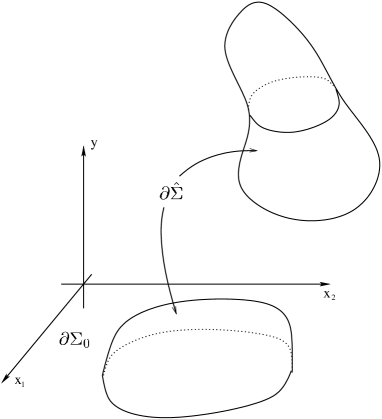
Figure 1: The domain of definition $\Sigma$

We define a new function $\Phi$

$$\Phi\equiv\frac{\frac{1}{2}-z}{y^{2}}$$ (2.18)

The equation for $z$ is equivalent to the Laplace equation for $\Phi$ on a flat six dimensional space of the form $\mathbb{R}^{2}\times\mathbb{R}^{4}$ where $x_{1},x_{2}$ are the coordinates on the $\mathbb{R}^{2}$ and $y$ is the radius for spherical coordinate on the $\mathbb{R}^{4}$. Since (2.12) and the definition of $\Phi$ are singular for $y=0$, Dirichlet boundary conditions for $z$ on $y=0$ take the role of charge sources for $\Phi$ located at $y=0$. Thus $\Phi$ satisfies the equation

$$\left\{\begin{split}&(\partial_{1}^{2}+\partial_{2}^{2})\Phi+\frac{1}{y^{3}}\partial_{y}(y^{3}\partial_{y}\Phi)=\ast_{6}\mathrm{d}\ast_{6}\mathrm{d}\Phi=-4\pi^{2}(\frac{1}{2}-z_{0})\delta^{(4)}(y)\chi(\Sigma_{0})\\ &\Phi=\frac{\frac{1}{2}-z_{0}}{y^{2}}\,\,\text{on}\,\partial\hat{\Sigma}\end{split}\right.$$ (2.19)

where

$$\chi(\Sigma_{0})(x_{1},x_{2})=\begin{cases}1&\text{if}\,\,(x_{1},x_{2})\in\Sigma_{0}\\ 0&\text{otherwise}\end{cases}.$$ (2.20)

The forms $B,\tilde{B}$ and $V$ are defined up to a gauge transformation. From now on we will use the following convenient gauge for $V$

$$\mathrm{d}\ast_{3}V=0\iff\partial_{1}V_{1}+\partial_{2}V_{2}=0$$ (2.21)

2.2 Asymptotic behaviour

The boundary conditions (2.17) imply that

$$\Phi\rightarrow\frac{A}{(x_{1}^{2}+x_{2}^{2}+y^{2})^{2}}=\frac{A}{r^{4}},\qquad r\rightarrow\infty,\qquad A>0.$$ (2.22)

Integrating (LABEL:laplace_for_phi) we obtain

$$A\,4\pi^{3}=\int_{S^{5}(r)}(-\ast_{6}\mathrm{d}\Phi)=\int_{\hat{\Sigma}^{5}}(-\ast_{6}\mathrm{d}\Phi)+4\pi^{2}\int_{\partial\Sigma_{0}}\left(\frac{1}{2}-z_{0}(x_{1},x_{2})\right)\mathrm{d}x_{1}\mathrm{d}x_{2}$$ (2.23)

where $S^{5}(r)$ is a 5-sphere of radius $r$ centered on the origin, and $\hat{\Sigma}^{5}$ is the 5-manifold obtained by the fibration in spherical coordinates of a 3-sphere $S^{3}(y)$ over $\partial\hat{\Sigma}$.
Going to polar coordinates $R,\varphi$ in the $\{x_{1},x_{2}\}$ sections and for $R^{2}+y^{2}\rightarrow\infty$, $V$ has the asymptotic behaviour

$$V\approx V_{\varphi}\mathrm{d}\varphi\qquad V_{\varphi}\approx-A\frac{R^{2}}{(R^{2}+y^{2})^{2}}.$$ (2.24)

In [1] it has been shown that the quantity $A$ determines the radius of the asymptotic $AdS_{5}\times S^{5}$

$$R^{2}_{AdS_{5}}=R^{2}_{S^{5}}=A^{1/2}$$ (2.25)

In the asymptotic region we can construct a smooth five dimensional manifold $\tilde{\Lambda}_{5}$ by fibering the three sphere $\tilde{S}^{3}$ over a surface $\tilde{\Lambda}_{2}$.
The topology of $\tilde{\Lambda}_{5}$ is asymptotically $S^{5}$. The flux of the five form through this surface is given by

$$N=-\frac{1}{4\pi^{4}l_{P}^{4}}\int_{\tilde{\Lambda}_{5}}\mathrm{d}\hat{\tilde{B}}\wedge\mathrm{d}\tilde{\Omega}_{3}=-\frac{1}{16\pi^{4}l_{P}^{4}}\int_{\tilde{\Lambda}_{5}}\ast_{6}\mathrm{d}\Phi=\frac{1}{4\pi l_{P}^{4}}A=\frac{1}{4\pi l_{P}^{4}}R_{AdS_{5}}^{4}$$ (2.26)

which agrees with the standard formula for the relation between the radius of $AdS_{5}$ and the flux of $F_{(5)}$.

The mass of the excitation of $AdS_{5}\times S^{5}$ can be computed by looking at subleading terms in the expansion of $\Phi$ around $r\rightarrow\infty$.

2.3 Regular solutions and dual picture

If we choose $\Sigma=\mathbb{R}^{2}\times\mathbb{R}^{+}$ the solution can be written as

$$z=\frac{1}{2}-\Phi\,y^{2}=\frac{1}{2}-\frac{y^{2}}{\pi}\int\frac{\rho(x_{1}^{\prime},x_{2}^{\prime})\mathrm{d}^{2}x^{\prime}}{[(x_{1}-x_{1}^{\prime})^{2}+(x_{2}-x_{2}^{\prime})^{2}+y^{2}]^{2}}$$ (2.27)

$$V_{i}=-\frac{1}{\pi}\epsilon_{ij}\int\frac{(x_{j}-x_{j}^{\prime})\rho(x_{1}^{\prime},x_{2}^{\prime})\mathrm{d}^{2}x^{\prime}}{[(x_{1}-x_{1}^{\prime})^{2}+(x_{2}-x_{2}^{\prime})^{2}+y^{2}]^{2}}$$ (2.28)

with

$$\rho(x_{1},x_{2})=\frac{1}{2}-z_{0}(x_{1},x_{2})$$ (2.29)

According to [1], in the dual field theory these excitation of $AdS_{5}\times S^{5}$ are described by $N$ free fermions. The plane $y=0$ can be identified with the phase space of the dual fermions and the function $\rho(x_{1},x_{2})$ can be identified with the semiclassical density of these fermions.

It can be shown that the metric is regular if $\Sigma=\mathbb{R}^{2}\times\mathbb{R}^{+}$ and $z_{0}$ takes the values $\pm 1/2$ on the $y=0$ plane [1]. In these cases $\rho$ is non vanishing just inside the “droplets” where $z_{0}=-1/2$

$$\rho=\begin{cases}\beta=1\,&\text{inside the droplets}\\ 0\,&\text{outside}\end{cases}$$ (2.30)

Since we have assumed that $z\rightarrow 1/2$ at infinity, we can always find a circle large enough to encircle all “droplets”. With these boundary conditions $z$ is given by

$$z=\frac{1}{2}-\frac{y^{2}}{\pi}\int_{\mathcal{D}}\frac{\mathrm{d}^{2}x^{\prime}}{[(x_{1}-x_{1}^{\prime})^{2}+(x_{2}-x_{2}^{\prime})^{2}+y^{2}]^{2}}$$ (2.31)

$\mathcal{D}$ being the union of the droplets where $z=-1/2$. The $V$ form can be written

$$V_{i}=-\frac{1}{\pi}\epsilon_{ij}\int_{\mathcal{D}}\frac{(x_{j}-x_{j}^{\prime})\mathrm{d}^{2}x^{\prime}}{[(x_{1}-x_{1}^{\prime})^{2}+(x_{2}-x_{2}^{\prime})^{2}+y^{2}]^{2}}$$ (2.32)

The determinant of the sections $\{x_{1},x_{2},y\}$ is given by

$$\tilde{g}=h^{4}-V_{1}^{2}-V_{2}^{2}=\frac{1/4-z^{2}}{y^{2}}-V^{2}$$ (2.33)

Note that here and in the following $V^{2}$ is formed by contracting indices using the Kronecker delta, i.e. $V^{2}\equiv V_{1}^{2}+V^{2}_{2}$. Theorem 4.1 of Section 4 states that for any $\mathcal{D}$, $\tilde{g}\geq 0$ and the $\{x_{1},x_{2},y\}$ sections do not contain time-like directions. This guarantees in particular that the original LLM solutions are free of CTCs and are “good” supergravity solutions.

From the analysis of Section 2.2, we can deduce that the radius of the asymptotic $AdS_{5}\times S^{5}$ is given by

$$R_{AdS}^{4}=\frac{\mathcal{S}}{\pi}=A$$ (2.34)

where

$$\mathcal{S}=\int_{\mathcal{D}}\mathrm{d}x_{1}\mathrm{d}x_{2}$$ (2.35)

is the total area of all droplets where $z=-\frac{1}{2}$ ($\rho=1$). The quantization of the flux (2.26) gives the quantization condition on the area of the droplets

$$\mathcal{S}=4\pi^{2}l_{p}^{4}N$$ (2.36)

If $\mathcal{D}$ consists of one single circular droplet then the spacetime is precisely $AdS_{5}\times S^{5}$. For a generic set of droplets $\mathcal{D}$ the mass (and the angular momentum) of the excitation is given by

$$M=J=\frac{1}{8\pi^{2}l_{P}^{8}}\left[\frac{1}{2\pi}\int_{\mathcal{D}}(x_{1}^{2}+x_{2}^{2})\mathrm{d}^{2}x-\left(\frac{1}{2\pi}\int_{\mathcal{D}}\mathrm{d}^{2}x\right)^{2}\right]\geq 0$$ (2.37)

The origin of the coordinates is chosen such that the dipole vanishes, that is,

$$\int_{\mathcal{D}}x_{i}\mathrm{d}^{2}x=0.$$ (2.38)

Not surprisingly one can show by a direct calculation that the equality ($M=J=0$) holds for a single disk. Given any $\mathcal{D}$ we can build a disk $C_{\mathcal{D}}$ of the same area. The first term is clearly larger for $\mathcal{D}$ than for $C_{\mathcal{D}}$ and thus in general $M>0$ for the non-singular solutions.

2.4 More general boundary conditions and singularities

In all cases with boundary conditions different from the ones studied in [1] we have spacetime singularities.

It is easy to see that the solutions have a naked time-like singularity when $\partial\hat{\Sigma}$ is non-empty. Consider a surface in the region $y>0$ on which $z=-1/2$ (the discussion does not change in any substantial way if instead we took $z=1/2$). Choose a point $Q$ on this surface and define a coordinate $\epsilon$ in the $\{x_{1},x_{2},y\}$ space orthogonal to this surface such that $z=-1/2+\alpha\epsilon$ for some positive constant $\alpha$. Complete $\epsilon$ to a new orthogonal coordinate system by introducing two coordinates $v_{i}$ with origin at $Q$. This is just an orthogonal transformation and translation of the original coordinate system. At $Q$ we can assume that $V$ is finite with a power series expansion away from this point. The subleading terms in this expansion are not important for studying the singularity. We also define a new time coordinate near Q by $T=t+V_{i}(Q)x_{i}$. Keeping just the leading divergences and introducing $\rho=(\alpha\epsilon)^{5/4}$ the metric expanded around $Q$ is

$$\mathrm{d}s^{2}=\alpha\rho^{-2/5}(-\mathrm{d}T^{2}+\mathrm{d}\tilde{\Omega}_{3}^{2})+\frac{16}{25}\mathrm{d}\rho^{2}+\rho^{2/5}(\mathrm{d}v_{i}^{2}+\mathrm{d}\Omega_{3}^{2}).$$ (2.39)

A short calculation then shows that the metric is singular with scalar curvature as $\rho\rightarrow 0$

$$R=-\frac{5}{16\rho^{2}}$$ (2.40)

and the singularity is clearly time-like with no horizon.

Singularities are located also on the subset of $\partial\Sigma_{0}$ where $z\neq\pm\frac{1}{2}$. All these singularities are naked and null.

Indeed assuming that $1/4-z^{2}\rightarrow\alpha^{2}$ as $y\rightarrow 0$ and looking at the $\{t,y\}$ sections we find

$$\mathrm{d}s^{2}=-\alpha^{-1}\,y\,\mathrm{d}t^{2}+\alpha\,y^{-1}\,\mathrm{d}y.$$ (2.41)

With the change of variables, $u=\sqrt{y/\alpha}\,\mathrm{e}^{-t/2}$ $v=\sqrt{y/\alpha}\,\mathrm{e}^{t/2}$, the metric becomes simply

$$\mathrm{d}s^{2}=\mathrm{d}u\mathrm{d}v$$ (2.42)

and the singularity is along the curves, $u=0$ and $v=0$. The singularity is due to the way in which the radii of the two three spheres, $S^{3}$ and $\tilde{S}^{3}$ go to zero [17].

3 Singular solutions: some examples

Interpreting $\rho=1/2-z_{0}$ as the density of the dual fermions, one first natural generalization of the boundary conditions in [1] is to have density $\rho\neq 1$. We note that for generic $\rho(x_{1},x_{2})$, the radius of the asymptotic $AdS_{5}\times S^{5}$ is given by

$$R_{AdS}^{4}=\frac{1}{\pi}\int\rho(x_{1},x_{2})\mathrm{d}^{2}x$$ (3.1)

We have that $0\leq\rho\leq 1$ (that is $-1/2\leq z_{0}\leq 1/2$), if and only if $\partial\hat{\Sigma}=\emptyset$. In this case all the singularities will be null.

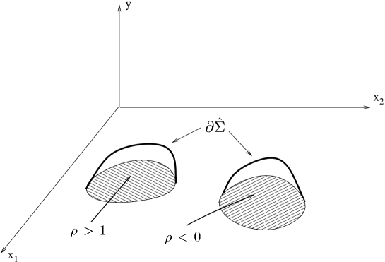
Figure 2: Two regions of $y=0$ plane, one with $\rho>1$ and the other with $\rho<0$, leading to a non trivial $\partial\hat{\Sigma}$ attached to the $y=0$ plane

The mass of the excitation is now given by

$$M=\frac{1}{8\pi^{2}l_{P}^{8}}\left[\frac{1}{2\pi}\int\rho(x_{1},x_{2})(x_{1}^{2}+x_{2}^{2})\mathrm{d}^{2}x-\left(\frac{1}{2\pi}\int\rho(x_{1},x_{2})\mathrm{d}^{2}x\right)^{2}\right]$$ (3.2)

with origin chosen again in such a way that the dipole vanishes

$$\int_{\mathcal{D}}\rho(x_{1},x_{2})x_{i}\mathrm{d}^{2}x=0.$$ (3.3)

We note that for fixed value of $R_{AdS}$ there is a lower bound on the mass obtained for $\rho=\pi R_{AdS}^{4}\delta^{(2)}(x_{1},x_{2})$,

$$M_{\text{min}}=-\frac{R_{AdS}^{8}}{32\pi^{2}l_{P}^{8}}$$ (3.4)

A priori we can consider also $\rho(x_{1},x_{2})<0$ in some domains provided that the integral defining $R_{AdS}^{4}$ remains positive. One can easily see that the cases $\rho>1$ and $\rho<0$ correspond to choosing a $\partial\hat{\Sigma}$ not empty and attached to the $y=0$ plane, as in Figure 2. Taking $\rho$ negative in some region we can easily obtain arbitrary large negative value of the mass for fixed $R_{AdS}$. It’s enough to have $\rho<0$ even in a very small region provided it is located at large $x_{1}^{2}+x_{2}^{2}$. In the next subsections we will restrict to the case $\rho\geq 0$, studying some examples with features that will serve as a guide for the general analysis of Section 4.

The appearance of CTCs, which we will show to be unavoidable in Section 4, and unbounded from below negative mass values suggest that one should consider as unphysical the geometries seeded by a density $\rho$ that does not remain between 0 and 1. For the sake of causality and for the stability of the quantum version of the supergravity theory, these solutions should be regarded as unphysical on the basis of some global argument. If the singularity was resolved by quantum effects through some local mechanism and “smoothed”, then the asymptotics and mass could not change significantly; moreover, we know that the existence of CTCs is a manifestation of global properties of the spacetime. Before discussing the possibility of such a resolution we will study these singular geometries in more detail.

For simplicity, we will first study the case of piecewise constant $\rho$. Assuming $\rho=\sum_{i}\beta_{i}\chi(\mathcal{D}_{i})$ the $z$ function can be written as

$$z=1/2-\frac{y^{2}}{\pi}\sum_{i}\beta_{i}\int_{\mathcal{D}_{i}}\frac{\mathrm{d}^{2}x^{\prime}}{[(x_{1}-x_{1}^{\prime})^{2}+(x_{2}-x_{2}^{\prime})^{2}+y^{2}]^{2}}$$ (3.5)

The solution seeded by these density distributions can have null singularities or naked time machines. Solutions with null singularities are already discussed in the literature in various places [17, 18, 19, 20, 21] although we have some additional interesting observations to make. These issues will be discussed in section 3.1. In section 3.2 and 3.3 we will discuss the general features of configurations with naked timelike singularities, in particular illustrating a novel geometric mechanism for producing CTCs. In Section 3.4 we study the specific case of the geometry seeded by a circular droplet of density $\beta>1$.

In Section 3.5 we discuss a class of solutions which does not have a density distribution $\rho(x_{1},x_{2})$ in the $y=0$ plane as source, but rather appears as a natural continuation of the solutions studied in 3.4. These solutions are indeed determined by a $\partial\hat{\Sigma}$ which does not intersect the $y=0$ plane. They exhibit CTCs and their mass is unbounded from below. Any possible direct connection to the free fermion picture is lost.

3.1 $\beta_{i}\leq 1$ with at least one $\beta_{i}<1$

This case was already briefly considered in [1]. These geometries have null singularities located on the $y=0$ plane inside the droplets. We will show in Section 4.3 that also these geometries are free of CTCs.

It is straightforward to show that if $\beta_{i}\leq 1$ the mass given by (3.2) is always nonnegative. These configurations can be viewed as an averaged version of a dilute gas of fermions. In this case one can think that the singularity is resolved by local quantum effects by the appearance of a “spacetime foam” [24] and in the dual theory by simply moving to the Coulomb branch of the moduli space.

Geometries corresponding to a single circular droplet of density $\beta<1$ are precisely the solutions considered in [17].

In the limit that the radius goes to infinity, this describes the $N\rightarrow\infty$ limit of the Coulomb branch in the dual gauge theory, as amply discussed in [1]. The corresponding classical geometry is singular but is regularized as above by the dilute fermi gas, or in geometric language, a dilute gas of giant gravitons, the geometry of which is clearly smooth.

This solution leads one to an interesting relation between a limit of the dual SCFT and the singular homogeneous plane wave metrics that arise generically as the Penrose limit of “reasonable” space-time singularities [34].

For simplicity one can actually consider the boundary condition $\rho=\beta<1$ for all $(x_{1},x_{2})$. Consider a null geodesic that ends on the “null” singularity and take the Penrose Limit with respect to this null geodesic.

In such a case it is easy to see that the resulting metric is exactly,

$$\mathrm{d}s^{2}=2\mathrm{d}u\mathrm{d}v+(3(x_{1}^{2}+x_{2}^{2})-\sum_{i=1}^{6}w_{i}^{2})\frac{\mathrm{d}u^{2}}{u^{2}}+\mathrm{d}x^{2}+\mathrm{d}w^{2}.$$ (3.6)

In principle this provides a SYM dual description of the singular plane waves as a limit (analogous to the BMN [35] limit of AdS/CFT) of the $N\rightarrow\infty$ Coulomb branch in the original dual CFT.

3.2 Some $\beta_{i}>1$

This boundary condition is equivalent to lifting the surface $z=-1/2$ above the $\{x_{1},x_{2}\}$ plane keeping its boundary fixed at $y=0$. The continuation of $z$ inside this surface to $y=0$ will give a non-trivial function everywhere less than $-1/2$. This is the first example of the non-empty $\partial\hat{\Sigma}$ introduced in Section 2.

The emerging geometries have timelike singularities on $\partial\hat{\Sigma}$ and CTCs. They include also negative (but bounded from below) mass excitations of $AdS_{5}\times S^{5}$, as anticipated at the beginning of this section.

In the next subsections we will focus on the $\{x_{1},x_{2},y\}$ sections. They contain almost all of the interesting features.

3.3 Zooming

We consider the leading term of the expansion of $z$ and $V$ for points close to $y=0$ and the boundary of one droplet of constant density $\beta>1$. More precisely, with $L$ the typical dimension of the droplet and $R$ the radius of curvature of the boundary, we assume that $y$ and the distance to the boundary are both much smaller than $L$ and $R$. The leading term can be obtained solving the equations for $z$ with boundary condition

$$\rho(x_{1},x_{2})=\begin{cases}\beta\quad,&x_{2}<0\\ 0\quad,&x_{2}>0\end{cases}$$ (3.7)

The case $\beta=1$ has already been considered in [1] and corresponds to the maximally supersymmetric plane wave [33]. We note here that only in the case of $\beta=1$ the “zooming” limit that we are considering here coincides with the Penrose limit. Indeed the BFHP plane wave is the only plane wave geometry that can be obtained via the LLM construction and its generalization with the most general boundary conditions on $z$ considered in Section 2. All (generalized) LLM metrics, have 16 Killing spinors $\psi$ whose bilinears $\bar{\psi}\Gamma^{M}\psi$ are null Killing vectors but not covariantly constant (c.c.). Any plane wave has 16 Killing spinors with c.c. Killing vector bilinear, and the only one which has 16 extra Killing spinors is the maximally supersymmetric one. The details of the proof can be found in the Appendix.

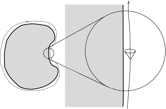
Figure 3: Zoom showing light cone near a droplet with $\beta_{i}>1$ on the $\{x_{1},x_{2}\}$ plane at $y=0$.

For generic $\beta$ we have

$$z=\frac{\beta}{2}\frac{x_{2}}{\sqrt{x_{2}^{2}+y^{2}}}+\frac{1}{2}(1-\beta)=\frac{\beta}{2}\cos\theta+\frac{1}{2}(1-\beta)$$ (3.8)

$$V_{1}=\frac{\beta}{2\sqrt{x_{2}^{2}+y^{2}}}=\frac{\beta}{2R}\qquad V_{2}=0$$ (3.9)

The plane $\cos\theta=\frac{\beta-2}{\beta}$ is $\partial\hat{\Sigma}$ and the domain $\Sigma$ is defined by

$$1>\cos\theta>\frac{\beta-2}{\beta}$$ (3.10)

The vector $\partial_{x_{1}}$ is a Killing vector and

$$g_{11}=\frac{1}{y\sqrt{\rho(1-\rho)}}\left(\frac{\beta}{2}(1-\beta)(1-\cos\theta)\right)<0$$ (3.11)

so that it is timelike. The limit $y\rightarrow 0,\cos\theta\rightarrow 1$ is finite and gives

$$g_{11}\rightarrow(1-\beta)\sqrt{\beta}\frac{1}{2x_{2}}$$ (3.12)

In the same limit, we have

$$g_{22}=h^{2}\rightarrow\frac{\sqrt{\beta}}{2x_{2}}$$ (3.13)

In a neighborhood of $\partial\mathcal{D}$, the $\{x_{1},x_{2}\}$ plane is thus a Lorentz submanifold. We note that the opening of the lightcone is given by

$$\tan\phi=\frac{\mathrm{d}x_{2}}{\mathrm{d}x_{1}}=\pm\sqrt{-\frac{g_{11}}{g_{22}}}=\pm\sqrt{(\beta-1)}$$ (3.14)

From this analysis it is straightforward to conclude that if we have a droplet $\mathcal{D}$ with $\beta_{\mathcal{D}}>1$ of smooth boundary $\partial\mathcal{D}$, provided we stay close enough to the $y=0$ plane and to $\partial\mathcal{D}$ we have CTCs going around $\mathcal{D}$ (Figure 3). Since these geometries have no horizon a CTC passes through any point of the spacetime.

3.4 The disk

It is possible to perform a detailed analysis of the geometry seeded by one single circular droplet of constant density $\beta>1$. The analysis is interesting because it displays some generic features of the timelike singular geometries and it is useful for introducing the more general timelike singularities which we will study in the next section.

We assume that the radius of the droplet is $R_{0}$. The radius of the asymptotic $AdS_{5}\times S^{5}$ is thus given by

$$R_{AdS}^{4}=\frac{1}{\pi}\int\rho=\beta R_{0}^{2}$$ (3.15)

These geometries have already been studied in [31] where it is shown that they can be viewed as a generalisation of the superstar studied in [17]. The superstar geometries are parameterised by a charge $Q$ and a scale parameter $L$, which are related to our $\beta$ and $R_{0}$ in the following way.

$$\beta=\frac{1}{1+Q/L^{2}}\,,\,R_{0}^{2}=L^{2}(L^{2}+Q)\,\Rightarrow\,R_{AdS}=L$$ (3.16)

For fixed value of $L$ we have

$$-L^{2}<Q<0\Rightarrow\beta>1$$ (3.17)

$Q=-L^{2}$ corresponds to $\rho=\pi L^{4}\delta^{(2)}(x_{1},x_{2})$. We will discuss the continuation to $Q<-L^{2}$ in the next section.

Following the analysis in Section 3.3 we expect to find CTCs in these geometries. Going to polar coordinates $R,\varphi$ in the $x_{1},x_{2}$ plane we have

$$z=\frac{\beta}{2}\frac{R^{2}-R_{0}^{2}+y^{2}}{\sqrt{(R^{2}+R_{0}^{2}+y^{2})^{2}-4R^{2}R_{0}^{2}}}+\frac{1}{2}(1-\beta)$$ (3.18)

$$V=V_{\varphi}\mathrm{d}\varphi$$ (3.19)

$$V_{\varphi}=\frac{\beta}{2}\left(1-\frac{R^{2}+R_{0}^{2}+y^{2}}{\sqrt{(R^{2}+R_{0}^{2}+y^{2})^{2}-4R^{2}R_{0}^{2}}}\right)$$ (3.20)

The equation for the $\partial\hat{\Sigma}$ is given by $z=-\frac{1}{2}$

$$R^{2}+\left(y-R_{0}\frac{\beta-2}{2\sqrt{\beta-1}}\right)^{2}-R_{0}^{2}\frac{\beta^{2}}{4(\beta-1)}=0$$ (3.21)

Thus the geometry is defined in the $y\geq 0$ halfspace, outside a sphere of radius $\frac{\beta}{2\sqrt{\beta-1}}R_{0}$ with centre at $R=0$ and $y=\frac{\beta-2}{2\sqrt{\beta-1}}R_{0}$. In particular it crosses the $y$ axis at $y=R_{0}\sqrt{\beta-1}$.

The square of the Killing vector $\partial_{\varphi}$ is

$$g_{\varphi\varphi}=-h^{-2}V_{\varphi}^{2}+R^{2}h^{2}$$ (3.22)

and we have

$$g_{\varphi\varphi}\geq 0\iff\frac{y^{2}}{\beta-1}+\frac{R^{2}}{\beta}-R_{0}^{2}\geq 0.$$ (3.23)

The surface on which $g_{\varphi\varphi}=0$ is known as the velocity of light surface (VLS).

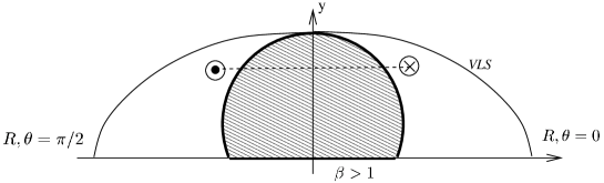
Figure 4: Singularity and velocity of light surface for a disk with $\beta>1$.

From this analysis, three main features follow (see Figure 4). We will show in Section 4.1 that they are generic for geometries seeded by boundary conditions such that $\partial\hat{\Sigma}\neq\emptyset$.

1. The VLS touches the singularity where $V^{2}=0$. If the VLS did not touch the singularity we would have CTCs which are contractible to a point remaining timelike. At such a point the local orientability of spacetime would be lost - possibly indicating also a change in the signature of spacetime to two time-like directions. The fact that the VLS touches the singularity at a point, in such a way that there is no loss of time orientability should be guaranteed, but we know of no general theorem that proves this.

2. The opening of the lightcone in the $\{R,\varphi,y\}$ sections inside the ellipsoid is given by

   $$\tan\theta=\frac{y^{2}}{1/4-z^{2}}V_{\varphi}^{2}-R^{2}$$ (3.24)

   This means that provided we stay close enough to the singularity at $z=-\frac{1}{2}$ and that we go “around” it in the direction indicated by $\partial_{\varphi}$ we have CTCs.

3. All generalized LLM geometries are without horizon and thus a CTC passes through any point of the spacetime.

Following (3.2) we can calculate the mass of these excitations over $AdS_{5}\times S^{5}$ as

$$M=\frac{1}{8\pi^{2}l_{P}^{8}}\left[\frac{1}{\pi}\int\rho\frac{1}{2}(x_{1}^{2}+x_{2}^{2})-\left(\frac{1}{\pi}\int\rho\frac{1}{2}\right)^{2}\right]=\frac{(\beta R_{0}^{2})^{2}}{32\pi^{2}l_{P}^{8}}(\frac{1}{\beta}-1)$$ (3.25)

Thus for $\beta>1$ a circular droplet seeds a negative mass excitation. For fixed value of $R_{AdS}^{4}=\beta R_{0}^{2}$, the minimum mass is given by $M_{\text{min}}=-\frac{(\beta R_{0}^{2})^{2}}{32\pi^{2}l_{P}^{8}}=-\frac{R_{AdS}^{8}}{32\pi^{2}l_{P}^{8}}$ and corresponds to $\beta=\infty$, $Q=-L^{2}$. As expected from the general considerations at the beginning of this Section, this corresponds to $\rho=\pi R_{AdS}^{4}\delta^{(2)}(x_{1},x_{2})$. In this case the surface $z=-1/2$ is a sphere of radius $R_{AdS}$, tangent to the $\{x_{1},x_{2}\}$ plane and centered on $(R,y)=(0,\frac{1}{2}R_{AdS})$. The VLS is determined by the saturation of the inequality,

$$g_{\varphi\varphi}\geq 0\iff y^{2}+R^{2}\geq R_{AdS}^{2}.$$ (3.26)

3.5 Lifting the sphere

In the previous subsection we have considered geometries seeded by a spherical $\partial\hat{\Sigma}$ intersecting or tangent to the $\{x_{1},x_{2}\}$ plane. One could ask which geometries correspond to a spherical $\partial\hat{\Sigma}$ not touching the $\{x_{1},x_{2}\}$ plane. In this subsection we will answer this question. As in the case of the circle of density $\beta>1$, these highly symmetric geometries illustrate some features that will be shown to be generic for any solution seeded by a $\partial\hat{\Sigma}$ not attached to the $\{x_{1},x_{2}\}$ plane in Section 4.2.

The functions

$$z=\frac{\beta}{2}\frac{R^{2}-R_{0}^{2}+y^{2}}{\sqrt{(R^{2}+R_{0}^{2}+y^{2})^{2}-4R^{2}R_{0}^{2}}}+\frac{1}{2}(1-\beta)$$ (3.27)

$$V_{\varphi}=\frac{\beta}{2}\left(1-\frac{R^{2}+R_{0}^{2}+y^{2}}{\sqrt{(R^{2}+R_{0}^{2}+y^{2})^{2}-4R^{2}R_{0}^{2}}}\right)$$ (3.28)

determine an asymptotically $AdS_{5}\times S^{5}$ provided $\beta R_{0}^{2}>0$. Since $R_{0}^{2}$ (and not $R_{0}$) appears in these functions we can analytically continue to $\beta<0$ and $R_{0}^{2}<0$. Recalling that

$$\beta=\frac{1}{1+Q/L^{2}}\qquad R_{0}^{2}=L^{2}(L^{2}+Q)$$ (3.29)

this corresponds to $Q<-L^{2}$.
We define for convenience

$$\tilde{R}_{0}\equiv\sqrt{-R_{0}^{2}}$$ (3.30)

and rewrite $z$ and $V$ as

$$z=\frac{\beta}{2}\frac{R^{2}+\tilde{R}_{0}^{2}+y^{2}}{\sqrt{(R^{2}+y^{2}-\tilde{R}_{0}^{2})^{2}+4R^{2}\tilde{R}_{0}^{2}}}+\frac{1}{2}(1-\beta)$$ (3.31)

$$V_{\varphi}=\frac{\beta}{2}\left(1-\frac{R^{2}+y^{2}-\tilde{R}_{0}^{2}}{\sqrt{(R^{2}+y^{2}-\tilde{R}_{0}^{2})^{2}+4R^{2}\tilde{R}_{0}^{2}}}\right)$$ (3.32)

This choice for $z$ corresponds to choosing $\partial\hat{\Sigma}$ to be a sphere of radius $\frac{-\beta}{2\sqrt{1-\beta}}\tilde{R}_{0}$ with center at $R=0,y=\frac{2-\beta}{2\sqrt{1-\beta}}\tilde{R}_{0}$, $\partial\Sigma_{0}$ coincides with the $\{x_{1},x_{2}\}$ plane and

$$z_{0}=\begin{cases}\frac{1}{2}&\text{on}\,\,\partial\Sigma_{0}\\ -\frac{1}{2}&\text{on}\,\,\partial\hat{\Sigma}\end{cases}$$ (3.33)

The expressions (3.31),(3.32) are the analytic continuation of the solution for $z$ and $V$ with these constraints. Clearly this continuation cannot be regular everywhere inside the sphere and we expect to find a charge somewhere. Looking at the leading order expansion of $\Phi$ for $(R,y)=(R,\tilde{R}_{0}+\varepsilon)\rightarrow(0,\tilde{R}_{0})$

$$\Phi=\frac{1/2-z}{y^{2}}\approx-\frac{\beta}{2\tilde{R}_{0}}\frac{1}{\sqrt{R^{2}+\varepsilon^{2}}}$$ (3.34)

$$V_{\varphi}\approx\frac{\beta}{2}\left(1-\frac{\varepsilon}{\sqrt{R^{2}+\varepsilon^{2}}}\right)$$ (3.35)

we can identify the charge and assume that $\Phi$ satisfies the equation

$$\ast_{6}\mathrm{d}\ast_{6}\mathrm{d}\Phi=4\pi\frac{\beta}{2\tilde{R}_{0}}\,\delta(y-\tilde{R}_{0})\,\delta^{(2)}(R)$$ (3.36)

We will briefly show in Section 4.2 that whenever a subset of $\partial\hat{\Sigma}$ is not attached to the $\{x_{1},x_{2}\}$ plane then we expect $\Phi$ to satisfy a similar equation.

Integrating over the five-sphere at infinity we find that

$$A=-\beta\tilde{R}_{0}^{2}=\beta R_{0}^{2}=L^{4}$$ (3.37)

and so as expected $R_{AdS}=L$.
We have

$$g_{\varphi\varphi}\geq 0\iff\frac{y^{2}}{1-\beta}+\frac{R^{2}}{-\beta}-\tilde{R}_{0}^{2}\geq 0$$ (3.38)

As happened in the case $-L^{2}<Q<0$ also here the velocity of light surface touches the singularity, precisely at $R=0$ and $y=\tilde{R}_{0}\sqrt{1-\beta}$. As already mentioned in that case we expect this to be a general feature of geometries with CTCs and we will show this in Section 4.2. A more precise way to state this situation is to say that inside the VLS the lightlike direction has a non-trivial $\pi_{1}$.

On the segment of the $y$ axis, between the $y=0$ plane and the lower intersection with the singularity at $y=\frac{\tilde{R}_{0}}{\sqrt{1-\beta}}$ we have

$$g_{\varphi\varphi}=-R_{AdS}^{2}(-\beta)\frac{1}{\sqrt{\tilde{R}_{0}^{2}-(1-\beta)y^{2}}}$$ (3.39)

Thus, the segment is actually a cylinder and so again there are no CTCs which are contractible to a point while remaining timelike as shown in Figure 5.

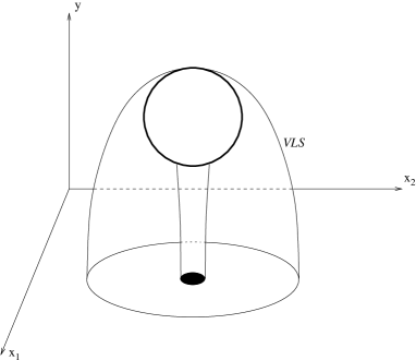
Figure 5: “Medusa” diagram: singularity, velocity of light surface and cylinder connecting the singularity ($\partial\hat{\Sigma}$) to the $y=0$ plane, for the lifted sphere.

Looking at the next to leading order expansion of the metric for $R^{2}+y^{2}\rightarrow\infty$ we can derive the mass of these excitations of $AdS^{5}\times S^{5}$

$$M=\frac{(\beta R_{0}^{2})^{2}}{32\pi^{2}l_{P}^{8}}(\frac{1}{\beta}-1)$$ (3.40)

which is clearly negative and, for fixed $R_{AdS}$, tends to minus infinity for $\beta\rightarrow 0^{-}$.

4 Singular solutions: generic properties

In this section we will prove the following

Theorem 4.1.

Geometries of the type studied in Section 2 have closed timelike curves if and only if $\partial\hat{\Sigma}\neq\emptyset$

In particular standard LLM geometries are free of CTCs as well as all geometries seeded by boundary conditions such that $\partial\hat{\Sigma}=\emptyset$ and

$$\frac{1}{2}-z_{0}(x_{1},x_{2})=\rho(x_{1},x_{2})\quad 0\leq\rho\leq 1$$ (4.1)

On the other hand, whenever $\rho>1$ or $\rho<0$, (and thus $\partial\hat{\Sigma}\neq\emptyset$), we have CTCs in the spacetime.

We will divide the proof into the 2 subsections 4.1 and 4.3. In subsection 4.2 we will comment on the generic (Lorentz) topology of the solutions and show that some of the interesting features of the examples in Sections 3.4 and 3.5 are indeed quite general.

4.1 Sufficient condition for CTCs

It’s easy to show that when $\partial\hat{\Sigma}\neq\emptyset$ we have CTCs.
Looking at the asymptotic expansion for large values of $x_{1}^{2}+x_{2}^{2}+y^{2}$ in Section 2.2, we can see that the vector field

$$\partial_{\psi}\equiv\frac{1}{\sqrt{V_{1}^{2}+V_{2}^{2}}}(V_{1}\partial_{1}+V_{2}\partial_{2})$$ (4.2)

has closed, almost circular orbits at infinity. We can shift $V$ by a constant amount such that $V=0$ at a point $P\in\partial\hat{\Sigma}$ with $\partial_{y}z(P)\neq 0$ and the orbits of $\partial_{\psi}$ are closed around $P$. Let’s assume for definiteness that $z(P)=-\frac{1}{2}$. In a neighborhood of P we have

$$z(x_{1},x_{2},y)\approx-\frac{1}{2}+\delta z$$ (4.3)

$$V_{i}(x_{1},x_{2},y)\approx\delta V_{i}$$ (4.4)

where $\delta z$ and $\delta V_{i}$ are linear in the co-ordinates $(x_{1}-x(P),x_{2}-x(P),y-y(P))$. The metric of the sections $\{x_{1},x_{2},y\}$ is (recalling that $h^{4}=\frac{1/4-z^{2}}{y^{2}}$),

$$\begin{split}\tilde{g}&=\begin{pmatrix}h^{2}-h^{-2}V_{1}^{2}&-h^{-2}V_{1}V_{2}&0\\ -h^{-2}V_{1}V_{2}&h^{2}-h^{-2}V_{2}^{2}&0\\ 0&0&h^{2}\end{pmatrix}\approx\\ &\approx\frac{1}{y(P)\sqrt{\delta z}}\begin{pmatrix}\delta z-y(P)^{2}\delta V_{1}^{2}&y(P)^{2}\delta V_{1}\delta V_{2}&0\\ y(P)^{2}\delta V_{1}\delta V_{2}&\delta z-y(P)^{2}\delta V_{2}^{2}&0\\ 0&0&\delta z\end{pmatrix}\end{split}$$ (4.5)

The vectors

$$\begin{split}&\partial_{\psi}\\ &\partial_{\sigma}\equiv\frac{1}{\sqrt{V_{1}^{2}+V_{2}^{2}}}(-V_{2}\partial_{1}+V_{1}\partial_{2})\\ &\partial_{y}\end{split}$$ (4.6)

are eigenvectors of $\tilde{g}$ with eigenvalues respectively

$$(h^{2}-h^{-2}(V_{1}^{2}+V_{2}^{2})\,,\,h^{2}\,,\,h^{2})\approx\frac{1}{y(P)\sqrt{\delta z}}(\delta z-y(P)^{2}\delta V^{2}\,,\,\delta z\,,\,\delta z)$$ (4.7)

Thus for

$$\delta z-y(P)^{2}\delta V^{2}<0$$ (4.8)

the sections are timelike. This equation also shows that the velocity of light surface always touches the singularity where $V=0$, as shown in Figure 6.

The opening of the lightcone is given by

$$\tan\theta=h^{-4}(V_{1}^{2}+V_{2}^{2})-1\approx\frac{y_{(}P)^{2}}{\delta z}\delta V^{2}-1$$ (4.9)

Thus any closed curve going around $P$ in the sense indicated by $\partial_{\psi}$ is a CTC provided that we stay close enough to $P$ and $\partial\hat{\Sigma}$ (on which we recall $\delta z=0$ by definition). Since the CTCs are not hidden by a horizon, also in this general case a CTC passes through any point of the spacetime.

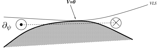
Figure 6: $\partial\hat{\Sigma}$ and the VLS touching at $V^{2}=0$.

4.2 (Lorentz) topology

In the case discussed in Section 3.5 we have $z_{0}=\frac{1}{2}$ on the entire $\{x_{1},x_{2}\}$ plane and $z=-\frac{1}{2}$ on a sphere centered on the $y$ axis. The appearance of contractible CTCs is excluded by a detailed analysis of the structure of the metric. The Lorentz topology is thus nontrivial, as one could expect in order to preserve the regularity of the local structure of spacetime. The same analysis shows that the topology of the $\{x_{1},x_{2},y\}$ sections is still $\mathbb{R}^{2}\times\mathbb{R}^{+}$, even if at first sight one would say that a sphere has been removed. This is essentially due to the non vanishing of $V_{\varphi}$ along the $y$ axis in the segment between the $y=0$ plane and the sphere.

Assume we have a connected subset of $\partial\hat{\Sigma}$ which is not attached to the $\{x_{1},x_{2}\}$ plane. We can analytically continue $z$ (and thus $\Phi$) to the $|z|>\frac{1}{2}$ side of $\partial\hat{\Sigma}$. We will necessarily encounter some pole singularity in the equation for $\Phi$, as $\delta$ sources centered on some point $Q$. In a neighborhood of such a point $(\vec{x}_{0},y_{0})$ we have to leading order

$$z\approx\sigma y_{0}^{2}\frac{1}{\sqrt{(y-y_{0})^{2}+R^{2}}}$$ (4.10)

$$V\approx V_{\varphi}\mathrm{d}\varphi\qquad V_{\varphi}\approx\sigma y_{0}\left(1-\frac{y-y_{0}}{\sqrt{(y-y_{0})^{2}+R^{2}}}\right)$$ (4.11)

where $R,\varphi$ are polar coordinates in $x_{1},x_{2}$ centered on $\vec{x}_{0}$. By continuity, we can argue that in a neighborhood of this $Q$, for $y<y_{0}$, the vector $V_{i}\partial_{i}$ is circulating around a line $\mathcal{L}$ on which it doesn’t vanish. Going locally to polar coordinates centered on the intersection of this line with a constant $y$ plane, we have that

$$g_{\varphi\varphi}=-h^{-2}V_{\phi}^{2}+R^{2}h^{2}$$ (4.12)

is non vanishing at $R=0$ and thus the line $\mathcal{L}$ is topologically a cylinder. As in section 3.5, the shape of the space-time around such a point $Q$ is similar to the “Medusa” diagram of Figure 5. We expect that several disconnected components of $\partial\hat{\Sigma}$ may give rise to more complicated geometrical structures.

4.3 Necessary condition for CTCs

In this Section we will show that if $\partial\hat{\Sigma}=\emptyset$, then there are no CTCs. Looking at the metric (2.1) it is clear that if the determinant $\tilde{g}$ of the spatial section $\{x_{1},x_{2},y\}$ is positive, then there cannot be CTCs. We recall from Section 2 that

$$z(x_{1},x_{2},y)=\frac{1}{2}-\frac{y^{2}}{\pi}\int\frac{\rho(x_{1}^{\prime},x_{2}^{\prime})\mathrm{d}^{2}x}{\left[(x_{1}-x_{1}^{\prime})^{2}+(x_{2}-x_{2}^{\prime})^{2}+y^{2}\right]^{2}}$$ (4.13)

$$V_{i}=-\frac{1}{\pi}\epsilon_{ij}\int\frac{(x_{j}-x_{j}^{\prime})\rho(x_{1}^{\prime},x_{2}^{\prime})\mathrm{d}^{2}x^{\prime}}{[(x_{1}-x_{1}^{\prime})^{2}+(x_{2}-x_{2}^{\prime})^{2}+y^{2}]^{2}}$$ (4.14)

and the determinant of the three dimensional sections

$$\tilde{g}=h^{4}-V^{2}=\frac{1/4-z^{2}}{y^{2}}-V^{2}=\\ =\frac{1}{\pi}\int\frac{\rho(x_{1}^{\prime},x_{2}^{\prime})\mathrm{d}^{2}x}{\left[(x_{1}-x_{1}^{\prime})^{2}+(x_{2}-x_{2}^{\prime})^{2}+y^{2}\right]^{2}}-\frac{y^{2}}{\pi^{2}}\left(\int\frac{\rho(x_{1}^{\prime},x_{2}^{\prime})\mathrm{d}^{2}x}{\left[(x_{1}-x_{1}^{\prime})^{2}+(x_{2}-x_{2}^{\prime})^{2}+y^{2}\right]^{2}}\right)^{2}+\\ -\sum_{i=1,2}\frac{1}{\pi^{2}}\left(\int\frac{(x_{i}-x_{i}^{\prime})\rho(x_{1}^{\prime},x_{2}^{\prime})\mathrm{d}^{2}x^{\prime}}{[(x_{1}-x_{1}^{\prime})^{2}+(x_{2}-x_{2}^{\prime})^{2}+y^{2}]^{2}}\right)^{2}$$ (4.16)

Any possible geometry seeded by a function $\rho(x_{1},x_{2})$ with $0\leq\rho\leq 1$ can be approximated as well as desired by a piecewise constant $\bar{\rho}$ such that $\bar{\rho}=0,1$. So it is enough to prove that the determinant is positive for standard LLM geometries defined by droplets of density $\rho=1$.

We will prove that, given any possible distribution of droplets $\mathcal{D}$ and any point $P\equiv(x_{1}(P),x_{2}(P),y)$, there is a halfplane $\Pi$ distribution for which $z(P)$ is the same as for the original distribution and $V(P)^{2}$ is larger. In this way the determinant $\tilde{g}(P)_{\Pi}$ for the halfplane distribution is smaller than the original determinant $\tilde{g}_{\mathcal{D}}$ . As noted already in [1] a halfplane distribution corresponds to the maximally supersymmetric plane wave and for this metric the determinant always satisfies the relation

$$\tilde{g}_{\Pi}=\frac{1/4-z^{2}}{y^{2}}-V_{\Pi}^{2}=0$$ (4.17)

So we have $\tilde{g}_{\mathcal{D}}\geq\tilde{g}_{\Pi}=0$.

We first make some assumptions in order to simplify the proof. Given the point $P\equiv(x_{1}(P),x_{2}(P),y)$ we move the origin of the $\{x_{1},x_{2}\}$ plane to $(x_{1}(P),x_{2}(P))$. We then define a 2-vector $\tilde{V}$ such that $\tilde{V}^{2}=V^{2}$

$$\tilde{V}_{i}[\mathcal{D}](P)=\frac{1}{\pi}\int_{\mathcal{D}}\frac{x_{i}}{\left(x_{1}^{2}+x_{2}^{2}+y^{2}\right)^{2}}\mathrm{d}^{2}x$$ (4.18)

$$\tilde{V}_{1}^{2}+\tilde{V}_{2}^{2}=V_{1}^{2}+V_{2}^{2}$$ (4.19)

where $\mathcal{D}$ is the union of all the droplets. We also have

$$z_{\mathcal{D}}(P)=\frac{1}{2}-\Delta_{\mathcal{D}}z=\frac{1}{2}-\frac{y^{2}}{\pi}\int_{\mathcal{D}}\frac{1}{\left(x_{1}^{2}+x_{2}^{2}+y^{2}\right)^{2}}\mathrm{d}^{2}x$$ (4.20)

We identify the direction of $\tilde{V}$ with the $x_{2}$ axis. Let us assume that the droplets are all contained in the strip

$$x_{\text{min}}\leq x_{2}\leq x_{\text{max}}$$ (4.21)

where one or even both of $x_{\text{min}}$ and $x_{\text{max}}$ can also be infinite. A distribution corresponding to the (half)plane $\Pi_{0}$ defined by $x_{2}\geq x_{\text{min}}$ will give us

$$z_{\Pi_{0}}(P)\leq z_{\mathcal{D}}(P)$$ (4.22)

since $\mathcal{D}\subseteq\Pi_{0}$

The equality holds just in the case that the original distribution is already a halfplane. In all the other cases, we take a halfplane $\Pi$ defined by

$$x_{2}\geq x$$ (4.23)

with $x>x_{\text{min}}$ such that

$$z_{\Pi}(P)=z_{\mathcal{D}}(P)$$ (4.24)

Figure 7: Changing $\mathcal{D}$ into $\Pi$

We note that for a generic domain $\mathcal{D}$ we have the following relation between $\Delta_{\mathcal{D}}z$ and $\tilde{V}_{2}[\mathcal{D}](P)$

$$\tilde{V}_{2}[\mathcal{D}](P)=\frac{\Delta_{\mathcal{D}}z}{y^{2}}\langle x_{2}\rangle_{\mathcal{D}}$$ (4.25)

with

$$\langle x_{2}\rangle_{\mathcal{D}}=\frac{1}{\pi}\int_{\mathcal{D}}\frac{x_{2}\mathrm{d}^{2}x}{\left(x_{1}^{2}+x_{2}^{2}+y^{2}\right)^{2}}\left(\frac{1}{\pi}\int_{\mathcal{D}}\frac{\mathrm{d}^{2}x}{\left(x_{1}^{2}+x_{2}^{2}+y^{2}\right)^{2}}\right)^{-1}=$$ (4.26)

$$=\int x_{2}\,\,\mu_{\mathcal{D}}(x_{2})\mathrm{d}x_{2}$$

$$\mu_{\mathcal{D}}(x_{2})=\frac{1}{\pi}\int_{\mathcal{D}}\frac{\mathrm{d}x_{1}}{\left(x_{1}^{2}+x_{2}^{2}+y^{2}\right)^{2}}\left(\frac{1}{\pi}\int_{\mathcal{D}}\frac{\mathrm{d}x_{1}\mathrm{d}x_{2}}{\left(x_{1}^{2}+x_{2}^{2}+y^{2}\right)^{2}}\right)^{-1}$$ (4.27)

$$\int\,\,\mu_{\mathcal{D}}(x_{2})\mathrm{d}x_{2}=1$$ (4.28)

Thus $\mu_{\mathcal{D}}(x_{2})$ acts as a normalized weight function.

From the definition of $\mu_{\mathcal{D}}(x_{2})$ and from the fact that, by definition of $\Pi$

$$\Delta_{\mathcal{D}}z=\Delta_{\Pi}z$$ (4.29)

i.e.

$$\frac{1}{\pi}\int_{\mathcal{D}}\frac{1}{\left(x_{1}^{2}+x_{2}^{2}+y^{2}\right)^{2}}\mathrm{d}^{2}x=\frac{1}{\pi}\int_{\Pi}\frac{1}{\left(x_{1}^{2}+x_{2}^{2}+y^{2}\right)^{2}}\mathrm{d}^{2}x$$ (4.30)

one can easily see that

$$\mu_{\Pi}(x_{2})\geq\mu_{\mathcal{D}}(x_{2})\quad,\quad x_{2}\geq x$$ (4.31)

$$\mu_{\Pi}(x_{2})=0\quad,\quad x_{2}<x$$ (4.32)

We have

$$\langle x_{2}\rangle_{\Pi}=x+\langle(x_{2}-x)\rangle_{\Pi}=\\ =x+\int\mu_{\Pi}(x_{2})(x_{2}-x)\mathrm{d}x_{2}\geq x+\int_{x_{2}>x}\mu_{\mathcal{D}}(x_{2})(x_{2}-x)\mathrm{d}x_{2}\,>\,\langle x_{2}\rangle_{\mathcal{D}}$$ (4.33)

The last inequality holds because

$$\langle x_{2}\rangle_{\mathcal{D}}=x+\int\mu_{\mathcal{D}}(x_{2})(x_{2}-x)\mathrm{d}x_{2}=\\ =x+\int_{x_{2}>x}\mu_{\mathcal{D}}(x_{2})(x_{2}-x)\mathrm{d}x_{2}+\int_{x_{2}<x}\mu_{\mathcal{D}}(x_{2})(x_{2}-x)\mathrm{d}x_{2}$$ (4.34)

and the last term is clearly negative.

Recalling (4.25) and (4.29) we conclude

$$\tilde{V}_{2}[\Pi](P)>\tilde{V}_{2}[\mathcal{D}](P)$$ (4.35)

and thus we have

$$\tilde{g}_{\mathcal{D}}=\frac{1/4-z_{\mathcal{D}}(P)^{2}}{y^{2}}-V_{\mathcal{D}}^{2}>\frac{1/4-z_{\Pi}(P)^{2}}{y^{2}}-V_{\Pi}^{2}=0$$ (4.36)

The case $y=0$

In the proof we have implicitly assumed $y>0$. In the limit $y\rightarrow 0$ one can argue, by continuity

$$\tilde{g}_{\mathcal{D}}\geq 0$$ (4.37)

With a bit of effort, we can prove that the equality holds only for the halfplane.

Instead of choosing $x$ in order to fix $z(P)$ we decide to fix

$$\lim_{y\rightarrow 0}\frac{1/4-z^{2}}{y^{2}}(P)$$ (4.38)

which is finite since by hypotheses $z\rightarrow\pm\frac{1}{2}$ and is even in $y$. Recalling that

$$\lim_{y\rightarrow 0}\frac{y^{2}}{\pi}\int_{\mathcal{D}}\frac{\mathrm{d}^{2}x}{\left(x_{1}^{2}+x_{2}^{2}+y^{2}\right)^{2}}=\begin{cases}1&P\in\mathcal{D}\\ 0&P\in\bar{\mathcal{D}}\end{cases}$$ (4.39)

we have

$$\frac{1/4-z^{2}}{y^{2}}\rightarrow\begin{cases}\frac{1}{y^{2}}\Delta_{\mathcal{D}}z\rightarrow\frac{1}{\pi}\int_{\mathcal{D}}\frac{\mathrm{d}^{2}x}{\left(x_{1}^{2}+x_{2}^{2}\right)^{2}}&P\in\bar{\mathcal{D}}\\ -\frac{1}{y^{2}}\Delta_{\bar{\mathcal{D}}}z\rightarrow-\frac{1}{\pi}\int_{\bar{\mathcal{D}}}\frac{\mathrm{d}^{2}x}{\left(x_{1}^{2}+x_{2}^{2}\right)^{2}}&P\in\mathcal{D}\end{cases}$$ (4.40)

Noting that $V_{\mathcal{D}}=-V_{\bar{\mathcal{D}}}$, in both cases we can use the same argument as for $y\neq 0$ provided that we change $\mathcal{D}$ into $\bar{\mathcal{D}}$ when $P\in{\mathcal{D}}$. Thus $\tilde{g}\geq 0$ and again the equality holds only for the halfplane.

5 Supergravity singularities and dual field theories

There already exist in the literature on $AdS/CFT$ duality, some indications that geometries with naked time machines are related to non-physical phenomenon in the dual gauge theory. The dual picture should provide a field theory interpretation for the quantum mechanism at work in the resolution of these pathologies, possibly through a careful treatment of unitarity.

In particular, the overrotating solutions of [30] are exactly of this type and as already noted in that paper, and further elucidated in [38, 39], the operator in the corresponding D-brane configuration that takes an underrotating geometry to an overrotating one is non-unitary.

In that case it was first noticed [38] that the overrotating geometries have a VLS that repulses all geodesics that approach from the outside, and thus the region of CTCs is effectively removed from the space-time. It was then noticed in a series of works on the enhancon mechanism that incorporating extra charge sources one can remove the causality violating region[40]. A similar idea is developed for example also in [41]. Our naked time machines do not have a repulsive VLS and as a consequence this method for removing the singularity cannot be applied here.

That some form of chronology protection mechanism should however be present has been conjectured in [31]. In this paper the rotationally symmetric singular configurations that we have studied in Section 3.4 are noted to not have a description in terms of the dual free fermion picture as they violate the Pauli exclusion principle.

In general relativity and in supergravity there are of course many geometries that contain CTCs and naked singularities. Is it possible that a similar principle could also rule out those geometries? In particular is it possible that these geometries are in general related to non-unitarity in the dual gauge theories? The violation of the Pauli exclusion principle suggests that our naked time machines may more generally be related to some non-unitary behaviour in the dual gauge theory.

The conformal dimension $\Delta$ of an operator in the $CFT$ dual to an asymptotically $AdS_{5}\times S^{5}$ geometry is equal to the mass or angular momentum ($M=J$ as a consequence of the BPS condition) of the configuration. For a solution seeded by a density distribution $\rho$

$$\Delta=M=\frac{1}{8\pi^{2}l_{P}^{8}}\left[\frac{1}{\pi}\int\rho\frac{1}{2}(x_{1}^{2}+x_{2}^{2})-\left(\frac{1}{\pi}\int\rho\frac{1}{2}\right)^{2}\right]$$ (5.1)

As noted in Section 3.4, for a density which is $\beta$ inside a disk, we have

$$M=\Delta=\frac{\beta R_{AdS}^{8}}{32\pi^{2}l_{P}^{8}}(\frac{1}{\beta}-1)$$ (5.2)

From the CFT point of view a configuration with $\beta\gtrsim 1$ can be seen as a “small” deformation of a configuration with $\beta=1$ and slightly larger radius. Equation (5.2) shows that this deformation corresponds to an operator with negative conformal dimension.

In general we expect, even though we cannot prove it directly, that configurations with $\rho$ not between 0 and 1 correspond to deformations of the $CFT$ by negative conformal dimension operators. As seen in Section 3.5, solutions with more general boundary conditions can still be interpreted as continuous deformations of solutions seeded by density distributions and a similar argument should also relate them to operators of negative conformal dimension.

In a series of papers [28] all unitary irreducible representations of the relevant superconformal algebra, $su(2,2|N)$, are found and in particular unitarity requires that they have positive conformal dimension. The “unphysical” geometries that we have studied in this paper then apparently correspond to deformations by non-unitary operators (with negative conformal dimension) in the dual $CFT$. This observation together with the observed violation of the Pauli exclusion principle provides strong evidence for the existence of a theorem, for $1/2$ BPS configurations in IIB supergravity, relating the chronology protection conjecture to unitarity in the dual $CFT$.

Appendix A Plane wave solutions

Given any supersymmetric solution in supergravity, and in particular in type IIB, one can construct a Killing vector $\kappa$ by forming bilinears of the Killing spinors $\psi$

$$\kappa^{M}=\bar{\psi}\Gamma^{M}\psi$$ (A.1)

In type IIB supergravity, we have $\kappa^{M}\kappa_{M}=0$ [37].

For the geometry studied in [1] and in this paper the timelike Killing vector $\partial_{t}$ is obtained by adding one of these bilinears to a Killing vector coming from the $SO(4)\times SO(4)$ symmetry. We will briefly show that such timelike Killing vector can be built only when the bilinear $\kappa$ is not covariantly constant (c.c.). Any plane wave geometry in type IIB has 16 Killing spinors whose bilinears are constant multiple of the c.c. Killing vector of the metric [43]. If a plane wave is to be in the class of solutions constructed in [1], it will have 16 extra Killing spinors and thus must be the maximally supersymmetric pane wave studied in [33].

We refer to Appendix A of [1] for notation and conventions.

A.1 Ansatz and basic assumptions

The supersymmetric type IIB solutions under examination are described by

$$\mathrm{d}s^{2}=g_{\mu\nu}\mathrm{d}x^{\mu}\mathrm{d}x^{\nu}+\mathrm{e}^{H+G}\mathrm{d}\Omega^{2}_{3}+\mathrm{e}^{H-G}\mathrm{d}\mathaccent 869{\Omega}_{3}^{2}$$ (A.2)

$$F_{(5)}=F_{\mu\nu}\mathrm{d}x^{\mu}\wedge\mathrm{d}x^{\nu}\wedge\mathrm{d}\Omega+\mathaccent 869{F}_{\mu\nu}\mathrm{d}x^{\mu}\wedge\mathrm{d}x^{\nu}\wedge\mathrm{d}\mathaccent 869{\Omega}$$ (A.3)

A supersymmetric supergravity solution with just the $F_{5}$ field strength turned on is characterized by a non vanishing 32 dimensional complex spinor $\eta$ satisfying

$$\nabla_{M}\eta+\frac{\mathrm{i}}{480}\Gamma_{M_{1}M_{2}M_{3}M_{4}M_{5}}F_{(5)}^{M_{1}M_{2}M_{3}M_{4}M_{5}}\Gamma_{M}\eta=0$$ (A.4)

Due to our symmetry assumptions, the generic solution can be written as

$$\eta=\varepsilon_{a,b}\otimes\chi_{a}\otimes\tilde{\chi}_{b}$$ (A.5)

with $\varepsilon_{a,b}$ an 8 dimensional spinor and $\chi_{a}$,$\chi_{b}$ 2 dimensional spinors obeying the Killing spinor equation on the Euclidean 3-sphere

$$\bar{\nabla}_{c}\chi=\alpha\frac{\mathrm{i}}{2}\sigma_{c}\chi$$ (A.6)

with $\alpha=a,b$ respectively, $\sigma_{c}$ in the Clifford algebra of $SO(3)$ and $\bar{\nabla}_{c}$ the standard covariant derivative on the Euclidean 3-sphere. Integrability conditions imply $\alpha=\pm 1$. There are $2$ linearly independent solutions for each value of $\alpha$ [44, 45].

A.2 Spinor bilinears

We define the set of spinor bilinears

$$\begin{split}&K_{\mu}=-\bar{\varepsilon}\gamma_{\mu}\varepsilon\qquad f_{1}=\mathrm{i}\bar{\varepsilon}\sigma_{1}\varepsilon\qquad f_{2}=\mathrm{i}\bar{\varepsilon}\sigma_{2}\varepsilon\\ &\bar{\varepsilon}=\varepsilon^{\dagger}\gamma_{0}\end{split}$$ (A.7)

One can show that

$$\nabla_{\mu}K_{\nu}=\mathrm{e}^{-\frac{3}{2}(H+G)}F_{\mu\nu}f_{2}+\mathrm{e}^{-\frac{3}{2}(H-G)}\tilde{F}_{\mu\nu}f_{1}$$ (A.8)

from which we can see that $K_{\mu}$ is a Killing vector for $g_{\mu\nu}$ and by Fierz rearrengment one can show that

$$K^{2}=-f_{1}^{2}-f_{2}^{2}$$ (A.9)

The standard ten dimensional Killing vector coming from the sandwich of the spinors is given by, in ten dimensional covariant tangent space components

$$\kappa=\left(K(\chi^{\dagger}\chi)(\tilde{\chi}^{\dagger}\tilde{\chi}),f_{2}\chi^{\dagger}\vec{\sigma}\chi(\tilde{\chi}^{\dagger}\tilde{\chi}),-f_{1}(\chi^{\dagger}\chi)\tilde{\chi}^{\dagger}\vec{\sigma}\tilde{\chi}\right)$$

As expected from general considerations

$$\kappa^{2}=K^{2}(\chi^{\dagger}\chi)^{2}(\tilde{\chi}^{\dagger}\tilde{\chi})^{2}+f_{2}^{2}\sum_{a}(\chi^{\dagger}\sigma_{a}\chi)(\chi^{\dagger}\sigma_{a}\chi)(\tilde{\chi}^{\dagger}\tilde{\chi})^{2}+f_{1}^{2}(\chi^{\dagger}\chi)^{2}\sum_{a}(\tilde{\chi}^{\dagger}\sigma_{a}\tilde{\chi})(\tilde{\chi}^{\dagger}\sigma_{a}\tilde{\chi})=\\ =\left(-f_{1}^{2}-f_{2}^{2}+f_{2}^{2}+f_{1}^{2}\right)(\chi^{\dagger}\chi)^{2}(\tilde{\chi}^{\dagger}\tilde{\chi})^{2}=0$$ (A.10)

where we have used (A.9) and the basic fact, true for every two dimensional spinor $\zeta$ that

$$\sum_{a}(\zeta^{\dagger}\sigma_{a}\zeta)(\zeta^{\dagger}\sigma_{a}\zeta)=(\zeta^{\dagger}\zeta)^{2}$$

We also have that

$$\partial_{\hat{a}}(\chi^{\dagger}\chi)=\partial_{\tilde{a}}(\tilde{\chi}^{\dagger}\tilde{\chi})=0$$ (A.11)

and the vectors

$$J\equiv(\mathbf{0},\mathrm{e}^{\frac{1}{2}(H+G)}\chi^{\dagger}\vec{\sigma}\chi,\vec{0})\quad,\quad\tilde{J}\equiv(\mathbf{0},\vec{0},\mathrm{e}^{\frac{1}{2}(H-G)}\tilde{\chi}^{\dagger}\vec{\sigma}\tilde{\chi})$$ (A.12)

are Killing vectors, corresponding to the $SO(4)\times SO(4)$ isometry of our ansatz.

A.3 Analysis of bilinears

Assume that we have $f_{1,2}\neq 0$. In this case the vector $\kappa$ is Killing but not covariantly constant (c.c.). In [1] it is shown that we have

$$f_{1,2}\propto\mathrm{e}^{\frac{1}{2}(H\mp G)}$$ (A.13)

and thus also the vector

$$\kappa+J(\tilde{\chi}^{\dagger}\tilde{\chi})+\tilde{J}(\chi^{\dagger}\chi)=(K,\vec{0},\vec{0})$$ (A.14)

obtained as the sum of $\kappa$ and a Killing vector of the $SO(4)\times SO(4)$ symmetry, is a Killing vector for the full metric.

This vector is identified with $\partial_{t}$, which is possible since

$$K^{2}=-f_{1}^{2}-f_{2}^{2}<0$$ (A.15)

The fact that $f_{1,2}\neq 0$ is thus crucial for all the construction of the 1/2 supersymmetric solutions in [1]. From (A.8) one can see that the 16 independent Killing spinors $\eta$ do not have c.c. vector bilinear. Any plane wave geometry in type IIB has 16 Killing spinors whose bilinears are constant multiple of the c.c. Killing vector of the metric. The vector bilinears coming from these Killing spinors would then be null and c.c., with

$$f_{1}=f_{2}=0$$ (A.16)

which leads to

$$\kappa=(K(\chi^{\dagger}\chi)(\tilde{\chi}^{\dagger}\tilde{\chi}),\vec{0},\vec{0})$$

and $K^{2}=0$. In this case, by a similar construction to that of LLM [46], one can obtain a set of plane waves with $SO(4)\times SO(4)$ isometry and non vanishing five-form.

If one of these plane wave solutions could be obtained with the techniques presented in [1] it should have 16 extra Killing spinors whose bilinears $f_{1,2}$ do not vanish. This means that the solution must have 32 Killing spinors and then clearly it is the maximally supersymmetric plane wave of [33].

References

- [1] H. Lin, O. Lunin, and J. Maldacena, “Bubbling AdS space and 1/2 BPS geometries,” hep-th/0409174.
- [2] J. T. Liu and D. Vaman, “Bubbling 1/2 BPS solutions of minimal six-dimensional supergravity,” hep-th/0412242.
- [3] J. T. Liu, D. Vaman, and W. Y. Wen, “Bubbling 1/4 BPS solutions in type IIB and supergravity reductions on S**n x S**n,” hep-th/0412043.
- [4] D. Martelli and J. F. Morales, “Bubbling AdS(3),” JHEP 02 (2005) 048, hep-th/0412136.
- [5] Z. W. Chong, H. Lu, and C. N. Pope, “BPS geometries and AdS bubbles,” Phys. Lett. B614 (2005) 96–103, hep-th/0412221.
- [6] A. Ghodsi, A. E. Mosaffa, O. Saremi, and M. M. Sheikh-Jabbari, “LLL vs. LLM: Half BPS sector of N = 4 SYM equals to quantum Hall system,” hep-th/0505129.
- [7] H. Ebrahim and A. E. Mosaffa, “Semiclassical string solutions on 1/2 BPS geometries,” JHEP 01 (2005) 050, hep-th/0501072.
- [8] M. M. Sheikh-Jabbari and M. Torabian, “Classification of all 1/2 BPS solutions of the tiny graviton matrix theory,” JHEP 04 (2005) 001, hep-th/0501001.
- [9] S. Mukhi and M. Smedback, “Bubbling orientifolds,” hep-th/0506059.
- [10] M. Spalinski, “Some half-BPS solutions of M-theory,” hep-th/0506247.
- [11] I. Bena and N. P. Warner, “Bubbling supertubes and foaming black holes,” hep-th/0505166.
- [12] G. Mandal, “Fermions from half-BPS supergravity,” hep-th/0502104.
- [13] L. Grant, L. Maoz, J. Marsano, K. Papadodimas, and V. S. Rychkov, “Minisuperspace quantization of ’bubbling AdS’ and free fermion droplets,” hep-th/0505079.
- [14] V. Balasubramanian, D. Berenstein, B. Feng, and M.-x. Huang, “D-branes in Yang-Mills theory and emergent gauge symmetry,” JHEP 03 (2005) 006, hep-th/0411205.
- [15] D. Berenstein, “A toy model for the AdS/CFT correspondence,” JHEP 07 (2004) 018, hep-th/0403110.
- [16] S. Corley, A. Jevicki, and S. Ramgoolam, “Exact correlators of giant gravitons from dual N = 4 SYM theory,” Adv. Theor. Math. Phys. 5 (2002) 809–839, hep-th/0111222.
- [17] R. C. Myers and O. Tafjord, “Superstars and giant gravitons,” JHEP 11 (2001) 009, hep-th/0109127.
- [18] A. Buchel, “Coarse-graining 1/2 BPS geometries of type IIB supergravity,” hep-th/0409271.
- [19] P. Horava and P. G. Shepard, “Topology changing transitions in bubbling geometries,” JHEP 02 (2005) 063, hep-th/0502127.
- [20] S. S. Gubser and J. J. Heckman, “Thermodynamics of R-charged black holes in AdS(5) from effective strings,” JHEP 11 (2004) 052, hep-th/0411001.
- [21] D. Bak, S. Siwach, and H.-U. Yee, “1/2 BPS geometries of M2 giant gravitons,” hep-th/0504098.
- [22] J. McGreevy, L. Susskind, and N. Toumbas, “Invasion of the giant gravitons from anti-de Sitter space,” JHEP 06 (2000) 008, hep-th/0003075.
- [23] A. Hashimoto, S. Hirano, and N. Itzhaki, “Large branes in AdS and their field theory dual,” JHEP 08 (2000) 051, hep-th/0008016.
- [24] V. Balasubramanian, V. Jejjala, and J. Simon, “The library of Babel,” hep-th/0505123.
- [25] S. S. Gubser, “Curvature singularities: The good, the bad, and the naked,” Adv. Theor. Math. Phys. 4 (2002) 679–745, hep-th/0002160.
- [26] R. C. Myers, “Stress tensors and Casimir energies in the AdS/CFT correspondence,” Phys. Rev. D60 (1999) 046002, hep-th/9903203.
- [27] G. T. Horowitz and R. C. Myers, “The value of singularities,” Gen. Rel. Grav. 27 (1995) 915–919, gr-qc/9503062.
- [28] V.K. Dobrev and V.B. Petkova, “On the group theoretical approach to extended conformal supersymmetry: classification of multiplets”, Lett. Math. Phys. 9(1985), 287; V.K. Dobrev and V.B. Petkova, “All positive energy Unitary Irreducible Representations of extended conformal supersymmetry”, Phys. Lett.B162, (1985), 127.
- [29] S. W. Hawking, “The Chronology protection conjecture,” Phys. Rev. D46 (1992) 603–611.
- [30] J. C. Breckenridge, R. C. Myers, A. W. Peet, and C. Vafa, “D-branes and spinning black holes,” Phys. Lett. B391 (1997) 93–98, hep-th/9602065.
- [31] M. M. Caldarelli, D. Klemm, and P. J. Silva, “Chronology protection in anti-de Sitter,” hep-th/0411203.
- [32] M. Boni and P. J. Silva, “Revisiting the D1/D5 system or bubbling in AdS(3),” hep-th/0506085.
- [33] M. Blau, J. Figueroa-O’Farrill, C. Hull, and G. Papadopoulos, “A new maximally supersymmetric background of IIB superstring theory,” JHEP 01 (2002) 047, hep-th/0110242.
- [34] M. Blau, M. Borunda, M. O’Loughlin, and G. Papadopoulos, “The universality of Penrose limits near space-time singularities,” JHEP 07 (2004) 068, hep-th/0403252.
- [35] D. Berenstein, J. M. Maldacena, and H. Nastase, “Strings in flat space and pp waves from N = 4 super Yang Mills,” JHEP 04 (2002) 013, hep-th/0202021.
- [36] Y. Takayama and K. Yoshida, “Bubbling 1/2 BPS geometries and Penrose limits,” hep-th/0503057.
- [37] E. J. Hackett-Jones and D. J. Smith, “Type IIB Killing spinors and calibrations,” JHEP 11 (2004) 029, hep-th/0405098.
- [38] G. W. Gibbons and C. A. R. Herdeiro, “Supersymmetric rotating black holes and causality violation,” Class. Quant. Grav. 16 (1999) 3619–3652, hep-th/9906098.
- [39] C. A. R. Herdeiro, “Special properties of five dimensional BPS rotating black holes,” Nucl. Phys. B582 (2000) 363–392, hep-th/0003063.
- [40] L. Jarv and C. V. Johnson, “Rotating black holes, closed time-like curves, thermodynamics, and the enhancon mechanism,” Phys. Rev. D67 (2003) 066003, hep-th/0211097.
- [41] N. Drukker, “Supertube domain-walls and elimination of closed time-like curves in string theory,” Phys. Rev. D70 (2004) 084031, hep-th/0404239.
- [42] L. Cornalba and M. S. Costa, “Unitarity in the presence of closed timelike curves,” hep-th/0506104.
- [43] M. Blau, J. Figueroa-O’Farrill, and G. Papadopoulos, “Penrose limits, supergravity and brane dynamics,” Class. Quant. Grav. 19 (2002) 4753, hep-th/0202111.
- [44] M. Blau, “Killing spinors and SYM on curved spaces,” JHEP 11 (2000) 023, hep-th/0005098.
- [45] C. Bär, “Real Killing spinors and holonomy,” Communications in Mathematical Physics 154 (1993) 509–521.
- [46] G. Milanesi and M. O’Loughlin , unpublished, 2004.