Infrared Divergences in dS/CFT

Abstract:

dS/CFT gives a perturbatively gauge invariant definition of particle masses in de Sitter (dS) space. We show, in a toy model in which the graviton is replaced with a minimally coupled massless scalar field, that loop corrections to these masses are infrared (IR) divergent. We argue that this implies anomalous dependence of masses on the cosmological constant, in a true theory of quantum gravity. This is in accord with the hypothesis of Cosmological SUSY Breaking (CSB).

1 Introduction

The hypothesis of Cosmological Supersymmetry Breaking (CSB) is based on the idea [1] [2] [3] that quantum theories of stable, asymptotically de Sitter (AsdS) space-times exist and have a finite number of physical states. The (positive) cosmological constant, $\Lambda$,is an input parameter, which controls the number of states. The limit of vanishing $\Lambda$ is a super-Poincare invariant theory, but SUSY is broken for finite $\Lambda$: the operator which converges to the Poincare Hamiltonian $P_{0}$, does not commute with the SUSY charges.

Classical SUGRA supports such a picture, but suggests a relation between the gravitino mass and the c.c.: $m_{3/2}\sim\Lambda^{1/2}/M_{P}$. CSB is the proposal that the exponent $1/2$ in this relation is replaced by $1/4$ in the quantum theory. Given the interpretation of $\Lambda$ as a parameter controlling the number of states, this is a critical exponent, and it is plausible that it has fluctuation corrections. Indeed, low energy effective field theory cannot calculate the real relation between the gravitino mass and the c.c., since the c.c. is a relevant parameter and one must introduce a counterterm for it. The exponent above is just the “natural” relation of classical SUGRA, without fine tuning of the constant in the superpotential. If we accept such fine tuning, we can get any relation we want between $m_{3/2}$ and $\Lambda$ in effective field theory.

However, the necessity of canceling an infinite c.c. appears to be a short distance problem in effective field theory, and as such, does not seem to depend on the value of the c.c. . As a consequence, there has been considerable skepticism about CSB.

In [4], one of the authors presented an argument for the exponent $1/4$, based on crude approximations to the dynamics of the cosmological horizon in the static observer gauge for dS space. It was clear that from the static observer’s point of view, the enhanced exponent is an IR effect. However, since the argument relied on conjectures about the horizon dynamics, it has not convinced anyone. Skeptical observers want to understand where effective field theory reasoning breaks down. The work of [5] provided an important clue. In the static gauge most of the states in a quantum theory of dS space live on the horizon of the static observer. Local field theory can describe only a negligible fraction of the entropy. On the contrary, it was argued in [5] that in global coordinates, the entire Hilbert space may be well described by field theory. The contradiction between a finite number of states and the field theoretic description can be viewed as an IR cutoff, which restricts the global time coordinate to an interval of order $|t|\leq{\frac{R}{6}}\mathrm{ln}\left(RM_{P}\right)$ around the time symmetric point. The field theory also has a UV cutoff at a scale $M_{c}\sim\left({\frac{M_{P}}{R}}\right)^{1/2}$. This description is inappropriate for states containing black holes whose size scales like $R$, but there is a basis of field theoretic states in global coordinates, which may span the Hilbert space.

A simple way to restate this conclusion is to invoke the fact that the global description of dS space in field theory does not seem to break down until we contemplate introducing black holes on early time initial data slices, whose entropy exceeds that of the space-time. The combined UV and IR cutoffs prevent us from introducing such objects, and describes a cutoff field theory with a finite number of states. The field theory description of many of these states breaks down near the time-symmetric point, but near the upper and lower limits of $t$, it is a good approximation to their properties.

We have thus set up a framework in which IR divergences in a field theoretic treatment of dS space can be thought of as introducing non-classical dependence on the c.c. . It has often been argued that perturbative quantum gravity expanded around dS space is fraught with IR divergences. These claims have been less than convincing, because no-one had identified gauge invariant observables with which to check the physical meaning of the logarithmically growing graviton propagator. This problem is solved by dS/CFT [6][7][8]. In particular, the mass of a field in dS space is given a gauge invariant meaning: it is related to the dimension of a conformal field on the boundary.

The plan of this paper is as follows: in the next section we review dS/CFT, in the Wheeler-DeWitt formalism proposed by Maldacena. This allows perturbative calculations to be performed in a straightforward manner, apparently troubled only by conventional UV divergences. In section 3 we perform one loop calculations of boundary dimensions in a variety of non-gravitational field theories. We find that when the theory contains a massless, minimally coupled scalar field with soft couplings, the dimensions are infected with IR logarithms. In the conclusions, we discuss the difficulties attendant on an extension of these calculations to perturbative quantum gravity.

2 Review of dS/CFT

In his talk at Strings 2001 in Mumbai [6], Witten proposed a sort of scattering theory for de Sitter space. The fundamental object was the path integral with fixed boundary conditions on $\mathcal{I}_{\pm}$. It was implicitly assumed that, as in asymptotically flat and Anti-deSitter spaces, a field theoretic approximation became exact near the boundaries of space-time. This assumption is open to criticism. It is likely that generic boundary conditions on fields on $\mathcal{I}_{-}$ will lead to Big Crunch space-times, rather than space-times which are future asymptotically dS. However, this criticism does not apply to perturbation theory, where the boundary conditions are infinitesimal perturbations of those corresponding to the dS vacuum. Witten’s prescription provides a perturbative definition of amplitudes in dS quantum gravity, which are invariant under diffeomorphisms that approach the identity near $\mathcal{I}_{\pm}$.

Somewhat later, Strominger proposed [7] that suitably defined boundary amplitudes should be the correlation functions of a Euclidean conformal field theory (CFT). An apparent difference with Witten’s proposal is the role of conformally covariant, rather than invariant amplitudes in dS/CFT. However, Maldacena [9] has emphasized that the operator dimensions, OPE coefficients and the like, of dS/CFT, are gauge invariant observables in the sense of Witten.

The boundary correlation functions defined by Strominger should certainly be conformally invariant, but it is not clear that they should obey the axioms of field theory. Analogous arguments would lead us to believe that the holographic dual of linear dilaton backgrounds [10] was a Lorentz invariant field theory. The calculations of Peet and Polchinski [11] show that it is not. In the dS/CFT case, the form of the two point function follows from conformal invariance alone, and does not give us enough of a clue to the nature of the holographic dual. As believers in the proposition that quantum dS space has only a finite number of states, the present authors are inclined to disbelieve that a CFT will be the exact description of the quantum theory.

For our present purposes, all of these issues of principle are somewhat beside the point. We want a definition of correlation functions on $\mathcal{I}_{\pm}$ which is perturbatively well defined and gauge invariant. Furthermore, we will be interested only in two point functions, and will not have to address the question of whether higher order correlators obey the axioms of CFT. We have found that the dS/CFT prescription advocated by Maldacena [8] is the most appropriate for our purposes. Maldacena observes that the Euclidean path integral on a space with the topology of a hemisphere defines a “wave function of the universe” which is a functional of fields on the boundary of the hemisphere. In leading semiclassical approximation, the geometry is the section of the round sphere metric

$${ds^{2}=d\theta^{2}+sin^{2}(\theta)d\Omega^{2}}$$

with $0\leq\theta\leq\theta_{0}$. Maldacena defines boundary correlators as the expansion coefficients of the logarithm of the wave function of the universe for fixed $\theta_{0}$. The analytic extrapolation $\theta_{0}\rightarrow{\frac{\pi}{2}}+it$, $t\rightarrow\infty$ defines correlation functions on $\mathcal{I}_{+}$. If the limiting correlation functions exist, they should be covariant under the conformal group of the sphere. In particular, if we work in planar coordinates on the upper triangle of the dS Penrose diagram

$$ds^{2}=\frac{1}{\eta^{2}}\left(-d\eta^{2}+d\mathbf{x}^{2}\right)$$

($\mathcal{I}_{+}$is at $\eta=0$) then the boundary two point function should have the form $|\mathbf{x}|^{-\Delta}$. For a free scalar field of mass $m^{2}$ this is indeed true, and the relation between mass and dimension is given by

$$\Delta_{\pm}=a=\frac{1}{2}\left(d-1\pm\sqrt{(d-1)^{2}-4m^{2}R^{2}}\right)$$

This is an analytic continuation (in the c.c.) of analogous formulas in AdS/CFT. Indeed, Maldacena’s proposal for the correlation functions is the direct analog of the calculation of Euclidean correlation functions in AdS/CFT.

The purpose of the present paper is to compute one loop corrections to $\Delta_{\pm}$ in simple field theory models. We will see that when the theory has a massless, minimally coupled scalar with soft couplings, these corrections are IR divergent.

3 Review of QFT in dS space

In this section we will introduce the principal formulae of QFT ind-dimensional de Sitter (dS^d) space, and fix our notation .

For a more complete discussion we refer to the excellent review paper [12].

3.1 Coordinate Systems

d-dimensional de Sitter dS^d can be realized as the manifold, embedded in $d+1$ dimensional Minkowski $\mathcal{M}^{d,1}$ space, defined by the equation

$$-X_{0}^{2}+X_{1}^{2}+\cdots X_{d}^{2}=R^{2}$$ (1)

where $R$ is the de Sitter radius.

The de Sitter metric is the standard metric induced by immersion in $\mathcal{M}^{d,1}$ with the usual flat metric. The isometry group of dS^d is $O(d,1)$ in fact this leave invariant both the hyperboloid defined by the equation (1) and the flat metric of $\mathcal{M}^{d,1}$.

For the most part, we will use planar coordinates

$$X^{0} = \sinh t-\frac{1}{2}x_{i}x_{i}e^{-t}$$

$$X^{i} = x^{i}e^{-t}$$ (2)

$$X^{d} = \cosh t-\frac{1}{2}x_{i}x_{i}e^{-t}$$

with $i=1,\ldots,d$ the metric take the form

$$ds^{2}=-dt^{2}+e^{-2t}dx_{i}dx_{i}$$

In these coordinates the spatial sections have flat Euclidean metric.

It is useful to introduce conformal coordinates too, defined by the transformation

$$\eta=e^{t}$$

The metric is conformally flat and takes the form

$$ds^{2}=\frac{1}{\eta^{2}}\left(-d\eta^{2}+dx_{i}dx_{i}\right)$$

with $i=1,\ldots,d$. In the following, unless otherwise stated, we will consider the Euclidean section of dS^d defined by the analytical continuation

$$\eta\rightarrow ix_{0}$$ (3)

after the transformation (3) the metric become

$$ds^{2}=-\frac{1}{x_{0}^{2}}\left(dx_{0}^{2}+dx_{i}dx_{i}\right)$$ (4)

in these coordinates the boundary of dS^d $\Sigma$ is given by the submanifold $x_{0}=\epsilon$ where $\epsilon\rightarrow 0$.

3.2 Geodesic Distance

The geodesic distance between two points $x$ and $x^{\prime}$ is

$$\mu(x,x^{\prime})=\int_{0}^{1}\left[g_{ab}\dot{x}^{a}(\lambda)\dot{x}^{b}(\lambda)\right]^{\frac{1}{2}}d\lambda,~{}~{}x^{a}(0)=x,~{}~{}x^{a}(1)=x^{\prime}$$

In the following we will often use the new variable

$$z=\cos^{2}\left(\frac{\mu}{2R}\right)$$

It is possible to show that

$$\cos\left(\frac{\mu(x,x^{\prime})}{R}\right)=\frac{\eta_{ab}X^{a}(x)X^{b}(x^{\prime})}{R^{2}}$$

with $X^{a}(x),~{}X^{b}(x^{\prime})\in\mathcal{M}^{d,1}$ embedding coordinates and $\eta_{ab}=$diag$(-1,1,\ldots,1)$.

Consequently we have

$$z = \cos^{2}\left(\frac{\mu}{2R}\right)$$

$$= \frac{1}{2}\left(1+\cos(\frac{\mu}{R})\right)$$

$$= \frac{1}{2}\left(1+\frac{\eta_{ab}X^{a}(x)X^{b}(x^{\prime})}{R^{2}}\right)$$

In the Euclidean conformally flat coordinates (4) we have

$$z=-\frac{(x_{0}-y_{0})^{2}+\left(\bar{x}-\bar{y}\right)^{2}}{x_{0}y_{0}}=-2+\frac{x_{0}^{2}+y_{0}{}^{2}+(\bar{x}-\bar{y})^{2}}{x_{0}y_{0}}$$

3.3 The Cut-off Prescription

Maldacena’s prescription defines the boundary correlators by analytic continuation in global time. We have proposed that these formulae should be cut off at a fixed global time $T$. IR divergences will appear as divergent behavior at large $T$. It is most convenient to do calculations in conformal coordinates. Thus we have to understand the effect of a global time cut-off in conformal coordinates.

The relation between the two coordinate systems is most simply understood by writing the embedding coordinates in terms of conformal coordinates. The slices of fixed embedding time and global time coincide:

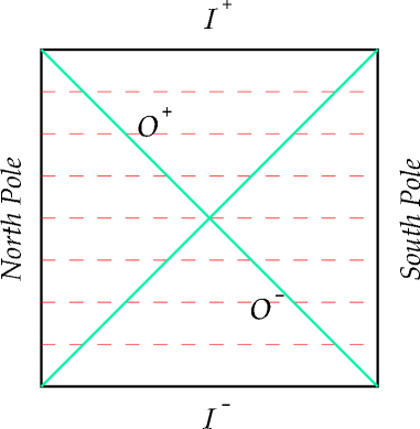
Figure 1: Global coordinates. Foliation of dS with compact spatial sections (spheres).

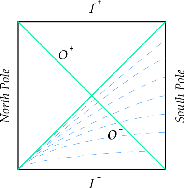
Figure 2: Flat coordinates. Foliation of dS with flat spatial sections.

$$X^{0}=\frac{R}{2}\left(\frac{x^{0}}{R}-\frac{R}{x^{0}}\right)-\frac{\mathbf{x}^{2}}{2x^{0}}$$

At $X^{0}=T$, see Fig. 2 and Fig. 2. This relation implies a maximal value of $|\mathbf{x}|$ for fixed $x^{0}$, as well as a maximal value of $x^{0}$ (which runs between $-\infty$ and $0$ in the conformal coordinate patch). The relation is

$$x_{\max}^{2}=-2x^{0}\left(T-x^{0}+\frac{R^{2}}{x^{0}}\right)$$

The maximal value of $x^{0}$ is the point at which $x_{max}=0$.

$$x_{max}^{0}\approx-{\frac{R^{2}}{T}}\ \ \ T\gg R$$

The maximal geodesic distance between two points on a give $x^{0}$ slice is ${\frac{x_{max}}{x_{max}^{0}}}$. The slice on which this distance is maximal is given by $x^{0}_{*}=-{\frac{2R^{2}}{T}}$. The geodesic distance on this slice is $o(T)$, while the maximum coordinate distance is $o(R)$. IR divergences will come predominantly from slices near this maximal slice.

Dirichlet boundary conditions on the $X^{0}=T$ surface become spatial Dirichlet boundary conditions on the spatial slices of conformal coordinates. On most of the slice of maximal geodesic size, the Dirichlet propagator will coincide with the usual Euclidean propagator defined by analytic continuation from the entire sphere. Thus, the boundary conditions will not affect the IR divergences.

3.4 Wave Function of the Universe

We are looking for a gauge invariant definition of the IR renormalization of the particle mass. The Wave Function of the Universe (WFU) will provide us with such a definition.

The WFU $\Psi[h_{ij},\phi_{0}]$ was first introduced by Hartle and Hawking in [13]. If $I[g,\phi]$ is the Euclidean action for gravity and a set of fields indicated by $\phi$, the Euclidean WFU is defined as the path integral

$$\Psi[h_{ij},\phi_{0}]=\int_{C}[dg][d\phi]e^{-I[g,\phi]}~{}$$ (5)

over a class $C$ of space-times with a compact space-like boundary $\Sigma$ on which the induced metric is $h_{ij}$ and over the field configurations $\phi$ with boundary value $\phi_{0}$. The boundary $\Sigma$ has only one connected component.

In the case $\Lambda>0$ we imagine a semiclassical expansion of the integral over Riemannian spaces with the topology of a hemisphere, expanded around the metric on the portion of the round sphere below polar angle $\theta_{0}$. We then analytically continue to the future half of Lorentzian dS space. This prescription corresponds to the choice of Euclidean vacuum in de Sitter space.

Given the WFU we can define the ”boundary two-point function” in the limit where the boundary is taken to $\mathcal{I^{+}}$

$$\frac{\delta\Psi[h_{ij},\phi_{0}]}{\delta\phi_{0}(\bar{x})\delta\phi_{0}(\bar{y})}$$

Once we expand around dS^d we find

$$\frac{\delta\Psi[h_{ij},\phi_{0}]}{\delta\phi_{0}(\bar{x})\delta\phi_{0}(\bar{y})}=C_{+}\frac{1}{(\bar{x}-\bar{y})^{2\Delta_{+}}}+C_{-}\frac{1}{(\bar{x}-\bar{y})^{2\Delta_{-}}}$$ (6)

, where $C_{\pm}$ are constants This form is dictated by conformal invariance. If $\lambda$ and $m$ are the coupling and the mass of the field $\phi$, in the classical Lagrangian, then $\Delta$ will be a function of $\lambda$ and $m$ and will provide a gauge invariant definition of the renormalized mass.

The Eq. (6) is the analogue of the boundary correlators defined in the AdS/CFT correspondence

$$Z[\phi_{0}]=\left\langle e^{\int d^{4}x\phi_{0}(x)O(x)}\right\rangle_{CFT}~{}\ ,~{}\phi(x_{0}=\epsilon)\sim\phi_{0}$$

$$\langle 0|O(\bar{x})O(\bar{y})|0\rangle=\frac{\delta Z}{\delta\phi_{0}(\bar{x})\delta\phi_{0}(\bar{y})}=\tilde{C}\frac{1}{(\bar{x}-\bar{y})^{2\tilde{\Delta}}}$$

There are however, important differences between the two cases. They stem from the fact that the Euclidean section of dS space is a spherical cap and has a conventional Dirichlet problem, different from the singular Dirichlet boundary conditions on the boundary of Euclidean AdS space. There are no large volume divergences in the Euclidean calculation. They appear only after extrapolation to infinite Lorentzian time. As a consequence, the divergent behavior comes as a combination of both powers $\Delta_{\pm}$. For fields corresponding to the principal series of dS representation theory, the real parts of $\Delta_{\pm}$ are equal.

The prescription to extract boundary two-point function in dS^d given by (6) was first pointed out by Maldacena in [8] and it is, as explained in this paper, different from the prescription used by Strominger and collaborators in [7], [14].

3.5 Representations of the dS^d Group

The scalar representation of the de Sitter group $SO(1,d)$ are classified according to the mass $m$ in the following series, see [15], [16]: the principal series

$$m^{2}\geqslant\left(\frac{d-1}{2R_{dS}}\right)$$

the complementary series

$$0<m^{2}<\left(\frac{d-1}{2R_{dS}}\right)$$

and the discrete series, whose only case of physical interest is $m^{2}=0$.

Under a Wigner-Inönü contraction to the Poincare group, only the representations of the principal series contract to representation of the Poincare Group.

Lowe and Güijosa [17] and Lowe [18] use the principal series to construct the dS/CFT correspondence. They stress the fact that when one replaces the dS isometry group with a q-deformed version, the unitary principal representation deform to a finite dimensional unitary representation of the quantum group.

The massive scalar particles in our formulae will always correspond to the principle series representations, so that the boundary dimensions all have the same real part. We will also use a massless, minimally coupled scalar, which is our toy model of the graviton.

4 Scalar Green Functions

In the next few subsections we will derive the scalar Green Functions relevant for our computations and their asymptotic behavior. As explained in the section on the cut-off procedure, we will not impose Dirichlet boundary conditions on the bulk propagators. The IR divergences, which are our principal concern, are not affected by the boundary conditions on the bulk propagator. For a more detailed discussion of dS Green functions, see for example [19], [20].

4.1 Maximally Symmetric Bitensors

The relevant geometric objects in maximally symmetric spaces, like dS, are the geodesic distance $\mu(x,x^{\prime})$ between two points $x$ and $x^{\prime}$, the unit tangent vectors $n_{\sigma}(x,x^{\prime})$ and $n_{\sigma^{\prime}}(x,x^{\prime})$ to the geodesic at $x$ and at $x^{\prime}$, the vector parallel propagator $g^{\mu}{}_{\nu^{\prime}}(x,x^{\prime})$ and the spinor parallel propagator $\Lambda^{\alpha}{}_{\beta^{\prime}}(x,x^{\prime})$.

The geodesic distance is by definition the distance along the geodesic $x^{a}(\lambda)$ connecting $x$ and $x^{\prime}$

$$\mu(x,x^{\prime})=\int_{0}^{1}\left[g_{ab}\dot{x}^{a}(\lambda)\dot{x}^{b}(\lambda)\right]^{\frac{1}{2}}d\lambda,~{}~{}x^{a}(0)=x,~{}~{}x^{a}(1)=x^{\prime}$$

The vectors $n_{\sigma},n_{\sigma^{\prime}}$ are defined by

$$n_{\sigma}=\nabla_{\sigma}\mu(x,x^{\prime})\qquad\mathrm{and}\qquad n_{\sigma^{\prime}}=\nabla_{\sigma^{\prime}}\mu(x,x^{\prime})\$$

where $\nabla_{\sigma}$ is the covariant derivative. We note that

$$n_{\sigma}=-g_{\sigma}{}^{\rho^{\prime}}n_{\rho^{\prime}}\$$

The vector and spinor parallel propagators are defined by

$$V^{\mu}(x) = g^{\mu}{}_{\nu^{\prime}}(x,x^{\prime})V^{\nu^{\prime}}(x^{\prime})\$$ (7)

$$\psi^{\alpha}(x) = \Lambda^{\alpha}{}_{\beta^{\prime}}(x,x^{\prime})\psi^{\beta^{\prime}}(x^{\prime})$$ (8)

for every parallel-transported vector $V^{\mu}(x)$ and spinor $\psi^{\alpha}(x)$, respectively.

Tensors that depend on two points $x$ and $x^{\prime}$ on the manifold are called bitensor. We will say that a bitensor is maximally symmetric if is invariant under any isometry of the manifold. It can be proved that any maximally symmetric bitensor can be expressed as a sum of products of $g^{\mu}{}_{\nu^{\prime}},~{}g_{\mu\nu},~{}g_{\mu^{\prime}\nu^{\prime}}{},~{}\mu,~{}n_{\sigma}$ and $n_{\sigma^{\prime}}$. Furthermore the coefficients of these terms are functions only of the geodesic distance $\mu(x,x^{\prime})$.

The covariant derivatives of the above bitensors are given by

$$\nabla_{\mu}n_{\nu} = A\,(g_{\mu\nu}-n_{\mu}n_{\nu})\$$

$$\nabla_{\mu^{\prime}}n_{\nu} = C\,(g_{\mu^{\prime}\nu}+n_{\mu^{\prime}}n_{\nu})\$$

$$\nabla_{\mu}g_{\nu\rho^{\prime}} = -(A+C)\,(g_{\mu\nu}n_{\rho^{\prime}}+g_{\mu\rho^{\prime}}n_{\nu})\$$ (9)

$$\nabla_{\mu}\Lambda^{\alpha}{}_{\beta^{\prime}} = \frac{1}{2}(A+C)\,[\,(\Gamma_{\mu}\Gamma^{\nu}n_{\nu}-n_{\mu})\,\Lambda]^{\,\alpha}{}_{\beta^{\prime}}\$$

$$\nabla_{\mu^{\prime}}\Lambda^{\alpha}{}_{\beta^{\prime}} = -\frac{1}{2}(A+C)\,[\,(\Gamma_{\mu^{\prime}}\Gamma^{\nu^{\prime}}n_{\nu^{\prime}}-n_{\mu^{\prime}})\,\Lambda]^{\,\alpha}{}_{\beta^{\prime}}\$$

where $A$ and $C$ are the following functions of the geodesic distance:

$$\mathrm{for\,\,\,\,\mathbf{R}^{d}:}\qquad A(\mu)=\frac{1}{\mu}\,\qquad C(\mu)=-\frac{1}{\mu}\,$$

$$\mathrm{for\,\,\,\,dS~{}and~{}AdS:}\qquad A(\mu)=\frac{1}{R}\cot\frac{\mu}{R}\,\qquad C(\mu)=-\frac{1}{R\sin\left(\frac{\mu}{R}\right)}\$$ (10)

The radius $R$ is real for dS^d and it is $R=i\tilde{R}$ with $\tilde{R}$ real for AdS^d. The covariant gamma matrices satisfy the usual relation $\{\Gamma^{\mu},\Gamma^{\nu}\}=2g^{\mu\nu}$.

4.2 Bulk Two-Point Function

In this subsection we will evaluate the scalar two-point function

$$G(x,x^{\prime})=\langle\psi|\phi(x)\phi(x^{\prime})|\psi\rangle$$

We will assume that the state $|\psi\rangle$ is maximally symmetric, this implies that for spacelike separated points $G(x,x^{\prime})$ depends only on the geodesic distance $\mu(x,x^{\prime})$. For timelike separation the symmetric and Feynman functions also depend only on $\mu$ but the commutator function depend on the time ordering too. Doing an analytical continuation from spacelike separation $\mu^{2}>0$ to timelike separation $\mu^{2}<0$, it is possible to obtain all these two-point functions.

We now derive a differential equation for $G(x,x^{\prime})$ . Applying the Laplacian operator to $G(x,x^{\prime})$ we have

$$\square G(\mu) = \nabla^{\nu}\nabla_{\nu}G(\mu)=\nabla^{\nu}(G^{\prime}(\mu)n_{\nu})$$

$$= G^{\prime\prime}(\mu)n^{\nu}n_{\nu}+G^{\prime}(\mu)\nabla^{\nu}n_{\nu}$$

$$= G^{\prime\prime}(\mu)+(d-1)A(\mu)G^{\prime}(\mu)$$

where we have used the formulae (10) and the notation $G^{\prime}=\frac{dG}{d\mu}$.

Using the equation of motion $(\square-m^{2})\phi=0$ we find

$$G^{\prime\prime}(\mu)+(d-1)A(\mu)G^{\prime}(\mu)-m^{2}G=0$$ (11)

as long as $x\neq x^{\prime}$.

Defining the change of variable

$$z=\cos^{2}\left(\frac{\mu}{2R}\right)$$

the Eq. (11) for $G$ becomes

$$z(1-z)\frac{d^{2}G}{dz^{2}}+[c-(a+b+1)z]\frac{dG}{dz}-abG=0$$ (12)

where we defined

$$a = \Delta_{+}=\frac{1}{2}\left(d-1+\sqrt{(d-1)^{2}-4m^{2}R^{2}}\right)$$ (13)

$$b = \Delta_{-}=\frac{1}{2}\left(d-1-\sqrt{(d-1)^{2}-4m^{2}R^{2}}\right)$$ (14)

$$c = \frac{1}{2}d$$ (15)

4.2.1 De Sitter Space: Massive Scalar

De Sitter space corresponds to choosing $R$ real in the Eq. (10). There are two linearly independent solution $G(z)$ to Eq. (12). Any of the solutions of Eq. (12) is associated with a particular vacuum $|\psi\rangle$.

The Two-point function

$$G_{E}(x,x^{\prime})=\langle E|\phi(x)\phi(x^{\prime})|E\rangle$$

associated with the Euclidean vacuum $|E\rangle$ Introduced in Section 3.4 and defined as analytical continuation from the sphere is given by

$$G_{E}(x,x^{\prime})=qF(a,b;c;z)$$ (16)

where $F(a,b;c;z)$ is the hypergeometric function.

The two-point function in the Euclidean vacuum turns out to have the following properties:

1. has only one singular point at $\mu(x,x^{\prime})=0$ and therefore regular at $\mu(x,x^{\prime})=\pi R$

2. Has the same strength $\mu\rightarrow 0$ singularity as in flat space.

The constant $q$ in Eq. (16) is determined by the condition that as $\mu\rightarrow 0$ $G_{E}(x,x^{\prime})$ has to approach the flat two point function

$$G_{flat}(\mu)\sim\frac{\Gamma\left(\frac{d}{2}\right)}{2(d-2)\pi^{\frac{d}{2}}}\mu^{-d+2},~{}~{}\mu\rightarrow 0$$

we find

$$q=\frac{\Gamma(a)\Gamma(b)}{\Gamma\left(\frac{d}{2}\right)2^{d}\pi^{\frac{d}{2}}}R^{-d+2}$$

For the computation it will be useful to derive the asymptotic expansion of $G(z)$ for $z\rightarrow-\infty$ that correspond to $x_{0}\rightarrow 0$ or $y_{0}\rightarrow 0$.

The geodesic distance in conformally flat coordinate was given in Section 3.2 and it is

$$z=-\frac{(x_{0}-y_{0})^{2}+(\bar{x}-\bar{y})^{2}}{x_{0}y_{0}}$$

we have

$$\lim_{\begin{subarray}{c}x_{0}\rightarrow 0\\ y_{0}\rightarrow 0\end{subarray}}~{}z\sim-\frac{(\bar{x}-\bar{y})^{2}}{x_{0}y_{0}}$$

so that the asymptotic expansion of $G(z)$ for $z\rightarrow-\infty$ is

$$\lim_{z\rightarrow\infty}G(z)\sim C_{+}\frac{1}{z^{\Delta_{+}}}+C_{-}\frac{1}{z^{\Delta_{-}}}=C_{+}\left(\frac{-x_{0}y_{0}}{(\bar{x}-\bar{y})^{2}}\right)^{\Delta_{+}}+C_{-}\left(\frac{-x_{0}y_{0}}{(\bar{x}-\bar{y})^{2}}\right)^{\Delta_{-}}$$ (17)

with

$$C_{+}=q~{}\frac{\Gamma(\frac{d}{2})\Gamma(\Delta_{-}-\Delta_{+})}{\Gamma(\Delta_{-})\Gamma(\frac{d}{2}-\Delta_{+})},~{}~{}~{}C_{-}=q~{}\frac{\Gamma(\frac{d}{2})\Gamma(\Delta_{+}-\Delta_{-})}{\Gamma(\Delta_{+})\Gamma(\frac{d}{2}-\Delta_{-})}$$

4.2.2 De Sitter Space: Massless Scalar

The two-point function for a massless minimally coupled scalar field in de Sitter space was studied in [21], [20]. They find the following expression for the two-point function

$$G_{0}(z) = \frac{R^{2}}{192\pi^{2}m^{2}}+\frac{R}{48\pi^{2}}\left(\ln(1-z)+\frac{1}{1-z}\right)$$

$$= C_{0}\left(\ln(1-z)+\frac{1}{1-z}\right)+\tilde{C}$$

We will not need the actual values of the constants $C_{0}$ and $\tilde{C}$ in our computation.

The asymptotic expansion for $z\rightarrow-\infty$ of the massless two-point function (4.2.2) is

$$G_{0}(z)\sim C_{0}\left(\ln\frac{(\bar{x}-\bar{y})^{2}}{x_{0}y_{0}}+\frac{x_{0}y_{0}}{(\bar{x}-\bar{y})^{2}}\right)$$ (19)

4.3 Bulk to Boundary Propagators: dS/AdS

The Bulk to Boundary propagator for AdS^d were derived by Witten in [22]. They obey the equations

$$(\square_{x}-m^{2})\tilde{K}(x,\bar{y})=0$$

$$\tilde{K}(\bar{x},x_{0};\bar{y})\rightarrow(x_{0})^{((d-1)-\Delta)}\delta^{d}(\bar{x}-\bar{y}),~{}\text{for }x_{0}\rightarrow 0$$

and their explicit form in the Poincare coordinates in AdS^d is

$$\tilde{K}(\bar{x},x_{0};\bar{y})=\frac{\Gamma(\Delta)}{\pi^{\frac{d-1}{2}}\Gamma\left(\Delta-\frac{d-1}{2}\right)}\left(\frac{x_{0}}{x_{0}^{2}+(\bar{x}-\bar{y})^{2}}\right)^{\Delta}$$

with

$$\Delta=\Delta_{+}=a=\frac{1}{2}\left(d-1+\sqrt{(d-1)^{2}+4m^{2}\tilde{R}^{2}}\right)$$

If we consider the conformally flat coordinates (4) in dS^d the equations defining the Bulk to Boundary propagator become

$$\left(\square_{x}+m^{2}\right)K(x,\bar{y})=0$$

We impose Dirichlet boundary conditions, $K\rightarrow\delta(x-\bar{y})$ as $x$ approaches the boundary of a spherical cap. The cap is then continued to a hemisphere, and analytically continued to $\theta={\frac{\pi}{2}}+it$. In our conformal coordinates for the Lorentzian section, $t\rightarrow\infty$, corresponds to $x^{0}\rightarrow 0$. In this limit

$$K(\bar{x},x_{0};\bar{y})\rightarrow C_{+}(x_{0})^{((d-1)-\Delta_{+})}\delta^{d}(\bar{x}-\bar{y})+C_{-}(x_{0})^{((d-1)-\Delta_{-})}\delta^{d}(\bar{x}-\bar{y}),~{}\text{for }x_{0}\rightarrow 0$$

with

$$\Delta_{\pm}=a=\frac{1}{2}\left(d-1\pm\sqrt{(d-1)^{2}-4m^{2}R^{2}}\right)$$

4.4 Boundary Two-point Function: dS/AdS

The boundary two point function for AdS^d in the Poincare patch as given for example in [10] is

$$\langle 0|O(\bar{x})O(\bar{y})|0\rangle=\frac{\delta Z}{\delta\phi(\bar{x})\delta\phi(\bar{y})}=C\frac{1}{(\bar{x}-\bar{y})^{2\Delta}}$$

with

$$\Delta=\Delta_{+}=a=\frac{1}{2}\left(d-1+\sqrt{(d-1)^{2}+4m^{2}\tilde{R}^{2}}\right)$$

For dS^d in the conformally flat coordinates (4) we have

$$\frac{\delta\Psi_{0}[h_{ij},\phi_{0}]}{\delta\phi_{0}(\bar{x})\delta\phi_{0}(\bar{y})}=C_{+}\frac{1}{(\bar{x}-\bar{y})^{2\Delta_{+}}}+C_{-}\frac{1}{(\bar{x}-\bar{y})^{2\Delta_{-}}}$$

with

$$\Delta_{\pm}=a=\frac{1}{2}\left(d-1\pm\sqrt{(d-1)^{2}-4m^{2}R^{2}}\right)$$

5 General Structure of the Computation

In this section we want to give a general description of the calculation we will perform for three specific models.

As we have already discussed in Section 3.4 we are interesting in computing at 1-loop the Wave Function of the Universe (WFU)

$$\Psi[h_{ij},\phi_{0}]=\int_{C}[dg][d\phi]e^{-I[g,\phi]}~{}$$

for the models described in Section 6. The tree-level and 1-loop diagrams are represented respectively in Fig. 4 and Fig. 4.

Given the WFU we want to find the “boundary two-point function”

$$\frac{\delta\Psi[h_{ij},\phi_{0}]}{\delta\phi_{0}(\bar{x})\delta\phi_{0}(\bar{y})}$$ (20)

this will provide us with a gauge invariant definition of the renormalized mass.

Figure 3: Tree diagram. This diagram represent the tree-level contribution to the Wave Function of the Universe (WFU). The points $x_{1}$ and $x_{2}$ are on the boundary.

Figure 4: 1-loop diagram. 1-Loop contribution to the WFU. The points $x_{1}$ and $x_{2}$ are on the boundary while $x$ and $y$ are bulk points.

We consider a general action of the form

$$S=\int d^{d}x\sqrt{g}\left(\phi_{A}\triangle\phi_{A}+\phi_{B}\triangle\phi_{B}+\phi_{C}\triangle\phi_{C}\right)+\lambda\sqrt{g}\phi_{A}\phi_{B}\phi_{C}$$

where

$$S_{0}=\int d^{d}x\sqrt{g}\phi_{\alpha}\triangle\phi_{\alpha},~{}~{}\alpha=A,B,C$$

is the quadratic part of the action i.e.

$$S_{0}=\int d^{d}x\sqrt{g}\frac{1}{2}\left[(\partial\phi_{A})^{2}+m_{A}^{2}\phi_{A}^{2}\right]$$

for a scalar field and

$$S_{0}=S_{M}+S_{\partial M}=\int_{M}d^{d}x\sqrt{g}\bar{\psi}\left(D\!\!\!\!/-m\right)\psi+\int_{\partial M}d^{d}x~{}\sqrt{h}\bar{\psi}\psi$$

for a spinor field.

In the WFU we are integrating over fields with the following boundary conditions

$$\phi_{\alpha}|_{\Sigma}=\phi_{\alpha 0},~{}~{}\alpha=A,B,C$$

where by the symbol $\phi_{\alpha}|_{\Sigma}$ we mean the field evaluated on the boundary of the Euclidean spherical cap. To impose the boundary condition we decompose the field in the following way

$$\phi_{\alpha}=\phi_{\alpha 1}+\phi_{\alpha 2}$$

with

$$\phi_{\alpha 1}|_{\Sigma}=\phi_{\alpha 0},~{}~{}\phi_{\alpha 2}|_{\Sigma}=0$$

The field $\phi_{\alpha 1}$ is the solution of the free wave equation with Dirichlet boundary conditions, and can be written in terms of the appropriate Bulk to Boundary propagator

$$\phi_{\alpha 1}=K_{\alpha}\circ\phi_{\alpha 0}=\int_{\Sigma}d\bar{y}~{}K_{\alpha}(\bar{x},x_{0};\bar{y})\phi_{\alpha 0}(\bar{y}),~{}~{}\bar{y}\in\Sigma,~{}~{}\alpha=A,B,C$$

described in the Sections 4.3 and B.3.

To compute the 1-loop correction to the ”boundary two-point function” (20) we have to evaluate the terms in $\Psi[h_{ij},\phi_{0}]$ that are quadratic both in $\phi_{0}$ and in the coupling constant $\lambda$. Expanding the path integral we have

$$\Psi = \int[d\phi_{A}][d\phi_{B}]~{}[d\phi_{C}]e^{-S_{0}[\phi_{A},\phi_{B},\phi_{C}]-\int d^{d}x~{}\sqrt{g(x)}\lambda\phi_{A}\phi_{B}\phi_{C}}$$

$$= \int[d\phi_{A}][d\phi_{B}]~{}[d\phi_{C}]e^{-S_{0}[\phi_{A},\phi_{B},\phi_{C}]}\left[1-\lambda\int d^{d}x~{}\sqrt{g(x)}\phi_{A}(x)\phi_{B}(x)\phi_{C}(x)\right.$$

$$\left.+\frac{\lambda^{2}}{2}\int d^{d}x\int d^{d}y~{}\sqrt{g(x)}\sqrt{g(y)}\phi_{A}(x)\phi_{B}(x)\phi_{C}(x)\phi_{A}(y)\phi_{B}(y)\phi_{C}(y)+O(\lambda^{3})\right]$$

where we indicated with $S_{0}[\phi_{A},\phi_{B},\phi_{C}]$ the quadratic part of the action.

The terms quadratic in $\phi_{\alpha 0}~{}\alpha=A,B,C$ come from the expansion of the term

$$\phi_{A}(x)\phi_{B}(x)\phi_{C}(x)\phi_{A}(y)\phi_{B}(y)\phi_{C}(y)$$

we have

$$\phi_{A}(x)\phi_{B}(x)\phi_{C}(x)\phi_{A}(y)\phi_{B}(y)\phi_{C}(y)$$

$$= \phi_{A1}(x)\phi_{A1}(y)\left[\phi_{B2}(x)\phi_{B2}(y)\phi_{C2}(x)\phi_{C2}(y)\right]$$

$$+\cdots$$

We will compute only the correction to the two-point function of the field $\phi_{A}$. The part of the path integral relevant to this calculation is

$$\Psi_{\text{{1-loop}}}^{\text{{A}}}[\phi_{A0}] = \int[d\phi_{B}]~{}[d\phi_{C}]e^{-\int d^{d}x\sqrt{g}\phi_{B}\triangle\phi_{B}-\int d^{d}x\sqrt{g}\phi_{C}\triangle\phi_{C}}$$

$$\times\frac{\lambda^{2}}{2}\int d^{d}x\int d^{d}y~{}\sqrt{g(x)}\sqrt{g(y)}\phi_{A1}(x)\phi_{A1}(y)\left[\phi_{B2}(x)\phi_{B2}(y)\phi_{C2}(x)\phi_{C2}(y)\right]$$

The only parts of the fields that fluctuate in the path integral are $\phi_{\alpha 2}$, in fact $\phi_{\alpha 1}$ is fixed by the boundary conditions. For this reason the measure of integration is given by

$$[d\phi_{B}]~{}[d\phi_{C}]=[d\phi_{B2}]~{}[d\phi_{C2}]$$

Standard manipulation give us the following expression for the path integral

$$\Psi_{\text{{1-loop}}}^{\text{{A}}}[\phi_{A0}] = \int[d\phi_{B2}]~{}[d\phi_{C2}]e^{-\int d^{d}x\sqrt{g}\phi_{B}\triangle\phi_{B}-\int d^{d}x\sqrt{g}\phi_{C}\triangle\phi_{C}}$$

$$\times\frac{\lambda^{2}}{2}\int d^{d}x\int d^{d}y~{}\sqrt{g(x)}\sqrt{g(y)}\phi_{A1}(x)\phi_{A1}(y)[\phi_{B2}(x)\phi_{B2}(y)\phi_{C2}(x)\phi_{C2}(y)]$$

$$= \frac{\lambda^{2}}{2}\int d^{d}x\int d^{d}y~{}\sqrt{g(x)}\sqrt{g(y)}\phi_{A1}(x)\phi_{A1}(y)\langle E|\phi_{B2}(x)\phi_{B2}(y)\phi_{C2}(x)\phi_{C2}(y)|E\rangle$$

$$= \frac{\lambda^{2}}{2}\int d^{d}x\int d^{d}y~{}\sqrt{g(x)}\sqrt{g(y)}\phi_{A1}(x)\phi_{A1}(y)\langle E|\phi_{B}(x)\phi_{B}(y)\phi_{C}(x)\phi_{C}(y)|E\rangle$$

$$= \frac{\lambda^{2}}{2}\int d^{d}x\int d^{d}y~{}\sqrt{g(x)}\sqrt{g(y)}\phi_{A1}(x)\phi_{A1}(y)G_{B}(x,y)G_{C}(x,y)$$

$$= \frac{\lambda^{2}}{2}\int d^{d}x\int d^{d}y~{}\sqrt{g(x)}\sqrt{g(y)}\int_{\Sigma}d\bar{x}_{1}~{}K_{A}(x;\bar{x}_{1})\phi_{A0}(\bar{x}_{1})$$

$$\times\int_{\Sigma}d\bar{x}_{2}~{}K_{A}(y;\bar{x}_{2})\phi_{A0}(\bar{x}_{2})G_{B}(x,y)G_{C}(x,y)$$

The boundary two-point function at 1-loop is given by

$$\frac{\delta\Psi^{\text{{A}}}}{\delta\phi_{A0}(\bar{x}_{1})\delta\phi_{A0}(\bar{x}_{2})} = C\frac{1}{(\bar{x}_{1}-\bar{x}_{2})^{2\Delta}}$$

$$+\frac{\lambda^{2}}{2}\int d^{d}x\int d^{d}y~{}\sqrt{g(x)}\sqrt{g(y)}~{}K_{A}(x;\bar{x}_{1})G_{B}(x,y)G_{C}(x,y)K_{A}(y;\bar{x}_{2})$$

We have similar expressions for the boundary two-point functions of the others fields $\phi_{B},~{}\phi_{C}$.

6 Models

We have computed the 1-loop boundary two point function for the following models:

Scalar Fields with Cubic Interaction

$$S=\int d^{d}x\sqrt{g}\frac{1}{2}\left[(\partial\phi)^{2}+m^{2}\phi^{2}+(\partial\phi_{1})^{2}+m^{2}\phi_{1}^{2}+(\partial\phi_{0})^{2}\right]+\sqrt{g}\lambda\phi\phi_{0}\phi_{1}$$

where the field $\phi_{0}$ is massless.

Scalar Fields with Derivative Couplings

$$S=\int d^{d}x\sqrt{g}\frac{1}{2}\left[(\partial\phi_{A})^{2}+m^{2}\phi_{A}^{2}+(\partial\phi_{B})^{2}+m^{2}\phi_{B}^{2}+(\partial\phi)^{2}\right]+\sqrt{g}\lambda\phi g^{\mu\nu}\partial_{\mu}\phi_{A}\partial_{\nu}\phi_{B}$$

where the field $\phi$ is massless.

Spinor Field with Derivative Coupling

$$S_{0}+S_{I}=\int d^{d}x\frac{1}{2}\sqrt{g}(\partial\phi)^{2}+\int_{M}d^{d}x\sqrt{g}\bar{\psi}(D\!\!\!\!/-m)\psi+\int_{\partial M}d^{d}x~{}\sqrt{h}\bar{\psi}\psi+\int_{M}d^{d}x~{}\sqrt{g}\lambda\partial_{a}\phi\bar{\psi}\Gamma^{a}\psi$$

where the field $\phi$ is massless. The surface term for the fermions is explained in [23],[24],[25].

We have chosen these models in order to see whether the fact that the massless boson is derivatively coupled effects the IR divergence, and to study the effect of fermion chirality. In the conclusions we will discuss the issues that these results raise for the analogous calculations in quantum supergravity.

7 1-loop Computation: Scalar Fields with Cubic Interaction

In this section we will compute the 1-loop boundary two point function for the massive field $\phi$ interacting with a massive scalar field $\phi_{1}$ and a massless scalar field $\phi_{0}$. The lagrangian is

$$\mathcal{L}=\sqrt{g}\frac{1}{2}\left[(\partial\phi)^{2}+m^{2}\phi^{2}+(\partial\phi_{1})^{2}+m^{2}\phi_{1}^{2}+(\partial\phi_{0})^{2}\right]+\sqrt{g}\lambda\phi\phi_{0}\phi_{1}$$

The asymptotic expansions of both the bulk and bulk to boundary propagators, at large Lorentzian time and space-like separation, contain terms with both powers $(x_{0})^{\Delta_{\pm}}$. For the principal series, these powers differ in the sign of their imaginary part. We have found that the most divergent terms as $x_{0}\rightarrow 0$ come from products of terms from individual propagators that all have the same power of $x_{0}$. We call these the pure terms. Mixed terms have rapidly oscillating phases, which lead to more convergent integrals. We will find that in this model the pure terms look like the tree level results, but with a divergent correction to the mass. The mixed terms are sub-leading, and do not have the same form as the tree level result. We will explicitly show only our results for the pure terms.

As explained in Section 5 the 1-loop correction to the boundary two-point function

$$\frac{\delta\Psi_{\text{{1-loop}}}}{\delta\phi_{0}(\bar{x}_{1})\delta\phi_{0}(\bar{x}_{2})}=G_{\text{{1-loop}}}(\bar{x}_{1},\bar{x}_{2})$$

is given by

$$G_{\text{{1-loop}}}(\bar{x}_{1},\bar{x}_{2}) = \frac{\lambda^{2}}{2}\int d^{d}x\int d^{d}y~{}\sqrt{g(x)}\sqrt{g(y)}~{}K(x;\bar{x}_{1})G_{1}(x,y)G_{0}(x,y)K(y;\bar{x}_{2})$$

$$= \frac{\lambda^{2}}{2}\int d^{d-1}\bar{x}\int d^{d-1}\bar{y}\int dx_{0}\int dy_{0}~{}\frac{1}{x_{0}^{d}}\frac{1}{y_{0}^{d}}~{}K(x;\bar{x}_{1})G_{1}(x,y)G_{0}(x,y)K(y;\bar{x}_{2})$$

In principle, the bulk propagators in these equations should satisfy (vanishing) Dirichlet boundary conditions at a fixed global time, $T$. We have seen that in conformal coordinates this corresponds to an $x^{0}$ dependent Dirichlet boundary condition on a sphere in $\mathbf{x}$ space, as well as an upper cut-off $x_{max}^{0}\sim-R^{2}/T$. The IR divergences will come from the regions of maximal spatial geodesic size, and, because of the Dirichlet boundary conditions, from regions where the two integrated bulk points are far from the spatial boundary sphere. Thus considering only the leading IR divergent part of the answer, we can use the usual Euclidean vacuum Green’s function (without Dirichlet boundary conditions) and approximate it by its asymptotic form at large geodesic distance:

$$G_{\text{{1-loop}}}^{\text{{IR}}}(\bar{x}_{1},\bar{x}_{2}) \sim \frac{\lambda^{2}}{2}\int d^{d-1}\bar{x}\int d^{d-1}\bar{y}\int dx_{0}\int dy_{0}~{}\frac{1}{x_{0}^{d}}\frac{1}{y_{0}^{d}}~{}(x_{0}y_{0})^{((d-1)-\Delta_{\pm})}$$

$$\times\delta^{d-1}(\bar{x}-\bar{x}_{1})G_{1}(x,y)G_{0}(x,y)\delta^{d-1}(\bar{y}-\bar{x}_{2})$$

$$= \frac{\lambda^{2}}{2}\int dx_{0}\int dy_{0}~{}\frac{1}{x_{0}^{d}}\frac{1}{y_{0}^{d}}~{}(x_{0}y_{0})^{((d-1)-\Delta_{\pm})}G_{0}(\bar{x}_{1},x_{0};\bar{x}_{2},y_{0})G_{1}(\bar{x}_{1},x_{0};\bar{x}_{2},y_{0})$$

$$\sim \frac{\lambda^{2}}{2}\int_{\alpha}^{\epsilon}dx_{0}\int_{\beta}^{\epsilon}dy_{0}~{}\frac{1}{x_{0}}\frac{1}{y_{0}}~{}C_{0}C_{-}\ln\left(\frac{(\bar{x}-\bar{y})^{2}}{x_{0}y_{0}}\right)\left(\frac{1}{(\bar{x}-\bar{y})^{2}}\right)^{\Delta_{\pm}}$$

Here we used the fact that bulk to boundary propagators satisfy

$$K(\bar{x},x_{0};\bar{y})\rightarrow C_{+}(x_{0})^{((d-1)-\Delta_{+})}\delta^{d}(\bar{x}-\bar{y})+C_{-}(x_{0})^{((d-1)-\Delta_{-})}\delta^{d}(\bar{x}-\bar{y}),~{}\text{for }x_{0}\rightarrow 0$$

explained in Section 4.3 and the asymptotic expansion (17), (19) for the bulk two-point functions .

Integrating in $x_{0}$ and $y_{0}$ and keeping the leading part in $\epsilon\rightarrow 0$ we find

$$G_{\text{{1-loop}}}^{\text{{IR}}}(\bar{x}_{1},\bar{x}_{2}) \sim \frac{\lambda^{2}}{2}\frac{1}{(\bar{x}_{1}-\bar{x}_{2})^{2\Delta_{\pm}}}\times\left(\ln\left(\frac{(\bar{x}_{1}-\bar{x}_{2})^{2}}{\epsilon}\right)\right)^{3}$$

$$+\text{Subleading terms in }\epsilon$$

8 1-loop Computation: Scalar Fields with Derivative Coupling

In this section we will compute the 1-loop boundary two points function for the massive scalar field $\phi$ derivatively coupled to a massless scalar field $\phi_{A}$ and a massive scalar field $\phi_{B}$. The action is

$$S=\int d^{d}x\sqrt{g}\frac{1}{2}\left[(\partial\phi)^{2}+m^{2}\phi^{2}+(\partial\phi_{B})^{2}+m^{2}\phi_{B}^{2}+(\partial\phi_{A})^{2}\right]+\sqrt{g}\lambda\phi g^{\mu\nu}\partial_{\mu}\phi_{A}\partial_{\nu}\phi_{B}$$

Following the general lines of the computation done in Section 5 we find for the 1-loop WFU

$$\Psi_{\text{{1-loop}}} = \int[d\phi_{B2}]~{}[d\phi_{C2}]e^{-\int d^{d}x\sqrt{g}\frac{1}{2}\left[(\partial\phi)^{2}+m^{2}\phi^{2}+(\partial\phi_{B})^{2}+m^{2}\phi_{B}^{2}+(\partial\phi_{A})^{2}\right]}$$

$$\times\frac{\lambda^{2}}{2}\int d^{d}x\int d^{d}y~{}\sqrt{g(x)}\sqrt{g(y)}$$

$$\times(\phi(x)g^{\mu\nu}(x)\partial_{\mu}\phi_{A}(x)\partial_{\nu}\phi_{B}(x))(\phi(y)g^{\rho\lambda}(y)\partial_{\rho}\phi_{A}(y)\partial_{\lambda}\phi_{B}(y))$$

$$= \frac{\lambda^{2}}{2}\int d^{d}x\int d^{d}y~{}\sqrt{g(x)}\sqrt{g(y)}\phi_{1}(x)\phi_{1}(y)$$

$$\times g^{\mu\nu}(x)g^{\rho\lambda}(y)\partial_{\mu}^{x}\partial_{\rho}^{y}G_{A}(x,y)\partial_{\nu}^{x}\partial_{\lambda}^{y}G_{B}(x,y)$$

$$= \frac{\lambda^{2}}{2}\int d^{d}x\int d^{d}y~{}\sqrt{g(x)}\sqrt{g(y)}\int_{\Sigma}d\bar{x}_{1}~{}K_{A}(x;\bar{x}_{1})\phi_{0}(\bar{x}_{1})\int_{\Sigma}d\bar{x}_{2}~{}K_{A}(y;\bar{x}_{2})\phi_{0}(\bar{x}_{2})$$

$$\times g^{\mu\nu}(x)g^{\rho\lambda}(y)\partial_{\mu}^{x}\partial_{\rho}^{y}G_{A}(x,y)\partial_{\nu}^{x}\partial_{\lambda}^{y}G_{B}(x,y)$$

The 1-loop two point function is

$$\frac{\delta\Psi_{\text{{1-loop}}}}{\delta\phi_{0}(\bar{x}_{1})\delta\phi_{0}(\bar{x}_{2})}=G_{\text{{1-loop}}}(\bar{x}_{1},\bar{x}_{2})$$

Considering only the leading IR divergent part we have

$$G_{\text{{1-loop}}}^{\text{{IR}}}(\bar{x}_{1},\bar{x}_{2}) \sim \frac{\lambda^{2}}{2}\int dx_{0}\int dy_{0}~{}\frac{1}{x_{0}^{d}}\frac{1}{y_{0}^{d}}~{}(x_{0}y_{0})^{((d-1)-\Delta_{\pm})}$$

$$\times g^{\mu\nu}(x)g^{\rho\lambda}(y)\partial_{\mu}^{x}\partial_{\rho}^{y}C_{0}C_{-}\ln\left(\frac{(\bar{x}_{1}-\bar{x}_{2})^{2}}{x_{0}y_{0}}\right)\partial_{\nu}^{x}\partial_{\lambda}^{y}\left(\frac{x_{0}y_{0}}{(\bar{x}_{1}-\bar{x}_{2})^{2}}\right)^{\Delta_{\pm}}$$

$$= \frac{\lambda^{2}}{2}\int dx_{0}\int dy_{0}~{}\frac{1}{x_{0}^{d}}\frac{1}{y_{0}^{d}}~{}x_{0}^{2}y_{0}^{2}(x_{0}y_{0})^{((d-1)-\Delta_{\pm})}\partial_{\mu}^{x}\partial_{\rho}^{y}C_{0}C_{-}$$

$$\times\ln\left(\frac{(\bar{x}_{1}-\bar{x}_{2})^{2}}{x_{0}y_{0}}\right)\partial_{\mu}^{x}\partial_{\rho}^{y}\left(\frac{x_{0}y_{0}}{(\bar{x}_{1}-\bar{x}_{2})^{2}}\right)^{\Delta_{\pm}}$$

$$= \frac{\lambda^{2}}{2}\int dx_{0}\int dy_{0}~{}\frac{1}{x_{0}^{d}}\frac{1}{y_{0}^{d}}~{}x_{0}^{2}y_{0}^{2}(x_{0}y_{0})^{((d-1)-\Delta_{\pm})}\partial_{i}^{x}\partial_{j}^{y}C_{0}C_{-}$$

$$\times\ln\left((\bar{x}_{1}-\bar{x}_{2})^{2}\right)\partial_{i}^{x}\partial_{j}^{y}\left(\frac{x_{0}y_{0}}{(\bar{x}_{1}-\bar{x}_{2})^{2}}\right)^{\Delta_{\pm}}$$

$$= \frac{\lambda^{2}}{2}\int dx_{0}\int dy_{0}~{}x_{0}^{1}y_{0}^{1}(-4\Delta(3+2\Delta))C_{0}C_{-}\left(\frac{1}{(\bar{x}_{1}-\bar{x}_{2})^{2}}\right)^{2+\Delta_{\pm}}$$

where we used the bulk to boundary propagators property explained in Section 4.3 and the asymptotic expansion (17), (19) for the bulk two-point functions. Furthermore we used the fact that

$$\partial_{0}^{x}\partial_{0}^{y}\left(\ln\frac{(\bar{x}-\bar{y})^{2}}{x_{0}y_{0}}\right)=0,~{}~{}\partial_{0}^{x}\partial_{j}^{y}\left(\ln\frac{(\bar{x}-\bar{y})^{2}}{x_{0}y_{0}}\right)=0$$

with $i,j=1,\ldots,d$ .

Doing the integrals and keeping the leading parts in $\epsilon\rightarrow 0$ we find

$$G_{\text{{1-loop}}}^{\text{{IR}}}(\bar{x}_{1},\bar{x}_{2}) \sim (\epsilon)^{4}\left(\frac{1}{(\bar{x}_{1}-\bar{x}_{2})^{2}}\right)^{2+\Delta_{-}}$$

$$+\text{Subleading terms in }\epsilon$$

9 1-loop Computation: Spinor Field with Derivative Coupling

In this last section we will evaluate the 1-loop boundary two-point function for a spinor field $\psi$ derivatively coupled to a massless scalar field $\phi$. The action in the tangent frame is

$$S_{0}+S_{I}=\int_{M}d^{d}x\frac{1}{2}\sqrt{g}(\partial\phi)^{2}+\int_{M}d^{d}x\sqrt{g}\bar{\psi}(D\!\!\!\!/-m)\psi+\int_{\partial M}d^{d}x~{}\sqrt{h}\bar{\psi}\psi+\int_{M}d^{d}x~{}\lambda\sqrt{g}\partial_{a}\phi\bar{\psi}\Gamma^{a}\psi$$

The surface term for the fermions is explained in [23],[24],[25].

More specifically we are using the metric

$$ds^{2}=-\frac{1}{x_{0}^{2}}(dx^{0}dx^{0}+d\bar{x}\cdot d\bar{x})=-\frac{1}{x_{0}^{2}}(dx^{0}dx^{0}+dx_{i}dx_{i})$$

and the vielbein $e_{\mu}^{a},~{}a=0,\ldots,d-1$ such that $g_{\mu\nu}=$ $e_{\mu}^{a}e_{\nu}^{b}\eta_{ab}$. The explicit form of the vielbein and is inverse is

$$e_{\mu}^{a} = \frac{1}{x_{0}}\delta_{\mu}^{a}$$

$$e_{a}^{\mu} = x_{0}\delta_{a}^{\mu}$$

the spin connection has the form

$$\omega_{i}^{0j}=\omega_{i}^{j0}=\frac{1}{x_{0}}\delta_{i}^{j}$$

and all other component vanishing. The Dirac operator is given by

$$D\!\!\!\!/=e_{a}^{\mu}(\partial_{\mu}+\frac{1}{2}\omega_{\mu}^{bc}\Sigma_{bc})=x_{0}\Gamma^{0}\partial_{0}+x_{0}\bar{\Gamma}\cdot\nabla-\frac{d-1}{2}\Gamma^{0}$$

where $\Gamma^{a}=(\Gamma^{0},\Gamma^{i})=(\Gamma^{0},\bar{\Gamma})$ satisfy $\{\Gamma^{a},\Gamma^{b}\}=2\eta^{ab}$ and $\partial_{\mu}=(\partial_{0},\partial_{i})=(\partial_{0},\nabla)$.

The explicit form of the interacting term is

$$\mathcal{L}_{I}=\lambda\sqrt{g}\partial_{a}\phi\bar{\psi}\Gamma^{a}\psi=\lambda\sqrt{g}e_{a}^{\mu}\partial_{\mu}\phi\bar{\psi}\Gamma^{a}\psi=\lambda\sqrt{g}x_{0}\delta_{a}^{\mu}\partial_{\mu}\phi\bar{\psi}\Gamma^{a}\psi$$

Again following the same reasoning of Section 5 we find for the 1-loop WFU

$$\Psi_{\text{{1-loop}}} = \int[d\psi]~{}[d\bar{\psi}]e^{-\left(\int_{M}d^{d}x\frac{1}{2}\sqrt{g}(\partial\phi)^{2}+\int_{M}d^{d}x\sqrt{g}\bar{\psi}(D\!\!\!\!/-m)\psi+\int_{\partial M}d^{d}x~{}\sqrt{h}\bar{\psi}\psi+\int_{M}d^{d}x~{}\lambda\sqrt{g}\partial_{a}\phi\bar{\psi}\Gamma^{a}\psi\right)}$$

$$= \int[d\psi]~{}[d\bar{\psi}]e^{-S_{0}}\int d^{d}x\int d^{d}y~{}\sqrt{g(x)}\sqrt{g(y)}$$

$$\times\frac{\lambda^{2}}{2}\left(\partial_{a}\phi(x)\bar{\psi}(x)\Gamma^{a}\psi(x)\right)\left(\partial_{b}\phi(y)\bar{\psi}(y)\Gamma^{b}\psi(y)\right)$$

$$= \frac{\lambda^{2}}{2}\int d^{d}x\int d^{d}y~{}\sqrt{g(x)}\sqrt{g(y)}\bar{\psi}_{1}(x)\langle E|\partial_{a}\phi(x)\Gamma^{a}\psi(x)\partial_{b}\phi(y)\bar{\psi}(y)\Gamma^{b}|E\rangle\psi_{1}(y)$$

$$= \frac{\lambda^{2}}{2}\int d^{d}x\int d^{d}y~{}\sqrt{g(x)}\sqrt{g(y)}\bar{\psi}_{1}(x)\Gamma^{a}S(x,y)\Gamma^{b}\partial_{a}^{x}\partial_{b}^{y}G_{0}(x,y)\psi_{1}(y)$$

$$= \frac{\lambda^{2}}{2}\int d^{d}x\int d^{d}y~{}\sqrt{g(x)}\sqrt{g(y)}\int d^{d-1}\bar{x}~{}\bar{\psi}_{0}(\bar{x})K(y,\bar{x})\Gamma^{a}S(x,y)\Gamma^{b}\partial_{a}^{x}\partial_{b}^{y}G_{0}(x,y)$$

$$\times\int d^{d-1}\bar{x}~{}K(x,\bar{x})\psi_{0}(\bar{x})$$

taking the limit $x_{0}\rightarrow 0,~{}y_{0}\rightarrow 0$ we find the leading IR part of $\Psi_{\text{{1-loop}}}$

$$\Psi_{\text{{1-loop}}}^{\text{{IR}}} \sim \frac{\lambda^{2}}{2}\int d^{d}x\int d^{d}y~{}\frac{1}{x_{0}^{d}}\frac{1}{y_{0}^{d}}\bar{\psi}_{0+}(\bar{x}_{1})\Gamma^{a}S(x,y)\Gamma^{b}\partial_{a}^{x}\partial_{b}^{y}G_{0}(x,y)\psi_{0-}(\bar{x}_{2})$$

$$\sim \frac{\lambda^{2}}{2}\int d^{d}x\int d^{d}y~{}\frac{1}{x_{0}^{d}}\frac{1}{y_{0}^{d}}$$

$$\times\bar{\psi}_{0+}(\bar{x}_{1})\Gamma^{a}C_{-}C_{0}\left(\frac{x_{0}y_{0}}{(\bar{x}-\bar{y})^{2}}\right)^{\Delta_{-}}\frac{\bar{\Gamma}\cdot(\bar{x}-\bar{y})}{\left|\bar{x}-\bar{y}\right|}\Gamma^{b}\partial_{a}^{x}\partial_{b}^{y}\ln\left(\frac{(\bar{x}-\bar{y})^{2}}{x_{0}y_{0}}\right)\psi_{0-}(\bar{x}_{2})$$

$$= \frac{\lambda^{2}}{2}\int d^{d}x\int d^{d}y~{}\frac{1}{x_{0}^{d}}\frac{1}{y_{0}^{d}}(x_{0}y_{0})^{\Delta_{1}+1}$$

$$\times\bar{\psi}_{0+}(\bar{x}_{1})\Gamma^{a}C_{-}C_{0}\left(\frac{x_{0}y_{0}}{(\bar{x}-\bar{y})^{2}}\right)^{\Delta_{-}}\frac{\bar{\Gamma}\cdot(\bar{x}-\bar{y})}{\left|\bar{x}-\bar{y}\right|}\Gamma^{b}\delta_{a}^{\mu}\partial_{\mu}^{x}\delta_{b}^{\nu}\partial_{\nu}^{y}\ln\left(\frac{(\bar{x}-\bar{y})^{2}}{x_{0}y_{0}}\right)\psi_{0-}(\bar{x}_{2})$$

$$= \frac{\lambda^{2}}{2}\int d^{d}x\int d^{d}y~{}\frac{1}{x_{0}^{d}}\frac{1}{y_{0}^{d}}(x_{0}y_{0})^{\Delta_{-}+1}$$

$$\times\bar{\psi}_{0+}(\bar{x}_{1})\Gamma^{a}C_{-}C_{0}\left(\frac{x_{0}y_{0}}{(\bar{x}-\bar{y})^{2}}\right)^{\Delta_{-}}\frac{\bar{\Gamma}\cdot(\bar{x}-\bar{y})}{\left|\bar{x}-\bar{y}\right|}\Gamma^{b}\delta_{a}^{i}\partial_{i}^{x}\delta_{b}^{j}\partial_{j}^{y}\ln\left((\bar{x}-\bar{y})^{2}\right)\psi_{0-}(\bar{x}_{2})$$

$$= \frac{\lambda^{2}}{2}C_{-}C_{0}\int d^{d}x\int d^{d}y~{}\frac{1}{x_{0}^{d}}\frac{1}{y_{0}^{d}}(x_{0}y_{0})^{\Delta_{-}+1}$$

$$\times\bar{\psi}_{0+}(\bar{x}_{1})\Gamma^{i}\left(\frac{1}{(\bar{x}-\bar{y})^{2}}\right)^{\Delta_{-}}\frac{\Gamma^{k}(\bar{x}-\bar{y})_{k}}{\left|\bar{x}-\bar{y}\right|}\Gamma^{j}\partial_{i}^{x}\partial_{j}^{y}\ln\left((\bar{x}-\bar{y})^{2}\right)\psi_{0-}(\bar{x}_{2})$$

where we used the bulk to boundary propagators property

$$\lim_{x_{0}\rightarrow 0}(x_{0})^{-\frac{d}{2}+m}\psi(x)=-c\psi_{0-}(\bar{x})$$

$$\lim_{x_{0}\rightarrow 0}(x_{0})^{-\frac{d}{2}+m}\bar{\psi}(x)=c\bar{\psi}_{0+}(\bar{x})$$

explained in Appendix B.3 and the asymptotic expansion (33), (19) for the bulk two-point functions. As in the previous section we noticed that

$$\partial_{0}^{x}\partial_{0}^{y}\ln\left(\frac{(\bar{x}-\bar{y})^{2}}{x_{0}y_{0}}\right)=0,~{}~{}\partial_{0}^{x}\partial_{j}^{y}\ln\left(\frac{(\bar{x}-\bar{y})^{2}}{x_{0}y_{0}}\right)=0,~{}~{}i,j=1,\ldots,d$$

The boundary two-point function at 1-loop is

$$G_{\text{{1-loop}}}(\bar{x}_{1},\bar{x}_{2}) = \frac{\delta\Psi_{\text{{1-loop}}}^{\text{{IR}}}}{\delta\bar{\psi}_{0+}(\bar{x}_{1})\delta\psi_{0-}(\bar{x}_{2})}$$

$$= \frac{\lambda^{2}}{2}C_{0}C_{-}\int_{\alpha}^{\epsilon}d^{0}x\int_{\beta}^{\epsilon}d^{0}y~{}(x_{0}y_{0})^{(\Delta_{-}+1-d)}~{}$$

$$\times\Gamma^{i}\left(\frac{1}{(\bar{x}_{1}-\bar{x}_{2})^{2}}\right)^{\Delta_{-}}\frac{\Gamma^{k}(\bar{x}_{1}-\bar{x}_{2})_{k}}{\left|\bar{x}_{1}-\bar{x}_{2}\right|}\Gamma^{j}\partial_{i}^{x}\partial_{j}^{y}\ln\left((\bar{x}_{1}-\bar{x}_{2})^{2}\right)$$

doing the integrals and keeping the leading terms in $\epsilon\rightarrow 0$ we find

$$G_{\text{{1-loop}}}(\bar{x}_{1},\bar{x}_{2}) \sim \lambda^{2}\epsilon^{2(\Delta_{-}-d+2)}$$

$$\times\Gamma^{i}\Gamma^{k}\Gamma^{j}\left(\frac{1}{(\bar{x}_{1}-\bar{x}_{2})^{2}}\right)^{\Delta_{-}}\frac{(\bar{x}_{1}-\bar{x}_{2})_{k}}{\left|\bar{x}_{1}-\bar{x}_{2}\right|}\partial_{i}^{x}\partial_{j}^{y}\ln\left((\bar{x}_{1}-\bar{x}_{2})^{2}\right)$$

$$+\text{Subleading terms in }\epsilon$$

10 Analysis Divergences

10.1 Three Massive Scalar Fields with Cubic Interaction in dS^d

10.1.1 Leading Terms

We didn’t perform explicitly the computation in this case but it is easy to see that the leading IR divergent term (which is not in fact divergent in this case) in the boundary two-point function has the following form up to a constant

$$G_{\text{{1-loop}}}^{\text{{IR}}}(\bar{x}_{1},\bar{x}_{2}) \sim \frac{\lambda^{2}}{2}\epsilon^{2\Delta_{2}}\frac{1}{(\bar{x}_{1}-\bar{x}_{2})^{2\Delta_{2}}}\frac{1}{(\bar{x}_{1}-\bar{x}_{2})^{2\Delta_{1}}}$$

$$+\text{Subleading terms in }\epsilon$$

where $\Delta_{2},~{}\Delta_{1}$ correspond respectively to the fields $\phi_{1}$ and $\phi_{2}$. In this expression we have kept only pure terms. Other terms are no more divergent than these.

The leading IR term in $G_{\text{{1-loop}}}^{\text{{IR}}}(\bar{x}_{1},\bar{x}_{2})$ is proportional to

$$\epsilon^{2\Delta_{2}}$$

We have

$$\Delta_{\pm}^{i}=\frac{1}{2}\left(d-1\pm\sqrt{(d-1)^{2}-4m_{i}^{2}R_{dS}^{2}}\right)=\frac{1}{2}(d-1)\left(1\pm\sqrt{(1-\alpha_{i})}\right)$$

with

$$\alpha_{i}=\left(\frac{2m_{i}R_{dS}}{d-1}\right)^{2}$$

So we immediately see that $G_{\text{{1-loop}}}^{\text{{IR}}}(\bar{x}_{1},\bar{x}_{2})$ is IR convergent for every $\alpha_{i}$ i.e. both for the complementary and principal series, see Section 3.5.

This computation shows that in the case of massive fields there is no IR divergence in the boundary two point function. This is in accord with naive expectations.

10.2 Two Massive and One Massless field in dS^d

The leading IR term in $G_{\text{{1-loop}}}(\bar{x}_{1},\bar{x}_{2})$ is proportional to

$$(\log\epsilon)^{3}$$

So in this case $G_{\text{{1-loop}}}(\bar{x}_{1},\bar{x}_{2})$ is IR divergent.

The analysis of divergences in the remaining case (8), (9) is very similar and we will not repeat it. We want only to remark that these cases are not IR divergent, due to the presence of derivative couplings, as can be seen inspecting the power dependence of the $\epsilon$ cutoff.

11 The Meaning of the Divergences

To understand the meaning of the divergences we have found, we compare our expressions to those obtained by perturbing the free massive theory by a term ${\frac{1}{2}}\delta m^{2}\phi^{2}$. That computation gives

$$\delta m^{2}\int dx_{0}~{}\frac{1}{x_{0}^{d}}\int d^{d-1}\bar{x}~{}K(x_{0},\bar{x};\bar{x}_{b})K(x_{0},\bar{x};\bar{y}_{b})$$

where $K$ is the massive bulk to boundary propagator. The IR divergent contribution to this integral comes from $x_{0}\sim 0$, where we can substitute one of the propagators by $K(x_{0},\bar{x};\bar{x}_{b})\sim(x_{0})^{d-1-\Delta}\delta(\bar{x}-\bar{x}_{b})$. The result is

$$\delta m^{2}\int dx_{0}~{}\frac{1}{x_{0}}\left|\bar{x}_{b}-\bar{y}_{b}\right|^{-2\Delta}$$

It is important to note that this expression for the perturbed two point function could be derived explicitly from the expression of the two point function as an integral over the boundary. One simply uses Green’s theorem and a perturbative analysis of the Klein-Gordon equation. The same statement would not be true in AdS/CFT. In that context, the Euclidean boundary conditions depend on $\delta m^{2}$, and so the straightforward perturbative analysis of the path integral misses a term coming from the perturbation of the boundary conditions. It turns out that the missing term is sub-leading if the boundary operator is irrelevant, but is the dominant term if it is marginal or relevant.

By contrast, in the one loop computation with massless fields and non-derivative coupling, we obtained the IR divergent part

$$\int dx_{0}\int dy_{0}~{}\frac{1}{x_{0}^{d}}\frac{1}{y_{0}^{d}}(x_{0}y_{0})^{d-1-\Delta}\left(\frac{x_{0}y_{0}}{\left|\bar{x}_{b}-\bar{y}_{b}\right|^{2}}\right)^{\Delta}\left(\ln x_{0}+\ln y_{0}\right)$$

The first term after the integration measure comes from the two bulk to boundary propagators, which we have approximated by their small $x_{0}$ limits. This enabled us to do the two spatial integrals using the $\delta$ functions. The first term in square brackets is the asymptotic form of the massive bulk propagator, while the second is that of the massless propagator. We note that if we had instead exchanged a massive field from the principle series in the loop, or if the massless scalar had derivative couplings, this last factor would have been a positive power of $x_{0}$ and all the integrals in the loop diagram would have been convergent. This means that for a purely massive theory the IR region of coordinate space does not contribute to the mass renormalization at all. The value of the mass renormalization following from exchange of a minimal massless scalar, with soft couplings is thus

$$\delta m^{2}\propto\int dx_{0}~{}\frac{1}{x_{0}}\ln x_{0}\sim\ln^{2}T\sim\ln^{2}\Lambda$$

The last equality reflects our prejudice that the IR cutoff should be determined in terms of the c.c., by the requirement of finite entropy.

We note that minimally coupled scalars would generally arise as Nambu-Goldstone bosons and would be derivatively coupled. Our calculation shows that one would not expect IR mass divergences in models with NG bosons. However, we believe that there are indications that gravity has IR divergence problems comparable to those of minimally coupled massless bosons with soft couplings. Thus, the divergence we have uncovered reflects our best guess at the behavior of perturbative quantum gravity in dS space.

12 Generalization to a Model with Gravity

The simplest generalization of the calculations we have done is to a model of gravity interacting with a massive scalar in a dS background. The Lagrangian is

$$\mathcal{L}=\sqrt{\left|g\right|}\left[M_{P}^{2}R-\left(g^{\mu\nu}\partial_{\mu}\phi\partial_{\nu}\phi+m^{2}\phi^{2}\right)\right]$$

As always in perturbative quantum gravity calculations must be done in a fixed gauge. We first studied this problem in the gauge for fluctuations around the dS metric defined by

$$h_{\mu\nu}={\frac{1}{d}}g_{\mu\nu}h+H_{\mu\nu}$$

$$g^{\mu\nu}H_{\mu\nu}=0=D^{\mu}H_{\mu\nu}$$

$g_{\mu\nu}$ is the background dS metric, and $D^{\mu}$ its Christoffel connection. In this gauge, the Lagrangian for $h$ is that of a scalar field with tachyonic mass, while the components of $H_{\mu\nu}$ satisfy a massive Klein-Gordon equation. One might think that the IR divergences at one loop arise only from the exchange of $h$. If this were the case, the calculation would be a simple generalization of our non-derivative trilinear scalar interaction, with the massless field replaced by a tachyon.

The result of this computation is disastrous and confusing. The IR divergence is power law rather than logarithmic (relative to the tree level calculation). Furthermore the power of $\left|\bar{x}_{b}-\bar{y}_{b}\right|$ differs from the tree level power, so we cannot interpret the effect as a mass renormalization. If this result were valid one would be led to the conclusion that the dS/CFT correlation functions simply did not exist, even in perturbation theory, and the divergence could not be explained as a divergent mass renormalization.

We gained insight by viewing the transverse gauge as the $\alpha\rightarrow 0$ limit of the one parameter family of gauge fixing Lagrangians

$$\delta\mathcal{L=}\frac{1}{2\alpha}\left(D^{\mu}H_{\mu\nu}+2b\alpha\partial_{\nu}h\right)^{2}$$

The coefficient $b$ is chosen to cancel the mixing between $H_{\mu\nu}$ and $h$ in the classical Lichnerowicz Lagrangian for fluctuations around dS space. In this class of gauges, it is easy to see that the tachyonic mass, as well as the overall normalization of the $h$ propagator, is $\alpha$ dependent. The same is therefore true of the power of $T$ and of $\left|\bar{x}_{b}-\bar{y}_{b}\right|$ in the the IR divergent part of the $h$ exchange graph.

Thus, either this contribution is canceled by $H_{\mu\nu}$ exchange, or the answer is not gauge invariant. Formal arguments using graphical Ward identities seem to suggest that the boundary two point function is indeed $\alpha$ independent. Thus, we expect the power law IR divergences to cancel at this order. This suggests the possibility that logarithmic divergences, which come from the behavior of the transverse, traceless part of the graviton propagator, may not cancel. Gravitational theories would then exhibit the same sort of IR divergences as our toy model. Of course, we really need to do a careful computation in order to verify gauge invariance of the results. We plan to return to this in a future publication. See [25] and references therein.

Appendix A Comparison with AdS

In this appendix we record comparisons of our computation of three massive scalars, with an analogous computation of AdS space. The purpose of this is to verify that there is no analogue of the divergences we have found, even when one of the scalars is massless. The essential reason for this difference is that the bulk AdS propagator is constructed only from normalizable modes. By contrast, in dS space the Euclidean propagator contains both solutions of the homogeneous wave equation at large proper distance.

A.1 Three Scalar Fields AdS

For comparison we will describe the case of three massive scalar fields with cubic interaction in AdS.

As before it is easy to see that in AdS the part of $G_{\text{{1-loop}}}^{\text{{IR}}}(\bar{x}_{1},\bar{x}_{2})$ that is dependent on $\epsilon$ is proportional to

$$\epsilon^{2\Delta_{+}}$$

In AdS we consider only one type of modes

$$\Delta=\Delta_{+}=\frac{1}{2}\left(d-1+\sqrt{(d-1)^{2}+4m_{i}^{2}R_{AdS}^{2}}\right)=\frac{1}{2}(d-1)\left(1+\sqrt{(1+\alpha_{i})}\right)$$

with

$$\alpha_{i}=\left(\frac{2m_{i}R_{AdS}}{d-1}\right)^{2}$$

so

$$\Delta_{+}>0,~{}\forall~{}\alpha_{i}$$

and $G_{\text{{1-loop}}}(\bar{x}_{1},\bar{x}_{2})$ is IR convergent for every $\alpha_{i}$ even when $m_{i}$ is zero.

A.1.1 Anti de Sitter: Scalar Propagator

The two-point function for a scalar field of mass $m$ in AdS^d has been derived for example in [19]. They find

$$G(z) = rz^{-a}F(a,a-c+1;a-b+1;z^{-1})$$ (23)

$$r = \frac{\Gamma(a)\Gamma(a-c+1)}{\Gamma(a-b+1)\pi^{\frac{d}{2}}2^{d}}R^{2-d}$$

with $a,~{}b,~{}c$ given respectively by (13), (14), (15) and where for AdS^d we have $R=i\tilde{R},~{}\tilde{R}\in\mathbb{R}$.

The asymptotic expansion $z\rightarrow\infty$ of (23) is

$$F(a,a-c+1;a-b+1;z^{-1})\rightarrow 1$$

$$\lim_{z\rightarrow\infty}G(z)\sim rz^{-\Delta}$$

with

$$\Delta=\Delta_{+}=a=\frac{1}{2}\left(d-1+\sqrt{(d-1)^{2}+4m^{2}\tilde{R}^{2}}\right)$$

Appendix B Spinor Green Functions

Here we record the spinor Green Functions needed for the computations and their asymptotic behavior. For a more exhaustive discussion see for example [19], [26], [27].

B.1 Spinor Parallel Propagator

In this section we will derive a differential equation for the spinor parallel propagator $\Lambda(x^{\prime},x)_{\;\beta}^{\alpha^{\prime}}$ (8) whose action on a spinor is

$$\psi{{}^{\prime}}(x^{\prime})^{\alpha^{\prime}}=\Lambda(x^{\prime},x)_{\;\beta}^{\alpha^{\prime}}\psi(x)^{\beta}$$

this equation for $\Lambda(x^{\prime},x)_{\;\beta}^{\alpha^{\prime}}$ will be a fundamental ingredient in the derivation of the spinor Green function $S(x,x^{\prime})$ .

$\Lambda(x^{\prime},x)$ satisfy the following properties

$$n^{\mu}\nabla_{\mu}\Lambda(x,x^{\prime}) =0$$ (24a)

$$\Lambda(x^{\prime},x) =[\Lambda(x,x^{\prime})]^{-1}$$ (24b)

$$\Gamma^{\nu^{\prime}}(x^{\prime}) =\Lambda(x^{\prime},x)\Gamma^{\mu}(x)\Lambda(x,x^{\prime})g_{\mu}^{\nu^{\prime}}(x^{\prime},x)$$ (24c)

(24a) follows from the definition of parallel transport of a spinor along a curve, (24b) derive from the fact that the $$\Lambda(x^{\prime},x)$$ form a group and (24c) indicate how to parallel transport the gamma matrices.

Manipulating the previous equations we obtain

$$\nabla_{\mu}\Lambda(x,x^{\prime})=\frac{1}{2}(A+C)\left(\Gamma_{\mu}\Gamma^{\nu}n_{\nu}-n_{\mu}\right)\Lambda(x,x^{\prime})$$ (25)

and

$$\nabla_{\mu^{\prime}}\Lambda(x,x^{\prime})=-\frac{1}{2}(A+C)\Lambda(x,x^{\prime})\left(\Gamma_{\mu^{\prime}}\Gamma^{\nu^{\prime}}n_{\nu^{\prime}}-n_{\mu^{\prime}}\right)$$

B.2 Bulk Two-Point Function

The spinor Green $S(x,x^{\prime})$ function is defined by the equation

$$\left[(D\mspace{-12.0mu}/\mspace{3.0mu}-m)S(x,x^{\prime})\right]_{\;\beta^{\prime}}^{\alpha}=\frac{\delta(x-x^{\prime})}{\sqrt{g(x)}}\delta_{\beta^{\prime}}^{\alpha}$$ (26)

The most general form for $S(x,x^{\prime})$ is

$$S(x,x^{\prime})=\left[\alpha(\mu)+\beta(\mu)n_{\nu}\Gamma^{\nu}\right]\Lambda(x,x^{\prime})$$ (27)

with $\alpha(\mu),~{}\beta(\mu)$ functions only of the geodesic distance.

Substituting (27) into (26) and using (25) we obtain two differential equations for $\alpha(\mu)$ and $\ \beta(\mu)$

$$\beta^{\prime}+\frac{1}{2}(d-1)(A-C)\beta-m\alpha =\frac{\delta(x-x^{\prime})}{\sqrt{g(x)}}$$ (28)

$$\alpha^{\prime}+\frac{1}{2}(d-1)(A+C)\alpha-m\beta =0,$$ (29)

Combining (28) and (29) we find the following differential equation for $\alpha(\mu)$

$$\alpha^{\prime\prime}+(d-1)A\alpha^{\prime}-\frac{1}{2}(d-1)C(A+C)\alpha-\left[\frac{(d-1)^{2}}{4R^{2}}+m^{2}\right]\alpha=m\frac{\delta(x-x^{\prime})}{\sqrt{g(x)}}$$ (30)

B.2.1 De Sitter Space: Massive Spinor

To derive $S(x,x^{\prime})$ in dS^d space we perform the change of variables

$$z = \cos^{2}\frac{\mu}{2R}$$

$$\alpha(z) = \sqrt{z}\gamma(z)$$

the Eq. (30) become

$$H(a,b;c;z)\gamma(z)=0$$ (31a)

$$H(a,b;c;z)=z(1-z)\frac{d^{2}}{dz^{2}}+[c-(a+b+1)z]\frac{d}{dz}-ab$$

with

$$a=\frac{d}{2}-i|m|R,\quad b=\frac{d}{2}+i|m|R,\quad c=\frac{d}{2}+1$$

As explained in Section 4.2.1, the solution corresponding to the Euclidean vacuum is the one that is singular only at $z=1$ i.e.

$$\gamma(z)=\lambda\,\mathrm{F}(a,b;c;z)=\lambda\,\mathrm{F}(d/2-i|m|R,d/2+i|m|R;d/2+1;z)$$

$$\alpha(z)=\lambda\sqrt{z}\,\mathrm{F}(d/2-i|m|R,d/2+i|m|R;d/2+1;z)$$

The constant $\lambda$ is derived by the requirement that (27) has the same behavior of the flat spinor Green function for $R\rightarrow\infty$. We have

$$\lambda=-m\frac{\Gamma(d/2-i|m|R)\Gamma(d/2+i|m|R)}{\Gamma(d/2+1)\pi^{d/2}2^{d}}R^{2-d}$$

Finally $\beta(z)$ is determined by the Eq. (29)

$$\beta(z) =-\frac{1}{m}\left[\frac{1}{R}\sqrt{z(1-z)}\frac{d}{dz}+\frac{d-1}{2R}\sqrt{\frac{1-z}{z}}\right]\alpha(z)$$ (32)

$$=-\frac{\lambda}{mR}\sqrt{1-z}\left[z\,\mathrm{F}(d/2+1-i|m|R,d/2+1+i|m|R;d/2+2;z)\phantom{\frac{n}{2}}\right.$$

$$\quad+\left.\frac{d}{2}\,\mathrm{F}(d/2-i|m|R,d/2+i|m|R;d/2+1;z)\right]$$

The asymptotic $z\rightarrow-\infty$ expansion for the spinor two-point function is found to be

$$\lim_{\begin{subarray}{c}x_{0}\rightarrow 0\\ ~{}y_{0}\rightarrow 0\end{subarray}}S(x,y)=\left(\left(C_{+}\frac{-x_{0}y_{0}}{(\overline{x}-\overline{y})^{2}}\right)^{\Delta_{+}}+C_{-}\left(\frac{-x_{0}y_{0}}{(\overline{x}-\overline{y})^{2}}\right)^{\Delta_{-}}\right)\frac{\bar{\Gamma}\cdot\left(\overline{x}-\overline{y}\right)}{\left|\overline{x}-\overline{y}\right|}$$ (33)

with

$$\Delta_{+} = \frac{d-1}{2}+im$$

$$\Delta_{-} = \frac{d-1}{2}-im$$

B.3 Bulk to Boundary Propagators: dS/AdS

The complete expression for the spinor Bulk to Boundary propagators:

$$\psi_{1}(x)=\int d^{d-1}\bar{x}~{}K(x,\bar{x})\psi_{0}(\bar{x})$$ (34)

$$\bar{\psi}_{1}(x)=\int d^{d-1}\bar{x}~{}\bar{\psi}_{0}(\bar{x})K(x,\bar{x})\psi_{0}(\bar{x})$$ (35)

has been given for example in [25].

For our purposes we will need only the asymptotic expansion $x_{0}\rightarrow 0,~{}y_{0}\rightarrow 0$ for the propagators (34), (35), we have

$$\lim_{x_{0}\rightarrow 0}(x_{0})^{-\frac{d}{2}+m}\left(-\frac{1}{c}\right)\psi(x)=\psi_{0-}(\bar{x})-\frac{1}{c}\int d^{d-1}\bar{y}~{}\left|\bar{x}-\bar{y}\right|^{-d-1+2m}(\bar{x}-\bar{y})\cdot\bar{\Gamma}\psi_{0+}(\bar{y})$$ (36)

$$\lim_{x_{0}\rightarrow 0}(x_{0})^{-\frac{d}{2}+m}\left(\frac{1}{c}\right)\bar{\psi}(x)=\bar{\psi}_{0+}(\bar{x})+\frac{1}{c}\int d^{d-1}\bar{y}~{}\bar{\psi}_{0-}(\bar{y})(\bar{x}-\bar{y})\cdot\bar{\Gamma}\left|\bar{x}-\bar{y}\right|^{-d-1+2m}$$ (37)

where the constant is $c=\pi^{d/2}\Gamma(m+\frac{1}{2})/\Gamma(m+\frac{d+1}{2})$. And we have used the following decomposition for the fields

$$\psi_{0}(\bar{x}) = \psi_{0+}(\bar{x})+\psi_{0-}(\bar{x})$$

$$\bar{\psi}_{0}(\bar{x}) = \bar{\psi}_{0+}(\bar{x})+\bar{\psi}_{0-}(\bar{x})$$

with

$$\Gamma^{0}\psi_{\pm}(\bar{x}) = \pm\psi_{\pm}(\bar{x})$$

$$\bar{\psi}_{\pm}(\bar{x})\Gamma^{0} = \pm\bar{\psi}_{\pm}(\bar{x})$$

For the right-hand side of (36), (37) to be integrable, with respect to the measure $d^{d-1}\bar{y}$ on the boundary $\Sigma$ we have to impose the conditions

$$\psi_{+}(\bar{y}) = 0$$

$$\bar{\psi}_{-}(\bar{y}) = 0$$

References

• [1] T. Banks, “Cosmological breaking of supersymmetry or little Lambda goes back to the future. II,” hep-th/0007146.
• [2] T. Banks, “Cosmological breaking of supersymmetry?,” Int. J. Mod. Phys. A16 (2001) 910–921.
• [3] W. Fischler, “Taking de Sitter seriously. Talk given at Role of Scaling Laws in Physics and Biology (Celebrating the 60th Birthday of Geoffrey West), Santa Fe, Dec. 2000.,”.
• [4] T. Banks, “Breaking SUSY on the horizon,” hep-th/0206117.
• [5] T. Banks, W. Fischler, and S. Paban, “Recurrent nightmares?: Measurement theory in de Sitter space. (((Z)),” JHEP 12 (2002) 062, hep-th/0210160.
• [6] E. Witten, “Quantum gravity in de Sitter space,” hep-th/0106109.
• [7] A. Strominger, “The dS/CFT correspondence,” JHEP 10 (2001) 034, hep-th/0106113.
• [8] J. Maldacena, “Non-Gaussian features of primordial fluctuations in single field inflationary models,” JHEP 05 (2003) 013, astro-ph/0210603.
• [9] “J. Maldacena, private communication,”.
• [10] O. Aharony, S. S. Gubser, J. M. Maldacena, H. Ooguri, and Y. Oz, “Large N field theories, string theory and gravity,” Phys. Rept. 323 (2000) 183–386, hep-th/9905111.
• [11] A. W. Peet and J. Polchinski, “UV/IR relations in AdS dynamics,” Phys. Rev. D59 (1999) 065011, hep-th/9809022.
• [12] M. Spradlin, A. Strominger, and A. Volovich, “Les Houches lectures on de Sitter space,” hep-th/0110007.
• [13] J. B. Hartle and S. W. Hawking, “WAVE FUNCTION OF THE UNIVERSE,” Phys. Rev. D28 (1983) 2960–2975.
• [14] R. Bousso, A. Maloney, and A. Strominger, “Conformal vacua and entropy in de Sitter space,” Phys. Rev. D65 (2002) 104039, hep-th/0112218.
• [15] A. J. Tolley and N. Turok, “Quantization of the massless minimally coupled scalar field and the dS/CFT correspondence,” hep-th/0108119.
• [16] J. P. Gazeau, J. Renaud, and M. V. Takook, “Gupta-Bleuler quantization for minimally coupled scalar fields in de Sitter space,” Class. Quant. Grav. 17 (2000) 1415–1434, gr-qc/9904023.
• [17] A. Guijosa and D. A. Lowe, “A new twist on dS/CFT,” Phys. Rev. D69 (2004) 106008, hep-th/0312282.
• [18] D. A. Lowe, “q-deformed de Sitter / conformal field theory correspondence,” hep-th/0407188.
• [19] B. Allen and T. Jacobson, “VECTOR TWO POINT FUNCTIONS IN MAXIMALLY SYMMETRIC SPACES,” Commun. Math. Phys. 103 (1986) 669.
• [20] K. Kirsten and J. Garriga, “Massless minimally coupled fields in de Sitter space: O(4) symmetric states versus de Sitter invariant vacuum,” Phys. Rev. D48 (1993) 567–577, gr-qc/9305013.
• [21] B. Allen and A. Folacci, “THE MASSLESS MINIMALLY COUPLED SCALAR FIELD IN DE SITTER SPACE,” Phys. Rev. D35 (1987) 3771.
• [22] E. Witten, “Anti-de Sitter space and holography,” Adv. Theor. Math. Phys. 2 (1998) 253–291, hep-th/9802150.
• [23] G. E. Arutyunov and S. A. Frolov, “On the origin of supergravity boundary terms in the AdS/CFT correspondence,” Nucl. Phys. B544 (1999) 576–589, hep-th/9806216.
• [24] R. C. Rashkov, “Note on the boundary terms in AdS/CFT correspondence for Rarita-Schwinger field,” Mod. Phys. Lett. A14 (1999) 1783–1796, hep-th/9904098.
• [25] M. Henningson and K. Sfetsos, “Spinors and the AdS/CFT correspondence,” Phys. Lett. B431 (1998) 63–68, hep-th/9803251.
• [26] L. Anguelova and P. Langfelder, “Massive gravitino propagator in maximally symmetric spaces and fermions in dS/CFT,” JHEP 03 (2003) 057, hep-th/0302087.
• [27] W. Muck, “Spinor parallel propagator and Green’s function in maximally symmetric spaces,” J. Phys. A33 (2000) 3021–3026, hep-th/9912059.