Warped Tachyonic Inflation in Type IIB Flux Compactifications and the Open-String Completeness Conjecture

Abstract:

We consider a cosmological scenario within the KKLT framework for moduli stabilization in string theory. The universal open string tachyon of decaying non-BPS D-brane configurations is proposed to drive eternal topological inflation. Flux-induced ‘warping’ can provide the small slow-roll parameters needed for successful inflation. Constraints on the parameter space leading to sufficient number of e-folds, exit from inflation, density perturbations and stabilization of the Kähler modulus are investigated. The conditions are difficult to satisfy in Klebanov-Strassler throats but can be satisfied in $T^{3}$ fibrations and other generic Calabi-Yau manifolds. This requires large volume and magnetic fluxes on the D-brane. The end of inflation may or may not lead to cosmic strings depending on the original non-BPS configuration. A careful investigation of initial conditions leading to a phenomenologically viable model for inflation is carried out. The initial conditions are chosen on the basis of Sen’s open string completeness conjecture. We find time symmetrical bounce solutions without initial singularities for $k=1$ FRW models which are correlated with an inflationary period. Singular big-bang/big-crunch solutions also exist but do not lead to inflation. There is an intriguing correlation between having an inflationary universe in 4 dimensions and 6 compact dimensions or a big-crunch singularity and decompactification.

1 Introduction

There has been substantial progress in deriving cosmological inflation from string theory. Several stages of this progress can be identified. First, the realisation that there are suitable candidates to be the inflaton field in the low-energy spectrum of string theory: starting with the dilaton and geometric (closed string) moduli [1] and later the open string modulus describing the position of D-branes [2, 3].

A second stage was the consideration of calculable effective potentials that could give rise to inflation. In this regard the potentials for brane-antibrane systems [4, 5, 6] as well as intersecting brane systems [8, 9] were considered. In these cases an elegant way to end inflation was uncovered by means of tachyon condensation [4]. An open string mode becomes tachyonic at a critical brane separation and drives the end of inflation. This field appears generically in non-BPS D-brane systems and may be itself a candidate to drive inflation (see for instance [10, 4, 11, 12]). However, the absence of small parameters necessary to control the slow-roll conditions was a major drawback [4, 7]. This led to the abandonment of the idea of the tachyon as the inflaton. But its role to end inflation, realising hybrid inflation in string theory, proved very important. Its potential gives rise to the possibility of a cascade of D-branes of smaller dimensionality as topological defects, including cosmic strings [4]. A higher dimensional realisation of the Kibble mechanism was also used to argue that no domain walls nor monopoles are produced, but potentially detectable cosmic strings are produced consistent with experimental constraints [13], therefore providing a testable implication of these scenarios in terms of the remnant cosmic strings [13].

The advent of semi-realistic models based on warped compactifications with a moduli stabilisation mechanism à la KKLT changed the complexion of the picture to a great extent. The next stage of this continuous progress was to embed the calculable brane-antibrane potentials in a set-up where all the non-inflaton moduli fields can be stabilised [14, 15, 16, 17, 18, 19], following the KKLT scenario of moduli stabilisation [20]. So far this is the only framework in which D-brane inflation can be claimed to be at work since in the previous attempts the scalar potential of the geometric moduli fields had a non-inflationary runaway behaviour. Within the KKLT scenario, the brane-antibrane configuration can in principle give rise to inflation in a calculable manner. One of the important features of this scenario is that it shares the interesting consequences of the tachyon potential mentioned previously which are very robust, including the generic presence of cosmic strings [21]. Furthermore, within the KKLT scenario, an alternative to D-brane inflation was also discovered in which the complex volume modulus is the inflaton field, without the need to introduce brane-antibrane configurations. This is known as racetrack inflation [22]. It realises eternal topological inflation [38] in string theory.

These two modern implementations of inflation represent the state of the art within string cosmology, realising different inflationary scenarios of the past (hybrid inflation and eternal topological inflation respectively). They have different physical implications regarding the density fluctuations imprinted in the cosmic microwave background (CMB) and from the prediction or not of remnant cosmic strings. They also share some problems. A theory of initial conditions is lacking, also a detailed study of reheating in a realistic setting is yet to be achieved (for recent progress in this direction see [23]). Moreover, reference [14] pointed out a generic fine-tuning problem that has been known in the context of supergravity models of inflation for some time [24] and seems generic in the D-brane inflation case: the $\eta$ problem. This refers to the fact that any field appearing in the Kähler potential receives a contribution of order one to the slow-roll parameter $\eta$, which then requires the existence of other terms in the potential that cancel this contribution to an accuracy of at least $1/100$, implying an unwanted fine tuning of parameters [14]. Actually, concrete realisations of this fine tuning in the brane-antibrane case needed an slightly worse tuning to within $1/1000$ accuracy [16] . A similar tuning of parameters was also needed in the racetrack scenario [22, 27].

It is then desirable to find ways to ameliorate this fine tuning within the KKLT scenario. For this we need to find a natural way to generate small slow-roll parameters. Warp factors are natural sources of small parameters in string theory. The possibility of warped inflation was actually proposed in [14] (see also [17]). However, this possibility was disregarded since their inflaton field was the brane separation which is subject to the $\eta$ problem. More recently, warping effects were also considered in the tachyon potential [11, 12, 29, 31] although not in a moduli-fixing framework. It is natural to consider the effects of warping for the tachyon potential in the KKLT scenario which has warped throats induced by the same fluxes responsible to stabilise the moduli fields. This picture introduces small parameters, depending on warping, which can alleviate the circumstances leading to the abandonment of the tachyon driven inflation scenario. Furthermore, the tachyon potential, originating from a non-BPS configuration, is non-supersymmetric . It is then free from the $\eta$-problem. This increases the possibility to obtain slow-roll inflation without a drastic fine tuning.

On a different aspect, a general property of most inflationary models so far is that the dynamics of inflation is very much independent of the physics of the earlier universe. This is good because the successes of inflation, especially regarding the observational predictions, are not tied to the physics of the big-bang which is largely unknown. On the other hand it would be desirable to have completions of inflationary scenarios that extrapolate the model to the beginning of the universe.

In this paper we initiate a systematic search for the parameter space in a KKLT inspired scenario with moduli stabilisation which supports inflation with sufficient number of e-folds and satisfies density perturbation constraints. We will consider a simple set-up with a single Kähler modulus, assuming all the other moduli to have been stabilised, with an additional non-BPS configuration involving the tachyon which will drive inflation. We will consider turning on world-volume fluxes which will aid in inflation as we will see. Schematically our model is depicted in figure 1. In our parameter space, the tachyon will spend a long time at the top of its potential before rolling down and resulting in an exit from inflation. We will provide numerical evidence that sufficient number of e-folds can be produced in this picture. Furthermore, we will give a rough estimate for the density perturbation and spectral index. The latter quantity can be potentially used to falsify our model. In the example presented, the value of the spectral index works out to be close to 0.96 and can thus be ruled in favour or against through experimental tests to be conducted not so distant in the future, although values closer to 1 are also possible to obtain.

This model shares similar properties with racetrack inflation in the sense that both give rise to eternal topological inflation. The tachyon potential has the slight advantage of being universal for any non-BPS configuration, therefore its implications are more robust. On the other hand, the end of inflation is essentially the same as in the brane-antibrane case, because it is precisely the tachyon field that ends inflation after reaching its minimum value. There is a difference in the case of non-BPS branes with respect to the brane-antibrane configurations, because in this case the tachyon field is real and therefore cosmic strings are not necessarily produced as topological defects since the corresponding defects are domain walls.

An advantage over those models, refers to the initial conditions. Tachyon condensation is supposed to produce copious amounts of massive closed string modes which will back-react on the geometry rendering an effective action analysis questionable [32]. Sen’s open-string conjecture [34, 35, 36] allows us to work around this problem by carefully choosing the initial conditions which allow us to trust the effective action approach. If this conjecture holds, as several arguments suggest [35], then we can not only use the effective field theory to describe inflation but can actually use it to investigate the time before inflation, including the big-bang and before. It is remarkable that we find bounce solutions without initial singularity with a pre big-bang period identical to the post big-bang due to the time symmetry of the solutions. This differs from the original pre big-bang scenario [37] in the sense that in that case the Hubble parameter tends to blow-up at $t=0$ whereas from our initial conditions $H=0$ at the origin. We also find that the existence of an inflationary period naturally correlates with the bounce solutions whereas singular solutions do not lead to inflation.

Our paper is organised as follows. In section 2, we summarise the realisation inflation using the tachyon field as the inflaton. In section 3, we review Sen’s open string completeness conjecture. In section 4, we dimensionally reduce the 10-d action in a warped set-up and add the dimensionally reduced non-BPS system of branes. The Kähler modulus stabilisation is achieved through the KKLT mechanism. In section 5, we study inflation in this set-up. Sections 7 and 8 are devoted to concrete examples where the effects of warping on the metric as well as the fluxes can be estimated. In section 9, numerical evidence is presented supporting our scenario as a viable candidate for an inflationary model. We conclude with a discussion and open questions in section 10.

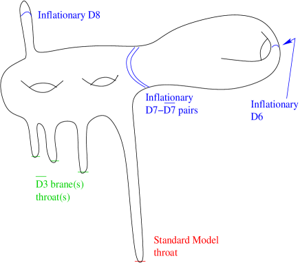
Figure 1: The general setup for our model is IIB string theory compactified in a warped CY as shown here. The warped CY has a complicated structure with several throats in which the warping is big and several other parts where the warping is milder. The SM is placed generically in one of the throats, but its precise embedding is not specified (also, the fact that it is on a throat is not crucial for the model to work). There are a series of anti D3s placed on throats as in the KKLT setup. Inflation is produced by one or several non-BPS systems like D6s wrapping toroidal 3-cycles, D7s-anti D7s on top of each other wrapping general cycles or D8s in the middle of KS throats. Presence of electromagnetic flux on these systems is generic.

2 Tachyon Inflation

In this section we will review the basic material needed to describe tachyon inflation in the presence of warping. We will start collecting some basic equations which will be needed later on.

2.1 Inflation Basics

In an effective field theory in 4d, slow-roll inflation is obtained if a scalar potential, $V(\phi)$, is positive in a region where the slow-roll conditions are satisfied:

$$\epsilon\equiv\frac{M_{pl}^{2}}{2}\ \left(\frac{V^{\prime}}{V}\right)^{2}\ \ll\ 1\ ,\ \ \ \ \qquad\eta\equiv M_{pl}^{2}\ \frac{V^{\prime\prime}}{V}\ \ll\ 1\ .$$ (1)

Where $M_{pl}$ is the rationalised Planck mass ($(8\pi G)^{-1/2}$) and primes refer to derivatives with respect to the scalar field, which is assumed to be canonically normalised. In the region where the slow-roll conditions are satisfied the scale factor suffers an exponential expansion $a\sim e^{Ht}$ with the number of e-foldings given by:

$$N(t)\equiv\int_{t_{init}}^{t_{end}}H(t^{\prime})dt^{\prime}\ =\ \frac{1}{M_{pl}^{2}}\int_{\phi_{end}}^{\phi_{init}}\frac{V}{V^{\prime}}\,d\phi\ .$$ (2)

A successful period of inflation required to solve the horizon problem usually needs at least $N\geq 60$. Slightly smaller values are allowed depending on the inflation scale.

The amplitude of density perturbations is given by :

$$\delta_{H}=\frac{2}{5}{\mathcal{P}}_{\mathcal{R}}^{1/2}=\frac{1}{5\pi\sqrt{3}}\,{V^{3/2}\over M_{pl}^{3}\,V^{\prime}}=1.91\times 10^{-5}\,,$$ (3)

where ${\mathcal{P}}_{\mathcal{R}}$ is the power spectrum computed in terms of the two-point correlators of the perturbations. The numerical value is given by the COBE normalisation which must be computed at the point where the last $60$ e-folds of inflation start. The spectral index is given by

$$n-1=\frac{\partial\ln{\mathcal{P}}_{\mathcal{R}}}{\partial\ln k}\simeq 2\eta-6\epsilon\,,\qquad\qquad{dn\over d\ln k}\simeq 24\epsilon^{2}-16\epsilon\eta+2\xi^{2}\,.$$ (4)

where $k$ is the length scale and $\xi^{2}\equiv M^{2}_{pl}\frac{V^{\prime}\,V^{\prime\prime\prime}}{V^{2}}$. This shows that for slow rolling ($\eta,\epsilon\ll 1$) the spectrum is almost scale invariant ($n\sim 1$).

2.2 Topological Inflation

Satisfying the slow-roll conditions is not an easy challenge for typical potentials since the inflationary region has to be very flat. Furthermore, after finding such a region we are usually faced with the issue of initial conditions, why should the field $\phi$ should start in the particular slow-roll domain.

Topological inflation was introduced in [38] partly as a way to ameliorate the issue of initial conditions of standard inflationary models. The idea is that usually starting the slow roll close to a maximum of a one-field potential is convenient because the corresponding parameter $\epsilon$ is naturally small there, leaving only the problem of finding a small enough $\eta$, which will be small enough if the maximum is very flat. But in general starting very close to this maximum is a very fine tuned configuration.

In topological inflation the initial conditions are governed by the existence of a topological defect at the maximum of a potential with degenerate minima. If the defect is thicker than the Hubble size $H^{-1}$, then a patch within the defect can inflate in all directions (including the ones transverse to the defect) and become our universe. The conditions for the thickness of the defect happen to be satisfied if the slow-roll condition, requiring $\eta$ to be small, holds. This is easy to see since the thickness of the defect ($\delta$) is inversely proportional to the curvature of the potential at the maximum which itself is proportional to $\eta$. Then, the condition $\delta\gg H^{-1}$ is satisfied if $\eta\ll 1$.

Topological inflation never ends, but the region that becomes our universe does so by standard rolling of the potential towards one of the minima, ending inflation once the slow-roll conditions cease to hold. Therefore this is a particular case of the standard slow-roll inflation and the topological defect only provides the natural initial conditions to start rolling close to the maximum. As such all the implications of small field inflation apply equally well here, including the spectrum of density perturbations. Notice that several inflationary potentials give rise to eternal inflation either due to quantum fluctuations or classical effects like in topological inflation (for a recent discussion of eternal inflation see [39]).

2.3 Tachyon Inflation

In a model with tachyon driven inflation, the starting point is a 4-dimensional effective action given by

$$S=\int\,d^{4}x\sqrt{-g}\left({M_{pl}^{2}\over 2}R-{\mathcal{A}}V(T)\sqrt{1+B\partial_{\mu}T\partial^{\mu}T}\right)+{\rm CS}\,,$$ (5)

where $M_{pl}$ is the 4-d Planck-mass, ${\mathcal{A}}$ and $B$ are positive dimensionless parameters which come from dimensionally reducing the effective action for an unstable probe brane system and usually depend on the metric warp factors, the string coupling $g_{s}$, string length $l_{s}=2\pi\sqrt{\alpha^{\prime}}$, the electric and magnetic flux that can be turned on in the world volume of the brane and the volume of the compact manifold. CS stands for the terms coming from the Chern-Simons part of the brane action. $V(T)$ is the tachyon potential which string field theory analysis suggests should be taken to be

$$V(T)={V_{0}\over\cosh({T\over\sqrt{2\alpha^{\prime}}})}\,.$$ (6)

Where $V_{0}$ is a dimension 4 parameter (in units of the string scale $m_{s}$) and it is proportional to $1/g_{s}$ and the volume of the cycle that the corresponding non-BPS brane is wrapping .

One considers a homogeneous tachyon field $T(x^{0})$ which acts as a perfect fluid source for gravity. Notice that the tachyon field $T$ in action (5) does not have canonical kinetic terms. We can define a canonically normalised field $\phi$ such that:

$$\phi\ =\ \sqrt{{\mathcal{A}}B}\int\sqrt{V(T)}\ dT$$ (7)

It is clear that expanding the square root in (5), the field $\phi$ will have canonical kinetic terms. It is with respect to $\phi$ that the slow-roll conditions apply. Using this relation between $\phi$ and $T$ we can rewrite the slow-roll conditions in terms of the field $T$ as follows:

$$\epsilon=\frac{M_{pl}^{2}}{2{\mathcal{A}}B}\ \left(\frac{V^{\prime 2}}{V^{3}}\right)\ \ll\ 1\ ,\ \ \ \ \qquad\eta=\frac{M^{2}_{pl}}{{\mathcal{A}}B}\ \left[\frac{V^{\prime\prime}}{V^{2}}\ -\ \frac{1}{2}\left(\frac{V^{\prime 2}}{V^{3}}\right)\right]\ll\ 1\ .$$ (8)

Prime now denotes differentiation with respect to $T$. Similarly, the number of e-foldings takes the form [31, 47]:

$$N(T)\approx\frac{{\mathcal{A}}B}{M_{pl}^{2}}\ \int_{T_{e}}^{T_{b}}{V^{2}\over V^{\prime}}\,dT\,,$$ (9)

where $T_{b}$ is the tachyon field value at the beginning of inflation and $T_{e}$ is the value at the end of inflation. The density perturbations take the following form in terms of the field $T$.

$$\delta_{H}\ =\ \frac{\sqrt{{\mathcal{A}}^{2}B}}{5\pi\sqrt{3}M_{pl}^{3}}\,\frac{V^{2}}{V^{\prime}}.$$ (10)

In the absence of warping, as argued in [7], in order to get many e-folds, one needs either a large string coupling or small compactification volume. In both cases, $\alpha^{\prime}$ corrections become very important and render the lowest order analysis incomplete and possibly wrong. Furthermore, it is clear that the tachyon potential does not have small parameters and cannot provide small values of $\epsilon$ and $\eta$, nor large values of $N$. The presence of the parameters ${\cal A}$ and $B$ makes the situation much better and amenable to analysis using the effective theory as argued in [31].

We can explicitly compute the slow roll parameters for the potential $V(T)$ in equation (6). This gives:

$$\epsilon=\frac{M_{pl}^{2}}{4\alpha^{\prime}{\mathcal{A}}BV_{0}}\ \frac{\sinh^{2}x}{\cosh x},\qquad\eta=-\frac{M_{pl}^{2}}{2\alpha^{\prime}{\mathcal{A}}BV_{0}}\ \cosh x\left[1-\frac{3}{2}\,{\rm{tanh}}^{2}x\right]$$ (11)

With $x\equiv\left(\frac{T}{\sqrt{2\alpha^{\prime}}}\right)$. It is now clear that for large enough values of ${\mathcal{A}}B$ the slow-roll conditions can be easily satisfied, giving rise to successful inflation. Notice that the scalar potential in terms of the canonically normalised field $\phi$ has a maximum at the origin with two minima at values of order $\sqrt{{\mathcal{A}}B}$ and therefore satisfies the conditions for topological inflation.

The number of e-foldings can be computed to be:

$$N\ \approx-\frac{2\alpha^{\prime}{\mathcal{A}}BV_{0}}{M_{pl}^{2}}\ \log\left(\frac{T_{b}}{\sqrt{8\alpha^{\prime}}}\right)$$ (12)

which can easily satisfy $N\geq 60$ for large enough warping ${\mathcal{A}}B$. The minus sign suggests that for the formula to be valid, $T_{b}<\sqrt{8\alpha^{\prime}}$. The density fluctuations can also be estimated to be

$$\delta_{H}=\sqrt{\frac{\alpha^{\prime}{\mathcal{A}}^{2}V_{0}^{2}B}{75\pi^{2}M_{pl}^{6}}}\,{\rm csch}\,\left(\frac{T_{b}}{\sqrt{2\alpha^{\prime}}}\right)$$ (13)

Choosing $T_{b}$ to correspond to the start of the last $60$ e-folds, we can easily satisfy the requirements $N=60$, $\delta_{H}=1.92\times 10^{-5}$ by adjusting three dimensionless parameters, namely ${\mathcal{A}}$, $B$ and the ratio $\gamma\equiv m_{s}/M_{pl}$ which itself depends on the volume of the extra dimensions and warp factors that will be explicitly defined in later sections. To get enough e-foldings (and satisfy slow-roll conditions) we need to have ${\mathcal{A}}B\gamma^{2}\sim 10^{2}$ and to satisfy the COBE normalisation we need ${\mathcal{A}}^{2}B\gamma^{6}\sim 10^{-10}$. These conditions can be satisfied very easily by properly choosing brane configurations, warped throats and moduli stabilisation at sufficiently large volume (in units of the string length). For instance ${\mathcal{A}}\sim 1$, $B\sim 10^{6}$ and $\gamma\sim 10^{-3}$ satisfy all the requirements, as well as ${\mathcal{A}}^{-2}\sim B\sim 10^{8}$, $\gamma\sim\left({\cal O}(10^{-2})-{\cal{O}}(10^{-1})\right)$. Notice that the factors ${\cal A}$, $B$ cannot be simultaneously large to satisfy both conditions. Therefore not every warped brane configuration will give rise to successful inflation . But some of them will.

This is very encouraging. However, one cannot choose the parameters ${\mathcal{A}}$ and $B$ arbitrarily as one needs to take into account the stabilisation of the volume of the compact manifold. In a realistic string model, the tachyon potential will depend on the dilaton and geometric moduli, which in the absence of other sources of potential, will have a runaway behaviour. Therefore, it is not consistent to concentrate only on the tachyon field dependence of the scalar potential in order to look for inflationary trajectories. Tachyon inflation should therefore be considered within a mechanism that fixes the moduli. Furthermore the choice of parameters has to be consistent with the effective field theory description in which the Kaluza-Klein masses have to be suppressed with respect to the string scale but larger than the Hubble scale. This will place strong restrictions on the choice as we shall see in the next sections, where we will describe these issues explicitly in the KKLT scenario of moduli stabilisation.

3 The Open-String Completeness Conjecture

One important observation at this stage is as follows. It has been known for a while [35, 32, 34] that the decay of an unstable brane will produce very massive closed string modes with masses comparable to $1/g_{s}$. These massive modes will back-react on the geometry potentially rendering the effective action analysis invalid. In order to take into account this back reaction, Sen has suggested an open-string completeness conjecture[35, 34] which we will review now.

According to the open-string completeness conjecture there is a quantum open string field theory that describes the full dynamics of an unstable D-brane without an explicit coupling to all the vibrational modes of the closed string. The classical results are supposed to correctly describe the evolution of the quantum expectation values in the weakly coupled open string field theory. The open string theory describes a consistent subsector of the full string theory and is capable of capturing the quantum decay process of an unstable D-brane. Although this conjecture has never been proved, there is strong evidence that it holds [35]. We will assume that this conjecture holds for the rest of the paper. This conjecture places constraints on the initial conditions that one can impose on the closed string fields in the effective action, for example the graviton. To demonstrate this let us review Sen’s analysis in [36]. There the starting point was the action in (5) with an additional cosmological constant term and with ${\mathcal{A}}=A_{0},B=1,M_{pl}=1$. For our analysis we will ignore this cosmological constant term as it will play no role to demonstrate the constraints following from the open-string completeness conjecture. Let us assume a spatially homogeneous time dependent solution in the FRW form:

$$T = T(x^{0})$$

$$ds^{2} = -(dx^{0})^{2}+a(x^{0})^{2}\left({dr^{2}\over 1-kr^{2}}+r^{2}d\theta^{2}+\sin^{2}\theta d\phi^{2}\right)\,,k=1\,.$$ (14)

The equations of motion for $a$ and $T$ that follow from (5) are

$${\ddot{a}\over a} = {A_{0}V(T)\over 6\sqrt{1-\dot{T}^{2}}}\left(1-{3\over 2}\dot{T}^{2}\right)\,,$$ (15)

$$3H{V(T)\dot{T}\over\sqrt{1-\dot{T}^{2}}}+\partial_{t}\left({V(T)\dot{T}\over\sqrt{1-\dot{T}^{2}}}\right) = -\sqrt{1-\dot{T}^{2}}V^{\prime}(T)$$ (16)

where $H=\dot{a}/a$ with the Friedman constraint

$$H^{2}={1\over 6}{A_{0}V(T)\over\sqrt{1-\dot{T}^{2}}}-{1\over a^{2}}\,.$$ (17)

Once the Friedman constraint is satisfied at an initial time, it is satisfied at all times since its time derivative leads to the equations of motion (16). For the two second order differential equations, we need four initial conditions. The Friedman equation imposes one constraint. One can choose the origin of time by imposing $\dot{T}=0$ at $x^{0}=0$ thereby eliminating an additional condition. Thus we are left with two possible initial conditions. Naively one would take these to be $T(x^{0})=T_{0}$ and $\dot{a}(x^{0})=a_{0}$. The open string completeness conjecture reduces this two-parameter space of solutions to a one-parameter family of solutions. This is done by noting that the rolling tachyon solution describing the decay of a D-brane in open string theory is time reversal symmetric. Thus the solutions following from the above equations of motion must also be time reversal symmetric. For this to be possible, we must choose $a(x_{0})=a(-x_{0})$ thereby imposing $\dot{a}=0$ at $x_{0}=0$. Note that this implies that solutions with a big-bang singularity will also have a big-crunch. Sen found time reversal symmetric solutions in [36], however he found that the slow-roll conditions could not be met and hence sufficient number of e-folds could not be obtained. We will perform a more detailed analysis motivated by this in a KKLT inspired scenario and include the effects of warping which would impose $B\neq 1$ and also introduce warp factor dependence in $A$. In our simple model we will also include a Kähler moduli to study what happens to the compact manifold during this period of cosmological evolution of our universe. We will find that in our models getting sufficient number of e-folds excludes the scenario of big-bang-big-crunch.

4 Non-BPS D-branes and Flux Compactification

4.1 Dimensional reduction of flux compactification

Type IIB string compactifications on Calabi-Yau orientifolds with three-form fluxes have a flux-induced warped metric [48] . It can be written as:

$$ds^{2}=e^{2\omega-6u+6u_{0}}\bar{g}_{\mu\nu}dx^{\mu}dx^{\nu}+e^{-2\omega+2u}\tilde{g}_{mn}dy^{m}dy^{n}$$ (18)

where the 4d spacetime coordinates are $x^{\mu}$, $\mu=0,1,2,3$ whereas the internal space coordinates are $y^{m}$ $m=4,\cdots 9$. Here $\omega(y)$ is a function of the internal coordinates of the manifold that defines the warp factor, and $u(x)$ is a four-dimensional field corresponding to the real part of the Kähler modulus that determines the volume of the compact space. We will suppose that the internal metric has only one Kähler modulus (whose imaginary part is $e^{4u(x)}$) and a number of complex structure moduli. $u_{0}$ is a dimensionless constant whose magnitude will be fixed afterwards. After dimensional reduction, all the complex structure moduli and the dilaton get fixed to its value at some minimum of the potential derived from the GVW superpotential [49, 48] generated by the flux of the complex type IIB form $G_{3}$. We will consider all the excitations of these complex structure moduli fields to have been consistently integrated out from four dimensional physics. The four dimensional action reads then [51]

$$S={M_{pl}^{2}\over 2}\int d^{4}x\sqrt{-\bar{g}}\left[\bar{R}-24(\bar{\nabla}u)^{2}\right]$$ (19)

with

$${M_{pl}^{2}\over 2}={e^{6u_{0}}\over(2\pi)^{7}g_{s}^{2}\alpha^{\prime 4}}\int d^{6}y\sqrt{-\bar{g}}~{}e^{-4\omega(y)}.$$ (20)

Being a supersymmetric construction, this action can be put in terms of a Kähler potential and a superpotential. If we define the Kähler modulus to be $\rho(x)\equiv Y(x)+iX(x)$, with $X(x)\equiv e^{4u(x)}$, and the axion field $Y$ is defined from the RR 4-form $C_{(4)}$. Then the four dimensional action (19) becomes (where an appropriate kinetic term for $Y$ has been added)

$$S={M_{pl}^{2}\over 2}\int d^{4}x\sqrt{-\bar{g}}\left(\bar{R}-6{\bar{\nabla}_{\mu}\bar{\rho}\bar{\nabla}^{\mu}\rho\over|\rho-\bar{\rho}|^{2}}\right)$$ (21)

that has the canonical form for a ${\cal N}=1$ supergravity action with Kähler potential $K=-3~{}{\rm log}[-i(\rho-\bar{\rho})]$. From now on, we will assume the field $Y(x)$ to be stabilised at some minimum (we will be more concrete in the following sections) and suppose its fluctuations to decouple from the spectrum at low energies.

The vev of $X$ is related to the value of the volume of the compact dimensions. This volume is given by

$${\rm Vol}_{6}=\int d^{6}y\sqrt{g_{6}}=\langle X\rangle^{3/2}\int d^{6}y\sqrt{\tilde{g}}~{}e^{-6\omega}$$ (22)

4.2 Dimensional reduction of the tachyon action

Consider the following (string frame) action for the non-BPS D$p$-brane in Type IIB string theory ($p$ even). This action is also valid for a $D\bar{D}$ system where the branes are sitting on top of each other and with no world-volume gauge field turned on, in which case one has to change $T_{p}\to\sqrt{2}T_{p}$.

$$S_{T}=-T_{p}\int_{M_{4}\times\Sigma}d^{p+1}x\,V(T)\sqrt{|g_{ab}+\partial_{a}T\partial_{b}T|}$$ (23)

The change from the string frame to the Einstein frame is given by a change in the metric of the form $g_{\mu\nu,E}=e^{\phi_{0}-\phi}g_{\mu\nu,s}$, where $\phi_{0}$ is the vev of the dilaton [52]. In the Einstein frame the tension of the Dp brane reads

$$T_{p}={\sqrt{2}(2\pi)^{-p}\alpha^{\prime-{{p+1}\over 2}}\over g_{s}}.$$ (24)

For $T(x)$ only depending on time and assuming that the warping is only transverse to the brane , we finally find

$$S_{T,DBI} = -\sqrt{2}(2\pi)^{-p}\alpha^{\prime-{p+1\over 2}}g_{s}^{-1}h_{p-3}\tilde{\cal V}^{2}\times$$

$$\times \int d^{4}x\sqrt{|\bar{g}|}e^{(p-15)u}e^{(7-p)\omega(y_{p})}V(T)\sqrt{1-e^{-2\omega+6u-6u_{0}}\,\dot{T}^{2}}$$

where $\omega(y_{p})$ stands for the value of $\omega(y)$ in the position of the brane. We have assumed $|\bar{g}^{00}_{E}|=1$, that is what we are going to find hereafter. We have moreover defined

$$h_{p-3}\equiv\int d^{p-3}y\sqrt{|\tilde{g}_{int}|}.$$ (26)

This factor will depend on the Calabi-Yau under consideration; we will see examples below of its value in several scenarios. We can consistently add this action to (19) provided that the addition of this term can be seen as the addition of a D-term. This can be argued by noting that the 32 bulk supersymmetries are non-linearly realised in the world-volume for the non-BPS branes.

4.3 The 4D potential for the Kähler modulus

We can add a potential term for $u$ following KKLT, but we must argue that these non-perturbative corrections will not mix with the tachyon. A heuristic argument for this is as follows. Non-perturbative corrections arise from evaluating the partition function at Euclidean saddle points. For a finite contribution, one needs a finite action for an Euclidean object which then gets exponentiated. In the KKLT set up the Euclidean object under consideration is a D3 brane which wraps a 4-cycle of the compact manifold. If one added an anti-D3 brane, it could annihilate this D3 brane if it wrapped the same 4-cycle as a result of which the non-perturbative potential would need to get modified by a function that depended on the position of the anti-D3 brane. Such a complication will not arise in the cases that we will consider. In principle, however, euclidean non-BPS D$p$ branes could wrap some cycle of the compact manifold and produce a finite action which would add to the non-perturbative superpotential. Such contribution would look like

$$C(T)\,e^{-b(T)X^{(p+1)/4}}\,,$$

with $C(T)\rightarrow 0$ as the tachyon condenses. Since $p+1>6$ in the cases where we get inflation, such terms will not contribute. Furthermore we envision the non-BPS brane generating the tachyon potential to be separated from the four-cycles where the gauge theory generating the non perturbative superpotential sits.

The four dimensional action for a single chiral multiplet $\rho$ is given by

$$S={M_{pl}^{2}\over 2}\int d^{4}x\sqrt{-\bar{g}}\left(\bar{R}-g_{\rho\bar{\rho}}\bar{\nabla}_{\mu}\rho\bar{\nabla}^{\mu}\bar{\rho}-V_{F}(\rho)\right)+({\rm D-terms})$$ (27)

with $g_{\rho\bar{\rho}}=\partial_{\rho}\partial_{\bar{\rho}}K$, $g^{\rho\bar{\rho}}=(g_{\rho\bar{\rho}})^{-1}$ and $D_{\rho}W=\partial_{\rho}W+W\partial_{\rho}K$, and

$$V_{F}(\rho)={M_{pl}^{2}\over 2\pi}e^{K}\left[g^{\rho\bar{\rho}}D_{\rho}W\overline{D_{\rho}W}-3|W|^{2}\right]$$ (28)

is the standard F-term part of the supergravity scalar potential. Let us then assume a KKLT-like superpotential for $\rho$ (remember we are going to use $e^{4u}={\rm Im}\rho$)

$$W=W_{0}+De^{ic\rho}$$ (29)

The field $Y$ in $\rho$ can be easily stabilized at $\langle Y\rangle=\pi$ and integrated out, so that $\rho=\pi+iX$. This yields , using $K=-3{\rm log}(-i(\rho-\bar{\rho}))$

$$V_{F}={M_{pl}^{2}\over 2\pi}{cDe^{-cX}\over 2X^{2}}\left({1\over 3}\,cDXe^{-cX}-W_{0}+D\,e^{-cX}\right)$$ (30)

This potential has a supersymmetric minimum. We can add, following KKLT, a set of anti D3-branes breaking supersymmetry in the form of a D-term in another throat. The action for an anti-D3 brane is

$$S_{\overline{D3}}=-T_{3}\int d^{4}x\sqrt{|g_{4}|}=T_{3}\int d^{4}x\sqrt{|\bar{g}|}e^{4\omega(y_{i})}e^{-12u}=T_{3}\int d^{4}x\sqrt{|\bar{g}|}e^{4\omega(y_{i})}X^{-3}$$ (31)

$y_{i}$ specifies the position of the anti D-brane $i$ in the CY. These anti-D3s are attracted to the tip of the throat and prefer to sit there. There $e^{4\omega(y_{i})}\sim X~{}{\rm exp}(-{8\pi K\over 3g_{s}M})$, where $M$ and $K$ specify the RR and NSNS fluxes turned on in the throat. The whole effect is to add the potential (30) a term like

$$\delta V={E\over X^{2}}$$ (32)

with

$$E={2\over M_{pl}^{2}}T_{3}\sum_{i}e^{-{8\pi K_{i}\over 3g_{s}M_{i}}}=(2\pi)^{-3}\alpha^{\prime-2}g_{s}^{-1}\sum_{i}e^{-{8\pi K_{i}\over 3g_{s}M_{i}}}$$ (33)

Note that the potential $V_{\rm total}=V+\delta V$ scales as $\mu^{3}V_{\rm total}$ under

$$D\rightarrow\mu^{3/2}D,\quad W_{0}\rightarrow\mu^{3/2}W_{0},\quad E\rightarrow\mu^{3}E\,,$$ (34)

keeping the minimum unchanged. Other interesting scaling property of $V_{\rm total}$ is that under the change

$$D\rightarrow\lambda^{3/2}D,\quad W_{0}\rightarrow\lambda^{3/2}W_{0},\quad E\rightarrow\lambda^{2}E,\quad c\rightarrow\lambda^{-1}c\,,$$ (35)

the potential is invariant provided that $X\to\lambda X$, that is, the whole structure of extrema gets shifted horizontally. One can investigate a wider parameter space using these scaling properties. Furthermore, for bigger $W_{0}$ one should take into account the $\alpha^{\prime}$ corrections. We will put in the first $\alpha^{\prime}$ correction that comes from the $R^{4}$ term in IIB [54, 55, 56, 57]. This is given by

$$V_{\alpha^{\prime 3}}={9\sqrt{5}\xi\mu^{3}W_{0}^{2}\over 4\sqrt{2}X^{9/2}}\,,$$ (36)

where $\xi=-\chi(M)\zeta(3)\alpha^{\prime 3}/(16\pi^{3})$, $\chi(M)$ being the Euler number of the compact manifold. We choose $\xi\approx 1$ although one can easily accommodate other choices allowing for larger $\xi$.

4.4 Summarising: The total 4D action

Putting all these pieces together we find (we will assume that $u$ only depends on the time coordinate)

$$S = {M_{pl}^{2}\over 2}\int d^{4}x\sqrt{-\bar{g}}\left(\bar{R}_{4}+24(\dot{u})^{2}-\hat{V}(u)\right)$$

$$-(2\pi)^{-p}\alpha^{\prime-{p+1\over 2}}g_{s}^{{p-3\over 4}}h_{p-3}e^{(15-p)u_{0}}\times$$

$$\times\int d^{4}x\sqrt{|\bar{g}|}e^{(p-15)u}e^{(7-p)\omega(y_{p})}V(T)\sqrt{1-e^{-2\omega+6u-6u_{0}}\dot{T}^{2}}$$

with

$${\hat{V}}(X) \equiv V_{F}+\delta V+V_{\alpha^{\prime 3}}$$ (38)

$$= {\mu^{3}M_{pl}^{2}\over 2\pi}{cDe^{-cX}\over 2X^{2}}\left({1\over 3}cDXe^{-cX}-W_{0}+De^{-cX}\right)+{E\over X^{2}}+V_{\alpha^{\prime 3}}\,,$$

where we have explicitly put in the scaling parameter $\mu$ and $X\equiv e^{4u}$. Notice that the full potential as a function of $X$ and $T$ can be written (in the small kinetic energy approximation for the tachyon) as:

$$V_{total}(X,T)\ =\ \hat{V}(X)\ +V_{tachyon}\,.$$ (39)

5 Four dimensional effective action and inflation

5.1 Friedman equation

Consider the following 4D action (we will later substitute the actual values of the parameters but we will leave them as parameters in order not to lose generality:

$$S={M_{pl}^{2}\over 2}\int d^{4}x\sqrt{-g}\left\{R-2\Lambda-\beta(\partial u)^{2}-\hat{V}(u)-AV(T)\sqrt{1+B(\partial T)^{2}}\right\}$$ (40)

With the standard FRW ansatz for the metric (14) we get the following equations of motion for the metric, assuming a homogeneous ansatz $T(x)=T(x^{0})$ and $u(x)=u(x^{0})$,

$$H^{2} = {1\over 3M_{pl}^{2}}\rho-{k\over a^{2}}\,,$$ (41)

$${\ddot{a}\over a} = -{1\over 6M_{pl}^{2}}\left(3p+{\rho}\right)\,,$$ (42)

where

$$\rho = {M_{pl}^{2}}\left\{\Lambda+{1\over 2}\beta\dot{u}^{2}+{1\over 2}\hat{V}(u)+{1\over 2}{A\cdot V(T)\over\sqrt{1-B\dot{T}^{2}}}\right\}\,,$$ (43)

$$p = {M_{pl}^{2}}\left\{-\Lambda+{1\over 2}\beta\dot{u}^{2}-{1\over 2}\hat{V}(u)-{1\over 2}A\cdot V(T)\sqrt{1-B\dot{T}^{2}}\right\}\,.$$ (44)

5.2 Summary, values for the parameters and initial conditions

Including the equations of motion for $X\equiv e^{4u}$ and $T(t)$, we find the following system of equations:

$$3H{AVB\dot{T}\over\sqrt{1-B\dot{T}^{2}}}+\partial_{t}\left({ABV\dot{T}\over\sqrt{1-B\dot{T}^{2}}}\right) = -A\sqrt{1-B\dot{T}^{2}}~{}V^{\prime}(T)$$ (45)

$$\beta\partial_{t}\left({\dot{X}\over 4X}\right)+{3\beta H\dot{X}\over 4X}+2X\partial_{X}\hat{V}(X)+2X\partial_{X}\left(AV(T)\sqrt{1-B\dot{T}^{2}}\right)=0$$ (46)

$${\ddot{a}\over a}=-{1\over 3}\beta\left(\dot{X}\over 4X\right)^{2}+{1\over 6}\hat{V}(X)+{A\cdot V(T)\over 6\sqrt{1-B\dot{T}^{2}}}\left({1-{3\over 2}B\dot{T}^{2}}\right)$$ (47)

with $\hat{V}(X)$ given in equation (38). Comparing (4.4) to (40), the values of the parameters are

$$\beta = 24$$ (48)

$$A = {2\sqrt{2}\over M_{pl}^{2}}(2\pi)^{-p}\alpha^{\prime-{(p+1)\over 2}}g_{s}^{-1}e^{(7-p)\omega(y_{p})}X^{(p-15)\over 4}\tilde{\cal V}^{2}h_{p-3}$$ (49)

$$B = {e^{-2\omega(y_{p})}X^{3/2}\over\tilde{\cal V}}$$ (50)

$$E = {2\over M_{pl}^{2}}(2\pi)^{-3}\alpha^{\prime-2}\sum_{i}e^{-{8\pi K_{i}\over 3g_{s}M_{i}}}$$ (51)

where we have defined

$${\cal V}=\tilde{\cal V}\int d^{6}y\sqrt{\tilde{g}}e^{-4\omega(y)}\equiv\tilde{\cal V}C\alpha^{\prime 3}\\$$ (52)

with $\tilde{\cal V}=e^{6u_{0}}\equiv X_{0}^{3/2}$ and so

$$\alpha^{\prime}={2\tilde{\cal V}C\over g_{s}^{2}(2\pi)^{7}M_{pl}^{2}}.$$ (53)

$c$, $D$, $W_{0}$ are taken to be the values in [20], except for a minus sign in $W_{0}$ that cancels out the effect of taking $\langle Y\rangle=\pi$: $c=0.1$, $D=1$, $W_{0}=1/25000$. However, we will make use of scaling properties of the potential (34), (35) to explore a wider space of parameters.

Up to this point all the analysis has been model independent; the differences among models will depend in the concrete value of $h_{p-3}$ as well as in the dependence of the warping and the compactification volume on the parameters of the model. We will analyse this issues in detail in the forthcoming sections.

There are other factors that can change the value of $A$ and $B$ in a rather model independent way: these are the electric and magnetic flux one can turn on the world volume of the brane, and the external, constant NSNS $B$ field that can be consistently added to any model without spoiling the GKP/KKLT construction. We will briefly review these issues in the section 6.

5.3 The particular case of $D9-\overline{D9}$ pairs

We show in this section why it is impossible to get inflation with the $D9-\overline{D9}$ system if one does not provide extra sources of tension to the branes, such as electromagnetic fluxes. The action for the $D9-\overline{D9}$ system in the absence of these extra sources is

$$S={2\sqrt{2}\over M_{pl}^{2}}T_{9}\int d^{10}x\sqrt{g_{MN}+\partial_{M}T\partial_{N}T}.$$ (54)

Using the general metric metric (18) and expanding inside the square root one finds

$$A\simeq{g_{s}\over 2\pi^{2}\alpha^{\prime}}{\int d^{6}y\sqrt{\tilde{g}}~{}e^{-2\omega}\over\int d^{6}y\sqrt{\tilde{g}}~{}e^{-4\omega}},\quad\quad B\simeq{\int d^{6}y\sqrt{\tilde{g}}~{}e^{-4\omega}\over\int d^{6}y\sqrt{\tilde{g}}~{}e^{-2\omega}}.$$ (55)

It follows that the number of e-folds is

$$N\simeq\alpha^{\prime}AB\simeq{g_{s}\over\sqrt{2}\pi^{2}}.$$ (56)

5.4 Applying the open-string completeness conjecture

We have three second-order coupled differential equations for $X$, $T$ and $a$. We need six initial conditions. Now, Sen’s open string completeness conjecture puts a constraint on the form of the tachyon equation (45). This equation has been derived from a four dimensional action, that has in turn been derived from a ten dimensional effective action where the tachyon field is invariant under the symmetry $x_{0}\to-x_{0}$ as dictated by conformal field theory analysis. This implies that all the effective physics regarding the tachyon has to be invariant under this symmetry. In particular, equation (45) has to be. The easiest and most natural way to fulfil this requirement is to set

$$T(x_{0}) = T(-x_{0})$$

$$X(x_{0}) = X(-x_{0})$$ (57)

$$a(x_{0}) = a(-x_{0})$$

Note that these conditions preserve the time translational symmetry $x_{0}\to x_{0}\to x_{0}+h$, since e.g. $T(x_{0}+h)=T(-x_{0}-h)$. This and (57) imply that $\partial_{t}f(t)|_{t=0}=0$, for $t=x_{0}+h$ and $f=T,u,a$. As we see, Sen’s completeness conjecture is putting constraints on the initial conditions:

• We have the freedom to choose the origin of time, that is, $h$ above. We set $h=0$.

• This automatically implies, by Sen’s conjecture,

  $$\dot{a}(0)=\dot{T}(0)=\dot{X}(0)=0$$ (58)

• Friedman’s equation puts another constraint in the equations of motion:

  $$H^{2} = {1\over 6}\beta\left(\dot{X}\over 4X\right)^{2}+{1\over 6}\hat{V}(X)+{1\over 6}{A\cdot V(T)\over\sqrt{1-B\dot{T}^{2}}}-{k\over a^{2}}.$$ (59)

  This has to be valid at all times. However, the time derivative of this equation is the equation of motion for $a(t)$, and, since this is a first order differential equation, the constraint is valid for all times if imposed at $t=0$. Then, we have the initial condition

  $${1\over 6}\hat{V}(X(0))+{1\over 6}A\cdot V(T(0))-{k\over a(0)^{2}}=0$$ (60)

  All the solutions we are going to consider are such that $\hat{V}(X(0)),V(T(0))>0$, and thus we must set $k=1$.

So we have fixed four initial conditions in (58), (60) out of the six initial ones. Eq. (60) fixes the value of $a(0)$ in terms of $T(0)$ and $X(0)$.

Now, we can fix the value of $X(0)$ demanding that it stays in the value that minimises the potential (in absence of tachyon) in $t=0$. Given that $X(t)$ is going to be symmetric with respect to the time and it is going to move all the time around this minimum, we can consider this to be (approximately) its value at the beginning of time. With respect to $T(0)$, it is usually argued that the initial value of the inflaton field should be close to 1 in Planck units. Assuming this to be true, and following (7), the initial value of $T$ should be chosen to be of order 0.1.

5.5 Evolution of the system

Before we proceed putting numbers in the system, we find it convenient to give an overview of the dynamics of the system.

We want to consider the tachyon to be the only field driving inflation, whereas the volume modulus field remains as a constant. The tachyon field evolution is given by equation (45) whereas its coupling to the metric is given by (47). We can decouple the modulus field from the system supposing $\dot{X}=0$ and $\hat{V}(X_{min})=0$, in order for the cosmological constant not to drive inflation. If we manage to get dynamically $\dot{X}=0$, then we can use the results of [31, 47] to study the tachyon evolution in a slow-rolling regime.

To consider the stabilisation of the field $X$, first we have to be careful that $A$ is sufficiently small for the total potential at $t=0$, $\hat{V}(X)+A(X)V(T_{0})$ has a minimum different from $X=\infty$. This necessary condition can be rephrased in terms of an approximate inequality between the Hubble constant during inflation and the gravitino mass first derived in [59]

$$H\lesssim m_{3/2}.$$ (61)

Once we have chosen $A$ to fulfil this property we must set the initial value of $X$ in the minimum (or near the minimum) of the total potential $\hat{V}+AV(T_{0})$. Note that this minimum will not be exactly the same of the KKLT potential. We discuss the naturalness of such a choice in section 7. The contribution of the tachyon potential to the total potential for $X$ starts to decrease as time grows, and $X$ will undergo small damped oscillations (since the minimum starts displacing towards the KKLT minimum). These oscillations will quickly stop due to the damping and the possible relevance of them to density perturbations are completely negligible since they occur just at the beginning of inflation.

Inflation happens while the tachyon stays close to the maximum of its potential. Once the tachyon abandons this maximum inflation quickly ends. The potential for $X$ decreases from the initial value to the KKLT potential, and $X$ undergoes a displacement from its original minimum to the KKLT minimum.

Another interesting issue is the behaviour of the system under a rescaling of the form (34). It should be noted that, once the condition (61) is fulfilled, one can make $W_{0}$ as big as one wants (but being careful to evaluate all the relevant $\alpha^{\prime}$ corrections) since the inflation is driven by $A$ (and the residual cosmological constant left over after the KKLT mechanism) while $X$ is at the minimum of the potential. However, the bigger $W_{0}$ is, the higher the fine tuning one has to make in considering the initial value of $X$ to get inflation and not decompactification. For acceptable values of $W_{0}$, as those considered along the paper, no fine tuning in the initial position of $X$ is necessary.

A last remark is in order. In order to trust our effective description for the fields different from $T$ it is necessary that, for all times, $m_{s}\geq m_{KK}\geq H$. This is in principle non trivial since the value of $m_{s},m_{KK}$ will depend on the warping in a sensitive way. The open string scale in the inflationary throat in units where $M_{pl}=1$ is roughly given by

$$m_{s}^{2}\sim{1\over B\alpha^{\prime}}\,.$$ (62)

In order to see this, note that the tachyon mass sets the string scale. Expanding the tachyon potential to leading order and rescaling the tachyon field to canonical form leads to the above result. Note that $B$ depends on warping and hence the string scale in this instance is suppressed. The Kaluza-Klein open string scale is set by

$$m_{KK}^{2}\sim{1\over BV_{3}^{1/3}}\,,$$ (63)

where $V_{3}$ is the volume of the 3-cycle that the D6-brane wraps around. Since the warp factor does not depend on the world-volume directions we can choose $V_{3}$ to be greater than ${\cal O}(\alpha^{\prime})$ and make $m_{KK}<m_{s}$. Note that the closed string scale and the closed string Kaluza Klein scale involve the averaged warp factor and are in principle bigger than the above scales. Moreover, the decay of the D-brane will give rise to massive closed string modes, but the open-string completeness conjecture allows us to average their effect by taking into account the initial conditions.

In the numerical analysis performed in the following section we have found ${\cal O}(m_{s})\gg{\cal O}(H)$, where we have used formula (62) for $m_{s}$. This was possible by turning on a world-volume near critical electric field which reduces the Hubble scale as to be explained in the next section.

It could be argued that in scenarios in which ${\cal O}(m_{s})\sim{\cal O}(H)$ a non-negligible density of primordial black holes could be produced. While, in accordance with the completeness conjecture the dynamics of the closed string black holes should be captured by the classical evolution of the field $T$, quantum fluctuations of $T$ could give rise to primordial open string black holes (not necessarily limited to the beginning of inflation), whose fast decay could leave a trace on the CMB. Such result would necessarily depend on the exact relation between $m_{s}$ and $H$ and then its study lays far beyond the scope of this paper.

6 Addition of electric, magnetic and NS-NS B-fields

As stressed above, the addition of electric and/or magnetic in the world volume of the branes, or, alternatively, constant NS-NS B-field in the bulk, can significantly enhance the phenomenological features of a given model. Setting them to zero is too restrictive. Let us briefly review how these fields can affect the inflationary scenario. The DBI action takes the general form:

$$S_{T}=-T_{p}\int_{M_{4}\times\Sigma}d^{p+1}x\,V(T)\sqrt{|g_{ab}+Q_{ab}+\partial_{a}T\partial_{b}T|}$$ (64)

Where $Q_{ab}=B_{ab}+2\pi\alpha^{\prime}F_{ab}$, with $B_{ab}$ the bulk NS-NS antisymmetric tensor field and $F_{ab}$ is the gauge field strength.

6.1 Electric field

To illustrate the effect of an electric field on the physical parameters $A$ and $B$, let us consider the simple case when the 6-d metric is flat. Let us turn on an electric field along an internal direction labelled by $m$ which is consistent with the symmetries of the FRW metric. In this case the $p+1$ dimensional Lagrangian for the non-BPS brane takes the form

$$A_{p}V(T)\sqrt{g_{4}}\sqrt{1-B\dot{T}^{2}-E^{2}}\,.$$ (65)

The equation of motion for $E$ is given by

$$\partial_{m}{\sqrt{g_{4}}A_{p}V(T)E\over\sqrt{1-B\dot{T}^{2}-E^{2}}}=0\,,$$ (66)

This tells us that if $g_{4}$, $A_{p}$ and $B$ are independent of the internal coordinate $m$ then a constant $E$ will satisfy this equation. This is true for example when the 6-d space is a torus. In this case the 4-d effective Lagrangian can be rewritten as

$$\hat{A}V(T)\sqrt{g_{4}}\sqrt{1-\hat{B}\dot{T}^{2}}\,,$$ (67)

where $\hat{A}=A\sqrt{1-E^{2}}$ and $\hat{B}=B/(1-E^{2})$. Thus the total number of e-folds which is proportional to $AB$ would increase. This is consistent with the fact that tachyon condensation is supposed to slow down in the presence of a background electric field as shown in [63]. Also we see that this can reduce the Hubble scale keeping the string scale fixed and hence can be useful in adjusting the scales in the analysis.

For the case of a KS geometry, things are more complicated since the 6-d metric will introduce a dependence on $m$ generically. As a result a constant $E$ solution will no longer be valid. One could however presumably choose $E$ in a coordinate and time-dependent manner that improves the number of e-folds and it would be interesting to investigate this issue further.

6.2 Magnetic field

If we turn on a constant magnetic field in the internal dimension, this will effectively change the Lagrangian to

$$AV(T)\sqrt{1-B\dot{T}^{2}}\sqrt{g_{int}+F_{int}}\,,$$ (68)

as a result it is easy to see that this leads to effectively increasing $A$ keeping $B$ unchanged. Since the magnetic field has a topological nature, one must have 2-cycles in the wrapped region to be able to turn on this field in a consistent way.

6.3 Constant NS-NS B-field

One could also consider turning on a background constant $B_{0m}=e$, where $m$ labels an internal dimension. In this case the Lagrangian of the probe non-BPS brane takes the form

$$AV(T)\sqrt{1-B\dot{T}^{2}-Be^{2}}\,,$$ (69)

as a result by tuning $Be^{2}$ close to 1, we could reduce $A\rightarrow A\sqrt{1-Be^{2}}$ while increasing $B\rightarrow B/(1-Be^{2})$. This in principle could lead to sufficient number of e-folds while satisfying density perturbation and spectral index constraints.

Thus we see that having a background $B_{0m}$ field potentially can resolve problems with tachyon inflation. Also note that since $A$ is reduced, this lowers the Hubble scale while keeping the string scale fixed. As to be explained in the discussion this can resolve a potential problem with scales in tachyon driven inflation models.

6.4 Issues concerning the addition of fluxes

One could wonder whether the addition of electric or magnetic field can leave some trace (apart from the trace left by the decay of the brane without fluxes) in the CMB after tachyon condensation. In the case of the magnetic field the answer is clearly no: magnetic field corresponds to the presence of lower dimensional non-BPS branes in the world-volume of the corresponding non-BPS state, and they will produce the same kind of topological defects as the mother non-BPS brane does. The case of the electric field is more complicated since after tachyon condensation a density of fundamental strings are left over stretching in the same direction of the original electric field [63]. This happens in particular if the original electric field was turned on in a homotopically non-trivial cycle and is not expected if the cycle is trivial.

Another interesting issue is that of the fine tuning. While in the concrete models we have analysed a large amount of magnetic flux seems to be needed to obtain phenomenologically acceptable results (though this situation might not be generic), this cannot be interpreted as fine tuning. However, in the case of the electric field it turns out that one must choose $E^{2}\to 1$ in $\hat{A}$, $\hat{B}$ in order to make its contribution relevant. While from the numerical point of view it seems an undeniable fine tuning, a more careful study of the physical problem shows that a $E$ is not a sensible parameter to describe the electric field, but rather $\tilde{f}\equiv{E\over\sqrt{1-E^{2}}}$, since it is the integral of this field (the conjugate momentum of $A_{i}$) over an sphere at infinity what yields the electric charge. Thus, a value of $E$ very close to 1 should not be interpreted as fine tuning since this interpretation only relies on a bad choice of variables. This interpretation cannot be given for the NSNS field, in which case a value of this field very close to 1 should be interpreted as fine-tuning.

7 Example 1: Klebanov-Strassler throat

Although one can perform a general analysis of the equations (45)-(47) for an arbitrary CY (assuming that there always exists some CY such that the values of $A$ and $B$ computed from its geometry satisfy all the phenomenological requirements), we find it interesting to analyse in detail the scenario in concrete geometries.

We consider in this section an illustrative example of a warped region of a Calabi-Yau which corresponds to a deformed conifold. We will see that it is very difficult to satisfy the slow-roll conditions for inflation in this case. In the next section we consider a more successful example.

The warped deformed conifold solution of Type IIB sting theory, also known as Klebanov-Strassler throat [64], is one of the few known CY metrics. A detailed study of its geometry has been carried out in [65, 66]; we refer to these papers to the interested readers.

The KS geometry once embedded in a general CY manifold has two 3-cycles that are dual to each other; the metric and fluxes are a good solution of Type IIB supergravity provided that $M$ units of RR 3-form flux $F_{3}$ are turned on on the $S^{3}$ three-cycle that is on the tip of the throat and $-K$ units of NSNS $H_{3}$ flux are turned on in the dual 3-cycle:

$${1\over(2\pi)^{2}\alpha^{\prime}}\int_{A}F=M;\hskip 56.9055pt{1\over(2\pi)^{2}\alpha^{\prime}}\int_{B}H=-K$$ (70)

where $A$ is the $S^{3}$ and $B$ its dual 3-cycle. The complete metric is very well known and analysed, but for our purposes let us just say that there are two interesting limits in the geometry. The first one is the geometry ’far from the tip of the throat’, that is valid for large radial coordinate $r$. In this case the metric has the approximate form

$$ds_{10}^{2}=e^{6u_{0}-6u}{r^{2}\over R^{2}}d\bar{s}_{4}^{2}+e^{2u}{R^{2}\over r^{2}}(dr^{2}+r^{2}ds_{T^{1,1}}^{2}).$$ (71)

where $T^{1,1}$ is a 5-dimensional space with the topology of $S^{2}\times S^{3}$. $R$ is a dimensionful quantity given by

$$R^{4}={27\over 4}\pi g_{s}MK\alpha^{\prime 2}.$$ (72)

The other interesting limit is the tip of the throat, that is a 7-dimensional manifold (the volume of the $S^{2}$ in $T^{1,1}$ has been shrunk to zero size) with metric

$$ds_{7}^{2}=e^{2\omega-6u+6u_{0}}d\bar{s}_{4}^{2}+e^{2u}\tilde{R}^{2}ds_{S^{3}}^{2}.$$ (73)

where $\tilde{R}$ and $e^{2\omega}$ are given by

$$\tilde{R} = \sqrt{g_{s}M}~{}\alpha^{\prime 1/2}$$ (74)

$$e^{2\omega} = e^{-{4\pi K\over 3g_{s}M}}.$$ (75)

Let us now discuss several ways of realising our scenario in the KS geometry.

7.1 D6-branes localised on the tip of the throat

The metric in which we must embed the brane is (73), which is of the form (18) for $\tilde{g}_{mn}=e^{2\omega}\tilde{R}^{2}g_{mn,S^{3}}$. Now, in this case $h_{3}=2\pi^{2}\tilde{R}^{3}e^{3\omega}$. If we substitute this value for $h_{3}$ in (49), (50), we find (after fixing the volume modulus)

$$A = {4\sqrt{2}\pi^{3}e^{4\omega}\alpha^{\prime-1}g_{s}^{5/2}\over X_{0}^{3/4}C}$$ (76)

$$B = e^{-2\omega}.$$ (77)

Now, note that [17]

$$C=k\left({2\pi\over 3}\right)^{3}\left({27\pi\over 4}g_{s}MK\right)^{3/2}$$ (78)

for $k\geq 1$ some real number. The number of e-folds becomes (evading again fine tuning of $T_{0}$, like in previous section)

$$N\simeq\alpha^{\prime}AB={27\over\sqrt{2}}\left({4\over 27\pi}\right)^{3/2}{g_{s}e^{-4\pi K\over 3g_{s}M}\over kK^{3/2}X_{0}^{3/4}}$$ (79)

that is, at most, a number of order $10^{-2}$. Note that we cannot make this number any better by turning on electric or magnetic fields since there are no 1-cycles or 2-cycles in a $S^{3}$. This situation resembles the giant inflaton case studied in [17].

7.2 Branes wrapping $T^{1,1}$, away from the tip.

The case of the non-BPS $D8$ admits an interesting variation on the scenario. One can consider wrapping the D8 in a 5 cycle of $T^{1,1}$ with the topology of $S^{2}\times S^{3}$ at a value of $r$ different from zero. While this system dynamically tries to go to the tip of the throat where it annihilates into the vacuum, one can consider the interesting possibility of turning on a magnetic flux along the directions of the $S^{2}$. This magnetic field is topological and takes values in the integers over the area of the 2-cycle. After pullbacking the KS metric in the world volume of the brane in the presence of magnetic flux, it is easy to see that a potential for the position of the brane is generated, that stabilises it away from the tip where the 2-cycle shrinks to zero. This magnetic field would then have the dual role of stabilising the brane far from the throat and enhancing the number of e-folds. Note that the same comments might apply for $D5-\overline{D5}$ pairs wrapped in the $S^{2}$ away from the tip. A detailed investigation of this scenario may deserve further study.

7.3 Branes along the throat, wrapping the $r$ direction

We can consider $D6$ or $D7-\overline{D7}$ pairs wrapping the $r$ direction and one of the 2- or 3-cycles available in the KS geometry. For this to make sense, the complete KS metric should be used. However, for the sake of illustration we will use the simplified form of the metric (71), from a infrared cutoff $r_{0}\ll R$ to $R$, where the throat is supposed to merge with the whole CY.

The DBI action for a brane wrapping the $r$ direction after volume stabilisation is

$$S_{DBI}={2T_{p}\over M_{pl}^{2}}\int d^{4}x\sqrt{-\bar{g}}~{}\Omega_{p-3}X_{0}^{p-3\over 4}V(T)\int dr~{}R^{p-7}r^{3}\sqrt{1-{R^{2}\over r^{2}}\dot{T}^{2}},$$ (80)

where $\Omega_{p-3}$ is a numerical factor coming from the angular integration. Considering the case of very big warping at the tip of the throat, $e^{-2\omega}=e^{{4\pi K\over 3g_{s}M}}\gg 1$, we find (for $R^{2}\dot{T}^{2}/r^{2}$ small)

$$\int_{r_{0}}^{R}dr~{}R^{p-7}r^{3}(1-{R^{2}\over 2r^{2}}\dot{T}^{2})\simeq{R^{p-3}\over 4}(1-\dot{T}^{2}),$$ (81)

where we have assumed $r_{0}\ll R$. The values of the $A$ and $B$ parameters is (using (78))

$$A = (2\sqrt{2}){(2\pi)^{7-p}\alpha^{\prime(7-p)/2}g_{s}\Omega_{p-3}X_{0}^{p-9\over 4}R^{p-9}\over 4k\left({2\pi\over 3}\right)^{3}}$$ (82)

$$B = 2.$$ (83)

The factor of $(\sqrt{2})$ appears in the $D7-\overline{D7}$ case. The number of e-folds is given by

$$N=(\sqrt{2}){27~{}(2\pi)^{4-p}\over 2k}\Omega_{p-3}X_{0}^{p-9\over 4}\left({27\pi\over 4}MK\right)^{p-9\over 4}g_{s}^{p-5\over 4}.$$ (84)

Note that this number is again something of order $10^{-1}$, what makes it difficult to reconcile with the cosmological observations.

8 Example 2: D6 branes in $T^{3}$ fibres

As a second model, consider the case of wrapping a non-BPS D6 brane in a 3-cycle of the CY with the topology of a torus. These cycles are quite generic, since following the work of Strominger, Yau and Zaslow [67], every Calabi-Yau that has a mirror is expected to be a $T^{3}$ fibration over some basis. Let us see how we can combine this topological statement with the GKP setup in order to perform a quantitative analysis of inflation in such a setting.

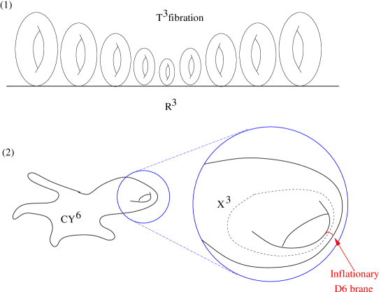
Figure 2: Depiction of the CY as a $T^{3}$ fibration. (1) Locally, the CY can be seen as a $T^{3}$ fibration over ${\bf R}^{3}$. (2) The global structure of the CY can be very complicated but one can envisage that locally one can have D6 branes wrapped in the $T^{3}$ fibre at the point of maximum warping. Here $X^{3}$ represents the (3 dimensional) local base space.

Our aim then is to consider in the GKP setup a construction that is locally ${\bf R}^{3}\times\tilde{T}^{3}$, with $\tilde{T}^{3}$ is a warped torus (warping in the directions of ${\bf R}^{3}$). The metric in the vicinity of that region is of the form

$$ds^{2}=Z^{-1/2}d\bar{s}_{4}^{2}+e^{2u_{0}}Z^{1/2}({\rm d}\vec{\bf x}^{2}+{\rm d}\vec{\bf y}^{2})$$ (85)

where $\vec{\bf x}$ are the coordinates in the ${\bf R}^{3}$ patch and $\vec{\bf y}$ are the coordinates in the $T^{3}$ fibre. Let us assume that $Z$ does not depend on $y$. The equation of motion for the warping function $Z(x)\equiv e^{-4\omega}$ reads

$$(\tilde{\nabla}^{2}Z){\rm vol}=g_{s}F_{3}\wedge H_{3}$$ (86)

with ${\rm vol}=\sum dx_{i}\wedge dy_{i}$, the volume form of the (unwarped) internal manifold, and the $\tilde{\nabla}^{2}$ refers to the Laplacian in the internal unwarped coordinates. We can wrap the RR $F_{3}$ flux along the $T^{3}$ directions and the NSNS $H_{3}$ flux along the dual directions ($X_{3}$ in figure 7). Dirac quantisation conditions imply roughly that

$$F_{3} = {M\over V_{T^{3}}}$$ (87)

$$H_{3} = {K\over V_{X^{3}}}.$$ (88)

with $K$, $M$ integers. ISD condition for the fluxes will imply that

$${M\over V_{T^{3}}}={K\over V_{X^{3}}}$$ (89)

with $V_{X}^{3}$, $V_{T^{3}}$ the corresponding volumes in $\alpha^{\prime}$ units, and these numbers $M$, $K$ have to satisfy a tadpole condition of the form

$$MK\lesssim 10^{4}.$$ (90)

The solution of (86) will be of the form

$$e^{-2\omega(x)}=Z^{1/2}(x)\simeq g_{s}^{1/2}\sqrt{{M\over V_{T^{3}}}{K\over V_{X^{3}}}}|x|.$$ (91)

There will be in principle other dependences in $x$ as well as integration constants; one should remark at this point that (86) is not the complete equation but it has some contribution from point-like charges like O3s and D3s that we will consider to be far apart from our solution. The complete solution will be unique and will fix all the arbitrariness of (91). Let us assume that $x\sim 1$, $V_{X^{3}}\sim 1$, $V_{T^{3}}\sim 1$. This will imply, after moduli stabilisation

$$B=e^{-2\omega}=g_{s}^{1/2}(KM)^{1/2}.$$ (92)

Now, $A$ is given in the D6 case by

$$A={g_{s}\sqrt{2}(2\pi)^{7-p}e^{(7-p)\omega}X_{0}^{p-9\over 4}\alpha^{\prime{(1-p)\over 2}}\over C}h_{p-3}={2\pi\sqrt{2}g_{s}^{3/4}\over\alpha^{\prime}k(KM)^{3/4}X_{0}^{3/2}},$$ (93)

where we have used the fact that $C=\int e^{-4\omega}\sqrt{\tilde{g}}\sim k(KM)$ for $k$ some positive real number greater than 1, $h_{3}=\alpha^{\prime 3/2}V_{T^{3}}/X_{0}^{3/4}$ and we have chosen $V_{T^{3}}\sim 1$. It is quite clear that one will not get a sufficient number of e-folds just will these $A$ and $B$. The addition of $n$ units of magnetic flux will increase $A$ by a factor of $n/$Area, where Area is the area in $\alpha^{\prime}$ units of the $T^{2}$ inside $T^{3}$ where we turn on this magnetic field. We can consider this area to be of order 1. In addition, we can consider a value for the electric field $f\equiv{1\over\sqrt{1-E^{2}}}$ as a time-varying Wilson line along one of the 1-cycles of the $T^{3}$. After all this we get

$$A={2\sqrt{2}\pi ng_{s}^{3/4}\over\alpha^{\prime}fk(KM)^{5/4}X_{0}^{3/2}},\quad B=f^{2}g_{s}^{1/2}(KM)^{1/2}$$ (94)

Can we satisfy the constraints for the number of e-folds and the density perturbations for some values of these parameters? The number of e-folds in absence of fine-tuning for the initial value of the tachyon field is roughly given by

$$N\simeq\alpha^{\prime}AB\simeq 10^{2}$$ (95)

and the density perturbations are given by

$$\delta_{H}^{2}={1\over 25\pi^{2}}{H^{4}\over p+\rho}={(2\pi)^{7}\over 300\pi^{2}}{\alpha^{\prime 2}g_{s}^{2}\over X_{0}^{3/2}C~{}{\rm sinh}^{2}({T_{0}\over\sqrt{2\alpha^{\prime}}})}A^{2}B.$$ (96)

The phenomenological constraints (number of e-folds and density perturbations) amount to have, in terms of the parameters of the model

$$N\simeq\alpha^{\prime}AB\simeq{2\sqrt{2}\pi nfg_{s}^{5/4}\over k(KM)^{3/4}X_{0}^{3/2}} \simeq 10^{2}$$ (97)

$$\delta_{H}^{2}\simeq{(2\pi)^{9}\over 300\pi^{2}}{2g_{s}^{4}n^{2}\over k^{3}(KM)^{3}X_{0}^{9/2}} \simeq 10^{-10}$$ (98)

both constraints can be easily satisfied with standard values for the parameters like $g_{s}\sim 0.1$, $M\sim K\sim 10$, $kX_{0}^{3/2}\sim 10^{3}$, $n\sim 10^{3}$, $f\sim 10^{4}$. This implies a large volume of the compactification manifold ($\sim 10^{6}-10^{7}$ in units of $\alpha^{\prime}$), consistently with having all the sources far away from the toroidal construction, and also a somewhat large electric and magnetic flux. Many other combinations of these parameters may also give the desired values.

9 Results

9.1 Inflation by non-BPS $D6$ brane

Here we present numerical results for inflation generated by a non-BPS D6 brane, in order to show explicitly how the dynamical evolution of the system proceeds and to illustrate graphically issues like moduli stabilisation, the end of inflation and the big crunch-big bang transition. It is more convenient to work in units where $M_{pl}=1$. We will assume that the numbers for $A$ and $B$ can be adjusted by turning on a combination of bulk fluxes and world-volume fluxes. The initial conditions and values for various parameters are as follows:

$$E = 3.9\times 10^{-12}$$

$$A = 2\times 10^{-3}X^{-9/4}\,,\quad B=5\times 10^{9}\left({X\over X_{min}}\right)^{3/2}$$

$$c = 0.1\,,\quad~{}~{}~{}~{}\,D=1$$

$$\quad W_{0} = {1\over 25000}\,,\quad T(x^{0}=0)=0.1\,,$$ (99)

with the rescaling parameters

$$\mu=800,\quad\lambda=1,$$

so that the effective $W_{0}\approx 0.9$. We have chosen $E$ and $\Lambda$ so that the minimum for $\hat{V}(X)$ is of ${\cal O}(10^{-16})$ at $X_{min}=124.636$. This is because we do not want inflation to be driven by the cosmological constant term We have also conducted separate numerical tests with a more fine-tuned $E$ such that the minimum is even lower and have obtained very similar results. Including the contribution from the tachyon, the effective potential takes the shape of the thinner line in figure 2.

Figure 3: Effective potential with and without tachyon contributions. The thicker line shows the potential at the end of tachyon condensation while the thinner is the potential at the beginning.

Note that the initial potential has a minimum as well. This property is crucial to prevent decompactification from happening. The behaviour for the number of e-folds and $a(t)$ as a function of time are exhibited in figure 3. Using the parameters specified above, we get around 90 e-folds.

Figure 4: Number of e-folds vs $t$ and $a(t)$ vs $t$.

We have displayed the time reversal property of $a(t)$ explicitly. Other important quantities such as the volume of the compact manifold, tachyon potential, $\rho+3p$ are demonstrated below. We will not display $t<0$ explicitly in these graphs although it should be assumed that the solution is time symmetric.

Figure 5: $X(t)$ vs t and $\rho+3p$ vs $t$.

Figure 6: $V(T)$ vs $t$.

Finally, we have plotted the deviation of the spectral index from unity as a function of the number of e-folds. This has the behaviour given in figure 6.

Figure 7: Plot of $n-1$ vs $N$

We have used the formulae

$${\cal P}(N) = {1\over 25\pi^{2}}{H^{4}\over p+\rho}$$ (100)

$$n-1 = {d\ln{\cal P}(N)\over dN}$$ (101)

$$\delta_{H} = \sqrt{{\cal P}(N)}|_{N=30}\,.$$ (102)

This suggests that the spectral index is between $0.95$ and $0.96$. However, this value can be pushed closer to unity by making $AB$ larger. We have also estimated the density perturbation and found it to be $\approx 2\times 10^{-5}$ at $N\approx 30$. We choose $N=30$ since the COBE normalisation has to be imposed at approximately 60 e-foldings before the end of inflation. Since the total number of e-foldings is 90 in this example, we calculate the spectral index and the density perturbation when $N=30$. One can perhaps tune the parameters to make these results better. In this model, the energy scale during inflation is $H\approx 10^{14}$ GeV. Also the amplitude of gravitational waves produced during inflation is $h\approx{H\over M_{p}}\lesssim 10^{-5}$ which satisfies observational constraints on CMB anisotropy. One can potentially get the same physics as in our example in models with large extra dimensions as in [57]. This is very interesting and merits further investigation.

9.2 Fine-tuning in our models

The usual drawback of inflationary models is the huge amount of fine tuning required to make the model work. We have argued that our model suffers less from fine tuning than other inflationary models, particularly stringy ones. The reasons are two-fold. First the warp factor dependence in the non-BPS D-brane action. This warp factor depends on the fluxes and therefore can take relatively large values. This includes the electric and magnetic fluxes. The explicit models that we have require large volume and large 3-form and magnetic fluxes. We then exchange fine-tuning by large fluxes. Notice that in the successful cases of $T^{3}$ fibrations, the warping of the metric induced by the fluxes is not exponential. The second reason is that the tachyon field is not subject to the standard $\eta$ problem of supergravity potentials since its 4d action is not manifestly supersymmetric.

We can still check how much fine-tuning is needed for the parameters of our model. We have numerically verified that small variations of the values we have chosen give rise to small variations in the number of e-folding, and as expected any reduction of the number of e-foldings can be compensated by the choice of the warp factors.

10 Discussion and Outlook

Let us finish with a discussion of some relevant issues of our scenario:

• General bounds on scales in any tachyon driven inflation model

  We saw that the string scale is given by ${c\over B\alpha^{\prime}}$ where $c$ is an unknown constant. The Hubble scale is given by ${AV\over 6}$. In order for the string scale to be bigger than the Hubble scale we need

  $${c\over B\alpha^{\prime}}>{AV\over 6}\,.$$ (103)

  Using the formula for the number of efolds and denoting the integral $\int_{T_{e}}^{T_{b}}{V^{2}\over V^{\prime}}dT=\Delta/\alpha^{\prime}$, we have

  $$6c>{NV\over 2\Delta}\,.$$ (104)

  Thus for $c\sim O(1)$ we find that $\Delta$ has be quite large which is only possible if the tachyon was sitting very close to the top of the potential and if $AB\sim O(1)$. However, this immediately leads to the problem that $\eta\propto{1\over AB}\sim O(1)$ and thus we are not in the slow-roll regime any more. Although the number of e-folds can be quite large, the density perturbation constraints will no longer be satisfied. There are two possible resolutions to this impasse. Firstly, $c$ could be larger. With $c$ of $O(10)$ the numerical example in the paper would yield a string scale twice as large as the Hubble scale. Secondly, one could turn on a world-volume electric field which will reduce the Hubble scale keeping the string scale fixed. This in principle will make the scales work in the right direction. Notice that these constraints allow a large number of e-folds but not arbitrarily large.

• Time reversal symmetry of the solutions

  All our cosmological solutions are invariant under a change $t\to-t$. This kind of solution arise from the evolution of the open-string field $T$ that describes (following Sen’s conjecture) the decay of the non-BPS object only if the initial conditions allow for this time-reversal symmetry of the system. This does not imply that more general, time asymmetric solutions cannot exist: it implies that such solutions cannot be described in such a simple way, with the tachyonic action 5.

  Time reversal symmetry implies that if the universe is to end up in a big crunch singularity for $t=t_{0}$, then it must have started from a big bang singularity in $t=-t_{0}$. Analogously, if the fate of the Universe is to expand forever at $t\to\infty$, it is because it started from an infinitely extended initial state in $t\to-\infty$. In this sense, we must clarify what we understand by big bang. In order to get a proper understanding of the situation, we should identify the big bang to be the state of the universe at $t=0$.

  Note that in our model the universe can never be singular at $t=0$, since following equation (60) $a(0)>0$. This (non singular) big bang is always a consequence of a previous (non singular) big crunch, note that the null energy condition of [58] that forbade big crunch-big bang transition does not apply here since here $k=1$.

• Exit from inflation

  The fact that we are able to track the system for all time relies heavily on Sen’s conjecture. By studying the (classical) evolution of a open string field we are actually considering all the complicated interactions of the set of closed string fields produced during the decay. It is the conjecture what allows us to trust the effective theory for all times and what allows us to put numbers in the end of inflation.

  With respect to a mechanism for reheating, we assume that a mechanism like that proposed in [23] applies. The SM is supposed to be placed in the tip of a throat whose warping is much bigger than that of the inflationary throat (see figure 1). In this case, the graviton wave-function is peaked in the SM throat and the closed string modes produced during the decay can serve (enhanced by the gravitational blue-shift) to excite the SM degrees of freedom.

  In any case, a complete study of the problem of reheating is beyond the scope of this paper.

• (De)compactification and Big Crunch singularity

  The evolution of the system presents the following peculiarity. If the initial ($t=0$) value of $X$ is such that its potential energy is much bigger than the KKLT barrier, during its evolution it will overshoot KKLT barrier and the universe will undergo decompactification. If this decompactification is fast enough, then

  $${\ddot{a}\over a}\simeq-\left(\dot{X}\over 4X\right)^{2}$$ (105)

  very soon and the four dimensional space is led to a big crunch singularity. In these cases, The usual damping term for the scalar field given by $H$ is very small or even negative, thus not disturbing (or even enhancing for $H<0$) the decompactification process. On the other hand, if the $t=0$ conditions are such that $X$ is trapped inside the KKLT well, it will always be there (since its evolution suffers from a damping term) and stabilises very soon. Then it is a good approximation to consider it as a constant for all times, while the four dimensional universe inflates.

  We have however found some marginal cases in which the position of $X$ is tuned so that it overshoots the barrier with very little kinetic energy and thus its slow-rolling evolution turns on inflation of the four dimensional universe, producing at the same time decompactification. However, the amount of inflation obtained in this way is always very small compared to the case with the volume modulus stabilised. Moreover, these cases are very marginal and one has to fine tune the position of $X$ to get such a behaviour.

  Another case that leads to decompactification and big crunch are those with a very big initial value of $T$. In this case, tachyon decay proceeds very fast and the closed string moduli starts to oscillate. These oscillations are negligibly damped and, after some time, get enhanced by a negative value of $H$, what asymptotically leads to decompactification plus big crunch.

  We find, then, in a broad majority of cases, either inflation with moduli stabilised or decompactification with big crunch.

  We are tempted to conclude that, since such KKLT potentials (with a set of metastable vacua and then a runaway behaviour for an infinite vev of the moduli fields) are supposed to be generic in string theory, such a behaviour of change of roles between compact and non-compact dimensions under cosmological evolution is quite generic, independently of the model of inflation considered. This seems to agree with recent studies [61].

• $\alpha^{\prime}$-corrections

  Although we took the first $\alpha^{\prime}$-correction for the superpotential into account, there are also potential corrections to the tachyon effective action. Not much is known about these. Suppose there were terms in the effective action of the form $((\partial_{\mu}\partial^{\mu})^{n}T)^{2k}$. Since the contraction of the indexes is with $e^{-2\omega}/Vg^{\mu\nu}$, it is quite possible that there is an enhancement compared to the unwarped case (where these terms are volume suppressed) unless the higher tachyonic derivatives are vanishingly small. Although this is true during slow-roll, this is not necessarily true during the period of exit from inflation as our graphs show. Thus these terms, if present, could become very important during this phase. Taking them into account in a systematic manner is beyond the scope of this paper. However, these terms will not alter the conclusion that sufficient number of e-folds can be produced with the tachyon as the inflaton. Furthermore, we have checked numerically that in our models, $e^{-2\omega}\ddot{T}/V<<1$ as a consequence of which we believe that our results may correctly capture the physics even towards the end of inflation.

In summary, we have presented a successful inflationary scenario in string theory with moduli stabilization. We made progress in obtaining inflation in a natural way by controlling the amount of fine tuning in terms of the flux-induced warp factors. It is worth mentioning that the exponentially warped regions such as the Klebanov-Strassler geometry turned out to be less suitable to satisfy the slow-roll conditions. Whereas regions with no exponential warping, such as the $T^{3}$ fibrations, can give rise to inflation, requiring large volume and fluxes. Therefore we exchange the fine tuning of parameters needed in other string inflation models by the introduction of large fluxes. The slow-roll conditions are not satisfied by $D9-{\overline{D9}}$ systems unless magnetic fluxes could be included. They are also difficult to satisfy for $D6$ branes on KS throats. $D8$ and $D5-{\overline{D5}}$ may satisfy them once magnetic fluxes are included. The most concrete successful example we provided was for $D6$ branes on $T^{3}$ fibrations. We also expect similar conditions for $D7-{\overline{D7}}$ systems wrapping on four-cycles with non-trivial two-cycles inside. A detailed study of all these configurations lies outside the scope of this article.

Our scenario also opens new avenues to explore string cosmology in flux compactifications. The implications of the open-string completeness conjecture have proved very efficient to extend the model to earlier regions of the universe, leaving interesting possibilities for speculation about the initial conditions.

There are many open questions remaining that would need further attention. We have made several simplifying assumptions to keep the model as simple as possible. In particular we have assumed that the complex structure moduli and the dilaton have been stabilised and only concentrated on the Kähler structure modulus/ tachyon system. In the same way that the tachyon dependence alters the potential for $X$ during the brane decay time, it may also affect the other moduli. In both cases there is a dependence on these fields of the tachyon part of the potential. The dilaton dependence can be seen by tracing the $g_{s}$ factors of $V(T)$ in the total scalar potential. The complex structure moduli associated to the size of the three-cycle that the D6 brane is wrapping, would also appear in the tachyon potential. It would be interesting to follow the cosmological evolution of all these fields also but this is beyond the scope of this article. We may argue that in the absence of the non-BPS brane the dilaton is fixed at weak coupling, and since its potential blows-up at infinity, then the coupling to the tachyon gives rise to only a runaway dependence (recall that the dilaton field $\tau$ is such that Im($\tau)\propto 1/g_{s}$) that may change only slightly the cosmological evolution of $\tau$. We hope to address this issue in the future.

Also, recently [56, 57], an extension of the KKLT scenario has been put forward such that the potential stabilises at an exponentially large volume, with all other moduli also fixed. The coupling of these systems, that require at least two complex structure moduli, to the tachyon may lead to interesting cosmological implications. The exponentially large volume is welcome in order to better trust the effective field theory description.

Finally, we have compared our scenario with the brane-antibrane and racetrack inflation, especially regarding the advantages on fine tuning and initial conditions. It may also be possible to consider different stages of inflation in which several of these mechanisms may be at work at different times in the evolution of the universe.

To conclude, some words about the physical interpretation of time-reversible situations. Clearly, the time symmetry of this scenario asks for a proper interpretation of the full cosmological scenario. At the moment we can say that starting from $t=0$, the evolution of the universe is just like in standard eternal topological inflation, driven in this case by the decay of a non-BPS brane. We may consider if there is any physical meaning at all regarding the $t<0$ region of our spacetime. Notice that the initial condition $\dot{T}=0$ is different from the finite velocity assumed in the S-brane interpretation of the tachyon potential [62]. Unlike that case, our scenario is completely time-symmetric: in a sense, there is no preferred arrow of time. The case $v=0$ of [62] would correspond to $T(0)=0$ in our case (that is a classically static situation), while our general case has not any analog along the lines of [62] (note that for $T(0)\neq 0$ the tachyon never reaches the top of the potential). It would be interesting to develop a full cosmological picture based on our results.