Energy Landscape of d-Dimensional Q-balls

Abstract

We investigate the properties of $Q$-balls in $d$ spatial dimensions. First, a generalized virial relation for these objects is obtained. We then focus on potentials $V(\phi\phi^{\dagger})=\sum_{n=1}^{3}a_{n}(\phi\phi^{\dagger})^{n}$, where $a_{n}$ is a constant and $n$ is an integer, obtaining variational estimates for their energies for arbitrary charge $Q$. These analytical estimates are contrasted with numerical results and their accuracy evaluated. Based on the results, we offer a simple criterion to classify “large” and “small” $d$-dimensional $Q$-balls for this class of potentials. A minimum charge is then computed and its dependence on spatial dimensionality is shown to scale as $Q_{\rm min}\sim\exp(d)$. We also briefly investigate the existence of $Q$-clouds in $d$ dimensions.

I Introduction

Many physical systems may be efficiently modeled in a reduced number of spatial dimensions. In particular, certain static solutions of nonlinear partial differential equations exhibiting solitonic behavior, or at least spatial localization, have been shown to exist from hydrodynamics and condensed matter physics h-cm to relativistic field theories rel . At the opposite extreme, the possibility that the four fundamental interactions of nature may be unified in theories with extra spatial dimensions has triggered a search for static nonperturbative higher-dimensional solutions of a variety of models derived from string theory stringy-sol . The extra dimensions may be compact and much smaller than the usual three dimensions of space, as in Kaluza-Klein models KK , or they may be infinitely large, as in the recent Randall-Sundrum scenario, where gravity (and, possibly, other fields) can leak into one or more dimensions orthogonal to the 3-dimensional brane where matter and gauge fields propagate and interactRS .

In either higher-dimensional formulation, there is plenty of motivation to search for $d$-dimensional nonperturbative configurations with $Q$ quanta. The reasons are two-fold: first, as an upsurge of recent work suggests, it is possible that these extra dimensions may be much larger than the planckian scale Antoniadis ; Csaki . If the fundamental gravity scale is $M$, the associated length scale of the extra dimensions is $R_{\rm KK}\simeq(M_{\rm Pl}/M)^{2/(d-3)}M^{-1}$. [$d-3\geq 1$ is the number of extra dimensions.] Thus, if $M\sim 1$ TeV, $R_{\rm KK}\sim 10^{32/(d-3)}10^{-17}$ cm. For $d\geq 5$, this scenario is still acceptable by current tests of Newton’s gravitational law Rubakov . In this case, it is possible that signatures of extra dimensions may be discovered in collider experiments Antoniadis ; Giudice ; Quiros . For example, energy may leak out into the bulk, disappearing from three dimensional space (missing energy) or, more relevantly for the present work, higher dimensional solitonic configurations may be produced at future accelerators, as has been recently suggested by one of us d-oscillons . Thus, computing their properties, such as energy and spatial extension, and how they scale with spatial dimensionality, is of great interest: if the fundamental interactions giving rise to the observed configuration are known, their properties may serve as a probe to determine the dimensionality of spacetime d-oscillons . Another reason for considering such objects is that they may well exist in a pre-compactification spacetime. Being nonperturbative, they may contribute in as yet unknown ways to the compactification process or even to the stability of the compactified internal space. Their existence may change the structure of the vacuum, a possibility worth exploring in the near future.

In the present work we will focus on a particular class of nonperturbative configurations called $Q$-balls. This choice reflects the fact that they are – as will be shown – the simplest static, spatially-localized configurations that can be found in any number of spatial dimensions. They have been shown to appear in many versions of 3-dimensional field theories, supersymmetric or not (see references in next paragraph) and will most certainly be present in their higher-dimensional extensions, although we will not present a detailed study of specific examples here. As in the early work concerning 3-dimensional $Q$-balls, our strategy is to start by studying their properties in the simplest possible models that can support them. More specific applications are the next logical step. $Q$-balls are non-dissipative, spatially-localized scalar field configurations that owe their stability to the conservation of a global charge $Q$ Coleman . As such, they belong to the general class of nontopological objects constructed to bypass the limitations imposed by Derrick’s theorem forbidding the existence of static localized configurations of real scalar fields in more than one spatial dimension Derrick . The distinguishing feature of $Q$-balls is that they can be constructed from a single complex scalar field; most nontopological solitons are built out of two or more interacting scalars Lee .

Since they were first proposed by Coleman, these objects have triggered many different avenues of research: some searched for $Q$-balls in nonabelian models nonabelian or with several interacting fields gaugeQ , others in supersymmetric models susyQ and the effects of their mutual interactions interacQ , while others investigated their stability against quantum effects Graham and their cosmological role cosmoQ . Understandably, this past work was confined to the usual three spatial dimensions. Given the recent upsurge of interest in higher-dimensional theories, we believe it important to investigate how the properties of $Q$-balls depend on spatial dimensionality. Although there is a trend to consider models with compactified extra dimensions, in this work we will consider only $Q$-balls in flat $(d+1)$-dimensional Minkowski spacetimes. One reason is that these objects will typically have radii $R_{Q}$ which are much smaller than the scale of the compactified space, $R_{KK}$, in particular in the context of models with large extra dimensions Antoniadis ; that is, they will “see” a flat $d$-dimensional space.

Our emphasis throughout this work is to explore how spatial dimensionality affects some of the key properties of $Q$-balls: their energy, minimal charge, and size. For this purpose, we will employ a combination of analytical and numerical tools, often contrasting one with another.

The paper is organized as follows. In section 2 we present the class of models we will be working with, establishing notation and definitions. We also obtain a $d$-dimensional virial relation for $Q$-balls that is shown to encompass Derrick’s theorem when $Q=0$. In section 3, we define the type of potentials we will be using throughout this work and study large $Q$-balls, using a variational ansatz for their spatial profiles to estimate their energies and explore some of their properties. We contrast our results with numerical computations. In section 4 we treat small $Q$-balls, again using a variational approach. We show that the concept of “small” $Q$-ball makes more sense for lower dimensional models, as dimensionality greatly affects the minimum charge for these objects. We obtain an analytical estimate for the minimum charge $Q_{\rm min}$ as a function of spatial dimension $d$ accurate for $d\leq 6$, and find a simple relation, $Q_{\rm min}\sim\exp[d]$. In section 5 we briefly explore the existence of $Q$-clouds in $d$ dimensions. $Q$-clouds are unstable diffuse solutions of the equations of motion discovered by Mark Alford a few years after Coleman first published his paper Q-clouds . We were unable to find $Q$-clouds for $d\geq 6$, $d=5$ being marginal. We close in section 6 presenting our conclusions and plans for future work.

II $Q$-ball Basics and $d$-Dimensional Virial Theorem

II.1 Basics

Consider a scalar field $\phi$ with Lagrangian density

$${\cal L}=\partial_{\mu}\phi^{\dagger}\partial^{\mu}\phi-V(\phi\phi^{\dagger})~{},$$ (1)

where $\mu=0,1,...,d$ and the metric is $\eta_{\mu\nu}={\rm diag}(1,-1,-1...)$. We will restrict our analysis to models with a conserved $U(1)$ symmetry.

The potential $V(\phi\phi^{\dagger})$ is assumed to have a global minimum at $\phi=0$. $Q$-balls are nonperturbative excitations about this global vacuum state carrying a conserved charge $Q$, the net particle number. Thus, if the energy of the $Q$-ball, $E_{Q}$, is smaller than $Qm_{\phi}$ [$m^{2}_{\phi}=V^{\prime\prime}(0)$ is the mass of (perturbative) particle-like vacuum excitations at $\phi=0$], $Q$-balls are stable and energetically preferred. This is an example of nonperturbative effects dominating the physics of the vacuum. If a model supports such configurations, one cannot claim to understand the physics of the vacuum before incorporating their contribution. Configurations with lowest energy are obtained by writing Coleman ; Lee

$$\phi({\bf x},t)=\frac{1}{\sqrt{2}}\Phi({\bf x})e^{i\omega t}~{}.$$ (2)

From the associated conserved current $j^{\mu}=-i(\phi^{\dagger}\partial^{\mu}\phi-\phi\partial^{\mu}\phi^{\dagger})$, one obtains the charge conservation law,

$$Q=\omega\int d^{d}x\Phi^{2}~{}.$$ (3)

In practice, $Q$-balls are very similar to critical bubbles in the theory of homogeneous nucleation or, to use Coleman’s expression, false vacuum decay falsevacuum . The latter is characterized by an asymmetric double-well potential, with the field initially trapped in the false vacuum state. The critical bubble or bounce is the spherically-symmetric static solution to the equation of motion that interpolates (or almost) between the two potential minima: at $r=0$, $\phi(r=0)\equiv\phi_{c}$ is close to the global minimum $\phi_{+}$ and, as $r\rightarrow\infty$, it approaches the false vacuum at $\phi=0$. The field configurations for $Q$-balls do the same. But how could this be if the potential $V$ has a global and not a local minimum at $\phi=0$? The answer, a clever trick, comes from the term in the equation of motion proportional to $\ddot{\phi}\propto-\omega^{2}\Phi$. This term contributes an effective negative mass to the potential: for certain choices of $\omega$, it makes the minimum at some $\phi_{+}$ the global minimum and the minimum at $\phi=0$ the false vacuum. One can see this by varying the action obtained from the Lagrangian in eq. 1 using the form of the field of eq. 2 to obtain,

$$\nabla_{d}^{2}\Phi=-\omega^{2}\Phi+\frac{\partial V}{\partial\Phi}\equiv U^{\prime}(\Phi)~{}.$$ (4)

The particle “moves” in the effective potential $-U(\Phi)$. As $\omega\rightarrow m_{\phi}$ the barrier separating the two minima disappears and the vacuum at $\phi=0$ becomes classically (spinodally) unstable.

II.2 Virial Theorem

From the Lagrangian density of eq. 1 and using eq. 2, we obtain the energy for a field configuration in $d$ spatial dimensions as

$$E[\Phi]=\int d^{d}x\left[\frac{1}{2}(\nabla_{d}\Phi)^{2}+\frac{1}{2}\omega^{2}\Phi^{2}+V(\Phi^{2})\right]~{}.$$ (5)

We can use eq. 3 to express the energy in terms of the conserved charge $Q$,

$$E_{Q}[\Phi]=\frac{1}{2}\frac{Q^{2}}{\langle\Phi^{2}\rangle}+\langle\frac{1}{2}(\nabla_{d}\Phi)^{2}\rangle+\langle V\rangle~{},$$ (6)

where $\langle\dots\rangle\equiv\int\dots d^{d}x$. Now scale the spatial variable $x\rightarrow\alpha x$ and impose that the energy is invariant under scale transformations, $\partial E/\partial\alpha|_{\alpha=1}=0$, to obtain the virial relation,

$$d\langle V\rangle=(2-d)\langle\frac{1}{2}(\nabla_{d}\Phi)^{2}\rangle+\frac{d}{2}\frac{Q^{2}}{\langle\Phi^{2}\rangle}~{}.$$ (7)

This is a generalization of Derrick’s theorem for $Q$-balls in an arbitrary number of dimensions. [See ref. Kusenko97 for a derivation in $d=3$.] Derrick’s theorem is easily recovered for $Q=0$. We can also see how $Q$-balls can evade it: for $d\geq 2$, the contribution from the charge term, being positive definite, may compensate the negativity of the surface term. In fact, an absolute lower bound for $Q$-balls to be preferred energy state is

$$Q^{2}\geq\frac{2(d-2)}{d}\langle\Phi^{2}\rangle\langle\frac{1}{2}(\nabla_{d}\Phi)^{2}\rangle~{}.$$ (8)

Note that for $d=2$ there is no condition on the minimum charge.

Using the virial relation, we can eliminate the potential or charge term from the expression of the energy, eq. 6, to obtain either of the two following expressions for energy density,

$$\frac{E}{Q}=\omega+\frac{2}{d}\frac{\cal S}{Q}=\omega\left\{1+\left(\frac{1}{d-2+d\frac{\cal V}{\cal S}}\right)\right\}\leq m_{\phi}~{},$$ (9)

where we introduced the shorthand notation, ${\cal S}\equiv\langle\frac{1}{2}(\nabla_{d}\Phi)^{2}\rangle$ and ${\cal V}\equiv\langle V(\Phi)\rangle$. The inequality reflects the condition that for $Q$-balls to be the favored energy state, $E/Q\leq m_{\phi}$. One can see that this condition is consistent with the fact that $\omega<m_{\phi}$ for a solution to exist: otherwise the valley at the origin becomes a hill Coleman ; Q-clouds . Also, $Q$-balls are favored for large charges and small surface energy.

III Large Q-balls: Variational Approach

Large $Q$-balls are characterized by a large charge and radius. We will explore their general properties (including what is meant by “large”) in an arbitrary number of spatial dimensions using a variational approach in the spirit of Friedberg, Lee, and Sirlin’s treatment of 3-dimensional nontopological solitons Friedberg . In his original $Q$-ball paper, Coleman presented a simple estimate for the energy of a large 3d $Q$-ball by neglecting the surface term and taking the field to be constant inside the ball’s volume $v$ Coleman . From eq. 6, it’s easy to write the energy as

$$E=\frac{1}{2}\frac{Q^{2}}{\Phi_{c}^{2}v}+V(\Phi_{c})v~{}.$$ (10)

Extremizing with respect to the volume $v$, one obtains

$$E=Q\sqrt{2V(\Phi_{c})/\Phi_{c}^{2}}~{}.$$ (11)

We see that, within this approximation, for $Q$-balls to exist, $\sqrt{2V(\Phi_{c})/\Phi_{c}^{2}}<m_{\phi}$. At this point we will choose a specific polynomial form for the potential $V(\phi)$, which we will adopt throughout this work. Our results will hold for this choice. Other potentials, such as those in ref. Kusenko97 , which contains terms of the form $\sim(\phi\phi^{\dagger})^{3/2}$ require a separate study. Accordingly, we write

$$V(\phi\phi^{\dagger})=m^{2}\phi\phi^{\dagger}-b(\phi\phi^{\dagger})^{2}+\frac{4c}{3}(\phi\phi^{\dagger})^{3}~{},$$ (12)

where the constants $m^{2}$, $b$, and $c$ are real and positive. Writing the field as in eq. 2 and introducing the dimensionless field $X^{2}\equiv\sqrt{c/m^{2}}\Phi^{2}$, angular frequency $\omega^{\prime}=\omega/m$, and spacetime variables $x_{\mu}^{\prime}=x_{\mu}m$, the energy of a configuration can be written as

$$E[X]=\frac{m^{3-d}}{\sqrt{c}}\int d^{d}x^{\prime}\left[\frac{1}{2}\omega^{\prime 2}X^{2}+\frac{1}{2}(\nabla_{d}^{{}^{\prime}2}X)^{2}+\frac{X^{2}}{2}-\frac{b^{\prime}}{4}X^{4}+\frac{X^{6}}{6}\right]~{},$$ (13)

where $b^{\prime}\equiv b/(mc^{1/2})$. Notice that in order for the symmetric minimum of $V(X=0)$ to remain the global minimum $b^{\prime}\leq 4\sqrt{3}/3\simeq 2.309$.

In fig. 1 we plot $X_{+}$, the local minimum of $V(X^{2})$, as a function of $\omega$ and $b^{\prime}$. The surface plot displays the bands with degenerate values of $V(X_{+})$ for pairs of $(\omega,b^{\prime})$. The bottom line represents the inequality

$$\omega_{c}\geq\sqrt{1-\frac{3b^{\prime 2}}{16}}.$$ (14)

This inequality comes from imposing that $U(X=0)\geq U(X_{+})$ so that a solution for eq. 4 interpolating between the two minima (the “bounce”) satisfying the correct boundary conditions exists falsevacuum . For large $Q$-balls, $X_{+}$ is the approximate value of the field at the core of the $Q$-ball, $X_{c}$. Once surface terms are included, the shape degeneracy of eq. 11 is broken and spherical symmetry is favored. Hence, from now on we will only consider spherically-symmetric $Q$-balls. We will also drop the primes (except for $b^{\prime}$) and work with dimensionless variables. Note that with this choice of potential, $V^{\prime\prime}(0)=m^{2}_{\phi}=1$. This is the value that should be used on the inequality of eq. 9.

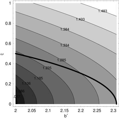
Figure 1: Surface plot showing values of $X_{+}$, the local minimum of $V(X^{2})$, as a function of $\omega$ and $b^{\prime}$. The bands denote degenerate values in decrements of $0.05$ starting at the top from $1.483$. The solid line represents eq. 14.

In fig. 2 we show a sample of numerical solutions for $X(r)$ for choices of $\omega,~{}b^{\prime}$, and $d$, which are well-approximated by the large $Q$-ball ansatz to be presented below. In fig. 3, we plot the numerically-evaluated $Q$-ball energy as a function of charge for different spatial dimensions. The left-hand side plot is for $b^{\prime}=2$ and the right hand side for $b^{\prime}=2.3$, covering the allowed range of values of $b^{\prime}$. The energy was obtained by first solving the equation for $\Phi(r)$ numerically (eq. 4, see fig. 2) and then using the result in eq. 13. There are several points to note: i) the existence of a minimum charge, $Q_{\rm min}$, below which $E/Q>1$; ii) the existence of $Q$-balls in higher dimensions and with considerably larger values of the charge $Q$; iii) the existence of a cusp in the region $E/Q>1$ for $d=3,~{}4,~{}5$ with a second branch, that is, the existence of different configurations with the same value of the charge. These are the $Q$-clouds described in ref. Q-clouds , which we were able to find for $d\leq 5$. We will come back to these three points below.

Figure 2: A sample of $Q$-ball profiles obtained numerically for various choices of $(\omega,~{}b^{\prime},~{}d)$. From left to right $(0.8,2.0,5),(0.6,2.0,3),(0.8,2.0,8)$. The dotted lines are the equivalent profiles from the ansatz of eq. 17.

Figure 3: $E/Q$ as a function of charge $Q$ for various dimensions. $b^{\prime}=2$ on the left and $b^{\prime}=2.3$ on the right.

Choosing a variational profile for the field has a degree of arbitrariness. Our guiding principle was a compromise between accuracy and calculability. Unfortunately, there is a sort of uncertainty principle operating here, in that higher accuracy implies in lower calculability and vice-versa. The works of refs. Woods used a Woods-Saxon ansatz for $d=3$. We verified that this ansatz is also quite accurate for $d\geq 3$ (matching closely the numerical solutions) but not as useful for the kind of analytical calculations we are interested in. We thus opted for the following simple ansatz for the field profile:

$$X(r)=\left\{\begin{array}[]{ll}X_{c}&\mbox{ if $r<R$}\\ X_{c}\exp[-\alpha(r-R)]&\mbox{ if $r\geq R$},\end{array}\right.$$ (17)

where $\alpha$ is a variational parameter to be determined.

Applying this ansatz to eq. 13 one obtains, after some algebra,

$$E[X] \leq \frac{c_{d}}{d}\left[\frac{1}{2}\omega^{2}X_{c}^{2}+V(X_{c}^{2})\right]R^{d}$$ (18)

$$+c_{d}(d-1)!\sum_{k=0}^{d-1}\frac{1}{k!}\left[\frac{A}{(2\alpha)^{(d-k)}}-\frac{B}{(4\alpha)^{(d-k)}}+\frac{C}{(6\alpha)^{(d-k)}}\right]R^{k}~{},$$

where,

$$A\equiv\frac{X_{c}^{2}}{2}(\omega^{2}+\alpha^{2}+1);~{}~{}B\equiv\frac{b^{\prime}}{4}X_{c}^{4};~{}~{}C\equiv\frac{X_{c}^{6}}{6}~{}$$ (19)

and we have used that $\int d^{d}x\rightarrow c_{d}\int r^{(d-1)}dr$. $c_{d}$ is related to the volume of the $d$-dimensional sphere, $v_{d}=c_{d}r^{d}$, with $c_{d}\equiv 2\pi^{(d/2)}/\Gamma(d/2)$. Using the ansatz, one can also obtain the conserved charge $Q$,

$$Q=\omega c_{d}X_{c}^{2}\left[\frac{R^{d}}{d}+(d-1)!\sum_{k=0}^{(d-1)}\frac{r^{k}}{k!(2\alpha)^{(d-k)}}\right]~{}.$$ (20)

A quick glance at the expressions for the energy and conserved charge and we can see that to proceed we must make simplifications. We will include only the dominant term from the surface contribution, proportional to $R^{(d-1)}$. As we will see, this approximation is quite accurate for large $Q$-balls. Using the expression for $Q$ in eq. 18 we obtain,

$$E_{Q}\leq\beta_{Q}^{2}R^{-d}+\frac{c_{d}}{d}V(X_{c}^{2})R^{d}+Zc_{d}R^{(d-1)}~{},$$ (21)

where we introduced the notation

$$\beta_{Q}^{2}\equiv\frac{dQ^{2}}{2c_{d}X_{c}^{2}}~{}~{};Z\equiv\frac{1}{2\alpha}\left[(1+\alpha^{2})\frac{X_{c}^{2}}{2}-\frac{B}{2}+\frac{C}{3}\right]~{}.$$ (22)

Before we extremise eq. 21 with respect to $R$, we extend Coleman’s result to $d$ dimensions, that is, we extremise the energy neglecting the surface term to obtain the zeroth-order approximation for the $Q$-ball radius,

$$R_{0}^{2d}=\frac{d\beta_{Q}^{2}}{c_{d}V(X_{c}^{2})}~{}.$$ (23)

Substituting $R_{0}$ into the expression for the energy (without surface term) we reproduce, as we should, Coleman’s result, $E_{R_{0}}[X_{c}^{2}]=\sqrt{2V(X_{c}^{2})/X_{c}^{2}}Q$: within this approximation, $Q$-balls exist if $\sqrt{2V(X_{c}^{2})/X_{c}^{2}}\leq 1$. Note that this approximation provides no information on the role of spatial dimensionality on the stability of $Q$-balls.

Imposing that $\partial E/\partial R|R_{c}=0$ into eq. 21 leads to the polynomial equation

$$c_{d}Z(d-1)R_{c}^{(2d-1)}+c_{d}V(X_{c}^{2})R_{c}^{(2d)}-d\beta_{Q}^{2}=0~{}.$$ (24)

In order to find an approximate solution, valid for large $Q$-balls, we write the critical radius as $R_{c}\simeq R_{0}+\delta R$, where $\delta R\ll R_{0}$. Substitution into the above equation leads to an expression for $\delta R$ and thus for $R_{c}$,

$$\delta R=-\frac{(d-1)Z}{2dV(X_{c}^{2})}~{}.$$ (25)

We now substitute this approximate expression for $R_{c}$ into the expression for the energy, eq. 21, to obtain,

$$E_{Q}[X_{c}]|_{R_{c}}=\sqrt{2V(X_{c}^{2})/X_{c}^{2}}Q\left[1+\xi Q^{-1/d}\right]~{},$$ (26)

where we introduced

$$\xi\equiv\frac{dZ}{2}\left(\frac{c_{d}}{d}\right)^{1/d}\left[\frac{X_{c}^{2}}{\left[V(X_{c}^{2})\right]^{(2d-1)}}\right]^{(1/2d)}~{}.$$ (27)

This expression for the energy depends still on the variational parameters $X_{c}$ and, through the expression for $Z$ (cf. eq. 22), on $\alpha$. Ideally, one would extremise it for these two variables to obtain a final expression for the energy given only in terms of the spatial dimensionality $d$ and the asymmetry parameter $b^{\prime}$. Although this task cannot be done exactly, it can be done approximately. The final test for the efficacy of the approximations will be to compare the analytical expression of the energy to its numerical evaluation shown in fig. 3. An estimate for $X_{c}$ can be obtained by extremizing the energy neglecting the surface term, that is, by extremizing Coleman’s expression $E_{R_{0}}[X_{c}^{2}]=\sqrt{2V(X_{c}^{2})/X_{c}^{2}}Q$. One obtains,

$${\bar{X}}_{c}^{2}=\frac{3}{4}b^{\prime}~{}.$$ (28)

Although, to quote Coleman Coleman , neglecting the surface term amounts to a “brutal set of approximations,” this analytical result for the core value of the field proves to be quite reasonable. This is due to the fact that $X_{c}$ is only mildly dependent on $d$ and $b^{\prime}$.

In order to extremise $\alpha$ we revert to the expression for the energy in eq. 21, and note that $\partial E/\partial\alpha=\partial Z/\partial\alpha$, where $Z$ is defined in eq. 22. One can easily obtain that

$$\alpha_{c}^{2}=1-\frac{b^{\prime}}{4}X_{c}^{2}+\frac{X_{c}^{4}}{9}=1-\frac{b^{\prime 2}}{8}~{},$$ (29)

where in the last step we used eq. 28. Using these results in eq. 26, we obtain the promised extremised expression for the $Q$-ball energy in terms of $d$ and $b^{\prime}$,

$$\frac{E_{Q}[d,b^{\prime}]}{Q}\simeq\sqrt{1-\frac{3}{16}b^{\prime 2}}\left[1+\xi(d,b^{\prime})Q^{-1/d}\right]~{},$$ (30)

where,

$$\xi(d,b^{\prime})=\frac{3d}{16}\left(\frac{c_{d}}{d}\right)^{1/d}b^{\prime}\sqrt{1-\frac{b^{\prime 2}}{8}}\left[\frac{3b^{\prime}}{4\left[\frac{3b^{\prime}}{8}\left(1-\frac{3b^{\prime 2}}{16}\right)\right]^{2d-1}}\right]^{1/2d}~{}.$$ (31)

Glancing at eq. 30, we can see that since the contribution from the surface term is positive, the lower bound on the $Q$-ball energy is $E/Q>\sqrt{1-\frac{3}{16}b^{\prime 2}}$, which interestingly, is the same as saying $E/Q>\omega_{c}$ where $\omega_{c}$, defined in eq. 14, is the minimum value that gives a solution to eq. 4. Note that as $b^{\prime 2}\rightarrow 16/3$, which is the critical value for $V(\Phi=0)$ to be the global minimum, the term proportional to $Q^{-1/d}$ dominates the expression for $E/Q$, which is finite for all $b^{\prime}$.

In fig. 4 we contrast the numerical results (see fig. 3) with those obtained from the analytical approximation of eq. 30 for different values of $b^{\prime}$ and $d$ as a function of $Q$. For clarity, we introduced the percentual difference $\Delta\equiv\left(E/Q|_{\rm num}-E/Q|_{\rm anal}\right)/E/Q|_{\rm num}$. We plot $\Delta$ vs. $Q$, showing that there is a wide range of parameter space where the approximation is better than $20\%$. The agreement gets worse as $b^{\prime}$ and $d$ increase, although it always improves for larger values of $Q$ as one would expect from an approximation describing large $Q$ balls. We will soon offer a criterion to define what is a large or small $Q$-ball.

Figure 4: Contrasting the numerical and analytical expressions for the energy as a function of charge $Q$ for various dimensions and $b^{\prime}=2.0$. $\Delta\equiv\left(|E/Q|_{\rm num}-E/Q|_{\rm anal}|\right)/E/Q|_{\rm num}$. Note that, although not shown, the lines continue to decrease monotonically as $Q$ increases, and the approximation improves.

IV Small Q-Balls: Variational Approach

$Q$-balls can also be “small,” that is, not well-described by the widely adopted thin-wall approximation, consistent with the results above. Small $Q$-balls will have radii $R\gtrsim m^{-1}_{\phi}$. A sample of such configurations are shown in fig. 5.

Figure 5: Comparison between numerical solution and gaussian profile for a few sample “small” $Q$-balls. $b^{\prime}=2.3$ throughout. On the left $d=3$ and on the right $d=4$.The solid lines are the numerical solutions to eq. 4, while the dashed lines are the gaussian approximations of eq. 32. From left to right, $Q=33,45,225,519$.

In order to obtain analytical insight into these objects, we will adopt a gaussian ansatz for their profile,

$$X(r)=X_{c}\exp[-r^{2}/R^{2}]~{}.$$ (32)

This approach, in contrast to that of ref. Kusenko97 which used an approximate 3d bounce solution, is particularly simple to adopt in an arbitrary number of spatial dimensions. Using the gaussian profile above in the expression for the energy eq. 13 and using dimensionless variables, we obtain,

$$E_{Q}[X_{c},R]=\left(\frac{\pi}{2}\right)^{d/2}\left[\beta_{Q}^{2}R^{-d}+\alpha R^{(d-2)}+\gamma R^{d}\right]~{},$$ (33)

where we introduced,

$$\beta_{Q}^{2}=\left(\frac{2}{\pi}\right)^{d}\frac{Q^{2}}{X_{c}^{2}};~{}~{}\alpha=dX_{c}^{2};~{}~{}\gamma=\frac{X_{c}^{2}}{2}-\frac{b^{\prime}}{2^{d/2}}\frac{X_{c}^{4}}{4}+\frac{1}{3^{d/2}}\frac{X_{c}^{6}}{6}~{}.$$ (34)

The conserved charge is,

$$Q=\left(\frac{\pi}{2}\right)^{d/2}\omega X_{c}^{2}R^{d}~{}.$$ (35)

Note that with the gaussian ansatz, it is easy to obtain the energy for arbitrary polynomial potentials d-oscillons . Writing $V(\Phi)=\sum_{n=1}^{h}\frac{g_{n}}{n!}\Phi^{n}$, and $\Phi=A\exp[-r^{2}/R^{2}]+B$ ($B$ is the asymptotic vacuum), we get, $\int r^{(d-1)}V(\Phi)dr=\frac{\Gamma(d/2)}{2}R^{d}\sum_{n=1}^{h}\frac{A^{n}}{n^{d/2}n!}\frac{d^{n}V}{d\Phi^{n}}|_{B}$.

By extremizing the expression for the energy, and adopting the same approximation as in the previous section ($R_{c}=R_{0}+\delta R$), one computes the critical radius,

$$R_{c}=R_{0}\left[1-\frac{(d-2)}{dR_{0}^{2}}\frac{\alpha}{\gamma}\right]~{},$$ (36)

where $R_{0}$ is the zeroth-order result, obtained by neglecting the surface term (proportional to $\alpha$ in eq. 33, exact for $d=2$),

$$R_{0}^{2d}=\frac{\beta_{Q}^{2}}{\gamma}~{}.$$ (37)

Including the surface term decreases the radius as it should. The next step is to substitute this critical radius back into the expression for the energy, eq. 33. We found it useful to write $R_{c}=R_{0}(1-\varepsilon)$ to keep track of the radial corrections induced by the surface term (proportional to $\alpha$). The final result is

$$E_{Q}[X_{c}]=\frac{\gamma^{1/2}}{X_{c}}Q\left[2+\xi Q^{-2/d}-\frac{(d-2)^{2}}{d}\xi^{2}Q^{-4/d}\right]~{},$$ (38)

where,

$$\xi=\frac{\pi}{2}\frac{\alpha}{\gamma^{(d-1)/d}}X_{c}^{2/d}~{}.$$ (39)

This way of expressing the result makes it clear what the zeroth-order value for the energy is ($\xi=0$) and the role of surface corrections in arbitrary dimensions. It is also quite useful to test the validity of the gaussian approximation in the computation of the critical charge $Q_{\rm min}$, below which $E/Q>1$, (see fig. 3). We use the value of $X_{c}$ in terms of $b^{\prime}$ given by eq. 28, since it proves to be quite accurate (cf. figs. 1 and 5). Thus, $\alpha$, $\gamma$, and $\beta_{Q}^{2}$ can be expressed in terms of $d$, $b^{\prime}$, and $Q$ as in the previous section.

In fig. 6 we contrast the analytical and numerical values for the $Q$-ball energy as a function of $Q$ for $b^{\prime}=2$ (left) and $b^{\prime}=2.3$ (right) for $d=3,~{}4,~{}5$, and $6$. As for the large-charge regime, there is a wide window of parameter space well-described by the gaussian approximation. As the charge increases the agreement gets worse. This is easily understood by examining the “friction” term in the equation for $\Phi(r)$, eq. 4. As $Q$ increases the particle spends more “time” not moving ($\Phi^{\prime}\simeq 0$, the motion is initially friction-dominated) until $r$ grows large enough and the term becomes subdominant. Since a gaussian profile does not approximate well a flat core, the approximation gets worse for large $Q$ configurations. As before, we use $\Delta\equiv\left(E/Q|_{\rm num}-E/Q|_{\rm anal}\right)/E/Q|_{\rm num}$.

Figure 6: Contrasting numerical and analytical estimates for the $Q$-ball energy for $d=3$, $4$, $5$, and $6$ (from left to right). $b^{\prime}=2.0(2.3)$ on the left(right). It is clear that the gaussian ansatz provides a good approximation for $Q$-balls with relatively low charge.

We can now put the results of our analytical approximations together, comparing their respective range of validity. In fig. 7 we plot the percentual errors ($\Delta$) for both approximations and $b^{\prime}=2$. [As $b^{\prime}\rightarrow 2.3$ one should use the gaussian approximation as long as $Q$ is small enough, as can be seen in fig. 6.] Note how the lines cross at a given charge $Q_{c}$ for each value of $d$. Clearly, one is to use the approximation with the smallest error: configurations with $Q\leq Q_{c}$ are best approximated by the gaussian ansatz: they can be called “small” $Q$-balls. Configurations with $Q>Q_{c}$ are better described by the exponential ansatz of the previous section; they can be called “large” $Q$-balls. Choosing one or the other approximation, we are able to keep the errors quite small for different values of $d$. For example, for $d=4$ and $b^{\prime}\gtrsim 2$, the error can be kept below $15\%$. This illustrates the validity of our analytical approximations and their power to express the properties of $Q$-balls in an arbitrary number of dimensions.

Figure 7: Contrasting the absolute errors of the variational estimates for the energy of $Q$-balls for several values of spatial dimensionality $d$. All plots are of $b^{\prime}=2.0$. The positive slope line is for the gaussian approximation while the negative slope line is for the exponential-decay approximation of the previous section.

As a final result, we can use the gaussian ansatz to obtain an approximate expression for the lowest value for the $Q$-ball charge, $Q_{\rm min}$. Imposing $E/Q=1$ on eq. 38, one obtains a polynomial identity, which is solved for

$$Q_{\rm min}^{2/d}=\frac{\xi}{2c}\left[1-\sqrt{1-\frac{4(d-2)^{2}c}{d}}\right]~{},$$ (40)

where $c\equiv X_{c}/\sqrt{\gamma}-2$. Note that for $d=2$ there is no restriction on the minimum charge. That is not the case in higher dimensions. We can use $X_{c}^{2}=3b^{\prime}/4$ to obtain an expression of $Q_{\rm min}$ in terms $b^{\prime}$ and $d$. In fig. 8 we show $Q_{\rm min}$ as a function of $d$ for $b^{\prime}=2.0$ (circles) and $b^{\prime}=2.3$ (squares). Filled symbols were computed using the gaussian ansatz above, while open symbols were obtained numerically (cf. fig. 3). The continuous lines are exponential fits $Q_{\rm min}\sim\exp[d]$. $Q$-balls, even those with minimal charge, grow quite large in higher dimensions, not a surprising result given that the charge is given by a volume integral. As $d$ increases, the gaussian prediction for the minimum charge becomes worse for reasons explained above.

Figure 8: Minimum stable $Q$-ball charge vs. spatial dimensionality. The circles (squares) represent $b^{\prime}=2.0,(2.3)$ The filled dots are the results from the gaussian approximation, eq. 40. The dashed (solid) lines are exponential fits to the numerical values.

V $d$-Dimensional $Q$-Clouds

Q-clouds are classically unstable solutions ($E/Q>1$) that exist as $\omega\rightarrow 1$ found for $d=3$ in ref. Q-clouds . They belong to the upper branch of fig. 3, starting at $Q_{\rm min}$, characterized by low core field values and large radii. Two examples can be seen in fig. 9.

It is quite simple to understand the qualitative nature of these solutions. Recall, from eq. 4, that the solution traces the motion of a “particle” in the potential $-U(\Phi)$, with a quadratic term, $\frac{1}{2}(1-\omega^{2})\Phi^{2}$, and a friction term $\frac{d-1}{r}\Phi^{\prime}$. The boundary condition at spatial infinity is, as for $Q$-balls, $\Phi\rightarrow 0$. As $\omega\rightarrow 1$, the hill at $U(0)$ gets shallower. Thus, it becomes easier for the particle to reach $\Phi=0$. As a consequence, the value of the field at $r=0$, $\Phi_{c}$, must decrease to avoid overshooting. The correct solution is obtained when $\Phi_{c}$ is just large enough for the “particle” to overcome the friction and come to rest at $-U(\Phi=0)=0$ as $r\rightarrow\infty$.

The transition from a $Q$-ball to a $Q$-cloud is controlled by the value of $\omega$. Alford has shown that there is a critical value of $\omega$, $\omega_{\rm min}$, above which the unstable $Q$-ball becomes a $Q$-cloud Q-clouds . We have found that, indeed, the same behavior persists for $d=4$ and, marginally, for $d=5$. for $d=6$ we found that $\omega_{\rm min}\rightarrow 1$, as shown in fig. 10. Clearly, as $d$ increases, and thus the “friction,” $\Phi_{c}$ must also increase. We illustrate this in fig. 9 where, for the same parameters ($b^{\prime}$ and $\omega$), $\Phi_{c}$ grows substantially with $d$. Numerically, we were unable to find $Q$-clouds for $d\geq 6$. Apparently, in higher dimensions only $Q$-balls, with larger values of $\Phi_{c}$ to overcome the hill at $-U(0)$, are possible. Although we have not proven this, we have determined that $Q$-clouds are only possible if $\Phi_{c}<\Phi_{\rm inf}$, where $\Phi_{\rm inf}$ is the inflection point nearest to the origin.

Figure 9: Q-cloud profiles for $d=4,3$ (upper,lower) for identical parameters $b^{\prime}=2.0,\omega=0.99999$.

Figure 10: Q vs. $\omega$ for spatially-bound configurations in different spatial dimensions and $b^{\prime}=2$. Those with $\omega\leq\omega_{min}$ are $Q$-balls, while those with $\omega>\omega_{min}$ are $Q$-clouds. Note that $\omega_{min}\rightarrow 1$ for $d\geq 6$.

VI Concluding Remarks

We have presented a detailed study of $Q$-balls in an arbitrary number of spatial dimensions for potentials of the form $V(\phi\phi^{\dagger})=\sum_{n=1}^{3}a_{n}(\phi\phi^{\dagger})^{n}$, where $a_{n}$ is a constant. Numerical solutions were obtained and contrasted with simple analytical ansatze, separated into “large” and “small” $Q$-balls. It was shown that it is possible, for most of the parameter space, to use the analytical expressions with comfortable accuracy to compute the $Q$-balls’ energy and radii as a function of only the spatial dimensionality and a single parameter defining the potential energy density of the model. We have also obtained approximate analytical expressions for the minimum charge for $Q$-balls to be stable, $Q_{\rm min}$, showing in addition how it depends on spatial dimensionality. An empirical relation was found for the dependence of the minimum charge on spatial dimensionality, $Q_{\rm min}\sim\exp[d]$. Finally, we also explored the properties of $Q$-clouds in $d$ dimensions for the same type of potentials. We provided qualitative arguments as to why we were unable to find such solutions for $d\geq 6$.

$Q$-balls have been studied with great interest since Coleman introduced them in 1985. We hope that the present work will be useful to establish their possible role in models that make use of extra spatial dimensions. By exploring the properties of spatially-bound nonlinear objects in an arbitrary number of dimensions we gain insight not only on the nature of such objects from a general viewpoint, but also on the role of dimensionality on the properties of nonperturbative configurations. Such objects, if existent, will no doubt have an impact on the physics of the vacuum and of the early universe, and may well influence the dynamics of spatial compactification.

MG was supported in part by a National Science foundation Grant no. PHYS-0099543.

References

- (1) Solitons: Introduction and Applications, ed. M. Lakshmanan (Springer-Verlag, Berlin, 1988).
- (2) R. Rajamaran, Solitons and Instantons (North-Holland, Amsterdam, 1987).
- (3) C. G. Callan, J. Harvey, and A. Strominger, Nucl. Phys. B 367 (1991) 60; ibid. B 359 (1991) 611; for a more recent example, A. L. Larsen and A. Khan, Nucl. Phys. B 686 (2004) 75.
- (4) Modern Kaluza-Klein Theories, ed. T. Appelquist, A. Chodos, and P. G. O. Freund, (Addison-Wesley, Menlo Park, CA 1987); An Introduction to Kaluza-Klein Theories, ed. H. C. Lee, (World Scientific, Singapore 1984).
- (5) L. Randall and R. Sundrum, Phys. Rev. Lett. 83 (1999) 3370; ibid. 83 (1999) 4690.
- (6) N. Arkani-Hamed, S. Dimopoulos, G. Dvali, and N. Kaloper, Phys. Lett. B 429, 263 (1998); Phys. Rev. Lett. 84, 586 (2000); for a review see, I. Antoniadis, Nucl. Phys. B (Proc. Suppl.) 127, 8 (2004).
- (7) C. Csaki, TASI Lectures on Extra Dimensions, hep-ph/0404096.
- (8) V. A. Rubakov, Large and Infinite Extra Dimensions, Phys.Usp. 44 (2001) 871-893; Usp.Fiz.Nauk 171 (2001) 913-938. [arXiv:hep-ph/0104152]
- (9) G. F. Giudice, R. Rattazzi, and J. D. Wells, Nucl. Phys. B 544 (1999) 3.
- (10) I. Antoniadis, K. Benakliand, and M. Quirós, Phys. Lett. B 460 (1999) 176.
- (11) M. Gleiser, Phys. Lett. B 600, 126 (2004).
- (12) S. Coleman, Nucl. Phys. B 262, 263 (1985).
- (13) G. H. Derrick, J. Math. Phys. 5, 1252 (1964).
- (14) T. D. Lee and Y. Pang, Phys. Rep. 221, 251 (1992).
- (15) A. Safian, S. Coleman, and M. Axenides, Nucl. Phys. B 304, 403 (1988).
- (16) K. Lee, J. A. Stein-Schabes, R. Watkins, and L. M. Widrow, Phys. Rev. D 39, 1665 (1989); K. N. Anagnostopoulos, M. Axenides, E. Floratos, and N. Tetradis, Phys. Rev. D 64, 125006 (2001); T. Levi and M. Gleiser, Phys. Rev. D 66, 087701 (2002).
- (17) A. Kusenko, Phys. Lett. B 405, 108 (1997); M. Axenides, E. Floratos, and A. Kehagias, Phys. Lett. B 444, 190 (1998).
- (18) M. Axenides, S. Komineas, L. Perivolaropoulos, Phys. Rev. D 61, 085006 (2000); R. A. Battye and P. M. Sutcliffe, Nucl. Phys. B 590, 329 (2000).
- (19) N. Graham, Phys. Lett. B 513, 112 (2001).
- (20) J. Frieman, G. Gelmini, M. Gleiser and E. W. Kolb, Phys. Rev. Lett. 60, 2101 (1988); J. A. Frieman, A. V. Olinto, M. Gleiser, and C. Alcock, Phys. Rev. D 40, 3241 (1989); A. Kusenko and M. Shaposhnikov, Phys. Lett. B 418, 46 (1998).
- (21) M. Alford, Nucl. Phys. B 298, 323 (1988).
- (22) S. Coleman, Phys. Rev. D 15, 2929 (1977).
- (23) A. Kusenko, Phys. Lett. b 404, 285 (1997).
- (24) R. Friedberg, T. d. Lee, and A. Sirlin, Phys. Rev. D 13, 2739 (1976).
- (25) T. A. Ioannidou and N. D. Vlachos, J. Math. Phys. 44, 3562 (2003); T. A. Ioannidou, V. B. Kopeliovich, and N. D. Vlachos, Nucl. Phys. B 660, 156 (2003); T. A. Ioannidou, A. Kouiroukidis, and N. D. Vlachos, J. Math. Phys. 46, 042306 (2005).