A statistical formalism of Causal Dynamical Triangulations
Abstract
We rewrite the 1+1 Causal Dynamical Triangulations model as a spin system and thus provide a new method of solution of the model.
1 Introduction
The failure of perturbative approaches to quantum gravity has motivated theorists to study non-perturbative quantization of gravity. These seek a consistent quantum dynamics on the set of all Lorentzian spacetime geometries.
One such approach which has led to very interesting results is the causal dynamical triangulation (CDT) approach[1, 2]. In the interest of understanding why this approach leads to non-trivial results, in this paper we study a reformulation of it as a spin system. The basic idea is that causal structure is coded into the values of a set of spins, in such a way that causal relations are expressed as constraints on the allowed spin configurations. This makes possible a new method of studying the model which is complementary to that used in the original papers. In this paper we study only the dimensional model[1], but we believe the method described here generalizes to higher dimensions and can include matter.
In the next section, we review the CDT model in dimensions and the solution to it given by Ambjorn and Loll in [1]. In section 3, we reformulate the CDT model as a spin system, which we call the statistical model. In section 4, we show how to solve the model by a procedure made natural by the translation of the model into a spin system. In section 5, we discuss the application to the model of the renormalization group, after which we close with a brief discussion of what we learned about quantum Lorentzian geometry from the translation to a spin system.
2 Definition of the model
In this section, we review Causal Dynamical Triangulations, as defined in [1].
Causal Dynamical Triangulations is arrived at by a discretization of the path integral for quantum general relativity in dimensions. In 1+1 dimensions, the continuum Einstein action is
| (1) |
where , and . is the element of area and is the cosmological constant. The metric represents the geometry of spacetime.
We define the amplitude to evolve from an initial geometry, which is a circle of length , to a final geometry, a circle of length , formally by
| (2) |
where the sum is over geometries with fixed topology , is the measure and the boundaries of the histories are two circles of lengths and .
We now discretize this path integral. A given history is represented by a set of spacelike circles (or rings), which are labelled . These are considered time slices in some fixed gauge [6]. Each ring has vertices, connected by edges which are assumed to be of length unity in Planck units. It is required that every time-slice has at least one edge.
The vertices of two adjacent loops are connected by a set of timelike edges of length-squared . These define the causal structure of the discrete history and are chosen so that the surface is broken up into triangles. To ensure this, the leftmost future vertex of a vertex -th of is the rightmost future vertex of the vertex -th of the same ring. A triangle has one spacelike edge, which sits on one of the spacelike edges of and two timelike edges, which connect two vertices of to either one vertex of ( “up” triangle), or two vertices of (“down” triangle). Each history is then a piecewise flat Lorentzian geometry. In each triangle , and the action becomes , where is the summation of the areas of triangles. The area of each Lorentzian triangle is [5]. Therefore, the action of a time-slice consisting of triangles is . We absorb the factor of in and the action becomes .
The path integral amplitude for the propagation from geometry and is the sum
| (3) |
over all such piecewise flat manifolds defined in this way with initial and final circles fixed. Note that the cosmological constant is replaced by the “bare” cosmological constant . Note also that topology change is excluded by the requirement that each history have topology .
In summary, the following are key assumptions of the model:
-
1.
Fixed topology: the topology of the boundaries and interpolating spacelike slices is and each history is . Each slice has length .
-
2.
The amplitudes are given by a path integral: the amplitude of propagation from the initial ring to the final ring is given by the sum over all interpolating histories.
-
3.
Histories are triangulations: the leftmost future vertex of a vertex -th of is the rightmost future vertex of vertex -th of .
2.1 Review of the generating function method
In this subsection we review briefly the method of solution of the problem given in [1].
Let there be vertices in and vertices in . If vertices of are in the future of the vertex of then, because of condition 3, the total number of vertices of is . The two spatial rings are connected by triangles; of which are “up” and are “down”.
To propagate from to in one time-slice, the action is and the amplitude is
| (4) |
Generally, if we mark the vertices of the initial ring, the amplitude becomes
| (5) |
where the denotes that the vertices of the initial ring are marked. If we mark the vertices of the final loop, the amplitude becomes
| (6) |
Using the conditions 2 and 3, the corresponding amplitude between times and can be written as:
| (7) |
With marked initial vertices, the amplitude is:
| (8) |
Thus, we are able to write the amplitude of evolution from to with initial vertices and final vertices as:
| (9) |
To solve equation (9), we Laplace transform it,
| (10) |
with the definitions , and in which and are the cosmological constant on the initial and final boundaries respectively. Using the Laplace transformation (10) on equation (9), we obtain the one-time-step :
| (11) |
The amplitude in terms of defines the region of convergence , and . The iterative relation on the Laplace transformed amplitude is then
| (12) |
Ambjorn and Loll in [1] showed that the iterative relation can be written in a simpler way:
| (13) |
The corresponding equations for the Laplace transformed amplitudes are:
| (14) |
| (15) |
The asymmetry between and in the expression (11) is due to the marking of the initial ring. If we also had marked the final ring, the corresponding generating function would be obtained from by acting with (which is equivalent of multiplying by ):
| (16) |
The corresponding generating function is obtained from
by acting with ,
| (17) |
In the continuum limit we expect that the bare propagators are subject to a wave-function renormalization. However, all coupling constants with positive mass dimension undergo an additive renormalization, while the partition function undergoes a multiplicative wave-function renormalization [4]. The only non-trivial continuum limit of eq. (13) is obtained when , so for . The singular Green’s function can be cured by multiplying it by a cut-off dependent factor [4]. This limit is equivalent to . Thus, from the convergence condition, we find (at .
3 The dual statistical model
We now recast the 1+1-dimensional Causal Dynamical Triangulations model as a spin system with certain constraints on their configurations and couplings, reflecting the geometric properties of the CDT.111Another statistical mechanical approach to the cdt model is developed in [3]”
We proceed as follows. Each triangle will be regarded as a spin . We associate to each down triangle (with two vertices on and one on ) an up spin and to each up triangle (with two vertex on and one on ) a down spin. Spins can take two possible values, when they come from an up triangle, and when they correspond to a down triangle. The spins will live on a trivalent lattice and we find it convenient to graphically denote the two states of a spin as:
| (18) |
The dashed line represents the triangle dual to each spin. Each spin has one black head and two white head, which are dual to one spacelike edge and two timelike edges, respectively.
Gluing two triangles along a common edge defines a spin-spin interaction. The CDT weighing of the triangulations means there are two kinds of interactions: gluing two triangles along their spacelike edges gives a spin-spin interaction of strength , while a gluing of two timelike edges corresponds to coupling as follows:
| (19) |
No gluing of a timelike to a spacelike edge is allowed. We have incorporated these couplings to the graphical notation (18): the interaction between two black heads of two spins occurs with the spin-spin interaction coupling , and the interaction between two white heads does with a coupling.222Sometimes in this paper we call coupling the “white interaction” because of the coupling it provides between two white heads, and coupling the “black interaction” because of the coupling it provides between two black heads.
In an ordinary spin system, the values of spins are not related to the structure of the lattice. The lattice is fixed while the values of the spins on the nodes vary. However, in a model of gravity we do not have any pre-assigned lattice, since the spacetime is completely dynamical. In our formalism spacetime is created by the configurations of the spins.
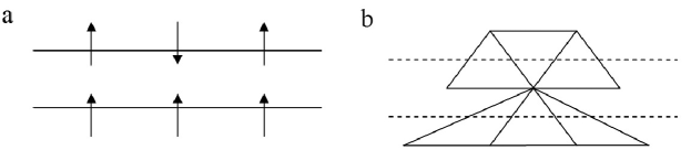
Let us look at a simple example to explain how the spins relate to the causal structure and geometry. In Figure 1(a), we see a lattice consisting of two rows with a certain number of spins. In an ordinary spin system without an external field, the spins fluctuate independently of the lattice. However, in our model, the spins define the causal structure of the resulting geometry. Following the rules just described, Figure 1(a) is interpreted as a dual geometry, shown in Fig. 1(b). We see from Figure 1(b) that the spins in Fig. 1(a) define a geometry that does not satisfy the causality constraints of CDT. The dual spacetime is not causal as there are vertices in the second slice that have no past in the initial slice.
We will impose constraints on the dual spin system so that all spin configurations have dual CDT histories:
-
1.
Causality constraint: Each up spin in row () must be coupled to a down spin in row , with coupling .
-
2.
Non-degeneracy constraint: Every row has at least one spin.
A spin system that satisfies these constraints is dual to a history of the CDT model. 333From the point of view of statistical physics, the present model is analogous to a“diluted” 2 dimensional classical Ising model because the number of spins in each time-slice can vary (see, for example, [7]).
It is instructive to give an example of a spin configuration that does satisfy the causality constraints. The triangulation
![[Uncaptioned image]](/html/hep-th/0505165/assets/x4.png) |
(20) |
in the dual spin system is:
![[Uncaptioned image]](/html/hep-th/0505165/assets/x5.png) |
(21) |
The amplitude of this history is:
| (22) |
Note that the dual spin system can be read as a history somewhat analogous to a Feynman diagram. The history of (21) begins with three initial black circles, and ends with two final black circles. In between there are two moments of discrete time, given by the rows of couplings. There are no unpaired black or white circles, except for the initial and final black ones (recall that we have cylindrical boundary conditions on the boundary white ones).444An example of the spacetime structure with equal intermediate rings can be thought of as the tower of Pizza (from above of which Galilei did his famous gravitational experiment).
Next, we use this definition of the model to count the 2d CDT histories.
4 Computing CDT amplitudes using the dual spin system
We now want to calculate the 1+1 CDT path integral amplitude from a given initial ring to a given final ring, using the dual spin system. Here, the evolution amplitude is given by a correlation function between the spins of the boundary rows.
We will find it convenient to introduce a notion of effective spins, which allows us to sum the causal histories.
4.1 Single-row configurations
We will illustrate the spin system solution by first calculating the CDT amplitude for a single row of spins. This means all spin configurations on rows containing from one to infinite number of spins, subject to the causality and non-degeneracy constraints.
In fact, for one row, we only have the non-degeneracy constraint, which we impose using what we call “the box”. A box is two spins with opposite orientations, with one coupling. This is denoted by
| (23) |
The superindex (1) is a reminder that we are working with one-row configurations. The geometric constraint is equivalent to requiring that each row must contain at least one box.
For a single row of spins, there are no couplings and we have simply the combinatorics of spins attached to a box. In a row of spins, two of them have to make a box, and are no longer free to be up or down555Since the spins are located on a closed chain, the amplitude is not sensitive to locations of spins. On the other hand since the free black heads on the initial and final rings are marked, different location of among spins is counted as a different configurations., hence,
| (24) |
where is the number of ways of choosing two consecutive marked spins (the box) among spins, .
For example, for :
| (25) |
This amplitude is actually the Laplace transformed amplitude, similar to a Greens function. In the dual triangulation, the Laplace inverse transform of the above is the amplitude to go from an initial ring of length to a final ring of length . So we have to add up all Laplace transformed amplitudes for different ring lengths (spin number and configurations) to derive the Green’s function.
The single-slice amplitude, , is
| (26) |
To perform the sum, we redefine to obtain:
| (27) | |||||
We now define the quantity , so that the above equation can be rewritten as
| (28) |
For , eq. (28) sums to the same result of (16):
| (29) |
4.1.1 Non-marked vertex amplitude
Comparing the amplitude (29) with the results of [1], we see our result is symmetric on and since both our up and down spins are marked. To derive the exact result of Ambjorn and Loll in [1] we need unmarked up spins.
We can illustrate this for :
| (30) |
Since the top black circles are not distinguished, we have only one term with 3 up spins. For two up spins there are three terms, for the possible permutations of the two marked down spins, etc.
Summing over all spins, we find the unmarked amplitude for one row to be:
| (32) | |||||
| (33) |
To sum the infinite series we use a simple trick. We add and subtract from the amplitude (33) to find
| (34) | |||||
which is the same result of the unmarked one-step transfer matrix amplitude (11). It is easy to see that using the eq. (15),
| (35) |
In fact (the corresponding amplitude of marked initial and final spins in slices) is exactly equivalent to the solution of the generating function method.
4.2 Two-row configurations: the effective spin
Our solution of the CDT departs from the transfer matrix method of [1] when more than one row is considered. For a spin configuration of rows of spins, we will introduce an effective spin which makes the rows of spins a single row of these effective spins. Once the appropriate form of the effective spin has been found the remaining calculation is very straightforward. 666Let us remind that any horizontal sequence of black heads make a time-slice as well as any horizontal sequence of white heads.
The form of the effective spin is different for odd or even . We start with the 2-row effective spin . This effective spin has the form
| (36) |
where the gray spins denote rows with spins from zero to infinity so that the above diagram is
| (37) | |||||
| (38) |
Note that the solid black part of is the implementation of the causality constraint for two rows.
To calculate the two-row amplitude , we first need . The diagram of differs from in that in the number of the gray spins run from zero to infinity while in they run from one to infinity. In other words, the presence of at least one up spin in the final row and one down spin in the initial row is guaranteed. However, the end row spins are distinguishable and have to be counted separately. We thus easily find the amplitude for to be:
| (39) |
The amplitude is obtained from all possible configurations of effective spins attached to one . Since the spins are marked, as in the amplitude of the one-row case, the position of has to be taken into account. The final result is:
| (40) |
4.3 The odd and even effective spins
We can now generalize the method we used to count one- and two-row Green’s functions to the general case. We shall find it useful to consider separately the cases of even and odd numbers of slices. Since there is no interaction between a white and a black head, we can divide interactions and cover all black interactions by defining the notion of effective spin, and white-interact them along their common time-slice (-slices).
Note that, in the one-row case, there were two values of spin , up and down. In the two-row case, there is only one type of effective spin. This generalizes: even-row configurations can be mapped to single-row with one type of effective spin, while odd-row configurations need two-valued effective spins.
4.3.1 Odd effective spins
It is instructive to find the effective spin for three rows first. One can see that all three-row configurations can be constructed from these two building blocks:
| (41) |
The labels 0, 1, 2 and 3 on the black heads denote the order of the rows, from initial, 0, to final, 3. There are two different sequences of spins in each one of the effective spins. has a sequence of spins in row 3, while has a sequence of spins in row 1. Again, the number of gray spins varies from one to infinity.
and can white-interact by their common white heads. In fact, any the connection between the initial slice (the zeroth row) and the final slice (the 3rd row) occurs if and only if at lease one white-interacts with at least one . This minimal interaction makes .
We evaluate as previously. We need at least one and one in each configuration. The initial and final loops all spins are marked and thus it matters which one of the gray spins we convert to a black spin (whose presence is necessary in ). Thus, like (23) we have:
| (42) | |||||
The three-row amplitude is now easily derived from the possible configurations of effective spins on a single :
| (43) |
Generalizing this, it is straightforward to check that, for odd-row configurations, , and amplitude are:
| (44) |
| (45) |
| (46) |
where .
4.3.2 Even effective spins
To find a generalized formula for even rows, it is useful to study first the case of four rows.
The easiest way to calculate the corresponding effective spin in four rows is by comparing it with the two rows. We take the two components of as the new fundamental spins so that has the same form as (36), but with the replacing the :
| (47) |
We can now calculate . Diagrammatically, it is
Each box represents a spin and the number of boxes ranges from zero to infinite. In the diagram, we should guarantee the existence of at least two “I” shapes for the two intermediate slices. One of them is located inside one of the bottom row of boxes and the other one inside one of the top ones. In the above diagram they were indicated in black color. In addition to these two “I” shapes, we must also guarantee the existence of at least one (i.e. ) in the initial time-slice and one (i.e. ) in the final time-slice, in order to connect initial and final rings with the least number of connections between slices. How can we choose the and spins? A suggestion is that they are chosen among the other gray spins inside the boxes. Although, the suggestion is problematic because, in general, the two spins may appear inside two boxes that are different than the previously guaranteed ones. Therefore the existence of such boxes, which support the two spins, should be guaranteed first. The existence of the box requires the existence of its “I” shape part. Turning on more gray “I” shapes, does not meet the initial motivation of defining the notion of , which was any necessary connection between the initial and final rings such that at every ring the existence of only one spin is guaranteed (due to non-degeneracy constraint).
Another suggestion for supporting the existence of these two spins is that some spins live independently (with respect to boxes) on the initial and final rings and among them the existence of one up and one down ones is guaranteed. The idea is acceptable since it meets the condition of the least number of guaranteed spins among the most arbitrary configuration of connections between the initial and final rings (which is 6 in this case).
Therefore the weight of can be generally written:
| (48) | |||||
The final amplitude then is:
| (49) |
Similarly, for the general even- rows, the effective spin, and general amplitude are:
| (50) |
| (51) |
| (52) |
where .
5 Renormalization Group
Our aim in this section is to study the continuum limit of the statistical model we defined. This is the limit in which the number of rows goes to infinity. We do this by deriving a coarse-grained correlation function and searching for critical behavior in which the Green’s functions scale. This is straightforward because the method we have used to solve the model already involves defining and summing effective spin degrees of freedom.
It is important to note that the definition of effective spins which then live on a one-dimensional chain, key to our solution, works for 1+1 CDT because the spacelike and timelike couplings scale differently and there is no coupling between timelike and spacelike edges.
We denote the effective spin in the continuum limit by . In this limit, there is only one component for the effective spin. Also, there is no difference between even and odd slices.777Using the equation (50) for the only component of the effective spin, we see the spin is invariant under the transformation . Therefore in the continuum limit, there is no difference between odd and even effective spins. The effective spin weighs:
| (53) |
We now can apply a renormalization group transformation, acting on a chain of infinite-row effective spins. In the continuum limit, it is not necessary to consider the since it is only one of the effective spins and the system is big enough to consist of many effective spins. With this simplification, the amplitude of a chain with spins is
| (54) |
Rescaling of the Green’s function of the amplitude of gravity happens when the critical exponent of dimensional rescaling factor is one [1]. We start coarse-graining the above amplitude to
| (55) |
The renormalization group provides us with a specific parameter value with which the amplitude is conformally invariant. This occurs when three of finer spins are conformally equivalent to the resealed amplitude of two coarser spins:
| (56) |
where is the dimensional rescaling factor.
We now see that and have a non-linear relation:
| (57) |
or, graphically, 888There is also another possible relation , whose fixed point is at .
![[Uncaptioned image]](/html/hep-th/0505165/assets/x17.png)
We can iterate this coarse-graining to produce a coarser one-dimensional chain. One can see that, after a few iterations, the triangular coefficients approach the fixed points and . This result agrees with the continuum limit of the Causal Dynamical Triangulation model[1].
Inserting in equations (51) and (52), we find that
and, therefore, the amplitude in the continuum limit is:
| (59) | |||||
The denominator in the region of convergence (where , and ) is always positive and non-zero.
Note that the denominator of equation (LABEL:eq._abox_infty) is an infinite product of terms, each term defined recursively from the previous terms. Since the limit of the effective spins is , we can approximate with its limit:
| (60) |
6 Discussion
In this paper we constructed a spin system with constraints that provides a dual description of the 1+1 Causal Dynamical Triangulation model of [1]. By inventing a notion of effective spins, we were able to solve the model. We should emphasize that the fact the model is solvable is not new, and the solution we find is completely equivalent to that of the original paper of Ambjorn and Loll [1]. However, the dual spin model gives an alternative way of understanding what it means to define a sum or path integral over causal structures. As such, we expect it may be useful in higher dimensions and when matter is included.
In closing we make a few observations that may be useful for future work in this direction.
-
•
Our effective spins are quite different from the ones used in coarse-graining of standard spin systems. Here the effective spins really carry out the sum over spin lattices necessary in a quantum gravity model.
-
•
There is an analogy between curvature and the hamiltonian of an antiferromagnetic spin system. The reason is that a triangulated 2d flat spacetime corresponds to the case in which the triangles in each time slice alternate between up and down triangles. In the dual spin system this is a configuration in which up spins alternate with down spins. Also, the causality conditions require that the spins alternate between up and down in the timelike direction. Hence, if the ground state of the gravity theory for small cosmological constant is locally approximated by flat spacetime, this will correspond to a configuration of spins which alternates in both the space and time directions. This suggests that the ground state of the gravity system should resemble the ground state of a two-dimensional antiferromagnetic system. Whether this generalizes in higher dimensions will be investigated in future work.
-
•
In the CDT model, a Euclidean continuation is made which maps the quantum gravity system in dimensions to a classical statistical system in dimensions. We note that it may be possible instead to use the method described here to map the quantum gravity system to a one-dimensional quantum spin chain and solve it directly as a quantum mechanical system.
Acknowledgments
We are grateful to Lee Smolin for comments and suggestions on the manuscript. We also thank Ali Tabei for very useful discussions clarifying the statistical behavior of spin systems, Karol Życzkowski for helpful conversations and Hal Finkel for comments on the manuscript.
References
- [1] J Ambjorn and R Loll, Nucl. Phys. B 536 (1998) 407, [hep-th/9805108].
- [2] J. Ambjorn, A. Dasgupta, J. Jurkiewicz and R. Loll, it A Lorentzian cure for Euclidean troubles, [hep-th/0201104]; J. Ambjorn, J. Jurkiewicz and R. Loll, Phys. Rev. Lett. 85 (2000) 924, [hep-th/0002050]; Nucl. Phys. B610 (2001) 347, [hep-th/0105267]; Emergence of a 4D World from Causal Quantum Gravity, [hep-th/0404156]. R. Loll, Nucl. Phys. B (Proc. Suppl.) 94 (2001) 96, [hep-th/0011194]; J. Ambjorn, J. Jurkiewicz, R. Loll and G. Vernizzi, Lorentzian 3d gravity with wormholes via matrix models, JHEP 0109, 022 (2001), [hep-th/0106082]; B. Dittrich (AEI, Golm), R. Loll, A Hexagon Model for 3D Lorentzian Quantum Cosmology, [hep-th/0204210]; C. Teitelboim, Phys. Rev. Lett. 50 (1983) 705.
- [3] P. Di Francesco, E. Guitter and C. Kristjansen, Integrable 2D Lorentzian gravity and random walks, Nucl. Phys. B 567, 515 (2000) [hep-th/9907084]; P. Di Francesco, E. Guitter and C. Kristjansen, Generalized Lorentzian gravity in (1+1)D and the Calogero Hamiltonian, Nucl. Phys. B 608, 485 (2001) [hep-th/0010259]; P. Di Francesco and E. Guitter, Critical and Multicritical Semi-Random (1+d)-Dimensional Lattices and Hard Objects in d Dimensions, J. Phys. A 35, 897 (2002) [cond-mat/0104383].
- [4] J. Ambjorn, B. Durhuus and T. Jonsson: Quantum Geometery, Cambridge Monographs on Mathematical Physics, Cambridge University Press, Cambridge, 1997.
- [5] R. Sorkin, Phys. Rev. D 12 (1975) 385-396; Err. ibid. 23 (1981) 565.
- [6] F. Markopoulou, L. Smolin, [hep-th/0409057]
- [7] V.B. Andreichenko, Vi.S. Dotsenko, W. Selke and J.-S. Wang, “Monte Carlo study of the 2D Ising model with impurities”, Nucl.Phys.B344 (1990) 531-556.