The D3/D7 Background and
Flavor Dependence of Regge Trajectories

Ingo Kirsch^a and Diana Vaman^b

Abstract

In the context of AdS/CFT with flavor, we consider the type IIB supergravity solution corresponding to a fully localized D3/D7 intersection. We complete the standard metric ansatz by providing an analytic expression for the warp factor, under the assumption of a logarithmically running axion-dilaton. From the gauge dual perspective, this behavior is related to the positive beta function of the ${\cal N}=4$, $d=4$ $SU(N_{c})$ super Yang-Mills gauge theory, coupled to $N_{f}$ fundamental ${\cal N}=2$ hypermultiplets. We comment on the existence of tadpoles and relate them to the same gauge theory beta function. Next we consider a classical spinning string configuration in the decoupling limit of the D3/D7 geometry and extract the flavor ($N_{f}$) dependence of the associated meson Regge trajectory. Including the backreaction of the D7-branes in the supergravity dual allows for going beyond the quenched approximation on the dual gauge theory side.

1 Introduction

In the recent past, much effort has gone into studying the AdS/CFT duality of Yang-Mills theories with matter in the fundamental representation of the gauge group. Starting with the work of Karch and Katz [1], fundamental matter was introduced as a new open string sector arising through the embedding of probe branes into various supergravity backgrounds [2]–[24]. This approach corresponds to the quenched approximation in lattice QCD which ignores the effect of the creation and annihilation of virtual quark-antiquark pairs.

In a parallel development, supergravity backgrounds of fully localized Dp/D(p+4) brane intersections have been constructed which include the backreaction of the “flavor” D(p+4) brane [25, 26, 27, 28, 29, 30, 31]. Such brane configurations allow for the discussion of flavors beyond the quenched approximation. An interesting example is the D3/D7 brane intersection which, in contrast to the same system in the probe approximation [1], includes the backreaction of the D7-branes on the geometry. This configuration describes an ${\cal N}=2$ gauge theory obtained from the coupling of ${\cal N}=4$ $SU(N_{c})$ super Yang-Mills theory to $N_{f}$ hypermultiplets in the fundamental representation of the gauge group. Similar to QED and $\phi^{4}$ theory, the theory has a positive beta function leading to an ultraviolet divergence in the gauge coupling constant. An ultraviolet Landau pole usually indicates the breakdown of the perturbative field theory at high energies, and it is not yet understood how this pathology can be cured.

In this paper we complete the construction of the type IIB supergravity solution for the D3/D7 intersection restricted to the near-core region of the D7-branes, where the axion-dilaton has a simple logarithmic behavior. Unlike the full complex structure of the D7-branes, which is finite everywhere, the dilaton runs into a singularity at some finite distance away from the D7-branes.

As we will show, there is a one-to-one map between the logarithmic dilaton profile and the one-loop running of the gauge coupling. This precisely maps the Landau pole in the field theory to the dilaton divergence in the supergravity solution. Similarly, the chiral anomaly of the $U(1)_{\cal R}$ symmetry, which leads to a non-vanishing theta angle, is appropriately represented by a non-trivial axion field.

As shown in [28, 29], the construction of a supergravity solution for the D3/D7 system, reduces to the problem of finding a solution to a Poisson equation for the warp factor. Despite claims to the contrary, it is possible to find an analytical solution for the warp factor. We show that the Poisson equation can be reduced to a linear ordinary differential equation which can be solved by means of techniques developed by Gesztesy and Pittner [32]. The general solution is represented by a uniformly convergent series expansion for which we give an explicit proof of convergence.

Due to the logarithmic ultraviolet divergence, the string background is not finite and is expected to have an uncanceled tadpole. Nevertheless, as pointed out in [33], if the tadpole is logarithmic, the background is still consistent as far as the embedding of the non-conformal gauge theory is concerned. Logarithmic tadpoles do not reflect gauge anomalies, but instead provide the correct one-loop running of the gauge coupling. Using results found in [34], we will show that the open string one-loop annulus amplitude has indeed the correct logarithmic behavior expected from the positive beta function of the ${\cal N}=2$ field theory.

The universal structure of the D3/D7 configuration gives rise to many applications in string theory. Apart from its application to strong interactions, the D3/D7 system has also received renewed attention in a cosmological context. A prominent example is the D3/D7 model in [35] which has an effective description as hybrid inflation. It might even turn out that D3 and D7-branes are the preferred branes in brane cosmology, as can be argued by a discussion of the decay and annihilation rates of D-branes in a higher-dimensional universe [36]. Finally, the D3/D7 plays an essential role in the construction of semi-realistic four-dimensional string vacua [37].

In the second part of the paper, we study meson Regge trajectories in the ${\cal N}=2$ gauge theory dual to the previously constructed D3/D7 supergravity solution. We are particularly interested in the dependence of the meson spectrum on the number of sea quark flavors introduced by the D7-branes.

Following the analysis in [2, 9, 10], we determine the spectrum of mesons with large spin $J$ by computing the energy and angular momentum of a semi-classical string rotating in the near-horizon geometry of the D3/D7 intersection. This string is attached to an additional probe D7-brane which corresponds to a massive flavor $Q$ in the background of $N_{f}$ massless flavors $q_{i}$. The setup is similar to the one in [2], but with $N_{f}$ flavors of light sea quarks turned on.

By varying the number of D7-branes $N_{f}$ and keeping the mass of the single flavor $Q$ fixed, we determine the Regge trajectory of the meson $Q\bar{Q}$. We find that for a meson with a particular spin $J$, the energy as well as the string tension decreases with the number of massless flavors, whereas the string length, which measures the distance between the quarks inside the meson, remains unaffected by the sea quark flavors.

In the field theory, the decrease in the string tension can be ascribed to the influence of virtual color-singlet $q\bar{q}$ pairs on the color flux inside the meson $Q\bar{Q}$. As it is well-known, virtual $q\bar{q}$ pairs cause a screening of the color charge, effectively diminishing the color force and with it the string tension. This quark-loop effect amounts to going to first order in $N_{f}/N_{c}$ beyond the quenched approximation in the gauge theory and arises as a consequence of including the backreaction of the D7-branes in the D3/D7 supergravity background. According to the standard lore of AdS/CFT, a gauge theory one-loop quantum effect is captured at the classical level by the supergravity dual.

The paper is organized as follows. In Sec. 2, we revisit the D3/D7 configuration and derive an analytical expression for the warp factor in terms of a uniformly convergent series expansion. From this we also deduce the supergravity solution for fractional D3/D7 branes which describes ${\cal N}=2$ $SU(N_{c})$ super Yang-Mills theory with $N_{f}$ fundamental hypermultiplets, but without an adjoint hypermultiplet. We further discuss several issues related to the consistency of the string theory embedding of a non-conformal gauge theory with running gauge coupling. In Sec. 3 we discuss the flavor dependence of Regge trajectories in the D3/D7 brane theory. A summary of the D3/D7 supergravity solution can be found in the conclusions in Sec. 4. App. A contains a review on the D7-branes geometry. App. B contains the convergence proof of the series expansion of the warp factor.

2 The fully backreacted D3/D7 solution

In the following we construct the supergravity solution for a fully localized D3/D7 intersection in flat space. The corresponding near-horizon limit of this solution is dual to ${\cal N}=2$ super Yang-Mills theory with $N_{f}$ hypermultiplets in the fundamental and one hypermultiplet in the adjoint representation of the gauge group $SU(N_{c})$. This set-up is T-dual to the D2/D6 and D4/D8 geometry derived in [25] and [26], respectively. Previous work on the D3/D7 solution in flat space can be found in [27, 28, 29, 30].

2.1 The D3/D7 solution

The D3/D7 brane intersection consists of a stack of $N_{c}$ coincident D3-branes which is embedded into the world volume of $N_{f}$ D7-branes. The D7-branes are located in ten-dimensional flat space such that they share four longitudinal directions with the D3-branes while wrapping or spanning four out of the six transverse directions. This embedding may be represented pictorially as

	0	1	2	3	4	5	6	7	8	9
D$3$	$-$	$-$	$-$	$-$	$\cdot$	$\cdot$	$\cdot$	$\cdot$	$\cdot$	$\cdot$
D$7$	$-$	$-$	$-$	$-$	$-$	$-$	$-$	$-$	$\cdot$	$\cdot$

and preserves $8$ supersymmetries as well as a $SO(4)\times SO(2)$ isometry. Note that separating the D3-branes from the D7-branes in the 89 direction would explicitly break the SO(2).

Following [28, 29, 30], we make the general metric ansatz

$$ds_{10}^{2}=h^{-1/2}(y_{m})dx_{\mu}^{2}+h^{1/2}(y_{m})g_{mn}dy^{m}dy^{n}\,,$$ (2.1)

where $x^{\mu}$ ($\mu=0,\ldots,3$) are coordinates on the longitudinal spacetime, and $y^{m}$ ($m=4,\ldots,9$) are coordinates transverse to the D3-branes.

The six-dimensional Kähler metric transverse to the D3-branes is completely fixed by the D7-brane metric

$$ds_{6}^{2}=dz_{1}d\bar{z}_{1}+dz_{2}d\bar{z}_{2}+e^{\Psi(z_{3},\bar{z}_{3})}dz_{3}d\bar{z}_{3}\,,$$ (2.2)

where the function $e^{\Psi}$ is given by

$$e^{\Psi(z_{3},\bar{z}_{3})}=\tau_{2}(z_{3})|\eta(\tau)|^{4}|z_{3}|^{-{N_{f}}/{6}}\,.$$ (2.3)

For a review on the properties of the D7-brane metric, see App. A.

We now have to make a choice for the complex structure $\tau$. The full D3/D7 solution would require the (full) complex structure $\tau$ of the D7-branes as given by Eq. (A.4) in the appendix. However, for reasons which become apparent in Sec. 2.5, we consider only the weak coupling region of the D7-branes, in which the complex structure is well-approximated by

$$\tau(z)=-i\frac{N_{f}}{2\pi}\log\left(\frac{z_{3}}{\rho_{L}}\right)\,.$$ (2.4)

The integration constant $\rho_{L}$ is given by

$$\rho_{L}=e^{\frac{2\pi}{g_{s}N_{f}}}\,,$$ (2.5)

such that $e^{\phi}=g_{s}$ for $N_{f}=0$.

This corresponds to focusing in the region close to the D7-branes, $|z|\ll\rho_{L}$, where $e^{\Psi}$ simplifies to

$$e^{\Psi(z_{3},\bar{z}_{3})}\approx\tau_{2}(z_{3})=\frac{1}{g_{s}}-\frac{N_{f}}{4\pi}\log z_{3}\bar{z}_{3}\,.$$ (2.6)

It has been shown in [29] that this ansatz preserves the right amount of supersymmetry. What remains to be done is to derive an analytical expression for the warp factor $h(y_{m})$ in the metric ansatz (2.1).

2.2 The warp factor

In order to find an analytical expression for the warp factor, we must solve the transverse Laplacean

$$\Box_{(6)}h=(\partial_{1}\partial_{\bar{1}}+\partial_{2}\partial_{\bar{2}}+e^{-\Psi}\partial_{3}\partial_{\bar{3}})h\,.$$ (2.7)

This expression for the warp factor was first examined in [28], where it was solved to a first order approximation $z_{3}=Z_{3}+\delta z_{3}$ around an arbitrary but fixed point $Z_{3}$ away from the D7-branes.

We next introduce real coordinates on the space transverse to the D3-branes,

$$r^{2}=|z_{1}|^{2}+|z_{2}|^{2},\qquad z_{3}=\rho e^{i\varphi},$$ (2.8)

in terms of which the transverse metric (2.2) becomes

$$ds^{2}_{6}=d{\vec{r}}d{\vec{r}}+e^{\Psi}(d\rho^{2}+\rho^{2}d\varphi^{2})\,.$$ (2.9)

In these coordinates the Laplacean reads

$$\Box_{(6)}h(r,\rho,\varphi)=\left({\frac{1}{r^{3}}}\partial_{r}r^{3}\partial_{r}+e^{-\Psi(\rho,\varphi)}\left({\frac{1}{\rho}}\partial_{\rho}\rho\partial_{\rho}+{\frac{1}{\rho^{2}}}\partial_{\varphi}^{2}\right)\right)h(r,\rho,\varphi)\,.$$ (2.10)

The warp factor is, in fact, the Green’s function of the Laplace equation defined by

$$\Box_{6}G(\rho,\varphi,\vec{r};\rho^{\prime},\varphi^{\prime},\vec{r^{\prime}})=N_{c}e^{-\Psi}\delta^{4}(\vec{r}-\vec{r^{\prime}})\delta(\rho-\rho^{\prime})\frac{1}{\rho}\delta(\varphi-\varphi^{\prime})\,.$$ (2.11)

We solve for the Green’s function by performing an expansion in Fourier modes

$$\delta^{4}(\vec{r}-\vec{r^{\prime}})\delta(\varphi-\varphi^{\prime})=\frac{1}{(2\pi)^{5}}\int d^{4}qe^{i\vec{q}\cdot(\vec{r}-\vec{r}^{\prime})}\sum_{l}e^{il(\varphi-\varphi^{\prime})}$$ (2.12)

and similarly

$$G(\rho,\varphi,\vec{r};\rho^{\prime},\varphi^{\prime},\vec{r^{\prime}})=1+Q_{D3}\sum_{l}\int d^{4}qe^{i\vec{q}\cdot(\vec{r}-\vec{r}^{\prime})}y_{l,q}(\rho;\rho^{\prime})e^{il(\varphi-\varphi^{\prime})}\,,$$ (2.13)

where $Q_{D3}=4\pi g_{s}N_{c}l_{s}^{4}$ is the D3-brane charge. Substituting both the expansion of the Green’s function and that of the delta function into (2.11), we find

$$-\frac{l^{2}}{\rho^{2}}e^{-\Psi}y_{l,q}(\rho;\rho^{\prime})+e^{-\Psi}\frac{1}{\rho}\partial_{\rho}\rho\partial_{\rho}y_{l,q}(\rho;\rho^{\prime})-{q^{2}}y_{l,q}(\rho;\rho^{\prime})=\frac{2g_{s}l_{s}^{4}}{(2\pi)^{4}}e^{-\Psi}\frac{1}{\rho}\delta(\rho-\rho^{\prime})\,$$ (2.14)

with $q=|\vec{q}|$.

Then for $\rho\neq 0$, Eq. (2.14) leads to the differential equation

$$\left(-\frac{\partial^{2}}{\partial\rho^{2}}-\frac{1}{\rho}\frac{\partial}{\partial\rho}+V(\rho)+\frac{l^{2}}{\rho^{2}}\right)y_{l,q}(\rho;\rho^{\prime})=0\,,$$ (2.15)

with the logarithmic potential

$$V(\rho)=\left(\frac{1}{g_{s}}-\frac{N_{f}}{2\pi}\log{\rho}\right)q^{2}\,.$$ (2.16)

By means of the redefinition of the radial coordinate

$$x=\log\rho/\rho_{L}\,,$$ (2.17)

the differential equation (2.15) turns into

$$(\partial^{2}_{x}-l)y_{l,q}(x)=\lambda xe^{2x}y_{l,q}(x)\,,\qquad\lambda=\frac{-N_{f}}{2\pi}\rho_{L}^{2}q^{2}\,,$$ (2.18)

where we defined $y(x)\equiv y(\rho(x);\rho^{\prime}=0)$. We note that in the new coordinate $x$, the near-core region ($\rho\ll\rho_{L}$) is located near to $x\rightarrow-\infty$.

There are two independent solutions to the differential equation (2.18): they are distinguished by their behavior near the origin and at infinity. Let us denote by $\tilde{y}_{l,q}(\rho)$ the solution that is well behaved near the origin (if $N_{f}=0$, this solution reduces to the modified Bessel function $I_{l}(q\rho)$), and by $y_{l,q}(\rho)$ the solution which is well behaved at infinity (similarly, for $N_{f}=0$, this solution becomes the modified Bessel function $K_{l}(q\rho)$). The explicit construction of these two independent solutions will be addressed at length in the paragraphs below. The Green’s function $G(\rho,\dots;\rho^{\prime},\dots)$ is then obtained by taking the product $\tilde{y}_{l,q}(\rho_{<})y_{l,q}(\rho_{>})$, where $\rho_{<}=min(\rho,\rho^{\prime})$ and $\rho_{>}=max(\rho,\rho^{\prime})$.

Without loss of generality we proceed to construct the Green’s function $G(r,\rho,\varphi;0)$

$$G(r,\rho,\varphi;0) =1+Q_{D3}\int^{\infty}_{0}\frac{dq}{4\pi^{3}}q^{3}\int_{-1}^{1}dt\sqrt{1-t^{2}}e^{itq|\vec{r}|}\sum_{l=-\infty}^{\infty}\tilde{y}_{l,q}(0)y_{l,q}(\rho)e^{il\varphi}$$

$$=1+Q_{D3}\int^{\infty}_{0}dq\frac{(qr)^{2}J_{1}(qr)}{4\pi^{2}r^{3}}y_{0,q}(\rho)\,,$$ (2.19)

in which case we use that $\tilde{y}_{0,q}(0)$ is the only non-vanishing term. This restricts the sum over $l$ to one term corresponding to $l=0$.

Near-core solution of Eq. (2.18)

Before deriving the general solution of (2.18), let us first consider the solution in the near-core region of the D7-branes. Here it is convenient to define the coordinate

$$\tilde{\rho}^{2}=\lambda xe^{2x}\,.$$ (2.20)

The corresponding differentials satisfy

$$2\tilde{\rho}d\tilde{\rho}=\lambda e^{2x}(1+2x)dx\,.$$ (2.21)

In the near-core region, close to $x\rightarrow-\infty$, we may neglect the term $\lambda e^{2x}dx$ on the right hand side of (2.18) and obtain

$$d\tilde{\rho}\approx\tilde{\rho}dx\,.$$ (2.22)

In this approximation, Eq. (2.18) reduces to the differential equation ($y=y_{0,q}$)

$$\frac{d}{d\tilde{\rho}}\tilde{\rho}\frac{d}{d\tilde{\rho}}y(\tilde{\rho})=\tilde{\rho}y(\tilde{\rho})\,,$$ (2.23)

whose general solution is

$$y(\tilde{\rho}) =c_{1}I_{0}(\tilde{\rho})+c_{2}K_{0}(\tilde{\rho})\,,$$ (2.24)

where $c_{1}$ and $c_{2}$ are constants, and $I_{0}$ and $K_{0}$ are the modified Bessel functions of the first and second kind, respectively. Since we are interested in solutions which are singular at the location $\tilde{\rho}=0$ of the D7-branes and well behaved at infinity, we set $c_{1}=0$, $c_{2}=2\pi^{2}$ and obtain

$$y(\tilde{\rho})=2\pi^{2}K_{0}(\tilde{\rho})\,.$$ (2.25)

Substituting this solution into (2.19), we find the near-core harmonic function

$$h(r,\rho) =1+Q_{D3}\int_{0}^{\infty}dqq^{2}\frac{J_{1}(qr)}{2r}{K_{0}(\sqrt{\lambda xe^{2x}})}$$

$$=1+\frac{Q_{D3}}{(r^{2}-\rho^{2}\frac{N_{f}}{2\pi}\log\frac{\rho}{\rho_{L}})^{2}}=1+\frac{Q_{D3}}{(r^{2}+\rho^{2}e^{\Psi})^{2}}\,,$$ (2.26)

where we used the identity

$$\lambda xe^{2x}=\rho^{2}q^{2}\left(\frac{1}{g_{s}}-\frac{N_{f}}{2\pi}\log{\rho}\right)=\rho^{2}q^{2}e^{\Psi}\,.$$ (2.27)

For $N_{f}=0$, we recover the harmonic function of D3-branes as required.

The near-core solution can be generalized to the case when the D7-branes are separated from the D3-branes by a distance $d$ in the overall transverse plane. Then, the function $e^{\Psi}$ has the form

$$e^{\Psi(\rho,\varphi)}=\frac{1}{g_{s}}-{\frac{N_{f}}{4\pi}}\log(\rho^{2}-2\rho d\cos\varphi+d^{2})\,.$$ (2.28)

The distance $d$ corresponds to the mass $m$ of the $N_{f}$ flavors.

Exact solution of Eq. (2.18)

Studying the Schrödinger equation of electrons in a logarithmic potential, Gesztesy and Pittner (GP) [32] found a particular solution to (2.18) which is however not the most general one. As shown in Appendix B, the GP solution is not of immediate use for the D3/D7 system, since it reduces to $I_{0}(\rho q)$ rather than $K_{0}(\rho q)$ in the absence of D7-branes. It is therefore not possible to recover the harmonic function of D3-branes in the limit $N_{f}=0$. In the following, we construct a solution for a finite number of flavors, $N_{f}\neq 0$, which reduces to the D3-brane solution for $N_{f}=0$.

Let us first consider the asymptotic behavior of solutions to (2.18). At $x\rightarrow-\infty$, there are two different solutions,

$$y(x)=c\qquad\textmd{and}\qquad y(x)=ax+b\,,$$ (2.29)

with arbitrary constants $a,b,c$ ($a\neq 0$). The GP solution [32] behaves like $y(x)=I_{0}(0)=1$ at $x\rightarrow-\infty$. We are however interested in solutions with a singular behavior at $x\rightarrow-\infty$. In particular, the sought after solution should behave as

$$y(\rho)=K_{0}(\rho q)\approx-\log(\rho q/2)-\gamma\,.$$ (2.30)

As discussed in Appendix B, this is equivalent to choosing the boundary condition $y(x)=ax+b$ with

$$a=-1\,,\qquad b=-x_{0}-\gamma\,,$$ (2.31)

where $x_{0}=\log\rho_{L}q/2$ and $\gamma=-\psi(1)$ is the Euler-Mascheroni constant.

Following [32], the solutions with this asymptotic behavior are given by the series

$$y(x)=2\pi^{2}\sum_{n=0}^{\infty}\lambda^{n}e^{2nx}p_{n}(x)\,,$$ (2.32)

where the polynomials $p_{n}(x)$ are defined recursively by

$$\left(4n^{2}+4n\frac{d}{dx}+\frac{d^{2}}{dx^{2}}\right)p_{n}(x) =xp_{n-1}(x)\,,\qquad n=1,2,3,...\,,$$

$$p_{0}(x) =-x-x_{0}-\gamma\,.$$ (2.33)

The recurrence relations are spelled out in Appendix B along with the proof that the series expansion (2.32) converges uniformly for $x\in(-\infty,0)$. Moreover, we included another check that for $N_{f}=0$ the solution given by (2.32) reduces to the Bessel function $K_{0}(\rho q)$. Indeed, if we substitute $y_{0,q}=2\pi^{2}K_{0}(\rho q)$ into (2.19), we recover the harmonic function of D3-branes, as expected for $N_{f}=0$. This proves that the series (2.32) provides the correct analytic solution to the differential equation (2.18).

Upon substituting (2.32) in (2.19), we finally obtain the warp factor

$$h(r,\rho) =1+Q_{D3}\int_{0}^{\infty}dq\frac{(qr)^{2}J_{1}(qr)}{2r^{3}}\sum_{n=0}^{\infty}\lambda^{n}e^{2nx}p_{n}(x)\,,\qquad x=\log(\rho/\rho_{L})\,,$$ (2.34)

where the polynomials $p_{n}(x)$ are given by Eq. (2.2). In Fig. 2.1 we compare the near-core solution with the exact solution for $y(\rho)$. In contrast to the exact solution, the near-core solution is only valid for small $\rho$ and diverges at $\rho_{L}=e^{2\pi/N_{f}}$.

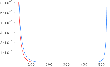
Figure 2.1: Plot of the near-core solution $y(\rho)=K_{0}(\sqrt{\lambda xe^{2x}})$ ($x=\log\rho/\rho_{L}$) and the exact solution $y(\rho)$ for $N_{f}=1$, $q=0.1$. The near-core solution breaks down around $\rho_{L}$.

$\rho$

$y(\rho)$

$\rho_{L}$

$K_{0}$

$/$

2.3 The decoupling limit and regime of validity

We shall now discuss the regime of validity of the supergravity solution. As mentioned earlier, it is in principle possible to find a (numerical) solution to the full D3/D7 configuration using the complete axion-dilaton of the D7-branes. Our background (2.1, 2.2, 2.6) approximates this solution in the regime

$$0\ll\rho\ll\rho_{L}\,.$$ (2.35)

This regime is bounded from above due to the naked singularity at $\rho_{L}$, where the dilaton diverges. The other limit is basically $\rho=0$, where the space has a curvature singularity due to the presence of the D7-branes. At this point the string coupling goes to zero which corresponds to the fact that the dual field theory becomes free in the infrared.

The decoupling limit is obtained as follows. The massless open string degrees of freedom correspond to a ${\cal N}=4$ super-Yang-Mills multiplet (3-3 strings) coupled to $N_{f}$ bifundamental ${\cal N}=2$ hypermultiplets (3-7 strings) localized at the $3+1$ dimensional intersection. We take a limit in which the 7-7 strings decouple, leaving a purely four-dimensional theory. This decoupling is achieved by taking a large $N_{c}$ limit while keeping the four-dimensional ’t Hooft coupling $\lambda=g^{2}_{YM}N_{c}\sim g_{s}N_{c}$ and $N_{f}$ fixed. This is the usual ’t Hooft limit for the gauge theory describing the $N_{c}$ D3-branes. The eight-dimensional ’t Hooft coupling $\lambda^{\prime}$ for the $N_{f}$ D7-branes is $\lambda^{\prime}=\lambda(2\pi l_{s})^{4}N_{f}/N_{c}$ which vanishes in the $\alpha^{\prime}\rightarrow 0$ limit. This turns the $SU(N_{f})$ gauge group on the D7-branes into a global flavor group.

Moreover, we take the limit of large ’t Hooft coupling. Then, the near-horizon geometry is obtained, as usual, by dropping the “1” in the warp factor $h(r,\rho)$. Writing $g_{s}e^{\Psi}=1-\nu\lambda\log\rho/\rho_{L}$ with $\nu=N_{f}/N_{c}$, one can easily see that in the strict $\nu\rightarrow 0$ limit, the near horizon geometry reduces to $AdS_{5}\times S^{5}$ with embedded probe D7-branes [1]. Recall that in this limit the warp factor (2.34) reduces to the harmonic function of the D3-branes. In other words, the background includes corrections to the quenched approximation of first order in $N_{f}/N_{c}$. In the field theory these corrections correspond to Feynman diagrams with empty quark loops.

The solution seems to be valid for any number of flavors. Neither the perturbative field theory nor the supergravity solution imposes any constraint on the number of flavors. Note, however, that a D7-brane solution, which extends to $\rho\rightarrow\infty$, is known to exist only for $N_{f}\leq 12$. It is therefore not clear, whether our D3/D7 solution can be extended to a full solution in the case of more than $12$ flavors. It should be safe to use it for $N_{f}\leq 12$, in which case the solution can in principle be numerically continued to infinity.

2.4 The warp factor of a fractional D3/D7 brane system

As a bonus for finding the warp factor for the D3/D7 brane system in flat space, we can actually construct the warp factor of another system, that of fractional D3/D7 branes on the orbifold $\mathbb{R}^{5,1}\times\mathbb{C}^{2}/\mathbb{Z}_{2}$, where the $\mathbb{Z}_{2}$ action is a reflection parity along the $x^{4},\dots x^{7}$ coordinates. The D3-branes span the $x^{0},\dots x^{3}$ coordinates and the D7-branes are oriented entirely along the orbifold, spanning $x^{0},\dots x^{7}$. Due to this fact, the D7-branes also source, beside the axion-dilaton, a twisted scalar and a twisted 4-form potential. Their charge is half that of ordinary D7-branes, for which reason they are called fractional D7 branes. The system whose warp factor we will construct next is composed of $N_{f}$ fractional D7-branes and $N_{c}$ fractional D3-branes [38]. The warp factor has been known so far only in terms of the differential equation

$$(\Box_{4}+e^{-\phi}\Box_{2})H + 2\kappa^{2}_{orb}\tau_{3}N_{c}\delta(x^{4})\dots\delta(x^{9})$$ (2.36)

$$+ (2\pi\alpha^{\prime}g_{s})^{2}\frac{(2N_{c}-N_{f}/2)^{2}}{\rho^{2}(1-N_{f}g_{s}/(2\pi)\ln(\rho/\epsilon))^{3}}\delta(x^{4})\dots\delta(x^{7})=0\,,$$

where $\tau_{3}$ is the tension of the fractional D3-brane, $\Box_{4}$ denotes the four-dimensional flat space Laplacean along the directions $\{x^{4}\dots x^{7}\}=\{\vec{r}\}$ and $\Box_{2}$ is the two-dimensional flat space Laplacean along the directions $\{x^{8},x^{9}\}\equiv\{\vec{\rho}\}$. Also, the dilaton is

$$e^{-\phi}=1-\frac{N_{f}g_{s}}{2\pi}\ln\bigg{(}\frac{\rho}{\epsilon}\bigg{)}\,.$$ (2.37)

We recognize the differential operator acting on the warp factor being the same as the one whose Green’s function we have computed previously

$$G(\rho,\varphi;\vec{r};\rho^{\prime},\varphi^{\prime},\vec{r}^{\prime})=\frac{C}{(2\pi)^{5}}\sum_{l}\int d^{4}\vec{q}e^{i\vec{q}(\vec{r}-\vec{r}^{\prime})}e^{il(\varphi-\varphi^{\prime})}\tilde{y}_{l,q}(\rho_{<})y_{l,q}(\rho_{>})\,,$$ (2.38)

where $\vec{\rho}=\{\rho,\varphi\}$, $\rho_{<}=min(\rho,\rho^{\prime})$, $\rho_{>}=max(\rho,\rho^{\prime})$, and $\tilde{y}_{l,q}(\rho_{<})$ is the GP solution, well behaved at the origin, and $y_{l,q}(\rho_{>})$ is the generalization of the solution discussed in App. B. Therefore, the full warp factor of the fractional D3/D7 system is given by

$$H(\vec{\rho},\vec{r}) = 1-\int d^{4}\vec{r}^{\prime}\int d^{2}\vec{\rho}^{\prime}G(\vec{\rho},\vec{r};\vec{\rho}^{\prime},\vec{r}^{\prime})\bigg{[}2\kappa^{2}_{orb}\tau_{3}N_{c}\delta^{4}(\vec{r}^{\prime})\delta^{2}(\vec{\rho}^{\prime})$$ (2.39)

$$+ (2\pi\alpha^{\prime}g_{s})^{2}\frac{(2N_{c}-N_{f}/2)^{2}}{|\vec{\rho}^{\prime}|^{2}(1-N_{f}g_{s}/(2\pi)\ln(|\vec{\rho}^{\prime}|/\epsilon))^{3}}\delta^{4}(\vec{r}^{\prime})\bigg{]}$$

with the numerical constant $C=-1$ fixed by requiring that the discontinuities of Eq. (2.36) at $\rho=\rho^{\prime}$ match on both sides. It is worth saying that the dual gauge theory of this supergravity background is an $d=4,{\cal N}=2$ supersymmetric Yang-Mills theory, with $SU(N_{c})$ gauge group and $N_{f}$ fundamental hypermultiplets. The orbifold action has projected out the adjoint hypermultiplet of the gauge theory dual to an ordinary D3/D7 system, leaving a gauge theory with a negative beta function for $N_{f}<2N_{c}$. This means that the fractional D3/D7 supergravity background with a logarithmically running axion-dilaton is dual to the ${\cal N}=2$ gauge theory at energies above the scale where the gauge coupling diverges and where non-perturbative effects become important.

2.5 The dual ${\cal N}=2$ field theory

The ${\cal N}=2$ field theory dual to the near-horizon geometry of the D3/D7 configuration in flat space has been studied in [1, 6]. This theory has $U(N_{c})$ gauge group and the field content of ${\cal N}=4$ super Yang-Mills and $N_{f}$ hypermultiplets in the fundamental representation. The global symmetry of the theory is $SO(4)\approx SU(2)_{\Phi}\times SU(2)_{\cal R}$ which consists of an $SU(2)_{\Phi}$ global symmetry rotating the scalars in the adjoint hypermultiplet and an $SU(2)_{\cal R}$ ${\cal N}=2$ R-symmetry. In the case of overlapping D3 and D7-branes, the fundamentals are massless and the theory has an additional $U(1)_{\cal R}$ R-symmetry.

We are interested in how far the supergravity background reflects the perturbative aspects of the gauge theory. The exact perturbative ${\cal N}=2$ beta function is given by

$$\beta_{{\cal N}=2} \equiv\mu\frac{d}{d\mu}\alpha=-\frac{\alpha^{2}}{2\pi}\left[2T_{G}-T_{\rm adj}-N_{f}T_{\rm fund}\right]=\beta_{{\cal N}=4}+\frac{\alpha^{2}}{2\pi}N_{f}=\frac{\alpha^{2}}{2\pi}N_{f}\,,$$ (2.40)

where $\alpha=g^{2}_{YM}/4\pi$, $T_{G}=N_{c}$, $T_{\rm adj}=2T_{G}$, $T_{\rm fund}=1$ and $\beta_{{\cal N}=4}=0$. In the ’t Hooft limit, the theory is considered at large $N_{c}$ with $g_{YM}$ small such that the ’t Hooft coupling $\lambda=g^{2}_{YM}N_{c}$ remains fixed. In this limit a much more meaningful quantity is the beta function of the ’t Hooft coupling

$$\beta^{\lambda}_{{\cal N}=2}\equiv N_{c}\beta_{{\cal N}=2}=\frac{1}{2\pi}\left(\frac{\lambda}{4\pi}\right)^{2}\frac{N_{f}}{N_{c}}\,.$$ (2.41)

We see that if $N_{f}/N_{c}$ is kept fixed, then the field theory is neither conformal nor asymptotically free. The theory is however conformal in the strict $N_{c}\rightarrow\infty$ limit [1].

A positive beta function leads to a running gauge coupling $g_{YM}$ which is given by

$$\alpha(Q^{2})=\frac{1}{\frac{\beta_{0}}{4\pi}\log\frac{\Lambda^{2}_{L}}{Q^{2}}}\qquad{\textmd{with}}\qquad\Lambda^{2}_{L}=\mu^{2}\exp\left(\frac{4\pi}{\beta_{0}\alpha(\mu^{2})}\right)\,,$$ (2.42)

$Q^{2}$ the energy scale, $\mu^{2}$ a reference scale and $\beta_{0}=N_{f}$. $\Lambda_{L}$ is the scale of the Landau pole at which the gauge coupling becomes divergent.

This can be compared with the action for a probe D3-brane placed in the D3/D7 supergravity background (2.1, 2.2, 2.6),

$$S_{D3} =-T_{D3}\int d^{4}\sigma e^{-\Phi}\sqrt{-\det(g_{ab}+{\cal F}_{ab})}+T_{D3}\int C^{4}+C^{0}{\cal F}\wedge{\cal F}$$

$$\approx T_{D3}\int d^{4}\sigma(2\pi\alpha^{\prime})^{2}\left[-\frac{1}{4}e^{-\Phi}F_{ab}F^{ab}+\chi F_{ab}\tilde{F}^{ab}\right]+...\,,$$ (2.43)

where ${\cal F}_{ab}=(2\pi\alpha^{\prime})F_{ab}$. Here we expanded to second order in the field strength and kept only terms relevant for the field theory. The axion $C^{0}=\chi$ and the dilaton are given by the complex structure (A.5). They are

$$\chi=\frac{N_{f}}{2\pi}\varphi\,,\qquad e^{-\Phi}={\frac{N_{f}}{4\pi}\log\frac{\rho^{2}_{L}}{\rho^{2}}}\,.$$ (2.44)

The D3-brane action relates the dilaton and the axion to the gauge coupling $g_{YM}^{2}=4\pi e^{\Phi}$ and theta angle $\theta_{YM}=2\pi\chi$. Upon identifying also $\alpha(Q^{2})=g^{2}_{YM}(Q^{2})/4\pi$, $\alpha(\mu^{2})=g^{2}_{YM}(\mu^{2})/4\pi=g_{s}$, $Q^{2}=\rho^{2}/(2\pi\alpha^{\prime}{}^{2})$, $\Lambda_{L}=\rho_{L}/(2\pi\alpha^{\prime}{}^{2})$, the running of the gauge coupling (2.42) follows from the logarithmic behavior of the dilaton, and the Landau pole $(g_{YM}\to\infty)$ is related to the dilaton divergence at

$$\rho_{L}=e^{\frac{2\pi}{g_{s}N_{f}}}=e^{\frac{2\pi N_{c}}{\lambda N_{f}}}\,.$$ (2.45)

This shows that both sides of the duality show the same pathology: The perturbative field theory becomes strongly coupled at the Landau pole $\Lambda_{L}$, while the supergravity solution breaks down at some distance $\rho_{L}$.

Furthermore, the $U(1)_{\cal R}$ chiral anomaly in the field theory is reflected by a nontrivial axion profile in the supergravity background. The instanton term in (2.43) correctly reproduces the Yang-Mills theta angle $\theta_{YM}=2\pi\chi={N_{f}}\varphi$. This corresponds to the breaking of the classical $U(1)_{\cal R}$ symmetry to $\mathbb{Z}_{2N_{f}}$ at the quantum level.

This shows that the solution (2.1, 2.2, 2.6) of the D3/D7 system perfectly reflects the perturbative aspects of the dual ${\cal N}=2$ field theory.

2.6 Logarithmic tadpoles and one-loop vacuum amplitudes

Since D7-branes are codimension-two branes, we expect uncanceled tadpoles in the string background. Tadpole divergences usually correspond to gauge anomalies and indicate an inconsistency in the theory. However, as it was found first in [33], logarithmic tadpoles do not correspond to gauge anomalies, but reflect the fact that the dual gauge theory is not conformal invariant. In fact, as we will show now following arguments given in [34], such tadpoles provide the correct one-loop running of the gauge coupling.

This can be seen by considering the one-loop annulus diagram of an open string stretching between the stack of D7-branes and a D3-brane dressed with an external background $SU(N_{c})$ gauge field. In the field theory limit this vacuum amplitude reduces to the one-loop diagrams determining the running of the gauge coupling [34]. When expanded to quadratic order in the gauge field, the amplitude reads:

$$Z_{37}=\frac{N_{f}}{(4\pi)^{2}}\int d^{4}x\left[-\frac{1}{4}\left(F^{a}_{\mu\nu}F^{a\mu\nu}-iF^{a}_{\mu\nu}\tilde{F}^{a\mu\nu}\right)\right]\int_{1/(\alpha^{\prime}\Lambda^{2})}^{\infty}\frac{d\tau}{\tau}e^{-\frac{\rho^{2}\tau}{2\pi\alpha^{\prime}}}\,.$$ (2.46)

The integral over $\tau$ is logarithmically divergent for small $\tau$ and has been regularized by an ultraviolet cut-off $\Lambda$. The parameter $\rho$ is the distance between the dressed D3-brane and the D7-branes. Threshold corrections to the amplitude (2.46), coming from massive string states, are absent in the $\alpha^{\prime}\rightarrow 0$ limit.

From the annulus amplitude, one deduces the gauge coupling

$$\frac{1}{g_{YM}^{2}}=\frac{N_{f}}{(4\pi)^{2}}\int_{1/(\alpha^{\prime}\Lambda^{2})}^{\infty}\frac{d\tau}{\tau}e^{-\frac{\rho^{2}\tau}{2\pi\alpha^{\prime}}}=\frac{N_{f}}{(4\pi)^{2}}\log\frac{\Lambda^{2}}{Q^{2}}\,,$$ (2.47)

where we defined the energy scale $Q^{2}=\rho^{2}/(2\pi\alpha^{\prime}{}^{2})$. The previous relation agrees with Eq. (2.42) and the dilaton behavior described by (2.44). This shows that tadpoles provide the correct one-loop running of the gauge coupling.

Furthermore, from the instanton term in (2.46), we may also extract the $\theta_{\rm YM}$ angle,

$$\theta_{\rm YM}=N_{f}\varphi\,,$$ (2.48)

where $\varphi$ is the phase of the complex coordinate $z=\rho e^{i\varphi}$ transverse to the D7-branes. As mentioned above, in the supergravity background the chiral anomaly is encoded in the axion $\chi$.

Under open/closed string duality, one can consider the above one-loop amplitude also as a tree-level closed string amplitude which encodes information about the supergravity solution. The absence of threshold corrections, i.e. massive open string state contributions to the gauge coupling, guarantees that open massless string states are precisely mapped into massless closed string states. The supergravity solution constructed in this paper is therefore sufficient to describe the perturbative field theory. Even though the dual string background has logarithmic divergences, it is still consistent as far as the description of the embedded non-conformal field theory is concerned.

Finally, it should be clear that in the conformal limit $N_{f}/N_{c}\rightarrow 0$, considered by Karch and Katz [1], the gauge coupling does not run, and by the above arguments, tadpoles are absent. Certainly, D7-branes which do not backreact on the geometry do not emit flux and there is no net charge.

3 Regge trajectories in the D3/D7 theory

As an application of our supergravity solution, we now discuss the general structure of Regge trajectories in the ${\cal N}=2$ gauge theory of the D3/D7 system by means of a semi-classical string computation. This will provide interesting information about the behavior of the Regge trajectories in dependence of the number of flavors. We shall compare our results with a similar analysis performed in the probe approximation in [2].

3.1 Spinning strings in the D3/D7 background

Following [39, 2, 9], we consider an open string rotating in the near-horizon limit of the D3/D7 background. We parameterize the four-dimensional spacetime part of our background (2.1, 2.2, 2.6) as

$$dx^{\mu}dx_{\mu} =-dt^{2}+dR^{2}+R^{2}d\varphi^{2}+dz^{2}\,,$$ (3.1)

where $R$ and $\varphi$ are the coordinates of the plane of rotation. The string has length $2R_{0}$ and stretches from $-R_{0}$ to $+R_{0}$ along the $R$ direction. The end points of the string are attached to an additional probe D7-brane located a distance $\rho_{R}$ away from the stack of D7-branes. Recall that we have to choose $\rho_{R}$ in the regime $0\ll\rho_{R}\ll\rho_{L}$, i.e. far away from the singularity at the location of the stack of D7-branes and from the dilaton divergence at $\rho_{L}$. An example of a spinning string is shown in Fig. 3.1.

In the field theory the set-up corresponds to $N_{f}$ massless flavors plus an additional massive flavor whose mass is proportional to $\rho_{R}$. In this theory we consider a meson, which consists of massive flavors, in the presence of $N_{f}$ massless flavors. We assume a large spin for the meson which allows a classical treatment of the dual spinning string. Recall that meson operators with large spin have small anomalous dimensions and quantum corrections are negligible [39].

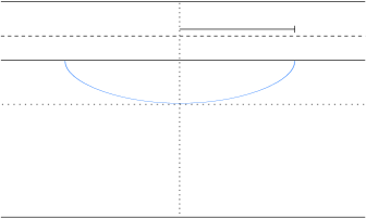
Figure 3.1: Example of a string profile $\tilde{z}(\tilde{R})$.

$\tilde{z}=\infty$ $(\rho=0)$                                                                              D7 stack

$\tilde{z}_{0}$

$\tilde{z}_{R}=\omega/\rho_{R}$                                                                                    probe D7

$\tilde{z}_{L}=\omega/\rho_{L}$                                                                                    dilaton singularity

$\tilde{z}=0$ $(\rho=\infty)$

boundary

$\tilde{R}_{0}(\omega)$

An appropriate ansatz for a string rotating with constant angular velocity $\omega$ is

$$t=\tau,\quad\varphi=\omega\tau,\quad R=R(\sigma),\quad r=r(\sigma),\quad\rho=\rho(\sigma)\,,$$ (3.2)

with world sheet coordinates $\sigma$ and $\tau$. With this ansatz the classical Nambu-Goto action takes the form

$${\cal L}=-T_{s}\sqrt{(1-\omega^{2}R^{2})(h^{-1}R^{\prime}{}^{2}+r^{\prime}{}^{2}+(1-\frac{N_{f}}{2\pi}\log\rho)\rho^{\prime}{}^{2})}\,.$$ (3.3)

It is convenient to use the rescaled coordinates

$$\tilde{R}=\omega R\,,\quad\tilde{r}=\frac{r}{\omega}\,,\quad\tilde{\rho}=\frac{\rho}{\omega}\,.$$ (3.4)

In these coordinates, the energy and the angular momentum of the spinning string are given by

$$E =\int d\sigma\left(\omega\frac{\partial{\cal L}}{\partial\omega}-{\cal L}\right)=\int d\sigma\frac{\omega}{\cal E}\sqrt{\tilde{h}^{-1}\tilde{R}^{\prime}(\sigma){}^{2}+\tilde{r}^{\prime}(\sigma)^{2}+e^{\psi}\tilde{\rho}^{\prime}(\sigma)^{2}}\,,$$ (3.5)

$$J =\int d\sigma\frac{\partial{\cal L}}{\partial\omega}=\int d\sigma\frac{\tilde{R}^{2}}{\cal E}\sqrt{\tilde{h}^{-1}\tilde{R}^{\prime}(\sigma)^{2}+\tilde{r}^{\prime}(\sigma)^{2}+e^{\psi}\tilde{\rho}^{\prime}(\sigma)^{2}}\,,$$ (3.6)

with ${\cal E}=\sqrt{1-\tilde{R}^{2}}$, $T_{s}=1$ and

$$\tilde{h}(\tilde{r},\tilde{\rho})=\frac{Q_{D3}}{(\tilde{r}^{2}+\tilde{\rho}^{2}e^{\Psi(\tilde{\rho})})^{2}}\,.$$ (3.7)

In the gauge $\tilde{R}=\sigma$, we find the following equations of motion for $\tilde{r}(\tilde{R})$ and $\tilde{\rho}(\tilde{R})$:

$$\frac{d}{d\tilde{R}}\left(\frac{{\cal E}^{2}}{\cal L}\partial_{\tilde{R}}\tilde{r}\right) =\frac{{\cal E}^{2}}{2{\cal L}}\partial_{\tilde{r}}\tilde{h}^{-1},$$ (3.8)

$$\frac{d}{d\tilde{R}}\left(\frac{{\cal E}^{2}}{{\cal L}}e^{\Psi}\partial_{\tilde{R}}\tilde{\rho}\right) =\frac{{\cal E}^{2}}{2{\cal L}}\left(\partial_{\tilde{\rho}}\tilde{h}^{-1}+(\partial_{\tilde{R}}\tilde{\rho})^{2}\partial_{\tilde{\rho}}e^{\Psi}\right)\,.$$ (3.9)

The warp factor $\tilde{h}(\tilde{r},\tilde{\rho})$ satisfies $\partial_{\tilde{r}}\tilde{h}^{-1}=0$ for $\tilde{r}=0$ which shows that $\tilde{r}\equiv 0$ is a solution of the equation of motion (3.8). Writing Eq. (3.9) in coordinates $\tilde{z}=1/\tilde{\rho}$, we find

$$\frac{d}{d\tilde{R}}\left(\frac{{\cal E}^{2}}{{\cal L}}e^{\Psi}\partial_{\tilde{R}}\tilde{z}^{-1}\right)=-\frac{{\cal E}^{2}}{2{\cal L}}\tilde{z}^{2}\left(\partial_{\tilde{z}}\tilde{h}^{-1}+(\partial_{\tilde{R}}\tilde{z}^{-1})^{2}\partial_{\tilde{z}}e^{\Psi}\right)\,.$$ (3.10)

This is a nonlinear differential equation of second order which requires two boundary conditions. We impose the usual open string boundary conditions

$$\left.\frac{\partial{\cal L}}{\partial\tilde{R}^{\prime}}\delta\tilde{R}\right|_{\sigma=0,\pi}=\left.\frac{\partial{\cal L}}{\partial\tilde{z}^{\prime}}\delta\tilde{z}\right|_{\sigma=0,\pi}=0\,$$ (3.11)

for a string ending on a probe D7-brane at $\tilde{z}=\tilde{z}_{R}=const$. Due to the Neumann boundary condition in the $\tilde{R}$ direction and the Dirichlet boundary condition in the $\tilde{z}$ direction, $\delta\tilde{R}|_{\sigma=0,\pi}$ is arbitrary, whereas $\delta\tilde{z}|_{\sigma=0,\pi}=0$. The remaining condition $\partial{\cal L}/{\partial\tilde{R}^{\prime}}|_{\sigma=0,\pi}=0$ is satisfied, if $\tilde{R}^{\prime}|_{\sigma=0,\pi}=0$. Using the gauge $\tilde{z}=\sigma$, we see that this corresponds to ${\partial\tilde{z}}/{\partial\tilde{R}}|_{\tilde{R}=\pm\tilde{R}_{0}}\rightarrow\infty$. This means that the string ends orthogonally on $\tilde{z}_{R}$.

We expect the solutions to be symmetric around $\tilde{R}=0$, where they have their only maximum. We thus impose the additional boundary condition $\tilde{z}^{\prime}(0)=0$. Taking into account the orthogonal ending of the string on a constant value of $\tilde{z}$, we set $\tilde{z}(\pm\tilde{R}_{0})=\tilde{z}_{R}=const.$ or, equivalently, $\tilde{z}(0)=\tilde{z}_{0}=const$.

3.2 Dependence of Regge trajectories on the number of flavors

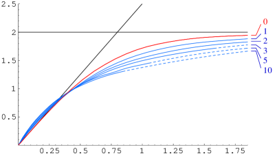
Figure 3.2: Chew-Frautschi plot for $N_{f}=0,1,2,3,5,10$ additional massless flavors. The straight line represents the $N_{f}=0$ trajectory for small spin values. All graphs approach the horizontal line $E=2m$.

$\sqrt{J}/\lambda^{1/4}$

$E/m$

The Regge trajectories $E(J;N_{f})$ can now be obtained as follows. We first solve the equation of motion (3.10) for the string profile $\tilde{z}(\tilde{R})$. We then substitute the profile into the expressions (3.5) and (3.6) for the energy $E(\omega)$ and the angular momentum $J(\omega)$ of the spinning string. This yields a Regge trajectory as a curve in the $\sqrt{J},E$ plane parameterized by the angular velocity $\omega$.

We begin by fixing the mass $m$ of the single flavor corresponding to a 3-7 string stretching from the D3-branes at $\rho=0$ ($\tilde{z}\rightarrow\infty$) to the probe D7-brane at $\tilde{z}_{R}=\omega/\rho_{R}$:

$$m=\int_{\varepsilon}^{\rho_{R}}\sqrt{g_{00}g_{\rho\rho}}d\rho=\int_{\varepsilon}^{\rho_{R}}e^{\Psi/2}d\rho=\int_{\varepsilon}^{\rho_{R}}(\frac{1}{g_{s}}-\frac{N_{f}}{2\pi}\log\rho)^{1/2}d\rho\,,$$ (3.12)

where $\varepsilon\ll 1$ is a (IR) cut-off which is needed to regularize the singularity at $\rho=0$. We set $m=1$ and solve this equation numerically for $\rho_{R}(m,N_{f})$. In this way we obtain the location of the probe D7-brane $\tilde{z}_{R}(m,N_{f})=\omega/\rho_{R}(m,N_{f})$. The set of Regge trajectories in Fig. 3.2 is obtained by varying $\omega$ for a given number of massless flavors $N_{f}$, then changing $N_{f}$ while all the time keeping the mass $m$ fixed.

We now determine the string profile $\tilde{z}_{R}$ for given $N_{f}$ and $\omega$. To this end, we integrate the equations of motion (3.10) from $-\tilde{R}_{0}$ to $+\tilde{R}_{0}$. In the shooting technique, we set $\tilde{z}(0)=\tilde{z}_{0}=const$, $\tilde{z}^{\prime}(0)=0$ such that $\tilde{z}(\pm\tilde{R}_{0})=\tilde{z}_{R}$. This yields the string length $R_{0}=\tilde{R}_{0}/\omega$ as the location at which $\tilde{z}^{\prime}(\tilde{R}_{0})\rightarrow\infty$. A typical profile has been shown in Fig. 3.1.

Substituting the profiles $\tilde{r}(\tilde{R})\equiv 0$ and $\tilde{\rho}(\tilde{R})^{-1}=\tilde{z}(\tilde{R})$ into Eqns. (3.5) and (3.6), we determine the energy $E(\omega)$ and the angular momentum $J(\omega)$ in dependence of the angular velocity $\omega$. Repeating the procedure for different $\omega$, we obtain a parametric plot for the Regge trajectory $E(\sqrt{J};N_{f})$ associated with a certain number of flavors $N_{f}$.

In the computation we keep $g_{s}\sim\lambda/N_{c}$ small, but fixed such that the background depends on the small but finite parameter $\nu=N_{f}/N_{c}$.

Our results are presented in Fig. 3.2 which shows the Regge trajectories for different numbers of massless flavors $N_{f}$. The energy $E$ and the spin $J$ of the mesons are given in units of the quark mass $m$ and the square root of the ’t Hooft coupling $\lambda$, respectively. As a first check of our numerics, we note that the graph for $N_{f}=0$ coincides with that found in the probe limit [2]. Disregarding the behavior at small spin values, the graph for $N_{f}=0$ runs above the graphs for $N_{f}\neq 0$.

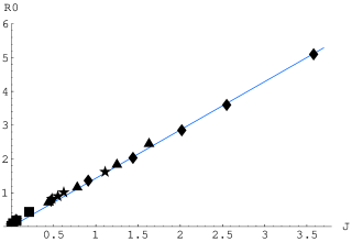
Figure 3.3: String length $R_{0}(J)$ for different $N_{f}$.

The semiclassical approximation is valid as long as the quantum effects are suppressed by $T_{s}/S_{cls}\ll 1$ where $S_{cls}=E/\omega-J$ is the value of the action evaluated on the classical solution. One can check that while the linear behavior of the Regge trajectories lies well outside the region of validity of the semiclassical approximation, the region where the quantum effects are suppressed is still sensitive to the number of flavors.

Let us first consider the general behavior of the Regge trajectories. Quite generically, the trajectories are linear in the small spin region and asymptote to the rest energy $E=2m$ in the large spin limit. This can be understood from the behavior of the string length as a function of the spin. Fig. 3.3 shows that the data fits a linear relation between the string length $R_{0}$ and the spin $J$. Note that this plot contains data from graphs for different $N_{f}$. Since the linear relation is the same for all $N_{f}$, we find that the string length $R_{0}$ does not depend on the number of massless flavors.

At small spin values the length of the string is much smaller than the scale of the space, $R_{0}\ll Q_{D3}$, and the string is effectively rotating in flat space leading to a linear Regge behavior. At large spin the string is larger than the size of the space, $R_{0}\gg Q_{D3}$. Here the string rotates very slowly and the energy is that of particles moving in a Coulomb potential [2]. Moreover, since the string length grows linearly with spin, also the binding energy of the quark-antiquark pair vanishes at large spin values. The Regge trajectories thus asymptote to the rest energy $E=2m$ in the limit $\omega\rightarrow 0$.

Let us now compare trajectories with different numbers of flavors. We observe that for a meson with fixed (large) spin, the energy is the lower the larger the number of flavors in the theory, i.e. $E_{1}>E_{2}$ for $N_{f}^{1}<N_{f}^{2}$ and $J_{1}=J_{2}$. In other words, the graph for smaller $N_{f}$ is above the graph for higher $N_{f}$ in the $\sqrt{J},E$ plane.

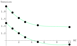
Figure 3.4: String tension in dependence of the number of flavors $N_{f}$ for $J=0.4^{2}$ (upper graph) and $J=0.6^{2}$ (lower graph).

To understand this behavior, it is illuminating to consider the string tension for a fixed spin value as a function of $N_{f}$. The square root of the tension is proportional to the derivative of $E(\sqrt{J})$. Fig. 3.4 shows that the string tension is a monotonically decreasing function of $N_{f}$. Since other quantities like the string length are unaffected by an increasing number of flavors, the energy of a meson is smaller in a theory with more flavors. This effect vanishes however at very large values of the spin.

The behavior of the string tension can also be understood in the dual field theory. The rotating string can be considered as a spin chain of gluons with quarks at the end of the string. In between the quark and the antiquark of the meson there are virtual quark-antiquark pairs which interact with the gluon chain. The polarization of these virtual quark-antiquark pairs effectively diminishes the color force between the quarks of the meson. This screening effect should have an influence on the string tension. We expect that a large number of flavors in a field theory leads to a small string tension. At least heuristically, this explains the fact that a meson with a certain spin has less energy than the same meson in a theory with a larger number of flavors.

Even though the background we are discussing is not confining, a similar effect is observed in lattice QCD with dynamical light quarks, where the interaction potential between two heavy quarks

$$V(r)=\left(-\frac{\alpha}{r}+\sigma r\right)\frac{1-e^{-\mu r}}{\mu r}$$ (3.13)

was a better fit to the data, rather than the unscreened potential [40]. For non-vanishing inverse screening length $\mu$, the effective flux tube tension between the heavy quarks is diminished due to the screening of the color charge, with $\mu$ increasing with the number of light quarks.

4 Conclusions

To summarize our results, we have completed the type IIB supergravity solution describing the fully localized D3/D7 brane configuration by providing an analytic expression for the warp factor. The background is given by the metric

$$ds_{10}^{2}=h^{-1/2}(r,\rho)\,dx_{\mu}^{2}+h^{1/2}(r,\rho)\left(dr^{2}+r^{2}d\Omega^{2}_{3}+e^{\Psi(\rho)}(d\rho^{2}+\rho^{2}d\varphi)\right)\,$$ (4.1)

for which we assumed a logarithmically running axion-dilaton:

$$\chi(\varphi)=\frac{N_{f}}{2\pi}\varphi\,,\qquad e^{-\phi(\rho)}=e^{\Psi(\rho)}=-\frac{N_{f}}{2\pi}\log\frac{\rho}{\rho_{L}}\,,\qquad\rho_{L}=e^{\frac{2\pi}{g_{s}N_{f}}}\,.$$ (4.2)

Upon taking the decoupling limit, this is the supergravity dual of ${\cal N}=4$ $SU(N_{c})$ super Yang-Mills gauge theory with $N_{f}$ ${\cal N}=2$ fundamental hypermultiplets.

The warp factor $h(r,\rho)$ is given in terms of a convergent series:

$$h(r,\rho) =1+Q_{D3}\int_{0}^{\infty}dq\frac{(qr)^{2}J_{1}(qr)}{2r^{3}}\sum_{n=0}^{\infty}\lambda^{n}e^{2nx}p_{n}(x)\,,\qquad x=\log(\rho/\rho_{L})\,,$$ (4.3)

where $\lambda=\frac{-N_{f}}{2\pi}\rho_{L}^{2}q^{2}$, and the polynomials $p_{n}(x)$ ($n=0,1,2,...$) are defined recursively by

$$\left(4n^{2}+4n\frac{d}{dx}+\frac{d^{2}}{dx^{2}}\right)p_{n} =xp_{n-1}\,,\qquad p_{0}(x)=-x-\log(\rho_{L}q/2)-\gamma\,.$$ (4.4)

In the immediate vicinity of the D7-branes, $x\rightarrow-\infty$ ($\rho\rightarrow 0$), the warp factor can be approximated by the simple expression

$$h(r,\rho)=1+\frac{Q_{D3}}{(r^{2}+\rho^{2}e^{\Psi(\rho)})^{2}}\,.$$ (4.5)

We have related the pathology of the supergravity background to the Landau pole of the gauge theory which has a positive beta function. We have also shown that the existence of a logarithmic tadpole in the one-loop open string amplitude between the D3 and D7-branes is related to the same one-loop running of the gauge coupling.

In the second part of this paper, we have considered classical spinning string configurations in the backreacted D3/D7 geometry and analyzed the dependence of the associated meson Regge trajectories on the number of flavors. From the Chew-Frautschi plots $(E,\sqrt{J})$ we have found that for the same spin, the energy of a meson is smaller in a gauge theory with more flavors. We interpreted this in terms of a screening effect of the color charge due to virtual $q\bar{q}$ pairs. Since the background is non-confining, in the IR, where the theory becomes conformal, the tension of the quark-antiquark flux tube vanishes at large spin $J$, and the meson configuration energy approaches the rest mass of its constituents.

We have seen that taking into account the backreaction of the flavor branes opens up the possibility of going beyond the quenched approximation via the AdS/CFT correspondence. An immediate goal would be the study of confining backgrounds, including the backreaction of the flavor branes. Also, it is well-known that $SU(N)$ gauge theories undergo a chiral phase transition [42] as the number of flavors is varied, even at zero temperature. It would be interesting if these phase transitions could be studied from the perspective of the dual supergravity background.

Appendix A Brief review of the D7-branes geometry

For completeness, we review here the geometry of a stack of D7-branes which has first been studied in [41] in the context of cosmic string solutions. The standard metric ansatz for the type IIB supergravity solution corresponding to a stack of $N_{f}$ coincident D7-branes is

$$ds_{10}^{2}=ds_{8}^{2}+e^{\Psi(z,\bar{z})}dzd\bar{z}\,,$$ (A.1)

where $ds^{2}_{8}$ is an eight-dimensional flat metric and $z$ is a complex coordinate parameterizing the space transverse to the D7-branes. D7-branes couple to the axion-dilaton field $\tau=\chi+ie^{-\phi}$.

The complex structure $\tau$ and the function $\Psi$ have to satisfy the equations of motion [41]

$$\partial\overline{\partial}\tau+\frac{2\partial\tau\overline{\partial}\tau}{\bar{\tau}-\tau}=N_{f}\delta(z)\,,$$ (A.2)

$$\partial\overline{\partial}\Psi=\partial\overline{\partial}\,\log{\,\rm Im\,}(\tau)\,.$$ (A.3)

The first equation requires $\tau$ to be holomorphic or anti-holomorphic. In order to have a finite string coupling, ${\rm Im}\,(\tau)$ must be nonzero for all values of $|z|$. The basic solution for $\tau$ can be written in terms of the modular invariant $j$-function [41]. A stack of $N_{f}$ D7-branes corresponds to a pole of order $N_{f}$ in the $j$-plane which can locally be parameterized by

$$j(\tau)=\frac{1}{(z/\rho_{L})^{N_{f}}}\,.$$ (A.4)

For small $|z|$, $j(\tau)$ is large and can be approximated by $\exp(-2\pi i\tau)$. Substituting $j\sim\exp(-2\pi i\tau)$ in Eq. (A.4) and solving for $\tau$, we get the weak-coupling approximation

$$\tau(z)=-i\frac{N_{f}}{2\pi}\log\left(\frac{z}{\rho_{L}}\right)\,.$$ (A.5)

The integration constant $\rho_{L}$ determines the string coupling.

The second equation of motion, Eq. (A.3) is solved by

$$e^{\psi(z,\bar{z})}=\Omega\bar{\Omega}{\,\rm Im\,}(\tau)\,,$$ (A.6)

where $\Omega$ is an arbitrary holomorphic function. This function is fixed by requiring modular invariance and regularity of the metric at the location of the D7-branes. The function $e^{\Psi}$ is thus given by

$$e^{\Psi(z,\bar{z})}=\tau_{2}(z)|\eta(\tau)|^{4}|z|^{-{N_{f}}/{6}}$$ (A.7)

with $\eta$ the Dedekind eta function and $\tau_{2}={\rm Im}\,(\tau)$. In the weak coupling region, $|z|\ll\rho_{L}$, $\tau_{2}$ is large and the function $e^{\Psi}$ is well-approximated by

$$e^{\Psi(z,\bar{z})}\approx\tau_{2}\,.$$ (A.8)

Asymptotically, for $|z|\gg\rho_{L}$, the complex structure $\tau$ as given by Eq. (A.4) approaches the constant $\tau=j^{-1}(0)$ and $e^{\Psi(z,\bar{z})}\approx|z|^{-N_{f}/6}$. This leads to an asymptotically flat metric with a deficit angle of $2\pi N_{f}/12$ as can be seen from the transverse part of the D7 metric,

$$ds^{2}_{\perp}=\rho^{-N_{f}/6}(d\rho^{2}+\rho^{2}d\varphi^{2})=\frac{1}{(1-\frac{N_{f}}{12})^{2}}(d\rho^{\prime}{}^{2}+\rho^{\prime}{}^{2}(1-\frac{N_{f}}{12})^{2}d\varphi^{2})\,,$$ (A.9)

where $\rho^{\prime}=\rho^{1-N_{f}/12}$. This shows that the transverse space is asymptotically conical for $N_{f}<12$ and asymptotically cylindrical for $N_{f}=12$. For $N_{f}>12$ the transverse space is compact and in general singular apart from the exceptional case $N_{f}=24$.

Appendix B Solving the equation (2.18)

The second order differential equation (2.18) admits two independent solutions. One of them, which is well behaved near $x=0$, was found by Gesztesy and Pittner [32]:

$$y(x)=\sum^{\infty}_{n=0}\lambda^{n}e^{2nx}p_{n}(x)\,,$$ (B.1)

where the polynomials $p_{n}(x)$ are defined by the recursion relation

$$\left(4n^{2}+4n\frac{d}{dx}+\frac{d^{2}}{dx^{2}}\right)p_{n}(x) =xp_{n-1}(x)\,,\qquad p_{0}(x)=1\,.$$ (B.2)

The series converges uniformly on the negative real line, $x<0$.

Here we proceed to derive the other independent solution which is needed in the construction of the warp factor of the backreacted D3/D7 geometry.

The recurrence relation

$$\bigg{(}4n^{2}+4n\frac{d}{dx}+\frac{d^{2}}{dx^{2}}\bigg{)}p_{n}(x)=xp_{n-1}(x)\,$$ (B.3)

can be decomposed into a set of algebraic equations for the expansion coefficients of the polynomials $p_{n}(x)$. With the initial condition

$$p_{0}(x)=ax+b\,,$$ (B.4)

where $a,b$ are constants, we find that

$$p_{n}(x)=\sum_{k=0}^{n+1}c^{(n)}_{k}x^{k}\,,$$ (B.5)

and where the coefficients $c^{(n)}_{k}$ satisfy the following system of equations

$$4n^{2}c_{n+1}^{(n)}=c_{n}^{(n-1)}\,,$$

$$4n^{2}c_{n}^{(n)}+4n(n+1)c_{n+1}^{(n)}=c_{n-1}^{(n-1)}\,,$$

$$4n^{2}c_{n-k}^{(n)}+4n(n-k+1)c_{n-k+1}^{(n)}+(n-k+2)(n-k+1)c_{n-k+2}^{(n)}=c_{n-k-1}^{(n-1)},\qquad k\geq 1$$

$$4n^{2}c_{0}^{(n)}+4nc_{1}^{(n)}+2c_{2}^{(n)}=0\,.$$ (B.6)

According to our initial condition, we have $c_{0}^{(0)}=b,c_{1}^{(0)}=a$. One can easily solve for the leading expansion coefficients (for $x\to-\infty$)

$$c_{n+1}^{(n)} = \frac{a}{4^{n}(n!)^{2}},\qquad c_{n}^{(n)}=\frac{b}{4^{n}(n!)^{2}}-\frac{a}{4^{n}(n!)^{2}}(n+\psi(n+1)+\gamma)$$

$$c_{n-1}^{(n)} = -\frac{1}{4n^{2}}\bigg{(}4n^{2}c_{n}^{(n)}+n(n+1)c_{n+1}^{(n)}+\frac{1}{4(n-1)^{2}}\bigg{(}$$ (B.7)

$$4(n-1)^{2}c_{n-1}^{(n-1)}+n(n-1)c^{(n-1)}_{n}+\frac{1}{4(n-2)^{2}}\bigg{(}$$

$$4(n-2)^{2}c_{n-2}^{(n-2)}+(n-1)(n-2)c_{n-1}^{(n-2)}+\dots\frac{1}{4}\bigg{(}4c^{(1)}_{1}+1\cdot 2c_{2}^{(1)}\bigg{)}\dots\bigg{)}$$

$$= -\frac{1}{4^{n}(n!)^{2}}\bigg{[}bn-a\bigg{(}\frac{4n+3}{4}(\psi(n+1)+\gamma)+\frac{n(2n-3)}{4}\bigg{)}\bigg{]}\,,$$

where $\psi(n)=\frac{d\ln\Gamma(x)}{dx}$ is the polygamma function, and $\gamma=-\psi(1)$ is the Euler-Mascheroni constant.

Let us show that in the limit when the number of flavors is set to zero (i.e. there are no D7-branes), we recover the modified Bessel function $K_{0}(q\rho)$ which is needed to reconstruct the warp factor of the geometry obtained by taking the near-horizon limit of a set of overlapping D3-branes (i.e. the Green’s function of the six-dimensional flat space Laplace equation).

We begin by reintroducing the initial set of variables

$$\lambda=-\frac{N_{f}}{2\pi}q^{2}e^{4\pi/N_{f}},\qquad x=\ln\rho-\frac{2\pi}{N_{f}}$$ (B.8)

which yield

$$y(x) = \sum(\lambda e^{2x})^{n}p_{n}(x)$$ (B.9)

$$= \sum\bigg{(}-\frac{N_{f}}{2\pi}\bigg{)}^{n}(q\rho)^{2n}\frac{1}{4^{n}(n!)^{2}}\bigg{[}a(\ln\rho-\frac{2\pi}{N_{f}})^{n+1}$$

$$+\bigg{(}b-a\bigg{(}n+\gamma+\psi(n+1)\bigg{)}\bigg{)}(\ln\rho-\frac{2\pi}{N_{f}})^{n}$$

$$+\bigg{(}bn-a(n+1)\bigg{(}\frac{(n+1)^{2}-7}{6}+\gamma+\psi(n+2)\bigg{)}\bigg{)}(\ln\rho-\frac{2\pi}{N_{f}})^{n-1}$$

$$+\dots\bigg{]}\,.$$

In order to obtain

$$K_{0}(q\rho)=\sum_{n=0}^{\infty}\frac{(q\rho)^{2n}(\psi(n+1)-\log(q\rho/2))}{4^{n}(n!)^{2}}\,,$$ (B.10)

we must choose

$$b=\frac{2\pi a}{N_{f}}+a\gamma+a\ln(q/2)\,.$$ (B.11)

Notice that with this choice we find that the only terms in the $x(\rho)$ expansion of $y(x)$ that contribute in the limit $N_{f}\to 0$ are at most of order $x^{n-1}$, and at this order, the only contribution comes from the $b$-dependent term. The $anN_{f}^{n}x^{n}$ term is now canceled upon taking $N_{f}\to 0$ by the $bnN_{f}^{n}x^{n-1}$ term. This completes the proof that $y(x(\rho))$ reduces indeed to $K_{0}(q\rho)$ when setting the number of flavors to zero. Moreover, the requirement that in this limit we obtain the modified Bessel function $K_{0}(q\rho)$, allowed us to enforce the relation (B.11) between the ab initio free parameters $a,b$. The remaining dependence on $a$ manifests as an overall proportionality coefficient which we fix by the same requirement that in the limit $N_{f}\to 0$ the solution $y(x(\rho))$ becomes $K_{0}(q\rho)$. From now on, we set $a=-1$ and (B.11).

The absolute value of the coefficients $c_{k}^{(n)}$ is bounded from above by

$$|c_{k}^{(n)}|\stackrel{{\scriptstyle<}}{{=}}\frac{1}{4^{n}n!}\bigg{(}|a|(\psi(n+1)+\gamma+1)C_{n+1}^{n+1-k}2^{n+1-k}+|b|C_{n}^{n-k}2^{n-k}\bigg{)}\,.$$ (B.12)

Consequently, the polynomials $p_{n}(x)$ obey the inequality

$$|p_{n}(x)|\stackrel{{\scriptstyle<}}{{=}}\frac{1}{4^{n}n!}\bigg{(}|a|(\psi(n+1)+\gamma+1)(2+|x|)^{n+1}+|b|(2+|x|)^{n}\bigg{)}\,.$$ (B.13)

Therefore it can be shown that the series $y(x)=\sum\lambda^{n}e^{2nx}p_{n}(x)$ is convergent given that each term in the series is smaller than the corresponding term of a convergent series $\sum|\lambda|^{n}e^{2nx}\frac{1}{4^{n}n!}\bigg{(}|a|(\psi(n+1)+\gamma+1)(2+|x|)^{n+1}+|b|(2+|x|)^{n}\bigg{)}$. The convergence of the latter series is proven by showing that the ratio of two consecutive terms $a_{n}/a_{n-1}=\lambda e^{x}(2+x)(|a|(2+|x|)(\psi(n)+\gamma+1)+|b|)/((a(2+|x|)(\psi(n-1)+\gamma+1)+|b|)4n)$ approaches zero as $n\to\infty$.

References

- [1] A. Karch and E. Katz, JHEP 0206, 043 (2002) [arXiv:hep-th/0205236].
- [2] M. Kruczenski, D. Mateos, R. C. Myers and D. J. Winters, JHEP 0307, 049 (2003) [arXiv:hep-th/0304032].
- [3] T. Sakai and J. Sonnenschein, JHEP 0309, 047 (2003) [arXiv:hep-th/0305049].
- [4] P. Ouyang, Nucl. Phys. B 699, 207 (2004) [arXiv:hep-th/0311084].
- [5] C. Nunez, A. Paredes and A. V. Ramallo, JHEP 0312, 024 (2003) [arXiv:hep-th/0311201].
- [6] S. Hong, S. Yoon and M. J. Strassler, JHEP 0404, 046 (2004) [arXiv:hep-th/0312071].
- [7] S. Hong, S. Yoon and M. J. Strassler, arXiv:hep-th/0409118.
- [8] J. Erdmenger and I. Kirsch, JHEP 0412, 025 (2004) [arXiv:hep-th/0408113].
- [9] M. Kruczenski, L. A. P. Zayas, J. Sonnenschein and D. Vaman, arXiv:hep-th/0410035.
- [10] A. Paredes and P. Talavera, Nucl. Phys. B 713, 438 (2005) [arXiv:hep-th/0412260].
- [11] G. F. de Teramond and S. J. Brodsky, arXiv:hep-th/0501022.
- [12] G. Siopsis, arXiv:hep-th/0503245.
- [13] J. Babington, J. Erdmenger, N. J. Evans, Z. Guralnik and I. Kirsch, Phys. Rev. D 69, 066007 (2004) [arXiv:hep-th/0306018].
- [14] J. Babington, J. Erdmenger, N. J. Evans, Z. Guralnik and I. Kirsch, Fortsch. Phys. 52, 578 (2004) [arXiv:hep-th/0312263].
- [15] M. Kruczenski, D. Mateos, R. C. Myers and D. J. Winters, JHEP 0405, 041 (2004) [arXiv:hep-th/0311270].
- [16] N. J. Evans and J. P. Shock, Phys. Rev. D 70, 046002 (2004) [arXiv:hep-th/0403279].
- [17] J. L. F. Barbon, C. Hoyos, D. Mateos and R. C. Myers, JHEP 0410, 029 (2004) [arXiv:hep-th/0404260].
- [18] I. Kirsch, Fortsch. Phys. 52, 727 (2004) [arXiv:hep-th/0406274].
- [19] K. Ghoroku and M. Yahiro, Phys. Lett. B 604, 235 (2004) [arXiv:hep-th/0408040].
- [20] T. Sakai and S. Sugimoto, Prog. Theor. Phys. 113, 843 (2005) [arXiv:hep-th/0412141].
- [21] D. Bak and H. U. Yee, Phys. Rev. D 71, 046003 (2005) [arXiv:hep-th/0412170].
- [22] L. Da Rold and A. Pomarol, arXiv:hep-ph/0501218.
- [23] N. Evans, J. Shock and T. Waterson, JHEP 0503, 005 (2005) [arXiv:hep-th/0502091].
- [24] R. Apreda, J. Erdmenger, N. Evans and Z. Guralnik, arXiv:hep-th/0504151.
- [25] S. A. Cherkis and A. Hashimoto, JHEP 0211, 036 (2002) [arXiv:hep-th/0210105].
- [26] H. Nastase, arXiv:hep-th/0305069.
- [27] A. Kehagias, Phys. Lett. B 435, 337 (1998) [arXiv:hep-th/9805131].
- [28] O. Aharony, A. Fayyazuddin and J. M. Maldacena, JHEP 9807, 013 (1998) [arXiv:hep-th/9806159].
- [29] M. Grana and J. Polchinski, Phys. Rev. D 65, 126005 (2002) [arXiv:hep-th/0106014].
- [30] B. A. Burrington, J. T. Liu, L. A. Pando Zayas and D. Vaman, JHEP 0502, 022 (2005) [arXiv:hep-th/0406207].
- [31] J. T. Liu, D. Vaman and W. Y. Wen, arXiv:hep-th/0412043.
- [32] F. Gesztesy and L. Pittner, J. Phys. A 11, 679 (1978).
- [33] R. G. Leigh and M. Rozali, Phys. Rev. D 59, 026004 (1999) [arXiv:hep-th/9807082].
- [34] P. Di Vecchia, A. Liccardo, R. Marotta and F. Pezzella, arXiv:hep-th/0503156; P. Di Vecchia, A. Liccardo, R. Marotta and F. Pezzella, JHEP 0306, 007 (2003) [arXiv:hep-th/0305061].
- [35] K. Dasgupta, C. Herdeiro, S. Hirano and R. Kallosh, Phys. Rev. D 65, 126002 (2002) [arXiv:hep-th/0203019].
- [36] Lisa Randall, private communication; Lisa Randall, “Relaxing to Three Dimensions” on work with Andreas Karch, Talk given at Harvard University, April 8, 2005; see also “http://motls.blogspot.com/2005/04/lisa-randalls-talk.html” for a report on the talk by Lubo Motl.
- [37] D. Lüst, P. Mayr, S. Reffert and S. Stieberger, arXiv:hep-th/0501139.
- [38] M. Bertolini, P. Di Vecchia, M. Frau, A. Lerda and R. Marotta, Nucl. Phys. B 621, 157 (2002) [arXiv:hep-th/0107057].
- [39] S. S. Gubser, I. R. Klebanov and A. M. Polyakov, Nucl. Phys. B 636, 99 (2002) [arXiv:hep-th/0204051].
- [40] K. D. Born, E. Laermann, N. Pirch, T. F. Walsh, P. M. Zerwas, Phys. Rev. D40, 1653 (1989)
- [41] B. R. Greene, A. D. Shapere, C. Vafa and S. T. Yau, Nucl. Phys. B 337, 1 (1990).
- [42] T. Appelquist, J. Terning and L. C. R. Wijewardhana, Phys. Rev. Lett. 77 (1996) 1214 [arXiv:hep-ph/9602385].