hep-th/0505099

PUPT-2160

ITEP-TH-33/05

Perturbative Search for Fixed Lines

in Large $N$ Gauge Theories

A. Dymarsky, I.R. Klebanov and R. Roiban
Joseph Henry Laboratories, Princeton University, Princeton, NJ 08544, USA

Abstract

The logarithmic running of marginal double-trace operators is a general feature of 4-d field theories containing scalar fields in the adjoint or bifundamental representation. Such operators provide leading contributions in the large $N$ limit; therefore, the leading terms in their beta functions must vanish for a theory to be large $N$ conformal. We calculate the one-loop beta functions in orbifolds of the ${\cal N}=4$ SYM theory by a discrete subgroup $\Gamma$ of the $SU(4)$ R-symmetry, which are dual to string theory on $AdS_{5}\times S^{5}/\Gamma$. We present a general strategy for determining whether there is a fixed line passing through the origin of the coupling constant space. Then we study in detail some classes of non-supersymmetric orbifold theories, and emphasize the importance of decoupling the $U(1)$ factors. Among our examples, which include orbifolds acting freely on the $S^{5}$, we do not find any large $N$ non-supersymmetric theories with fixed lines passing through the origin. Connection of these results with closed string tachyon condensation in $AdS_{5}\times S^{5}/\Gamma$ is discussed.

May 2005

1 Introduction

Soon after the AdS_d+1/CFT_d correspondence was formulated [1, 2, 3] (see [4, 5] for reviews), it was realized that modding out by a discrete subgroup of the R-symmetry leads to dual pairs with reduced supersymmetry [6, 7]. If we start with the ${\cal N}=4$ SYM theory in $d=4$, then a discrete orbifold group $\Gamma\subset SU(2)$ produces a ${\cal N}=2$ superconformal field theory, while $\Gamma\subset SU(3)$ produces a ${\cal N}=1$ superconformal gauge theory. For all other $\Gamma$ the supersymmetry is completely broken, raising the hope of generating a wide variety of non-supersymmetric conformal gauge theories. Some support for this was provided using both string theory [8] and perturbative gauge theory [9] arguments: it was shown that all correlation functions of single-trace untwisted operators (i.e. the operators that do not transform under the quantum symmetry $\Gamma$) coincide in the planar limit with corresponding correlation functions in the parent ${\cal N}=4$ SYM theory. Therefore, beta functions for marginal single-trace operators vanish in the large $N$ limit. Concerns were raised, however, about the non-supersymmetric cases due to the presence of closed string tachyons [8]. Nevertheless, the possibility that non-supersymmetric orbifold gauge theories are “large $N$ conformal” raised interesting prospects of conformal unification without supersymmetry [10].

As briefly mentioned in [8, 9], double-trace contributions are not inherited from the parent theory. An explicit one-loop calculation [11] for the simplest non-supersymmetric orbifold gauge theory, with $\Gamma=\mathbb{Z}_{2}$, revealed the presence of beta functions for double-trace operators. The induced double-trace operators were found to be of the form $O^{2}$, where $O$ is a twisted ($\mathbb{Z}_{2}$ odd) single-trace operator of bare dimension $2$ (see footnote 11 in [11]). More general concerns about inducing the double-trace operators were expressed in [12]. Somewhat later on, the concerns about beta functions for the double-trace operators were strengthened, since their presence destroys the scale invariance of the large $N$ theory [13]. The work of [13] draws an important distinction between the freely acting orbifolds of $AdS_{5}\times S^{5}$ which contain no tachyons at large radius (strong ‘t Hooft coupling $\lambda$), and other orbifolds that do contain tachyons. The case of the $\mathbb{Z}_{2}$ orbifold fits in the context of type 0 string theory [17] and therefore contains tachyons. It was speculated in [13] that its Coleman-Weinberg instability [18] at weak gauge coupling is related to the tachyonic instability at strong coupling. One of the results of our paper is that even freely acting orbifold gauge theories may be rendered non-conformal at weak ‘t Hooft coupling by the flow of certain double-trace couplings.

In recent literature, inspired by the construction of exactly marginal deformations in AdS/CFT correspondence [19], a new proposal has appeared for a non-supersymmetric gauge theory that is conformal in the large $N$ limit [20]. This motivates us to revisit the issue of whether there are non-supersymmetric orbifolds of the ${\cal N}=4$ theory that are large $N$ conformal at weak coupling, which does not seem to be completely settled. We study beta functions for double-trace couplings $f^{i}$ and show that each such beta function has 3 leading one-loop contributions. Each one-loop beta function has two zeros, at $f^{i}=a^{i}_{\pm}\lambda$. If the $a^{i}_{\pm}$ are complex then $f^{i}$ cannot flow to a fixed point, and the theory is not large $N$ conformal. But if $a^{i}_{\pm}$ are real, then $f^{i}$ reaches a non-trivial IR stable fixed point at $f^{i}=a^{i}_{+}\lambda$. If all $a^{i}_{+}$ are real then we find an interesting weakly coupled large $N$ CFT, with double-trace operators induced. But are there such examples? In this paper we carry out a general one-loop calculation of induced double-trace operators, and then study in detail the beta functions for a few classes of examples where we find that some, but not all, $a^{i}$ are real. We do not know a general argument for the non-existence of perturbatively stable non-supersymmetric large $N$ CFT’s containing scalars in the adjoint or bifundamental representation; a further search for them is certainly warranted.

In the next section we present some considerations concerning the flow of the double-trace couplings, and in section 3 present a general formalism for calculating the one-loop beta-functions in orbifold gauge theories. Then, in section 4 we consider some simple examples of non-freely acting orbifolds whose AdS duals contain tachyons at large radius. In section 5 we move on to a class of freely acting orbifolds whose AdS duals do not contain tachyons at large radius. None of the examples we consider prove to be large $N$ conformal at weak ‘t Hooft coupling. Possible relations between our calculations and closed string tachyon condensation are discussed in section 6.

2 General Considerations

In the standard convention, the SYM action is

$$S=-\int d^{4}x{1\over 2g_{\scriptscriptstyle YM}^{2}}\mbox{Tr}F_{\mu\nu}^{2}+\ldots$$ (1)

In the ‘t Hooft large $N$ limit, $g_{\scriptscriptstyle YM}^{2}N$ is held fixed; hence, the coefficient multiplying the single-trace operator $\mbox{Tr}F_{\mu\nu}^{2}$ is of order $N$. In this convention, the $n$-point functions of single-trace operators are of order $N^{2-n}$.

Now consider gauge theories obtained by orbifolding the parent $U(N|\Gamma|)$ ${\cal N}=4$ SYM theory by a discrete symmetry group $\Gamma$. The single-trace operators come in two types: the untwisted ones, invariant under $\Gamma$, and the twisted ones that transform under $\Gamma$. For example, for $\Gamma=\hbox{\mybb Z}_{k}$, there are twisted operators $O_{l}$ that transform by $e^{2\pi li/k}$ under the generator of $\mathbb{Z}_{k}$. The symmetry prevents such a twisted operator $O$ from being induced in the effective action. However, it does not prevent the appearance of a double-trace operator $O\bar{O}$ where $O$ and $\bar{O}$ have opposite quantum numbers under $\Gamma$ (e.g., $O_{l}O_{-l}$ for $\Gamma=\hbox{\mybb Z}_{k}$). Such an operator is of the same order in the large $N$ expansion as the action $S$, i.e. of order $N^{2}$. Hence it contributes to observables in the leading large $N$ limit.

In non-supersymmetric quiver gauge theories, in general nothing prevents the appearance of such double-trace operators. Indeed, one-loop diagrams induce such operators of bare dimension 4 with logarithmically divergent coefficients [11, 13]: the effective action at scale $M$ picks up contributions of the form

$$\int d^{4}x\,O\bar{O}a_{O}\lambda^{2}\ln(\Lambda/M)\ ,$$ (2)

where $\Lambda$ is the UV cut-off and $a_{O}$ is a coefficient determined through explicit calculations. Then, perturbative renormalizability necessitates the addition of trace-squared couplings to the action:

$$\delta S=-\int d^{4}xfO\bar{O}\ .$$ (3)

From (2) we note that the beta function for $f$ contains a contribution $a_{O}\lambda^{2}$. However, this is not the only contribution to the one-loop beta function.

If the operator $O$ picks up 1-loop anomalous dimension $\gamma_{O}\lambda$, then the dimension of $O\bar{O}$ in the large $N$ limit is $4+2\gamma_{O}\lambda$. This introduces a term $2\gamma_{O}f\lambda$ into the beta function for $f$. Finally, as discussed for example in [15, 16], there is a positive contribution $v_{O}f^{2}$, where

$$\langle O(x)\bar{O}(0)\rangle={v_{O}\over 4\pi^{2}|x|^{4}}\ ,$$ (4)

which comes from fusion of two double-trace operators in the free theory.

Putting the terms together, we find

$$M{\partial f\over\partial M}=\beta_{f}=v_{O}f^{2}+2\gamma_{O}\lambda f+a_{O}\lambda^{2}\ .$$ (5)

It is crucial that the right hand side is not suppressed by powers of $N$; it is a leading large $N$ effect. On the other hand, the beta function for $\lambda$ has no such contribution, due to the theorem of [8, 9]. Also, counting the powers of $N$ one can show that the double-trace operators cannot induce any planar beta functions for single-trace couplings. Therefore, in the large $N$ limit, $\lambda$ may be dialed as we wish. In particular, it can be made very small so that the one-loop approximation in (5) is justified. Then the equation $\beta_{f}=0$ has two solutions, $f=a_{\pm}\lambda$, where

$$a_{\pm}={1\over v_{O}}\left(-\gamma_{O}\pm\sqrt{D}\right)\ ,\qquad D=\gamma_{O}^{2}-a_{O}v_{O}\ .$$ (6)

If the discriminant $D$ is positive, then these solutions are real, so that $f$ may flow to the IR stable fixed point at $f=a_{+}\lambda$. This mechanism could make the theory conformal in an interesting and non-trivial way: in particular the IR theory has non-vanishing double-trace couplings.

If $D$ is negative, then (5) is positive definite for real $f$, which signals a violation of conformal invariance. However, for small $\lambda$, the flow of $f$ is actually very slow near the minimum of $\beta_{f}$ located at $-\gamma_{O}\lambda/v_{O}$. This is evident from the explicit solution of (5):

$$f(M)=-{\gamma_{O}\lambda\over v_{O}}+{b\lambda\over v_{O}}\tan\left({b\lambda\over v_{O}}\ln(M/\mu)\right)\ ,$$ (7)

where we defined $b=\sqrt{-D}$ and chose the boundary condition $f(\mu)=-d_{O}\lambda/v_{O}$. Thus, at weak ‘t Hooft coupling $\lambda$, the double-trace parameter $f$ varies very slowly for a wide range of scales. Still, it blows up towards positive infinity in the UV at $M=\mu e^{\pi v_{0}/(b\lambda)}$ and reaches $-\infty$ in the IR at $M=\mu e^{-\pi v_{0}/(b\lambda)}$. We expect this singular behavior to be softened by the $1/N$ corrections, which introduce a positive beta function for $\lambda$ making it approach zero in the IR.

3 Double-trace correction for general orbifolds

In this section we find the beta function of the couplings of the dimension 4 double-trace twisted operators in general orbifolds of ${\cal N}=4$ SYM theory. There are many gauge fixing choices one can make. The calculations are substantially simplified if we choose the dimensional reduction of the ten dimensional background gauge. We are interested in the 1-loop effective action for the scalar fields; at this order in perturbation theory the result can be found by computing the determinant of the kinetic operators. In Euclidean space and with hermitian generators for the gauge group, the relevant bosonic terms are

$$S = \int d^{4}x\,{\rm Tr}\!\Big{[}(\partial_{\mu}a_{\nu})^{2}+(\partial_{\mu}\varphi^{I})^{2}$$ (9)

$$~{}~{}~{}~{}~{}~{}~{}~{}~{}-g^{2}_{\scriptscriptstyle YM}[\phi^{I},\,a_{\mu}][\phi^{I},\,a_{\mu}]-g^{2}_{\scriptscriptstyle YM}[\phi^{I},\,\varphi^{J}][\phi^{I},\,\varphi^{J}]-2g^{2}_{\scriptscriptstyle YM}[\phi^{I},\,\phi^{J}][\varphi^{I},\,\varphi^{J}]\Big{]}~{}~{}.$$

where $\phi^{I}$ are the background scalar fields and we expanded the action to quadratic order in the quantum fields $a$ and $\varphi$. The fermions couple to the background scalar fields $\phi$ via Yukawa couplings inherited from minimal couplings in ten dimensions.

We will denote by $\Gamma\subset SU(4)$ the orbifold group; if $\Gamma$ is a subgroup of $SU(2)$ or $SU(3)$ then the resulting theory preserves ${\cal N}=2$ or ${\cal N}=1$ supersymmetry, respectively. We will further denote by $g$ the representation of the elements of $\Gamma$ in $SU(|\Gamma|N)$, where it acts by conjugation. The representation of $\Gamma$ in the spinor and vector representation of $SO(4)$ will be denoted by $r_{g}$ and $R_{g}$. Presenting the vector representation of $SO(6)$ as the 2-index antisymmetric tensor representation of $SU(4)$, it follows that $R_{g}=r_{g}\otimes r_{g}$.

We will compute the determinant of the kinetic operator in a general scalar field background invariant under the orbifold group

$$\phi^{I}=R_{g}^{IJ}\,g\,\phi^{J}\,g^{\dagger}~{}~{}.$$ (10)

Since we are not considering a nontrivial fermionic background the contribution of fermionic loops decouple from that of scalar, vector and ghost loops and can be computed independently. To shorten the expression of the effective potential let us define:

$$A^{IJ|KL}_{g}=\mbox{Tr}(\phi^{I}\phi^{J}g^{\dagger})\mbox{Tr}(\phi^{K}\phi^{L}g)+\mbox{Tr}(\phi^{J}\phi^{I}g)\mbox{Tr}(\phi^{L}\phi^{K}g^{\dagger})~{}~{}.$$ (11)

We also introduce a notation for the divergent part of a generic 1-loop scalar amplitude:

$${\rm Div}=\int\frac{d^{4}k}{(2\pi)^{4}}\,\frac{1}{k^{4}}=\frac{1}{16\pi^{2}}\ln\frac{\Lambda^{2}}{M^{2}}~{}~{}.$$ (12)

where $\Lambda$ is the UV cutoff and $M$ is the renormalization scale. Also, the notation for the contribution to the effective action will be:

$$\delta S^{\rm nr.~{}of~{}loops|nr.~{}of~{}traces}_{\rm source~{}of~{}contribution}~{}~{}.$$ (13)

$\bullet$ Then, the contribution of the fermion loop to the double-trace part of the effective action is:

$$\delta S^{\rm 1~{}loop|2~{}tr}_{\rm Fermi}=\lambda^{2}\frac{{\rm Div}}{2|\Gamma|}\sum_{g\in\Gamma}\,\mbox{Tr}[\gamma^{I}\gamma^{J}\gamma^{K}\gamma^{L}r_{g}]\left[A^{JI|KL}_{g}+A^{KI|JL}_{g}+A^{LI|JK}_{g}\right]~{}~{}.$$ (14)

In this form the fermionic contribution to the effective action is manifestly real. Giving up manifest reality (which of course is restored in the sum over the orbifold group elements) it turns out to be possible to further simplify this expression to:

$$\delta S^{\rm 1~{}loop|2~{}tr}_{\rm Fermi}=$$ (15)

$$~{}~{}~{}~{}~{}~{}~{}~{}~{}=\lambda^{2}\frac{{\rm Div}}{|\Gamma|}\sum_{g\in\Gamma}\,\mbox{Tr}[\gamma^{I}\gamma^{J}\gamma^{K}\gamma^{L}r_{g}]\left[2\mbox{Tr}(\phi^{J}\phi^{I}g^{\dagger})\mbox{Tr}(\phi^{K}\phi^{L}g)+\mbox{Tr}(\phi^{K}\phi^{I}g^{\dagger})\mbox{Tr}(\phi^{J}\phi^{L}g)\right]$$

In both equations (14) and (15) $\gamma^{I}$ denote the chiral (i.e. $4\times 4$) 6-dimensional Dirac matrices. In the absence of the orbifold action matrices $r$ the trace is trivial to compute:

$$\mbox{Tr}[\gamma^{I}\gamma^{J}\gamma^{K}\gamma^{L}]=4\left(\delta^{IJ}\delta^{KL}+\delta^{IL}\delta^{JK}-\delta^{IK}\delta^{JL}\right)~{}~{}.$$ (16)

For general $r_{g}$ the results for the nonvanishing components of $\mbox{Tr}[\gamma^{I}\gamma^{J}\gamma^{K}\gamma^{L}r_{g}]$ are collected in the appendix.

$\bullet$ The contribution of the vectors, scalars and ghost loops to the double-trace part of the effective action has the following expression:

$$\delta S^{\rm 1~{}loop|2~{}tr}_{\rm Bose,\,ghost}\!\! = \!\!-\lambda^{2}\frac{{\rm Div}}{2|\Gamma|}\sum_{g\in\Gamma}\Big{\{}~{}~{}\left(\mbox{Tr}[R_{g}]+2\right)\left(\mbox{Tr}(\phi^{2}g^{\dagger})\mbox{Tr}(\phi^{2}g)+2\mbox{Tr}(\phi^{I}\phi^{J}g^{\dagger})\mbox{Tr}(\phi^{J}\phi^{I}g)\right)$$

$$+\vphantom{\Big{|}}2(R_{g}^{KQ}+(R_{g}^{-1}){}^{KQ})\mbox{Tr}\left([\phi^{I},\,\phi^{Q}]g^{\dagger}\right)\mbox{Tr}\left([\phi^{I},\,\phi^{K}]\gamma\right)$$

$$-\vphantom{\Big{|}}2\left(\delta^{KI}(R_{g}^{-1}){}^{PQ}+\delta^{PQ}R_{g}^{KI}-2\delta^{PQ}\delta^{KI}\right)\mbox{Tr}\left(\phi^{P}\phi^{Q}g^{\dagger}\right)\mbox{Tr}\left(\phi^{K}\phi^{I}g\right)~{}~{}\Big{\}}$$

One may derive this directly in terms of Feynman diagrams or by extracting the double-trace part of the determinant of the kinetic operator for the quantum fields in (9). It is trivial to check that in the absence of the orbifold projection

$$\delta S^{\rm 1~{}loop|2~{}tr}_{\rm Bose,\,ghost}+\delta S^{\rm 1~{}loop}_{\rm Fermi}=0$$ (19)

in agreement with the theorem of [8, 9].

We see that double-trace operators made out of twisted single-trace operators are generated at 1-loop. Therefore they must be added to the tree level action. The precise form of the deformation depends on the specific orbifold. Also, whenever possible, it is useful to reorganize the operators being generated in terms of operators with definite scaling dimension. For the purpose of illustration let us consider the deformation

$$\delta_{\rm 2~{}trace}S={1\over 2}\sum_{g\in\Gamma}\,f_{g}\,O_{g}^{IJ}O_{g^{\dagger}}^{JI}~{}~{}~{}~{}{\rm with}~{}~{}~{}~{}O_{g}^{IJ}=\mbox{Tr}(g\phi^{I}\phi^{J})~{}~{}.$$ (20)

This modifies the kinetic operator by adding

$$\sum_{g\in\Gamma}\left(L(g)O_{g^{\dagger}}^{JI}+R(g)O_{g^{\dagger}}^{IJ}\right)$$ (21)

where $L(\cdot)$ and $R(\cdot)$ are the left- and right-multiplication operators, respectively, and brings the following additional contributions to the effective action:

$$\delta S^{\rm 1~{}loop|2~{}tr}_{\rm 2~{}trace}=-\frac{{\rm Div}}{|\Gamma|}\Big{\{}\sum_{g}f_{g}\left(\frac{1}{|\Gamma|}\sum_{\tilde{g}}f_{{\tilde{g}}g^{\dagger}{\tilde{g}}^{\dagger}}\right)O_{g}^{IJ}O_{g^{\dagger}}^{JI}$$

$$+ \!\!\lambda\sum_{g\in\Gamma}f_{g}O^{JI}_{g^{\dagger}}\left[4\delta^{I{\hat{I}}}\delta^{J{\hat{J}}}+\left(\delta^{IJ}+R_{g}^{JI}\right)\delta^{{\hat{I}}{\hat{J}}}-2\left(\left(R_{g}^{-1}\right){}^{I{\hat{I}}}\delta^{J{\hat{J}}}+\delta^{I{\hat{I}}}\left(R_{g}^{-1}\right){}^{J{\hat{J}}}\right)\right]O_{g}^{{\hat{I}}{\hat{J}}}\Big{\}}$$

One may recognize the bracket on the second line as the 1-loop dilatation operator acting on twisted operators.

4 Examples of non-freely acting orbifolds

In this section we review and extend earlier analysis of orbifold field theories in which the action of the orbifold group on the $R$-symmetry representation possesses fixed points. Quite generally, such an orbifold action yields in the daughter theory fields in the adjoint representation of all the gauge group factors.

On the string theory side, this translates into the existence of fixed points of the action of the orbifold group on the five-sphere. For non-supersymmetric actions (such as those we are interested in) it follows that some of the string theory excitations are tachyonic. We will eventually show that such tachyons manifest themselves in the weakly coupled gauge theory.

4.1 A Non-Supersymmetric $\mathbb{Z}_{2}$ Example

In this subsection we discuss the $\mathbb{Z}_{2}$ orbifold theory which arises on the stack of $N$ electric and $N$ magnetic D3-branes of type 0B theory [17]. This is the $SU(N)\times SU(N)$ gauge theory coupled to six adjoint scalars $\Phi^{I}$ of the first gauge group, six adjoint scalars $\tilde{\Phi}^{I}$ of the second gauge group, 4 fermions in $({\bf N},{\bf\bar{N}})$ and 4 fermions in $({\bf\bar{N}},{\bf N})$. This theory has global $SO(6)$ symmetry.

The one-loop calculation of [11] reveals the following double-trace terms induced in the effective Lagrangian:

$$\delta{\cal L}^{\it eff}={\lambda^{2}\over\pi^{2}}\ln\left(\frac{\Lambda}{M}\right)\left(O^{\langle IJ\rangle}O^{\langle IJ\rangle}+{2\over 3}O^{2}\right)\ ,$$ (23)

where

$$O^{\langle IJ\rangle}=\mbox{Tr}(\Phi^{I}\Phi^{J}-{1\over 6}\delta^{IJ}\Phi^{K}\Phi^{K})-\mbox{Tr}(\tilde{\Phi}^{I}\tilde{\Phi}^{J}-{1\over 6}\delta^{IJ}\tilde{\Phi}^{K}\tilde{\Phi}^{K})\equiv\mbox{Tr}(g\phi^{I}\phi^{J})-\frac{1}{6}\delta^{IJ}\mbox{Tr}(g\phi^{K}\phi^{K})$$ (24)

transform in the ${\bf 20}$ of $SO(6)$, while

$$O=\mbox{Tr}\Phi^{I}\Phi^{I}-\mbox{Tr}\tilde{\Phi}^{I}\tilde{\Phi}^{I}\equiv\mbox{Tr}(g\phi^{I}\phi^{I})$$ (25)

is an $SO(6)$ singlet. Here the matrix $g$ represents the $\mathbb{Z}_{2}$ orbifold group on the gauge degrees of freedom: $g={\rm diag}({{1\kern-2.79999pt{\rm l}}}_{N},-{{1\kern-2.79999pt{\rm l}}}_{N})$. We are thus forced to introduce coupling constants $f_{\bf 20}$ and $f_{\bf 1}$, through

$$\delta{\cal L}^{\it tree}=-f_{\bf 20}O^{\langle IJ\rangle}O^{\langle IJ\rangle}-f_{\bf 1}O^{2}\ .$$ (26)

With our conventions (the normalization of the scalar kinetic term is twice the usual), the free scalar Euclidean two-point function is

$$\langle\Phi^{I}(x)\Phi^{J}(0)\rangle=\delta^{IJ}{1\over 8\pi^{2}|x|^{2}}\ .$$ (27)

Then we find

$$\langle O(x)O(0)\rangle={v_{\bf 1}\over 4\pi^{2}|x|^{4}}\ ,\qquad v_{\bf 1}={3\over 4\pi^{2}}\ ,$$ (28)

$$\langle O^{\langle IJ\rangle}(x)O^{\langle KL\rangle}(0)\rangle=(\delta^{IK}\delta^{JL}+\delta^{IL}\delta^{JK}-{1\over 3}\delta^{IJ}\delta^{KL}){v_{\bf 20}\over 4\pi^{2}|x|^{4}}\ ,\qquad v_{\bf 20}={1\over 8\pi^{2}}\ .$$ (29)

The one-loop anomalous dimension coefficients are

$$\gamma_{\bf 1}={3\lambda\over 8\pi^{2}}\ ,\qquad\gamma_{\bf 20}=0~{}~{}.$$ (30)

They can be obtained from the corresponding quantities in the ${\cal N}=4$ SYM theory (see, for instance, [23]) by interpreting $\lambda$ as the ’t Hooft coupling in the parent theory and introducing an additional factor of $1/|\Gamma|$ or by diagonalizing the dilatation operator written out explicitly in the appendix. Hence, we find

$$\beta_{\bf 20}=v_{\bf 20}f_{\bf 20}^{2}+{\lambda^{2}\over\pi^{2}}\ ,\qquad\beta_{\bf 1}=v_{\bf 1}f_{\bf 1}^{2}+{3\over 4\pi^{2}}\lambda f_{\bf 1}+{2\lambda^{2}\over 3\pi^{2}}={3\over 2\pi^{2}}\left(\frac{1}{4}f_{\bf 1}^{2}+\frac{1}{2}\lambda f_{\bf 1}+{4\over 9}\lambda^{2}\right)\ .$$ (31)

Neither $\beta_{\bf 20}$ nor $\beta_{\bf 1}$ have real zero’s: they are positive definite for real couplings. Hence, the double-trace couplings $f_{\bf 20}$ and $f_{\bf 1}$ flow from large positive values in the UV to large negative in the IR. Thus, the $\mathbb{Z}_{2}$ orbifold theory is not large $N$ conformal: there are $\mathbb{Z}_{2}$ odd single-trace operators and $\mathbb{Z}_{2}$ even double-trace operators whose correlators do not respect conformal invariance.

4.2 A Non-supersymmetric $\mathbb{Z}_{3}$ orbifold

As usual, we start with a ${\cal N}=4$ supersymmetric $SU(3N)$ gauge theory and apply a projection. We take the generator of the $\mathbb{Z}_{3}$ group to act on the fundamental representation of $SU(4)$ as

$$r={\rm diag}(e^{i\alpha_{3}},e^{i\alpha_{3}},e^{-i\alpha_{3}},e^{-i\alpha_{3}})\ ,~{}~{}~{}~{}\alpha_{3}=\frac{2\pi}{3}~{}~{}.$$ (32)

The action on the fundamental representation of $SO(6)$ is

$$R={\rm diag}(1,1,e^{2i\alpha_{3}},1,1,e^{-2i\alpha_{3}})\ .$$ (33)

Thus, the $\mathbb{Z}_{3}$ orbifold acts on only one of the three complex coordinates. Closed string tachyon condensation in the $\mathbb{C}/\mathbb{Z}_{3}$ case, and in the generalization to $\mathbb{C}/\mathbb{Z}_{k}$ discussed in the Appendix D, was studied in many papers starting with [24] (for reviews see [25, 26]). Our strategy will be to place a stack of $Nk$ D3-branes at the tip of the cone, and to study RG flows in the resulting $U(N)^{k}$ gauge theory, and we will suggest their connection with tachyon condensation.

As usual in orbifold field theories, we keep only fields invariant under this operation, together with $A\to gAg^{\dagger}$, where

$$g={\rm diag}({{1\kern-2.79999pt{\rm l}}}_{N},e^{i\alpha_{3}}{{1\kern-2.79999pt{\rm l}}}_{N},e^{-i\alpha_{3}}{{1\kern-2.79999pt{\rm l}}}_{N})~{}~{}.$$

where ${{1\kern-2.79999pt{\rm l}}}_{N}$ denotes the $N\times N$ identity matrix.

We end up with a $U(N)^{3}/U(1)$ gauge theory (the untwisted $U(1)$ decouples) described by a quiver diagram with 3 vertices. This theory has no supersymmetry but possesses $SO(4)\sim SU(2)\times SU(2)$ global symmetry. At each vertex of the quiver, there are 4 adjoint scalar fields, transforming as a vector of $SO(4)$, $\Phi_{i}^{\mu}$. Here $\mu=1,2,3,4$ is the $SO(4)$ index, and $i=1,2,3$ labels the vertex of the quiver. There are also $SO(4)$ singlet bifundamental scalars $\Phi_{ij}$ with $i\neq j$. In the fermionic sector, we find 3 doublets of the first $SU(2)$, $\psi_{12}^{a}$, $\psi_{23}^{b}$, $\psi_{31}^{c}$, with $a,b,c=1,2$; and 3 doublets of the second $SU(2)$, $\psi_{21}^{\dot{a}}$, $\psi_{32}^{\dot{b}}$, $\psi_{13}^{\dot{c}}$. The Yukawa couplings include terms of the type

$$\Phi_{1}^{\mu}\sigma^{\mu}_{a\dot{b}}\psi_{12}^{a}\psi_{21}^{\dot{b}}$$

and also terms of the type

$$\epsilon_{ab}\psi_{12}^{a}\psi_{23}^{b}\Phi_{31}\ .$$

First, let us classify the scalar operators that may appear in the induced marginal double-trace operators. The operators built of the adjoint scalars can be combined into traceless symmetric tensors in the ${\bf 9}$ of $SO(4)$, and also into the singlet of $SO(4)$. The former have the form

$$O_{\pm}^{\langle\mu\nu\rangle}=O_{1}^{\langle\mu\nu\rangle}+\exp(\pm i\alpha_{3})O_{2}^{\langle\mu\nu\rangle}+\exp(\mp i\alpha_{3})O_{3}^{\langle\mu\nu\rangle}\ ,$$ (34)

where

$$O_{i}^{\langle\mu\nu\rangle}=\mbox{Tr}(\Phi_{i}^{\mu}\Phi_{i}^{\nu}-{1\over 4}\delta^{\mu\nu}\Phi_{i}^{\kappa}\Phi_{i}^{\kappa})~{}~{}~{}~{}~{}~{}~{}~{}O_{\pm}^{\langle\mu\nu\rangle}=\mbox{Tr}(g^{\pm 1}\phi^{\mu}\phi^{\nu})-\frac{1}{4}\delta^{\mu\nu}\,\mbox{Tr}(g^{\pm 1}\phi^{\kappa}\phi^{\kappa})\ ,$$ (35)

while the latter are

$$O_{\pm}=\sum_{\kappa=1}^{4}\mbox{Tr}(g^{\pm 1}\phi^{\kappa}\phi^{\kappa})=\mbox{Tr}\Phi_{1}^{2}+\exp(\pm i\alpha_{3})\mbox{Tr}\Phi_{2}^{2}+\exp(\mp i\alpha_{3})\mbox{Tr}\Phi_{3}^{2}\ .$$ (36)

Additionally, there are $SO(4)$ singlet operators made of the bifundamental scalars,

$$A_{\pm}=e^{\pm i\alpha_{3}}\mbox{Tr}(g^{\pm 1}\phi^{3}\phi^{\bar{3}})=\sum_{k=1}^{3}\Phi_{k,k+1}\Phi_{k+1,k}e^{\pm i\alpha_{3}k}~{}~{}~{}~{}{\rm where}~{}~{}~{}~{}\Phi_{kl}^{\dagger}=\Phi_{lk}\ ,$$ (37)

and $k+3$ is identified with $k$.

The operators $O_{\pm}$ and $A_{\pm}$ mix under RG flow; their anomalous dimension matrix is:

$$\Delta\begin{pmatrix}O_{\pm}\cr A_{\pm}\end{pmatrix}=\frac{1}{48\pi^{2}}\delta\begin{pmatrix}O_{\pm}\cr A_{\pm}\end{pmatrix}\equiv\frac{1}{48\pi^{2}}\begin{pmatrix}\delta^{OO}&\delta^{OA}\cr\delta^{AO}&\delta^{AA}\end{pmatrix}\begin{pmatrix}O_{\pm}\cr A_{\pm}\end{pmatrix}=\frac{\lambda}{48\pi^{2}}\begin{pmatrix}\hphantom{-}8&-8\cr-1&\hphantom{-}7\end{pmatrix}\begin{pmatrix}O_{\pm}\cr A_{\pm}\end{pmatrix}$$ (38)

The $\mathbb{Z}_{3}$ permutation symmetry, and the $SO(4)$ symmetry imply that the double-trace operators must involve combinations like

$$O_{+}^{\mu\nu}O_{-}^{\mu\nu}=\sum_{i=1}^{3}O_{i}^{\mu\nu}O_{i}^{\mu\nu}-O_{1}^{\mu\nu}O_{2}^{\mu\nu}-O_{2}^{\mu\nu}O_{3}^{\mu\nu}-O_{1}^{\mu\nu}O_{3}^{\mu\nu}\ .$$ (39)

This is a good check on our calculations since such combinations emerge only after we sum over the gauge field, scalar and fermion loops.

Explicit calculation shows that there are several combinations which are being generated at one-loop level and must therefore be added as tree-level deformations of the original action. They are:

$$\delta_{\rm 2~{}trace}{\cal L}^{\rm tree}=f_{{\bf 9},1}O^{\langle\mu\nu\rangle}_{+}O^{\langle\mu\nu\rangle}_{-}+f_{{\bf 1},1}O_{+}O_{-}+f_{(3),1}A_{+}A_{-}+f\left(A_{+}O_{-}+A_{-}O_{+}\right)$$ (40)

In the following we will keep the anomalous dimension matrix (38) nondiagonal. This leads to non-diagonal beta functions, but avoids explicitly using the matrix diagonalizing the anomalous dimension matrix.

Specifying the results from the Appendix D to $\mathbb{Z}_{3}$ we find that, in the presence of the deformation, the double-trace part of the one-loop effective potential is:

$$\delta S^{\rm 1\,{\scriptscriptstyle loop}|2\,tr}_{\rm\scriptscriptstyle{b,gh,f}}=-\frac{9\lambda^{2}\ln(\Lambda^{2}/\mu^{2})}{32\pi^{2}|\Gamma|}\Bigg{[}\,4\,O_{+}^{\langle\mu\nu\rangle}O_{-}^{\langle\mu\nu\rangle}+3\,O_{+}O_{-}+18A_{+}A_{-}-6\left(O_{+}A_{-}+O_{-}A_{+}\right)\Bigg{]}$$ (41)

$$\delta S^{\rm 1\,{\scriptscriptstyle loop}|2\,tr}_{\rm 2\,trace}\!\!\!\! = \!\!\!\!-\lambda^{2}\frac{\ln(\Lambda^{2}/\mu^{2})}{32\pi^{2}|\Gamma|}\Bigg{[}{f^{2}_{{\bf 9},1}}O_{+}^{\langle ab\rangle}O_{-}^{\langle ab\rangle}+\left[4{f^{2}_{{\bf 1},1}}+{\textstyle{\frac{1}{2}}}f^{2}+2f_{{\bf 1},1}\delta^{OO}+2f\delta^{AO}\right]O_{+}O_{-}$$

$$~{}~{}~{}~{}~{}~{}~{}~{}~{}~{}\vphantom{\Big{|}}+\left[{\textstyle{\frac{1}{2}}}{f^{2}_{(3),1}}+4f^{2}+2f_{(3),1}\delta^{AA}+2f\delta^{OA}\right]A_{+}A_{-}$$

$$~{}~{}~{}~{}~{}~{}~{}~{}~{}~{}\vphantom{\Big{|}}+\left[f\left(4f_{{\bf 1},1}+{\textstyle{\frac{1}{2}}}f_{(3),1}+\delta^{OO}+\delta^{AA}\right)+f_{{\bf 1},1}\delta^{OA}+f_{(3),1}\delta^{AO}\right]O_{+}A_{-}$$

$$~{}~{}~{}~{}~{}~{}~{}~{}~{}~{}\vphantom{\Big{|}}+\left[f\left(4f_{{\bf 1},1}+{\textstyle{\frac{1}{2}}}f_{(3),1}+\delta^{OO}+\delta^{AA}\right)+f_{{\bf 1},1}\delta^{OA}+f_{(3),1}\delta^{AO}\right]O_{-}A_{+}~{}~{}~{}~{}\Bigg{]}$$

The five beta functions are therefore:

$$\beta_{{\bf 9},1} = \frac{1}{48\pi^{2}}\left[36\lambda^{2}+f^{2}_{{\bf 9},1}\right]$$ (45)

$$\beta_{{\bf 1},1} = \frac{1}{48\pi^{2}}\left[27\lambda^{2}+4{f^{2}_{{\bf 1},1}}+{\textstyle{\frac{1}{2}}}f^{2}+16\lambda f_{{\bf 1},1}-2\lambda\,f\right]$$ (46)

$$\beta_{(3),1} = \frac{1}{48\pi^{2}}\left[162\lambda^{2}+{\textstyle{\frac{1}{2}}}{f^{2}_{(3),1}}+4f^{2}+14\lambda f_{(3),1}-16\lambda\,f\right]$$ (47)

$$\beta_{f} = \frac{1}{48\pi^{2}}\left[-54\lambda^{2}+f\left(4f_{{\bf 1},1}+{\textstyle{\frac{1}{2}}}f_{(3),1}+15\lambda\right)-8\lambda f_{{\bf 1},1}-\lambda f_{(3),1}\right]$$ (48)

These expressions may seem quite opaque; it is however relatively easy to analyze them and find that no real values for the couplings $f$ lead to vanishing of all four beta functions. This is quite obvious for $\beta_{{\bf 9},1}$, which corresponds to operators with vanishing one loop anomalous dimension. In the next section we show how this generalizes to any non-freely acting $\mathbb{Z}_{k}$ orbifold.

4.3 General non-freely acting $\mathbb{Z}_{k}$ orbifolds

In both examples discussed above we found that there is no weakly coupled fixed point of the RG flow. We will now show that this is in fact a general property of $\mathbb{Z}_{k}$ orbifolds with fixed points by identifying operators whose beta function does not vanish for any value of the coupling constants.

First of all, let us classify all possible representations of $\mathbb{Z}_{k}$ embedded in $SU(4)\simeq SO(6)$. Through a unitary transformation, its only nontrivial generator can be brought to a diagonal form

$$g=\left(\begin{array}[]{cccc}e^{in_{1}\alpha_{k}}&0&0\\ 0&e^{in_{2}\alpha_{k}}&0&0\\ 0&0&e^{in_{3}\alpha_{k}}&0\\ 0&0&0&e^{in_{4}\alpha_{k}}\end{array}\right),~{}~{}~{}~{}~{}~{}~{}~{}\alpha_{k}={2\pi\over k}$$ (53)

with a constraint $n_{1}+n_{2}+n_{3}+n_{4}=0$. So the representation is specified by three integers $n_{i}\in\mathbb{Z}~{}mod~{}k$. Since the fundamental representation of $SO(6)$ is isomorphic to the two-index antisymmetric representation of $SU(4)$, it follows that the action of $\mathbb{Z}_{k}$ on the fundamental representation of $SO(6)$ is also specified by three integers and their negatives $\{m\}=\{n_{i}+n_{j}|i\neq j,~{}i,j=1,2,3,4\}$. These are the weights of the complex scalar fields and their conjugates under this action of $\mathbb{Z}_{k}$.

The integers $m$ vanish in pairs and the $\mathbb{Z}_{k}$-invariant subspace of $\mathbb{R}^{6}$ is always even-dimensional. We will focus in this section on representations with at least one vanishing $m$, that is we will choose

$$n_{1}=-n_{2}=n^{\prime}~{}~{}~{}~{}~{}~{}~{}{\rm and}~{}~{}~{}~{}~{}~{}~{}~{}~{}n_{3}=-n_{4}=n^{\prime\prime}~{}~{}.$$ (54)

Let us denote by $2l$ the number of vanishing weights. Then, $SO(2l)\in SO(6)$ is the remaining unbroken global symmetry of the theory. We will denote by $\mu,\nu,..$ the indices along $\mathbb{Z}_{k}$-invariant directions and by $i,j,..$ all the others directions.

Our logic will be the same as in the examples discussed before: we will focus on the symmetric $SO(2l)$ traceless operator

$$O_{q}^{\langle\mu\nu\rangle}=\mbox{Tr}(g^{q}\phi^{\mu}\phi^{\nu})-{\delta^{\mu\nu}\over 2l}\mbox{Tr}(g^{q}\phi^{\kappa}\phi^{\kappa})$$ (55)

and the beta-function for the corresponding coupling constants

$$\delta{\cal L}^{\it tree}=\frac{1}{2}\sum_{q=1}^{k-1}\,f_{q}O_{q}^{\langle\mu\nu\rangle}O_{-q}^{\langle\mu\nu\rangle}~{}~{}~{}{\rm with}~{}~{}~{}f_{q}=f_{k-q}$$ (56)

When computing the beta function we have to remember to take into account this overcounting of operators.

The only other twisted operators containing fields from the invariant subspace are similar to the Konishi operator in the parent theory; explicitly, they are

$$O_{q}=\sum_{\kappa}\mbox{Tr}(g^{q}\phi^{\kappa}\phi^{\kappa})$$ (57)

where the sum runs only over the invariant subspace. The only other potential candidate

$$\mbox{Tr}(g^{q}\phi^{\mu}\phi^{i})$$ (58)

vanishes identically. This can be proven quite easily by moving one factor of $g$ past both $\phi^{\mu}$ and $\phi^{i}$ and then using the cyclicity of the trace. This operation yields a nontrivial phase proportional to the charge of $\phi^{i}$. The other twisted operators are

$$\mbox{Tr}(g^{q}\phi^{i}\phi^{{\bar{\jmath}}})~{}~{}.$$ (59)

This spectrum clearly implies that the deformation (55) is closed in the sense that the beta functions for the couplings $f_{q}$ does not receive contributions linear in other couplings. Indeed, all correlation functions

$$\langle O_{q}^{\langle\mu\nu\rangle}O_{-q}\rangle=0$$ (60)

since there is no traceless symmetric $SO(2l)$ invariant tensor.

From the general expressions listed in Appendix A, it is easy to see that $O^{\mu\nu}_{q}$ has vanishing one-loop anomalous dimension, so there is no contribution of the type $\lambda f_{q}$ to the corresponding beta function. It follows therefore that there are only two relevant contributions: from $\langle O_{q}^{\mu_{1}\nu_{1}}O_{-q}^{\mu_{2}\nu_{2}}\rangle$ and from the one-loop renormalization of the bare action. The former is always positive [15]. It is in fact easy to calculate this coefficient at one loop level. Its corresponding contribution to the beta function is

$${f_{q}^{2}\over 16\pi^{2}\,k}>0~{}~{}.$$ (61)

The later contribution, from the one loop renormalization of the bare action is

$$\delta S=-\frac{\lambda^{2}}{\pi^{2}\,k}\ln\left(\frac{\Lambda}{M}\right)~{}\sum_{q=1}^{k-1}\sin^{2}({n^{\prime}\alpha q\over 2})\sin^{2}({n^{\prime\prime}\alpha q\over 2})~{}O_{q}^{\mu\nu}O_{-q}^{\mu\nu}$$ (62)

and is also positive.Thus, the beta function for the operators (55) is

$$\beta_{q}={2\lambda^{2}\over\pi^{2}\,k}\sin^{2}({n^{\prime}\alpha_{k}\over 2})\sin^{2}({n^{\prime\prime}\alpha_{k}\over 2})+{f_{q}^{2}\over 16\pi^{2}k}$$ (63)

and is always non-vanishing.

5 A class of orbifolds with $SU(3)$ symmetry

In the previous section we saw that, quite generally, non-supersymmetric orbifolds that are not freely acting do not correspond to weakly coupled large $N$ CFT’s. What about freely-acting orbifolds? A motivation for studying them [13] is that, since they have no fixed points, the twisted sector strings are stretched to length of order $R\sim\lambda^{1/4}\sqrt{\alpha^{\prime}}$ and therefore are not tachyonic at large ‘t Hooft coupling $\lambda$. The corresponding fields in $AdS_{5}$ have $m^{2}\sim\sqrt{\lambda/\alpha^{\prime}}$. Such fields are dual to the twisted single-trace operators in the orbifold gauge theory, which are charged under the quantum symmetry $\Gamma$ [27]. By the AdS/CFT correspondence, at large $\lambda$ such operators have dimensions of order $\sqrt{\lambda}$ and are highly irrelevant. Hence, the AdS/CFT correspondence suggests that there is a fixed line at large $\lambda$, but that instabilities may set in for small $\lambda$. Motivated by this, we carry out the small $\lambda$ (one-loop) analysis for a class of freely acting $\mathbb{Z}_{k}$ orbifold gauge theories which possess a global $SU(3)$ symmetry (further details may be found in the Appendix B).

As before, the starting point is ${\cal N}=4$ SYM theory with gauge group $U(kN)$; let us parametrize $\mathbb{Z}_{k}=\{g^{n}|n=0,\dots,k-1,g={\rm diag}(1,\omega_{k},\dots\omega_{k}^{k-1})\}$ where $\omega_{k}$ is the first $k$-th root of unity

$$\omega_{k}=e^{i\alpha_{k}}\ ,~{}~{}~{}~{}~{}~{}~{}\alpha_{k}=\frac{2\pi}{k}~{}~{}.$$ (64)

To preserve $SU(3)$, we choose the following action of $\mathbb{Z}_{k}$ in the fundamental representation of $SU(4)$:

$$r(g^{n})={\rm diag}(\omega_{k}^{n},\omega_{k}^{n},\omega_{k}^{n},\omega_{k}^{-3n})\ .$$ (65)

which yields the action in the vector representation of $SO(6)$

$$R(g^{n})={\rm diag}(\omega_{k}^{2n},\omega_{k}^{2n},\omega_{k}^{2n},\omega_{k}^{-2n},\omega_{k}^{-2n},\omega_{k}^{-2n})$$ (66)

We end up with a $U(N)^{k}/U(1)$ gauge theory described by a quiver diagram with $k$ vertices. This theory has no supersymmetry but possesses $SU(3)$ global symmetry. On the edges around the boundary of the quiver there are $k$ $SU(3)$ triplets of chiral fermions, $\psi^{i}_{m,m+1}$, where $m$ is identified with $m+k$. There are also $k$ $SU(3)$ singlet chiral fermions $\chi_{m,m-3}$. In the scalar sector, we find $k$ complex $SU(3)$ triplets, $\Phi^{i}_{m,m+2}$. Since there are no adjoint scalars, the simplest Coleman-Weinberg potential of the type considered in [11, 13] cannot be generated. However, these models, like all other orbifolds, contain single-trace operators quadratic in the scalar fields. Therefore, there is a possibility of inducing beta-functions for double-trace operators made out of twisted single-trace operators.

The spectrum of invariant fields under this combined action allows the construction of the following independent twisted operators:

$$O^{i{\bar{\jmath}}}_{n}=\mbox{Tr}(g^{n}\phi^{i}\phi^{\bar{\jmath}})~{}~{}~{}~{}~{}~{}O_{n}=\sum_{i=1}^{3}\mbox{Tr}(g^{n}\phi^{i}\phi^{\bar{\imath}})~{}~{}~{}n=1,\dots,\left[\frac{k}{2}\right]$$ (67)

These operators mix under 1-loop scale transformations. Using the dilatation operator spelled out in the appendix it is easy to identify the operators with definite scaling dimension:

$$\begin{array}[]{c|c}{\rm Operator}&{\rm anomalous~{}dimension}\cr\hline\cr\cr O^{\langle i{\bar{\jmath}}\rangle}_{n}=\mbox{Tr}(g^{n}\phi^{i}\phi^{\bar{\jmath}})-\frac{1}{3}\eta^{i{\bar{\jmath}}}\,O_{n}&\frac{\lambda}{16\pi^{2}k}\left[8\sin^{2}(n\alpha_{k})\right]\cr&\cr\hline\cr\cr O_{n}=\sum_{i=1}^{3}\mbox{Tr}(g^{n}\phi^{i}\phi^{\bar{\imath}})&\frac{\lambda}{16\pi^{2}k}\left[2(5+\cos(2n\alpha_{k}))\right]\end{array}$$ (74)

These operators transform in the octet and singlet representation of the $SU(3)$ global symmetry group.

It is important to make a distinction between $\mathbb{Z}_{2m+1}$ and $\mathbb{Z}_{2m}$. Only the former is freely acting. The latter has a $\mathbb{Z}_{2}$ subgroup $\{1,g^{m}\}$ which does not act freely since $r(g^{m})={\rm diag}(-1,-1,-1,-1)$. This suggests that the corresponding orbifold theory is similar to a $\mathbb{Z}_{m}$ orbifold of the $\mathbb{Z}_{2}$ theory discussed in section 4.1. The operators carrying $m$ units of charge, while in the twisted sector of the $\mathbb{Z}_{2m}$ orbifold, are in fact inherited from the initial $\mathbb{Z}_{2}$ orbifold. Thus, through the inheritance principle, the ${\cal O}(\lambda^{2})$ contribution to their beta functions should be related by a rescaling of the coupling to the beta functions we found in section 4.1.. This identification suggests that on the string theory side the $\mathbb{Z}_{2m}$ orbifolds with the action (65)-(66) contain tachyons of the type 0B theory.

5.1 A non-supersymmetric $\mathbb{Z}_{5}$ orbifold

This is the smallest non-supersymmetric freely acting orbifold. In this case, the quiver summarizing the field content described above is shown in figure 1. The white arrows denote fermions and the black arrows denote scalars.

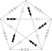
Figure 1: The quiver diagram for the non-supersymmetric freely acting $\mathbb{Z}_{5}$ orbifold.

There are five $SU(3)$ triplets of chiral fermions, $\psi^{i}_{k,k+1}$, on the boundary of the quiver as well as five $SU(3)$ singlet chiral fermions $\chi_{k,k+2}$ and five complex $SU(3)$ triplets, $\Phi^{i}_{k,k+2}$ corresponding to the edges of the star.

The explicit form of the $SU(3)$ octets (74) is

$$O_{n}^{\langle i{\bar{\jmath}}\rangle}\equiv\mbox{Tr}(g^{n}\phi^{i}\phi^{\bar{\jmath}})-\frac{1}{3}\eta^{i{\bar{\jmath}}}\mbox{Tr}(g^{n}\phi^{k}\phi^{\bar{k}})=\sum_{k=1}^{5}\left(\Phi^{i}_{k,k+2}\Phi^{{\bar{\jmath}}}_{k+2,k}-{1\over 3}\eta^{i{\bar{\jmath}}}\Phi^{l}_{k,k+2}\Phi^{\bar{l}}_{k+2,k}\right)e^{in\alpha(k-1)}~{}~{},$$ (75)

where $n$ assumes values $-2,-1,0,1,2$. The deformation of the tree level Lagrangian is:

$$\delta_{\rm 2~{}trace}{\cal L}=f_{{\bf 8},1}O_{1}^{\langle i{{\bar{\jmath}}}\rangle}O_{-1}^{\langle j{\bar{\imath}}\rangle}+f_{{\bf 8},2}O_{2}^{\langle i{\bar{\jmath}}\rangle}O_{-2}^{\langle j{{\bar{\imath}}}\rangle}+f_{{\bf 1},1}O_{1}O_{-1}+f_{{\bf 1},2}O_{2}O_{-2}$$ (76)

Putting this together with the general expression in section 3 yields the beta functions for the four twisted couplings $f$:

$$\beta_{{\bf 8},1} = \frac{1}{160\pi^{2}}\left[\left(f_{{\bf 8},1}+2\left(5+\sqrt{5}\right)\right)^{2}-40(\sqrt{5}+1){\lambda^{2}}\right]$$ (77)

$$\beta_{{\bf 8},2} = \frac{1}{160\pi^{2}}\left[\left(f_{{\bf 8},2}+2(5-\sqrt{5})\right)^{2}+40(\sqrt{5}-1){\lambda^{2}}\right]$$ (78)

$$\beta_{{\bf 1},1} = \frac{3}{160\pi^{2}}\left[\left(f_{{\bf 1},1}+\frac{1}{3}\left(19-\sqrt{5}\right)\right)^{2}-\frac{16}{9}(7\sqrt{5}+1){\lambda^{2}}\right]$$ (79)

$$\beta_{{\bf 1},2} = \frac{3}{160\pi^{2}}\left[\left(f_{{\bf 1},2}+\frac{1}{3}\left(19+\sqrt{5}\right)\right)^{2}+\frac{16}{9}(7\sqrt{5}-1){\lambda^{2}}\right]$$ (80)

We observe that the beta functions for the singly-charged octet and singlet operators have nontrivial zeroes at real values of the coupling, while the coupling constants of the doubly-charged operators do not.

5.2 The ${\cal N}=1$ supersymmetric $\mathbb{Z}_{3}$ orbifold

The smallest quiver gauge theory in the class (65) is the $\mathbb{Z}_{3}$, which has $\omega_{3}=e^{2\pi i/3}$. In this case, one of the eigenvalues of $r(g)$ equals $1$, hence the orbifold preserves ${\cal N}=1$ supersymmetry [6, 7]. One finds $U(N)^{3}/U(1)$ supersymmetric gauge theory coupled to three bifundamental chiral superfields on each edge of the triangular quiver diagram. While outside the main goal of this section, the analysis of this theory exposes important subtleties.

The single-trace operators quadratic in the scalar fields again break up into octets

$$O_{n}^{\langle i{\bar{\jmath}}\rangle}=\sum_{k=1}^{3}\left(\Phi^{i}_{k,k-1}\Phi^{{\bar{\jmath}}}_{k-1,k}-{1\over 3}\eta^{i{\bar{\jmath}}}\Phi^{l}_{k,k-1}\Phi^{\bar{l}}_{k-1,k}\right)e^{in\alpha(k-1)}~{}~{},$$ (81)

and singlets

$$O_{n}=\sum_{k=1}^{3}\Phi^{i}_{k,k-1}\Phi^{{\bar{\imath}}}_{k-1,k}e^{in\alpha(k-1)}~{}~{},$$ (82)

where $n$ assumes values $-1,0,1$.

Specifying the result (126) of Appendix B to this $\mathbb{Z}_{3}$ case, we find that the $O(\lambda^{2})$ source term in the octet beta function $\beta_{{\bf 8},1}$ vanishes. Therefore, the operator $O_{1}^{\langle i{{\bar{\imath}}}\rangle}O_{-1}^{\langle j{{\bar{\imath}}}\rangle}$ is not generated along the fixed line emanating from the origin of the coupling constant space. However, (126) does give an $O(\lambda^{2})$ source in the beta function for the singlet operator $O_{1}O_{-1}$. To explain the physical meaning of this, we recall that the standard orbifold projection method yields $U(N)^{k}/U(1)$ theories which contain non-conformal $U(1)$ factors with abelian charges $e$ set equal to the $SU(N)$ charges $g_{\scriptscriptstyle YM}$. In [29] this choice of parameters was called the “natural line.” On this line the theory cannot be conformal because $\beta_{e}$ is positive. For example in the supersymmetric $\mathbb{Z}_{3}$ case,

$$\beta_{e}={3\over 16\pi^{2}}e^{3}N\ .$$ (83)

The contributions to the potential from the D-terms of the $U(1)$ factors give

$${e^{2}\over 2}\left(|\Phi^{i}_{1,2}|^{2}-|\Phi^{i}_{1,3}|^{2}\right)^{2}+{e^{2}\over 2}\left(|\Phi^{i}_{1,2}|^{2}-|\Phi^{i}_{2,3}|^{2}\right)^{2}+{e^{2}\over 2}\left(|\Phi^{i}_{2,3}|^{2}-|\Phi^{i}_{1,3}|^{2}\right)^{2}=e^{2}O_{1}O_{-1}$$ (84)

Thus, on the natural line the singlet double-trace operator is automatically present in the tree-level action, with coefficient $e^{2}$. The flow of the abelian charge $e$ (83) then explains why there must be a beta function generated for the singlet double-trace operator. The RG flow should take the theory from the natural line $e=g_{\scriptscriptstyle YM}$ to the actual fixed line where $e=0$ and the $U(1)$ factors decouple. By supersymmetry we then expect (although have not checked in detail) that on the fixed line no double trace operator $O_{1}O_{-1}$ is generated.

In fact, the concern about the role of the $U(1)$ factors in orbifold calculations for bifundamental scalars is general and applies to both supersymmetric and non-supersymmetric examples. The simple method of orbifold projection in field theory [9] is very efficient in producing results on the natural line, and we adopt it in our paper. But to understand the fixed line one needs more complicated calculations where the $U(1)$ factors are decoupled and we have a $SU(N)^{k}$ theory. We note, however, that the $U(1)$’s affect only the double-trace operators made out of $SU(3)$ singlets. Thus, we can certainly take our results for $SU(3)$ adjoint beta functions $\beta_{{\bf 8},n}$ as applicable to the $SU(N)^{k}$ theory, and not just to the $U(N)^{k}/U(1)$ theory.

5.3 $\mathbb{Z}_{6}$

The field content is quite similar to the one in the $\mathbb{Z}_{5}$ theory, so we will not describe it again. The quiver summarizing it is shown in figure 2.

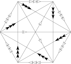
Figure 2: The quiver diagram for the non-supersymmetric freely acting $\mathbb{Z}_{6}$ orbifold.

It turns out that in this case not all octet operators are generated at one-loop level: $O_{2}^{\langle i{{\bar{\jmath}}}\rangle}O_{-2}^{\langle j{{\bar{\imath}}}\rangle}$ is not generated. This can be traced to the fact that the orbifold action has a $\mathbb{Z}_{3}$ subgroup $\{1,g^{2},g^{4}\}$ which preserves the ${\cal N}=1$ supersymmetry. Therefore, we may choose to deform the tree-level action only with

$$\delta_{\rm 2~{}trace}S = f_{{\bf 8},1}O_{1}^{\langle i{{\bar{\jmath}}}\rangle}O_{-1}^{\langle j{{\bar{\imath}}}\rangle}+\frac{1}{2}f_{{\bf 8},3}O_{3}^{\langle i{{\bar{\jmath}}}\rangle}O_{-3}^{\langle j{{\bar{\imath}}}\rangle}+f_{{\bf 1},1}O_{1}O_{-1}+f_{{\bf 1},2}O_{2}O_{-2}+\frac{1}{2}f_{{\bf 1},3}O_{3}O_{-3}$$ (85)

$$\beta_{{\bf 8},1} = \frac{1}{192\pi^{2}}\left[(f_{{\bf 8},1}+12\lambda)^{2}-80{\lambda^{2}}\right]$$ (86)

$$\beta_{{\bf 8},3} = \frac{1}{192\pi^{2}}\left[f_{{\bf 8},3}^{2}+64{\lambda^{2}}\right]$$ (87)

$$\beta_{{\bf 1},1} = \frac{1}{64\pi^{2}}\left[(f_{{\bf 1},1}+6\lambda)^{2}-\frac{320}{9}\lambda^{2}\right]$$ (88)

$$\beta_{{\bf 1},2} = \frac{1}{64\pi^{2}}\left[(f_{{\bf 1},2}+6\lambda)^{2}\right]$$ (89)

$$\beta_{{\bf 1},3} = \frac{1}{64\pi^{2}}\left[(f_{{\bf 1},3}+4\lambda)^{2}+\frac{112}{9}\lambda^{2}\right]$$ (90)

Thus, we see that only the beta functions for the highest charge operators do not posses a nontrivial zero at real values of the double-trace coupling constant.

As we will see however in the next subsection, the fact that only a small number of couplings have positive beta functions is nongeneric within the class of orbifolds considered here; roughly speaking, about one quarter of all double-trace operators have this unfortunate property.

5.4 $\mathbb{Z}_{k}$ with $SU(3)$ symmetry

It is relatively easy to specialize the results obtained in section 3 to the case of $\mathbb{Z}_{k}$ with $SU(3)$ symmetry and we spell this out in the Appendix C. The point worth emphasizing here is that, similarly to the $\mathbb{Z}_{5}$ and $\mathbb{Z}_{6}$ examples, the double-trace tree-level terms are:

$$\delta S^{\rm tree}_{\rm 2~{}trace} = \frac{1}{2}\sum_{n=1}^{k-1}\,f_{{\bf 8},n}O_{n}^{\langle i{\bar{\jmath}}\rangle}O_{-n}^{\langle j{\bar{\imath}}\rangle}+\frac{1}{2}\sum_{n=1}^{k-1}\,f_{{\bf 1},n}O_{n}O_{-n}$$ (91)

with the symmetry

$$f_{{\bf 8},n}=f_{{\bf 8},k-n}~{}~{}~{}~{}~{}~{}~{}~{}f_{{\bf 1},n}=f_{{\bf 1},k-n}$$ (92)

This choice of coefficients leads to unified expressions for the beta functions for the couplings $f_{{\bf 1},n}$ and $f_{{\bf 8},n}$ for all values of the charge. The calculations described in the Appendix C leads to the following beta functions:

$$\beta_{8,n} = \frac{1}{32\pi^{2}k}\left[(f_{8,n}+2\delta_{8,n})^{2}-256\lambda^{2}\left(3+4\cos(n\alpha_{k})\right)\sin^{4}\left({\textstyle{\frac{1}{2}}}n\alpha_{k}\right)\right]$$ (93)

$$\beta_{1,n} = \frac{3}{32\pi^{2}k}\left[\left(f_{1,n}+\frac{2}{3}\delta_{1,n}\right)^{2}-\frac{64}{9}\lambda^{2}\left(1+2\cos(n\alpha_{k})\right)\left(4-2\cos(n\alpha_{k})+\cos(2n\alpha_{k})\right)\right]$$

     

The figures above represent plots of the discriminants of the equations imposing the vanishing of the octet and singlet beta functions, respectively. The circular dots and upright triangles correspond to the $\mathbb{Z}_{5}$ and $\mathbb{Z}_{6}$ examples discussed in the beginning of this section.

From (93) we see that the charge $m$ operators appearing in the $\mathbb{Z}_{2m}$ theory are special in that, up to the factor of $1/|\Gamma|$, the beta functions for their coefficients are equal. This is the manifestation of the fact emphasized in the beginning that, in a sense, this operator can be thought of as being inherited from a $\mathbb{Z}_{2}$-orbifold field theory analogous to the one discussed in section 4.1.

Another important point is that all orbifold field theories of the type discussed in this section posses at least one deformation made out of $SU(3)$ adjoints which spoils conformal symmetry. Indeed, the beta function of all such operators with

$$-1\leq\cos\left(2\pi{{\frac{n}{k}}}\right)<-\frac{3}{4}$$ (94)

has a negative discriminant and hence no real solutions for the coupling constant. Such operators are not affected by the contributions of the twisted $U(1)$’s, which need to be removed from the orbifold theory because they become free in the IR. Therefore, even without performing the more laborious calculations which separate out the $U(1)$’s, we conclude that there is no fixed line passing through the origin in the non-supersymmetric theories with the $SU(3)$ symmetry.

6 Discussion

In this paper we searched for perturbative fixed lines in $d=4$ non-supersymmetric large $N$ orbifold gauge theories. This required a careful calculation of the one-loop beta-functions for double-trace operators made of scalar fields. In the examples we considered, both freely acting and not, we found that there are no fixed lines passing through the origin in the coupling constant space $(f^{i},\lambda)$. We hope to return to perturbative analysis of more general gauge theories in the future.

Let us consider how our one-loop results may be modified by higher order corrections. The two-loop correction to $\beta_{f}$ has the general structure

$$\delta\beta_{f}=wf^{3}+v_{1}\lambda f^{2}+2\gamma_{1}f\lambda^{2}+a_{1}\lambda^{3}\ .$$ (95)

For example, the third term arises through a two-loop correction to the anomalous dimension of $O$, $\gamma_{1}\lambda^{2}$. For $f$ of order $\lambda$ these terms are of order $\lambda^{3}$ and are suppressed at weak coupling compared to the one-loop contributions. Thus, the two-loop correction is small near the origin of the coupling constant space. If a real solution $f=a\lambda$ exists at one-loop order then it should be possible to correct it, $f=a\lambda+b\lambda^{2}$, so that the two-loop solution exists to order $\lambda^{3}$. Iterating this procedure order by order, we would conclude that if a real one-loop solution exists then there is indeed a fixed line passing through the origin of the coupling constant space.

In cases where one-loop beta function equation has no real solutions, we cannot rule out a possibility that there is a fixed line passing away from the origin, although it is difficult to study perturbatively. Another possibility is that there is a line of fixed points which terminates at some critical value $\lambda_{c}$ without reaching the weak coupling region. Indeed, for freely acting orbifolds, such as the $SU(3)$ symmetric family we considered, there is evidence from AdS/CFT for a fixed line at very large values of $\lambda$ where there are no tachyons in the twisted sector. We will comment on a possible mechanism for a phase transition at $\lambda_{c}$ later in this section. In any case, our perturbative calculation shows that this fixed line cannot pass through the origin of the coupling constant space, but it would be interesting to examine more general freely acting orbifolds.

For instance, certain product group orbifolds, such as $\mathbb{Z}_{m}\times\mathbb{Z}_{n}$ orbifolds, appear promising in this direction. In our discussion of the $\mathbb{Z}_{n}$ orbifolds with $SU(3)$ symmetry we saw that, in some cases, the beta functions without fixed points are associated with the operators charged under some non-freely acting subgroup of the full orbifold group. Thus, a step toward finding a non-supersymmetric conformal orbifold in the large $N$ limit could be ensuring that such operators are not generated. For a product group orbifold we may choose that each of the individual factors acts in a supersymmetric way, but preserving different subalgebras of the ${\cal N}=4$ supersymmetry algebra. One example is the freely acting $\mathbb{Z}_{3}\times\mathbb{Z}_{3}$ orbifold where the first $\mathbb{Z}_{3}$ is generated by $r=(\omega_{3},\omega_{3},\omega_{3},1)$ and the second by $r^{\prime}=(1,\omega_{3},\omega_{3},\omega_{3})$. Thus, each $\mathbb{Z}_{3}$ preserves ${\cal N}=1$ supersymmetry by itself, but the combined orbifold breaks all supersymmetry. In this class of orbifolds, some double-trace operators are not generated due to the supersymmetry of the individual factors. It would be very interesting to examine all double-trace beta functions, after eliminating by hand the twisted $U(1)$ factors.

Finally, we suggest a relation of our calculations to closed string tachyon condensation. In freely acting orbifolds of $AdS_{5}\times S^{5}$, all twisted sector tachyons are lifted at large $\lambda$ because the twisted strings are highly stretched. Schematically, the effective potential for such a charged field in $AdS_{5}$ has the form

$$V(T)={1\over 2}m^{2}(\lambda)T^{*}T+{c_{4}\over 4}(T^{*}T)^{2}+\ldots\ ,$$ (96)

where at strong coupling $m^{2}(\lambda)\sim\lambda/\alpha^{\prime}$. In [30, 31] a similar effective potential was studied in a simpler case of the Rohm compactification, where $T$ corresponds to a string winding around a circle. In that case $c_{4}$ was found to be positive; we will assume that it is positive also in (96). Since the twisted sector strings have negative zero-point energy, $m^{2}(\lambda)$ is expected to become negative for $\lambda<\lambda_{c}$, where $\lambda_{c}$ is of order $1$. This may cause a transition to a phase where $T$ has an expectation value (however, the local maximum of the potential at $T=0$ is stable if $m^{2}$ is not too negative, due to the well-known Breitenlohner-Freedman bound in AdS space [32]). What would be a manifestation of the tachyon condensation in the dual gauge theory? The logarithmic running of double-trace operators $O_{n}O_{-n}$ in the gauge theory is expected to lead to development of expectation values for twisted operators $O_{n}$ through the Coleman-Weinberg mechanism. This breaking of the quantum symmetry $\Gamma$ has been proposed [13] as the gauge theory dual of tachyon condensation. We believe that this mechanism is applicable to both non-freely acting and freely acting orbifolds. Through an explicit gauge theory calculation we find that at weak coupling all possible such trace-squared operators typically get induced. But the arguments based on the AdS/CFT correspondence suggest that, as $\lambda$ is increased, the gauge theory should make a transition to a phase with restored symmetry, i.e. with no running of double-trace operators. This can happen if for sufficiently large ‘t Hooft coupling $\lambda$ all the double trace beta functions acquire real zeros.

If this scenario holds, then for sufficiently large $\lambda$ the perturbative expansion probably breaks down, and the theory enters a different phase which is dual to string theory on $AdS_{5}\times S^{5}/|\Gamma|$ with radius larger than critical. In large-$N$ theories this is a common situation since summation of planar graphs typically has a finite radius of convergence. It is tempting to speculate that this kind of large-$N$ phase transition in non-supersymmetric freely acting orbifold gauge theories corresponds to symmetry restoration.

As we emphasized throughout the paper, there are two possibilities for the behavior of the theory at very weak coupling. The first possibility is that some of the $a^{i}_{\pm}$ are complex. Then for physical (real) values of double-trace couplings, they do not possess fixed points in the perturbative regime and flow away from it, leading to runaway behavior in the large $N$ limit. The examples we have considered so far exhibit only this effect, which is a rather uncontrollable tachyon condensation. The second possibility is that all $a^{i}_{\pm}$ are real. Then all double-trace couplings flow to zeros of their beta functions, and we have a fixed line passing through the origin of the coupling constant space. In such a theory there does not seem to be a phase transition that could correspond to tachyon condensation. It remains to be seen whether there exist examples of such theories.

Appendix A Orbifold traces of Dirac matrices

As we have seen in section 3, the contribution of the fermions to the effective action depends on the tensor

$$\mbox{Tr}[\gamma^{I}\gamma^{J}\gamma^{K}\gamma^{L}r_{g}]~{}~{},$$ (97)

where $\gamma$ are six-dimensional chiral (i.e. $4\times 4$) Dirac matrices and $r_{g}$ is the realization of the orbifold group element $g$ on the fundamental representation of $SU(4)$.

This trace can be computed for a general $r_{g}$-matrix. The idea is to use the explicit form of the Dirac matrices, which can be inferred from the fact that they realize the map between the ${\bf 6}$ of $SO(6)$ and $SU(4)$. This map naturally splits the $SO(6)$ vector indices into complex three-dimensional indices: $I=(i,\,{{\bar{\imath}}})$. Also, this map singles out the fourth component of the fundamental representation of $SU(4)$ and splits the four-dimensional index as $\alpha=(i,4)$.

The nonvanishing traces are:

$$\frac{1}{4}Tr[\gamma^{{\bar{\imath}}}\gamma^{{\bar{\jmath}}}\gamma^{k}\gamma^{l}r_{g}] = \epsilon^{klx}r_{x}{}^{y}\epsilon_{yji}$$ (98)

$$\frac{1}{4}Tr[\gamma^{i}\gamma^{{\bar{\jmath}}}\gamma^{k}\gamma^{\bar{l}}r_{g}] = (\delta^{i}_{j}\delta^{k}_{l}r_{4}{}^{4}+\delta^{k}_{j}r_{l}{}^{i})$$ (99)

$$\frac{1}{4}Tr[\gamma^{i}\gamma^{{\bar{\jmath}}}\gamma^{\bar{k}}\gamma^{l}r_{g}] = (r_{j}{}^{i}\delta_{k}^{l}-r_{k}{}^{i}\delta_{j}^{l})$$ (100)

$$\frac{1}{4}Tr[\gamma^{{\bar{\imath}}}\gamma^{j}\gamma^{k}\gamma^{\bar{l}}r_{g}] = (r_{l}{}^{k}\delta_{i}^{j}-r_{l}{}^{j}\delta_{i}^{k})$$ (101)

$$\frac{1}{4}Tr[\gamma^{{\bar{\imath}}}\gamma^{j}\gamma^{\bar{k}}\gamma^{l}r_{g}] = (r_{x}{}^{x}\delta_{i}^{j}\delta_{k}^{l}+\delta_{i}^{l}r_{k}{}^{j}-\delta_{k}^{l}r_{i}{}^{j}-\delta_{i}^{j}r_{k}{}^{l})$$ (102)

$$\frac{1}{4}Tr[\gamma^{i}\gamma^{j}\gamma^{\bar{k}}\gamma^{\bar{l}}r_{g}] = r_{4}{}^{4}(\delta_{l}^{i}\delta_{k}^{j}-\delta_{k}^{i}\delta_{l}^{j})$$ (103)

$$\frac{1}{4}Tr[\gamma^{i}\gamma^{{\bar{\jmath}}}\gamma^{k}\gamma^{l}r_{g}] = \delta_{j}^{i}\epsilon^{lkx}r_{x}{}^{4}$$ (104)

$$\frac{1}{4}Tr[\gamma^{{\bar{\imath}}}\gamma^{j}\gamma^{\bar{k}}\gamma^{\bar{l}}r_{g}] = (r_{4}{}^{y}\delta_{i}^{j}-r_{4}{}^{j}\delta_{i}^{y})\epsilon_{ylk}$$ (105)

$$\frac{1}{4}Tr[\gamma^{i}\gamma^{j}\gamma^{\bar{k}}\gamma^{l}r_{g}] = (\delta_{x}^{i}\delta_{k}^{j}-\delta_{x}^{j}\delta_{k}^{i})\epsilon^{lxy}r_{y}{}^{4}$$ (106)

$$\frac{1}{4}Tr[\gamma^{{\bar{\imath}}}\gamma^{{\bar{\jmath}}}\gamma^{k}\gamma^{\bar{l}}r_{g}] = \delta^{k}_{l}r_{4}{}^{y}\epsilon_{yij}$$ (107)

$$\frac{1}{4}Tr[\gamma^{i}\gamma^{j}\gamma^{k}\gamma^{\bar{l}}r_{g}] = \epsilon^{ikj}r_{l}{}^{4}$$ (108)

$$\frac{1}{4}Tr[\gamma^{i}\gamma^{{\bar{\jmath}}}\gamma^{\bar{k}}\gamma^{\bar{l}}r_{g}] = r_{4}{}^{i}\epsilon_{jkl}$$ (109)

For abelian orbifolds one may diagonalize simultaneously all the group generators and thus one may pick $r_{g}$ to be diagonal. Then, the expressions above simplify considerably, in part due to the vanishing of the last six lines.

Appendix B Renormalization of a single-trace operator

The action of the 1-loop dilatation operator on long twisted operators in the SU(2) sector was discussed in [35]. However, this discussion does not directly apply to operators of dimension 2, because in this case there exist additional planar diagrams. Furthermore, we are interested in more general operators than those present in the $SU(2)$ sector.

The most general single-trace dimension 2 twisted operator is

$$\mbox{Tr}(g\phi^{I}\phi^{J})~{}~{}.$$ (110)

The action of the dilatation operator is easy to find:

$$\Delta(\mbox{Tr}(g\phi^{I}\phi^{J}))={\lambda\over 16\pi^{2}\,|\Gamma|}\Big{[}\mbox{Tr}(g\phi^{I}\phi^{J})-$$ (111)

$$-{1\over|\Gamma|}\sum_{{\tilde{g}}_{1},{\tilde{g}}_{2}\in\Gamma}(R_{{\tilde{g}}_{1}})^{I^{\prime}I}(R_{{\tilde{g}}_{2}})^{J^{\prime}J}\left(\delta^{KJ^{\prime}}\delta^{LI^{\prime}}-{1\over 2}\delta^{KI^{\prime}}\delta^{LJ^{\prime}}-{1\over 2}\delta^{I^{\prime}J^{\prime}}\delta^{KL}\right)\times$$ (112)

$$~{}~{}~{}~{}~{}~{}~{}~{}~{}~{}~{}~{}~{}~{}~{}~{}~{}~{}~{}~{}~{}~{}~{}~{}~{}~{}~{}~{}~{}~{}~{}~{}\times\left(\mbox{Tr}(g{\tilde{g}}_{1}\phi^{L}\phi^{K}{\tilde{g}}_{1}^{\dagger})\delta_{{\tilde{g}}_{2}=g{\tilde{g}}_{1}}+\mbox{Tr}(g{\tilde{g}}_{2}\phi^{K}\phi^{L}{\tilde{g}}_{2}^{\dagger})\delta_{{\tilde{g}}_{1}={\tilde{g}}_{2}}\right)\Big{]}$$ (113)

This expression can be organized in various ways, each form emphasizing different aspects of $\Delta$. For example,

$$\Delta(\mbox{Tr}(g\phi^{I}\phi^{J}))={\lambda\over 8\pi^{2}|\Gamma|}\left[\mbox{Tr}(g[\phi^{I},g]g^{\dagger}\phi^{J})+\mbox{Tr}(g[\phi^{I},\phi^{J}])+{1\over 2}(\delta^{IJ}+R_{g}{}^{J}{}^{I})\sum_{K}\mbox{Tr}(g\phi^{K}\phi^{K})\right]$$ (114)

implies that traceless $\Gamma$-invariant bilinears have zero anomalous dimension at one loop.

Alternatively, (113) can be cast in a form very similar to the dilatation operator in the parent theory

$$\Delta\left(\mbox{Tr}(g\phi^{I}\phi^{J})\right) = {\lambda\over 16\pi^{2}|\Gamma|}\bigg{[}4\mbox{Tr}(g\phi^{I}\phi^{J})+\left(\delta^{IJ}+R_{g}^{JI}\right)\sum_{K}\mbox{Tr}(g\phi^{K}\phi^{K})$$ (115)

$$- 2\left(\mbox{Tr}(g\phi^{I}\phi^{K})\left(R_{g}\right){}^{KJ}+\left(R_{g}^{-1}\right){}^{IK}\mbox{Tr}(g\phi^{K}\phi^{J})\right)\bigg{]}~{}~{},$$ (116)

which makes it easy to compute the anomalous dimensions in cases in which $R_{g}$ is diagonal.

Appendix C $\mathbb{Z}_{k}$ with $SU(3)$ symmetry

C.1 Anomalous dimensions

It is easy to see from (116) that the “off-diagonal operators” – $\mbox{Tr}(g^{n}\,\phi^{i}\phi^{{\bar{\jmath}}})$ with $i\neq j$ – have definite anomalous dimensions:

$$\Delta\mbox{Tr}(g^{n}\,\phi^{i}\phi^{{\bar{\jmath}}})\Big{|}_{i\neq j}\!\!=\frac{\lambda}{16\pi^{2}k}\left[\,8\sin^{2}(n\alpha_{k})\,\mbox{Tr}(g^{n}\,\phi^{i}\phi^{{\bar{\jmath}}})\Big{|}_{i\neq j}\right]\ .$$ (117)

The diagonal operators however – $\mbox{Tr}(g^{n}\phi^{i}\phi^{{\bar{\imath}}})$ – mix under RG flow. Their mixing matrix is

$$\Delta{\cal O}_{n}=\frac{\lambda}{16\pi^{2}k}\begin{pmatrix}4\sin^{2}(n\alpha_{k})+4&4\cos^{2}(n\alpha_{k})&4\cos^{2}(n\alpha_{k})\cr 4\cos^{2}(n\alpha_{k})&4\sin^{2}(n\alpha_{k})+4&4\cos^{2}(n\alpha_{k})\cr 4\cos^{2}(n\alpha_{k})&4\cos^{2}(n\alpha_{k})&4\sin^{2}(n\alpha_{k})+4\end{pmatrix}{\cal O}_{n}$$ (118)

where

$${\cal O}_{n}=\begin{pmatrix}\mbox{Tr}(g^{n}\phi^{1}\phi^{\bar{1}})\cr\mbox{Tr}(g^{n}\phi^{2}\phi^{\bar{2}})\cr\mbox{Tr}(g^{n}\phi^{3}\phi^{\bar{3}})\end{pmatrix}$$ (119)

Its diagonal form is:

$$\Delta{\widetilde{\cal O}}_{n}=\frac{\lambda}{16\pi^{2}k}\begin{pmatrix}2\left(5+\cos(2n\alpha_{k})\right)&0&0\cr 0&8\sin^{2}(n\alpha_{k})&0\cr 0&0&8\sin^{2}(n\alpha_{k})\end{pmatrix}{\widetilde{\cal O}}_{n}$$ (120)

For $n=0$ we recover the well-known value of the 1-loop anomalous dimension of the Konishi operator. Collecting everything we find the operators and dimensions quoted in (74).

C.2 Effective action

The bosonic and ghost loop contribution is

$$\delta S^{\rm 1~{}loop|2~{}tr}_{\rm Bose,\,ghost} = -\frac{{\rm Div}}{2\,k}\sum_{n=0}^{k-1}\Big{\{}\hphantom{-}8\big{(}\cos^{2}(n\alpha_{k})\left(3\cos(2n\alpha_{k})+1\right)+2\sin^{2}(2n\alpha_{k})\big{)}O_{n}O_{-n}$$ (122)

$$~{}~{}~{}~{}~{}~{}~{}~{}~{}~{}~{}~{}~{}~{}+8\big{(}2+\cos(2n\alpha_{k})+\cos(4n\alpha_{k})\big{)}O^{i{\bar{\jmath}}}_{n}O^{j{\bar{\imath}}}_{-n}~{}~{}~{}~{}\Big{\}}$$

The fermionic contribution is

$$\delta S^{\rm 1~{}loop|2~{}tr}_{\rm Fermi} = \frac{{\rm Div}}{2\,k}\sum_{n=0}^{k-1}\,\Big{\{}\hphantom{-}8\big{(}4\cos^{3}(n\alpha_{k})+\cos(n\alpha_{k})-\cos(3n\alpha_{k})\big{)}O_{n}O_{-n}$$ (124)

$$~{}~{}~{}~{}~{}~{}~{}~{}~{}~{}~{}~{}~{}+8\big{(}4\cos^{3}(n\alpha_{k})-\cos(n\alpha_{k})+\cos(3n\alpha_{k})\big{)}O_{n}^{i{{\bar{\jmath}}}}O_{-n}^{j{\bar{\imath}}}~{}~{}~{}~{}\Big{\}}$$

Adding the equations (124) and (122) and expressing the result in terms of operators with definite 1-loop scaling dimension leads to:

$$\delta S^{\rm 1~{}loop|2~{}tr}_{\rm\scriptscriptstyle Bose,\,ghost,Fermi} = -\frac{{\rm Div}}{2\,k}\sum_{n=1}^{k-1}\Bigg{[}\hphantom{+}\frac{256}{3}\sin^{8}\left({\textstyle{\frac{1}{2}}}n\alpha_{k}\right)\,O_{n}O_{-n}$$ (126)

$$~{}~{}~{}~{}~{}~{}~{}~{}~{}~{}~{}~{}~{}~{}~{}~{}~{}~{}~{}~{}+64(1+2\cos(n\alpha_{k}))^{2}\sin^{4}\left({\textstyle{\frac{1}{2}}}n\alpha_{k}\,\right)O^{\langle i{\bar{\jmath}}\rangle}_{n}O^{\langle j{\bar{\imath}}\rangle}_{-n}~{}~{}~{}\Bigg{]}$$

We add the following double-trace terms to the tree-level action:

$$\delta S^{\rm tree}_{\rm 2~{}trace} = \frac{1}{2}\sum_{n=1}^{k-1}\,f_{{\bf 8},n}O_{n}^{\langle i{\bar{\jmath}}\rangle}O_{-n}^{\langle j{\bar{\imath}}\rangle}+\frac{1}{2}\sum_{n=1}^{k-1}\,f_{{\bf 1},n}O_{n}O_{-n}$$ (127)

with the symmetry

$$f_{{\bf 8},n}=f_{{\bf 8},k-n}~{}~{}~{}~{}~{}~{}~{}~{}f_{{\bf 1},n}=f_{{\bf 1},k-n}$$ (128)

For each $SU(3)$ structure there are $[k/2]$ independent couplings and hence $[k/2]$ beta functions.

The contribution to the effective action:

$$\delta S^{\rm 1~{}loop|2~{}tr}_{\rm 2~{}trace} = -\frac{{\rm Div}}{2\,k}\Bigg{[}\hphantom{+}\sum_{n=1}^{k-1}\,\frac{f^{2}_{{\bf 8},n}}{4}O_{n}^{\langle i{\bar{\jmath}}\rangle}O_{-n}^{\langle j{\bar{\imath}}\rangle}+\sum_{n=1}^{k-1}\,\frac{3f^{2}_{{\bf 1},n}}{4}O_{n}O_{-n}$$ (130)

$$~{}~{}~{}~{}~{}~{}~{}~{}+\sum_{n=1}^{k-1}\,\delta_{{\bf 8},n}\,f_{{\bf 8},n}O_{n}^{\langle i{\bar{\jmath}}\rangle}O_{-n}^{\langle j{\bar{\imath}}\rangle}+\sum_{n=1}^{k-1}\,\delta_{{\bf 1},n}\,f_{{\bf 1},n}O_{n}O_{-n}\Bigg{]}$$

$$\gamma_{{\bf r},n}=\frac{1}{16\pi^{2}\,k}\,\delta_{{\bf r},n}$$ (131)

are the anomalous dimensions of the operators with representation and charge $({\bf r},n)$.

The beta functions are then given by:

$$\beta_{8,n} = \frac{1}{16\pi^{2}\,k}\left[128(1+2\cos\left(n\alpha_{k}\right))^{2}\sin^{4}\!\left({\textstyle{\frac{1}{2}}}n\alpha_{k}\right)\lambda^{2}+\frac{f_{{\bf 8},n}^{2}}{2}+2\delta_{{\bf 8},n}f_{{\bf 8},n}\right]$$ (132)

$$\beta_{1,n} = \frac{1}{16\pi^{2}\,k}\left[\frac{512}{3}\sin^{8}\!\left({\textstyle{\frac{1}{2}}}n\alpha_{k}\right)\lambda^{2}+\frac{3f_{{\bf 1},n}^{2}}{2}+2\delta_{{\bf 1},n}f_{{\bf 1},n}\right]$$ (133)

It is then a simple exercise to use the anomalous dimensions (74) and obtain the beta functions (93).

Appendix D $\mathbb{Z}_{k}$ with fixed points and $SO(4)$ global symmetry

In this appendix we summarize the effective action of the orbifold field theories with $SO(4)$ global symmetry. They are [24] the gauge theory realizations of the well-known orbifolds $\mathbb{C}^{2}\times\mathbb{C}/\mathbb{Z}_{k}$ with $D3$ branes placed at the tip of the cone (for a recent review see [26]).

D.1 Spectrum

As in the previous case, we choose the standard representation of $\mathbb{Z}_{k}$ on the gauge degrees of freedom. Furthermore, we will choose the following action on the fundamental representation of $SU(4)$ and the vector representation of $SO(6)$:

$$r={\rm diag}(\omega_{k},\omega_{k},\omega_{k}^{-1},\omega_{k}^{-1})$$ (134)

$$R={\rm diag}(1,1,\omega_{k}^{2},1,1,\omega_{k}^{-2})$$ (135)

where the two entries different from unity are the weights of $\phi^{3}$ and $\phi^{\bar{3}}$, respectively.

We will use real indices for the uncharged fields and complex indices for $\phi^{3}$ and $\phi^{\bar{3}}$. Furthermore, the metric on this space of fields is:

$$\eta={\scriptsize{\begin{pmatrix}1&0&0&0&0&0\cr 0&1&0&0&0&0\cr 0&0&1&0&0&0\cr 0&0&0&1&0&0\cr 0&0&0&0&0&1\cr 0&0&0&0&1&0\end{pmatrix}}}$$ (136)

The invariant fields allow the construction of the following operators:

$$O_{n}^{\langle\mu\nu\rangle}=\mbox{Tr}(g^{n}\phi^{\mu}\phi^{\nu})-\frac{1}{4}\delta^{\mu\nu}O_{n}\ ,~{}~{}~{}~{}~{}~{}~{}O_{n}=\sum_{a=1}^{4}\mbox{Tr}(g^{n}\phi^{\kappa}\phi^{\kappa})\ ,~{}~{}~{}~{}~{}~{}~{}A_{n}=\omega_{k}^{n}\mbox{Tr}(g^{n}\phi^{3}\phi^{\bar{3}})\ .$$ (137)

The reason for the apparently strange phase in $A_{n}$ is that with this normalization the entries of the anomalous dimension matrix are real.

D.2 Effective action

The bosonic, ghost and fermionic contribution to the effective action is:

$$\delta S^{\rm\scriptscriptstyle{1~{}loop|2~{}tr}}_{\rm\scriptscriptstyle{b,gh,f}} = -\frac{{\rm Div}}{2\,k}\sum_{n=1}^{k-1}\Bigg{[}\hphantom{+}16\sin^{4}({\textstyle{\frac{1}{2}}}n\alpha_{k})\left(2O_{n}^{\langle\mu\nu\rangle}O_{-n}^{\langle\mu\nu\rangle}+\frac{3}{2}O_{n}O_{-n}\right)$$

$$~{}~{}~{}~{}~{}~{}~{}~{}~{}~{}~{}~{}~{}~{}+32\left(7+4\cos(n\alpha_{k})+\cos(2n\alpha_{k})\right)\sin^{4}\left({\textstyle{\frac{1}{2}}}n\alpha_{k}\right)A_{n}A_{-n}$$

$$~{}~{}~{}~{}~{}~{}~{}~{}~{}~{}~{}~{}~{}~{}-32(2+\cos(n\alpha_{k}))\sin^{4}\left({\textstyle{\frac{1}{2}}}n\alpha_{k}\right)\left(O_{n}A_{-n}+O_{-n}A_{n}\right)~{}~{}~{}~{}~{}\Bigg{]}$$

$$\delta_{\rm{\scriptscriptstyle 2\,tr}}S=\frac{1}{2}\sum_{n=1}^{k-1}\,f_{{\bf 9},n}O_{n}^{\langle\mu\nu\rangle}O_{-n}^{\langle\mu\nu\rangle}+\frac{1}{2}\sum_{n=1}^{k-1}\,f_{{\bf 1},n}O_{n}O_{-n}+\frac{1}{2}\sum_{n=1}^{k-1}\,f_{(3),n}A_{n}A_{-n}+\sum_{n=1}^{k-1}\,\,f_{n}\,O_{n}A_{-n}$$ (140)

with constraints similar to those discussed before:

$$f_{{\bf 9},n}=f_{{\bf 9},k-n}~{}~{}~{}~{}f_{{\bf 1},n}=f_{{\bf 1},k-n}~{}~{}~{}~{}f_{(3),n}=f_{(3),k-n}~{}~{}~{}~{}~{}~{}~{}~{}f_{n}=f_{k-n}$$ (141)

where the last constraint ensures that the deformation of the tree level action is real.

$$\delta S^{\rm 1~{}loop|2~{}tr}_{\rm 2~{}trace} = -\frac{{\rm Div}}{2k}\Bigg{\{}\hphantom{+}\sum_{n=1}^{k-1}\,\frac{f^{2}_{{\bf 9},n}}{2}O_{n}^{\langle\mu\nu\rangle}O_{-n}^{\langle\mu\nu\rangle}+\sum_{n=1}^{k-1}\,\left[2{f^{2}_{{\bf 1},n}}+\frac{1}{4}f_{n}f_{k-n}\right]O_{n}O_{-n}$$ (143)

$$~{}~{}~{}~{}~{}~{}~{}~{}~{}~{}+\sum_{n=1}^{k-1}\,\left[\frac{f^{2}_{(3),n}}{4}+2f_{n}f_{k-n}\right]A_{n}A_{-n}+2\left[2f_{{\bf 1},n}f_{n}+\frac{1}{4}f_{(3),n}f_{n}\right]\,O_{n}A_{-n}$$

$$+ \sum_{n=1}^{k-1}\,\left[f_{{\bf 1},n}\left[\delta_{n}^{OO}O_{n}+\delta_{n}^{OA}A_{n}\right]O_{-n}+f_{(3),n}\left[\delta_{n}^{AO}O_{n}+\delta_{n}^{AA}A_{n}\right]A_{-n}\right]$$ (144)

$$+ \sum_{n=1}^{k-1}\,\,f_{n}\,\left[\left[\delta_{n}^{OO}O_{n}+\delta_{n}^{OA}A_{n}\right]A_{-n}+O_{n}\left[\delta_{-n}^{AO}O_{-n}+\delta_{-n}^{AA}A_{-n}\right]\right]~{}~{}~{}\Bigg{\}}$$ (145)

where the anomalous dimension matrix is:

$$\Delta\begin{pmatrix}O_{n}\cr A_{n}\end{pmatrix}=\frac{1}{16\pi^{2}k}\delta\begin{pmatrix}O_{n}\cr A_{n}\end{pmatrix}=\frac{\lambda}{16\pi^{2}k}\begin{pmatrix}8&16\cos(n\alpha_{k})\cr 2\cos(n\alpha_{k})&4\left(1+\sin^{2}(n\alpha_{4})\right)\end{pmatrix}\begin{pmatrix}O_{n}\cr A_{n}\end{pmatrix}$$ (146)

To extract the beta functions we add (D.2) and (145) while properly keeping track of the charges or operators to eliminate the doubling introduced to make the expressions uniform. It is clear that $\beta_{{\bf 9},n}$ do not have any real zeros, since the corresponding operators have no one-loop anomalous dimensions. This agrees with our general findings for non-freely acting orbifolds in section 4.3.

References

• [1] J. M. Maldacena, “The large N limit of superconformal field theories and supergravity,” Adv. Theor. Math. Phys.  2, 231 (1998) [Int. J. Theor. Phys.  38, 1113 (1999)] [arXiv:hep-th/9711200].
• [2] S. S. Gubser, I. R. Klebanov and A. M. Polyakov, “Gauge theory correlators from non-critical string theory,” Phys. Lett. B 428, 105 (1998) [arXiv:hep-th/9802109].
• [3] E. Witten, “Anti-de Sitter space and holography,” Adv. Theor. Math. Phys.  2, 253 (1998) [arXiv:hep-th/9802150].
• [4] O. Aharony, S. S. Gubser, J. M. Maldacena, H. Ooguri and Y. Oz, “Large N field theories, string theory and gravity,” Phys. Rept.  323, 183 (2000) [arXiv:hep-th/9905111].
• [5] I. R. Klebanov, “TASI lectures: Introduction to the AdS/CFT correspondence,” arXiv:hep-th/0009139.
• [6] S. Kachru and E. Silverstein, “4d conformal theories and strings on orbifolds,” Phys. Rev. Lett.  80, 4855 (1998) [arXiv:hep-th/9802183].
• [7] A. E. Lawrence, N. Nekrasov and C. Vafa, “On conformal field theories in four dimensions,” Nucl. Phys. B 533, 199 (1998) [arXiv:hep-th/9803015].
• [8] M. Bershadsky, Z. Kakushadze and C. Vafa, “String expansion as large N expansion of gauge theories,” Nucl. Phys. B 523, 59 (1998) [arXiv:hep-th/9803076];
• [9] M. Bershadsky and A. Johansen, “Large N limit of orbifold field theories,” Nucl. Phys. B 536, 141 (1998) [arXiv:hep-th/9803249].
• [10] P. H. Frampton and C. Vafa, “Conformal approach to particle phenomenology,” arXiv:hep-th/9903226.
• [11] A. A. Tseytlin and K. Zarembo, “Effective potential in non-supersymmetric SU(N) x SU(N) gauge theory and interactions of type 0 D3-branes,” Phys. Lett. B 457, 77 (1999) [arXiv:hep-th/9902095].
• [12] C. Csaki, W. Skiba and J. Terning, “Beta functions of orbifold theories and the hierarchy problem,” Phys. Rev. D 61, 025019 (2000) [arXiv:hep-th/9906057].
• [13] A. Adams and E. Silverstein, “Closed string tachyons, AdS/CFT, and large N QCD,” Phys. Rev. D 64, 086001 (2001) [arXiv:hep-th/0103220].
• [14] O. Aharony, M. Berkooz and E. Silverstein, “Multiple-trace operators and non-local string theories,” JHEP 0108, 006 (2001) [arXiv:hep-th/0105309]; “Non-local string theories on AdS(3) x S**3 and stable non-supersymmetric backgrounds,” Phys. Rev. D 65, 106007 (2002) [arXiv:hep-th/0112178].
• [15] E. Witten, “Multi-trace operators, boundary conditions, and AdS/CFT correspondence,” arXiv:hep-th/0112258.
• [16] M. Berkooz, A. Sever and A. Shomer, “Double-trace deformations, boundary conditions and spacetime singularities,” JHEP 0205, 034 (2002) [arXiv:hep-th/0112264].
• [17] I. R. Klebanov and A. A. Tseytlin, “D-branes and dual gauge theories in type 0 strings,” Nucl. Phys. B 546, 155 (1999) [arXiv:hep-th/9811035]; “A non-supersymmetric large N CFT from type 0 string theory,” JHEP 9903, 015 (1999) [arXiv:hep-th/9901101]. I. R. Klebanov, “Tachyon stabilization in the AdS/CFT correspondence,” Phys. Lett. B 466, 166 (1999) [arXiv:hep-th/9906220].
• [18] S. R. Coleman and E. Weinberg, “Radiative Corrections As The Origin Of Spontaneous Symmetry Breaking,” Phys. Rev. D 7, 1888 (1973).
• [19] O. Lunin and J. Maldacena, “Deforming field theories with U(1) x U(1) global symmetry and their gravity duals,” arXiv:hep-th/0502086.
• [20] S. Frolov, “Lax pair for strings in Lunin-Maldacena background,”
arXiv:hep-th/0503201.
• [21] T. Banks and A. Zaks, “On The Phase Structure Of Vector - Like Gauge Theories With Massless Fermions,” Nucl. Phys. B 196, 189 (1982).
• [22] H. J. Schnitzer, “Gauged vector models and higher-spin representations in AdS(5),” Nucl. Phys. B 695, 283 (2004) [arXiv:hep-th/0310210].
• [23] M. Bianchi, S. Kovacs, G. Rossi and Y. S. Stanev, “Properties of the Konishi multiplet in N = 4 SYM theory,” JHEP 0105, 042 (2001) [arXiv:hep-th/0104016].
• [24] A. Adams, J. Polchinski and E. Silverstein, “Don’t panic! Closed string tachyons in ALE space-times,” JHEP 0110, 029 (2001) [arXiv:hep-th/0108075].
• [25] E. J. Martinec, “Defects, decay, and dissipated states,” arXiv:hep-th/0210231.
• [26] M. Headrick, S. Minwalla and T. Takayanagi, “Closed string tachyon condensation: An overview,” Class. Quant. Grav.  21, S1539 (2004) [arXiv:hep-th/0405064].
• [27] S. Gukov, M. Rangamani and E. Witten, “Dibaryons, strings, and branes in AdS orbifold models,” JHEP 9812, 025 (1998) [arXiv:hep-th/9811048].
• [28] I. R. Klebanov, N. A. Nekrasov and S. L. Shatashvili, “An orbifold of type 0B strings and non-supersymmetric gauge theories,” Nucl. Phys. B 591, 26 (2000) [arXiv:hep-th/9909109].
• [29] E. Fuchs, “The U(1)s in the finite N limit of orbifold field theories,” JHEP 0010, 028 (2000) [arXiv:hep-th/0003235].
• [30] M. Dine, E. Gorbatov, I. R. Klebanov and M. Krasnitz, “Closed string tachyons and their implications for non-supersymmetric JHEP 0407, 034 (2004) [arXiv:hep-th/0303076].
• [31] T. Suyama, “On decay of bulk tachyons,” arXiv:hep-th/0308030.
• [32] P. Breitenlohner and D. Z. Freedman, “Stability In Gauged Extended Supergravity,” Annals Phys.  144, 249 (1982).
• [33] D. J. Gross and E. Witten, “Possible Third Order Phase Transition In The Large N Lattice Gauge Theory,” Phys. Rev. D 21, 446 (1980).
• [34] I. R. Klebanov, J. Maldacena and N. Seiberg, “Unitary and complex matrix models as 1-d type 0 strings,” Commun. Math. Phys.  252, 275 (2004) [arXiv:hep-th/0309168].
• [35] K. Ideguchi, “Semiclassical strings on $AdS_{\times}S^{5}/\mathbb{Z}_{m}$ and operators in orbifold field theories,” JHEP 0409, 008 (2004) [arXiv:hep-th/0408014].