Moduli Stabilization and Inflation Using Wrapped Branes

Abstract

We demonstrate that a gas of wrapped branes in the early Universe can help resolve the cosmological Dine-Seiberg/Brustein-Steinhardt overshoot problem in the context of moduli stabilization with steep potentials in string theory. Starting from this mechanism, we propose a cosmological model with a natural setting in the context of an early phase dominated by brane and string gases. The Universe inflates at early times due to the presence of a wrapped two brane (domain wall) gas and all moduli are stabilized. A natural graceful exit from the inflationary regime is achieved. However, the basic model suffers from a generalized domain wall/reheating problem and cannot generate a scale invariant spectrum of fluctuations without additional physics. Several suggestions are presented to address these issues.

I Introduction

The problem of stabilizing string moduli (for example, the compactification volume) is a non-trivial one. This problem is exemplified in the famous paper of Dine and Seiberg Phys.Lett.B162.299 . In the perturbative region of moduli space, the Kähler potential for a modulus field $\phi$ typically vanishes or approaches a finite constant value in the $\phi\rightarrow\infty$ limit. If the field $\phi$ is the volume modulus, this corresponds to decompactification of the extra dimensions. In a time-dependent, cosmological setting, this problem is known as the Brustein-Steinhardt problem hep-th/9212049 . Depending on the initial conditions, the field $\phi$ can acquire a large amount of kinetic energy and can easily overshoot any local minima in the potential, causing new dimensions of space to open up. Hence, in order to create a phenomenologically acceptable cosmology, it is necessary to provide a mechanism to lower the field gently into a local minimum of the potential, in which it can remain for an observationally acceptable length of time (i.e., longer than the Hubble time $H^{-1}$).

In this paper, we provide such a mechanism within the context of a cosmology sourced by a gas of brane winding modes. Such an initial state is common to the Brane Gas picture of string cosmology, developed in hep-th/0005212 ; hep-th/0109165 . In particular, we make use of the fact that the energy density in branes winding around compact dimensions redshifts more slowly than the kinetic energy of a typical Kähler (volume) modulus. Friction, generated by cosmic expansion, causes the modulus kinetic energy to dissipate rapidly Albrecht:2001xt ; Felder:2002jk . A period of brane domination then helps the field to settle into a local minimum of the potential. Our example appears to be a simple realization of a general phenomenon discussed in Phys.Rev.D.58.083513 ; hep-ph/0010102 and more recently in Phys.Rev.D70.126012 .

Our specific example involves a three dimensional expanding Universe with energy density composed primarily of modulus energy, and that of string and membrane winding modes. However, the mechanism is quite generic and may be applied to a large number of situations; for example, when a hierarchy in the sizes of extra-dimensions is present . We argue that this mechanism may be useful in formulating a Brane Gas Cosmology on phenomenologically realistic compactification manifolds of non-trivial holonomy, such as Calabi-Yau spaces.

An intriguing cosmological scenario naturally arises within our basic setup. If wrapped co-dimension-one branes are present in the early Universe, they will quickly come to dominate cosmological dynamics. In the $3+1$ dimensional expanding spacetime, these branes manifest themselves as domain walls and lead to a period of cosmic inflation Phys.Rev.D69.083502 . The inflationary period has a natural graceful exit mechanism and can last long enough to solve the horizon and flatness problems of the standard Big-Bang model, provided that the ratio of the string scale to the fundamental scale is sufficiently large.

While this is attractive, we should point out that our scenario suffers from a domain wall problem, and is not capable, at present, of explaining the observed density fluctuations and microwave anisotropies, since the spectral index deviates significantly from the scale invariant one, $n_{s}=1$. We speculate on possible solutions to these problems in our conclusions.

II String Theory Background

In phenomenologically realistic string inspired models, the effective theory below the Planck scale is typically described by a weakly-coupled, four-dimensional, $N=1$ supergravity theory. The effective action is, therefore, Kähler  invariant and described by a real Kähler  potential $K(\phi_{i})$, and a holomorphic superpotential $W(\phi_{i})$, with Lagrangian density

$${\mathcal{L}} = \sum_{i,j}{1\over 2}K_{\phi_{i},\bar{\phi}_{j}}\nabla\phi_{i}\nabla\bar{\phi}_{j}$$ (2.1)

$$- e^{K}\left(\sum_{i,j}K^{\phi_{i},\bar{\phi}_{j}}(D_{\phi_{i}}W)(D_{\bar{\phi}_{j}}W)^{\dagger}-3\left|W\right|^{2}\right)\,.$$

where the sum is over complex-valued, chiral superfields $\phi_{i}$, and $D_{\phi_{i}}=\partial_{\phi_{i}}-\partial_{\phi_{i}}K$. Focusing on the case when all but one of the moduli (say $\phi=\sigma$) are fixed (as in the model of Kachru, Kallosh, Linde and Trivedi (KKLT) Kachru:2003aw , the potential

$$V=e^{K}\left[\sum_{i,j}K^{{i},\bar{j}}(D_{{i}}W)(D_{\bar{j}}W)-3\left|W\right|^{2}\right]\,,$$ (2.2)

has a superpotential of the form

$$W(\sigma)=W_{0}+Ae^{-a\sigma}\,,$$ (2.3)

where $W_{0}$ is a tree-level contribution arising from fluxes and $\sigma$ is the single free, light modulus field. Evaluating the Kähler  potential, and using (2.3) the potential becomes

$$V(\sigma)=\frac{aAe^{{-a\sigma}}}{2\sigma^{2}}\left[Ae^{{-a\sigma}}\left(\frac{1}{3}a\sigma+1\right)+W_{0}\right]+\frac{D}{\sigma^{3}}\,.$$ (2.4)

We plot this potential in Fig. (1).

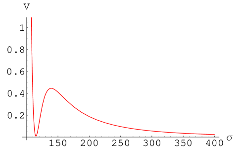
Figure 1: A plot of the potential (2.4) with values $a=.1$, $A=1$, $W_{0}=-10^{-4}$ and $D=3\times 10^{-9}$ in units of $M_{\rm Pl}$. The potential has been magnified by $5\times 10^{-10}$.

III The Cosmology of Wrapped Brane Gases

We are interested in studying the cosmology of a Universe filled with a gas of wrapped $p$-branes and the energy of a single modulus field $\sigma$. Using the Dirac-Born-Infeld action Boehm:2002bm , one can derive the equation of state for a $p$-brane gas in a universe with $d$ spatial dimensions, obtaining

$$\mathscr{P}_{p}=\left[\frac{p+1}{d}v^{2}-\frac{p}{d}\right]\rho_{p}\,,$$ (3.5)

where $\mathscr{P}_{p}$ is the pressure of the gas and $\rho_{p}$ is the energy density. In the relativistic limit, the branes behave as ordinary relativistic matter, with equation of state $\mathscr{P}_{p}\simeq\rho_{p}/d$. However, in the non-relativistic limit (wrapped branes with $|v|<<1$) the equation of state becomes $\mathscr{P}_{p}\simeq(-p/d)\rho_{p}$.

We take as our ansatz a flat ($k=0$), $d+1$-dimensional, Friedmann-Robertson-Walker (FRW) universe, with metric

$$ds^{2}=-dt^{2}+a^{2}(t)\sum_{i=1}^{d}dx_{i}^{2}\,,$$ (3.6)

where $a(t)$ is the scale factor. The resulting equations of motion are the Friedmann equation,

$$H^{2}=\frac{16\pi G_{d+1}}{d(d-1)}\rho\,,$$ (3.7)

where $H$ is the Hubble parameter $H\equiv\dot{a}/a$, and the acceleration equation

$$\frac{\ddot{a}}{a}=-\frac{8\pi G_{d+1}}{d(d-1)}\left[(d-2)\rho+d\mathscr{P}\right]\,.$$ (3.8)

Here, $\rho$ and $\mathscr{P}$ are the total energy density and pressure (wrapped branes plus modulus field) respectively, and the $(d+1)$-dimensional Newton constant is given by $G_{d+1}$. We will discuss the equation of motion for the modulus field $\sigma$, momentarily.

Matter sources, obeying equation of state $\mathscr{P}=w\rho$, will redshift in the expanding space as

$$\rho\sim a^{-d(1+w)}\,,$$ (3.9)

so that wrapped $p$-branes with $w=-p/d$, satisfy

$$\rho_{wrapping}\sim a^{-(d-p)}\,,$$ (3.10)

while the kinetic energy of the $\varphi$ field obeys

$$\rho_{\varphi}\sim a^{-2d}\,,$$ (3.11)

Hence, kinetic energy always redshifts more rapidly than other matter sources. With sufficient cosmic friction this dissipation of the modulus kinetic energy can allow the field to be placed gently into the shallow minimum of its potential. Of course, if other matter sources are not present in sufficient quantities, it is possible for $\varphi$ to overshoot the minimum at $\varphi_{min}$ and to run off to infinity.

The authors of Phys.Rev.D70.126012 , explicitly showed that radiation can be used to slow down the modulus and lower it into the minimum of the potential. While radiation redshifts as $1/a^{4}$, from (3.10) we see that string and brane winding gases redshift much more slowly, as $1/a^{2}$ and $1/a$, respectively. This means that wall and string gases will be more efficient in stabilizing the modulus field than radiation. For radiation the scale factor evolves as $a\propto t^{1/2}$, whereas for wrapped membranes, $a\propto t^{2}$ (see Eq. (6.21)). Thus, the Hubble damping term in (3.12) will be more significant for walls (and wrapped strings) than radiation.

In the following example we take $d=3$. It is clear from $(\ref{act1})$, that the field $\sigma$ has a non-standard kinetic term. For our purposes it is convenient to switch to a canonically normalized field $\varphi$, with equation of motion

$$\ddot{\varphi}+dH\dot{\varphi}+V^{\prime}(\varphi)=0\,,$$ (3.12)

where a prime denotes differentiation with respect to the field $\varphi$. Specializing to $d=3$, we achieve this by defining $\varphi\equiv\sqrt{3/2}\ln\sigma$, yielding the canonical kinetic term ${1\over 2}(\partial\varphi)^{2}$. In terms of the new variable $\varphi$, the potential (2.3) then becomes

$$V(\varphi) = De^{-\sqrt{6}\varphi}$$ (3.13)

$$+ \frac{1}{2}ae^{-ae^{\sqrt{\frac{2}{3}}\varphi}-2\sqrt{\frac{2}{3}}\varphi}\Big{(}Ae^{-ae^{\sqrt{\frac{2}{3}}\varphi}}(1+\frac{1}{3}ae^{\sqrt{\frac{2}{3}}\varphi})$$

$$+ W_{0}\Big{)}\,.$$

We work with this potential for the balance of this paper . Because of this, if other sources are present in the early Universe (even in small amounts) they will quickly become dominant Phys.Rev.D70.126012 .

IV Cosmological Evolution

In our scenario the Universe experiences several possible distinct epochs, depending on the initial relative energy densities of the matter sources. The earliest epoch is potential energy dominated. The field initially has no kinetic energy and begins falling, from rest, on a steep part of the potential. The value of the potential is large, and the Universe expands rapidly. In this regime, the equations of motion may be approximated by

$$\dot{a} = a\sqrt{\frac{2V}{d(d-1)}}\,,$$

$$\ddot{\varphi} + V^{\prime}(\varphi)=0\,,$$ (4.14)

where we have set $8\pi G_{d+1}=1$. For the initial conditions $\varphi(t=0)=\varphi_{0}$, and $\dot{\varphi}=0$ the exact solutions are

$$a(t) = \exp{\frac{1}{\sqrt{d(d-1)}}\int_{\varphi_{0}}^{\varphi}\frac{\sqrt{V}(\varphi)d\varphi}{\sqrt{V(\varphi_{0})-V(\varphi)}}}$$ (4.15)

$$\varphi(t) = \int_{0}^{t}dt\,\sqrt{2(V(\varphi_{0})-V(\varphi)}\,.$$ (4.16)

Taking the time derivative of (4.16), we see that if the potential is steep, $\dot{\varphi}$ can be quite large and, therefore, the kinetic energy in the modulus can quickly become the dominant energy component. Because of this, the Universe rapidly becomes dominated by the kinetic energy of the field $\varphi$. During this epoch, the equations of motion are approximated by

$$\ddot{\varphi} + dH\dot{\varphi}=0\,$$

$$\dot{a} = a\sqrt{\frac{\dot{\varphi}^{2}}{d(d-1)}}\,,$$ (4.17)

which can be solved exactly for $\varphi$,

$$\varphi(t)-\varphi^{\prime}=\ln{\left(\sqrt{\frac{d}{(d-1)}}(t-t^{\prime})\right)}\,,$$ (4.18)

where $\varphi^{\prime}$ and $t^{\prime}$ are constants set by the initial conditions at the beginning of the kinetic energy dominated phase.

¿From (4.18), it is clear that the modulus field will grow large if there is nothing to stop it. However, when brane winding modes are present, the kinetic energy, which redshifts very quickly (as $1/a^{6}$), dissipates due to the cosmic friction generated by the presence of the string and wall gases. Assuming such sources exist in sufficient quantities, the modulus field can now be fixed. The Universe becomes dominated by the energy of the brane sources and, depending on the relative initial densities of strings and walls, several possibilities can arise. If the initial energy densities of all matter components are of comparable orders of magnitude then, when kinetic energy domination ends, if walls are present, they will almost always dominate over the other components. An interesting possibility (although requiring some fine tuning) is the case in which all forms of energy densities are allowed to dominate for a short time. Since this is the most intricate possibility, we will examine such a case numerically in the following section.

V Numerical Results

For the numerical analysis we wish to solve (3.8) together with (3.12) and we take initial conditions subject to the constraint equation (3.7) . Throughout, we work in units with $M_{\rm Pl}^{2}=(8\pi G)^{-1}=1$, and focus on a three-dimensional Universe ($d=3$). In this case the possible winding branes are $2$-branes and strings, for which the total energy density and pressure are given by

$$\rho = {1\over 2}\dot{\varphi}^{2}+V(\varphi)+\frac{\rho^{(0)}_{p2}}{a}+\frac{\rho^{(0)}_{p1}}{a^{2}}\,$$ (5.19)

$$\mathscr{P} = {1\over 2}\dot{\varphi}^{2}-V(\varphi)-\frac{2}{3}\frac{\rho^{(0)}_{p2}}{a}-\frac{1}{3}\frac{\rho^{(0)}_{p1}}{a^{2}}\,,$$ (5.20)

where $\rho^{(0)}_{p1}$ and $\rho^{(0)}_{p2}$ are the initial energy densities of the wrapped strings and walls, respectively.

We will use the same parameters for the potential (3.13) as  Phys.Rev.D70.126012 . The parameters are: $A=1.0$, ${a=0.1}$, $D=3\times 10^{-26}$, $W_{0}=-2.96\times 10^{13}$. For these values the potential has a true minimum at $\sigma_{min}=320$, or $\varphi_{min}\simeq 7.065$, with $V(\varphi_{min})\simeq 6.35\times 10^{-35}$. The barrier separating the minimum from asymptotic infinity is located at $\varphi\simeq 7.18$ and has a height of $6.28\times 10^{-34}$.

For initial conditions we take $a_{0}=1$, $\varphi_{0}=3$ and $\dot{\varphi}_{0}=0$. For the initial energy densities of string and $2$-brane winding matter we take $\rho_{p1}^{(0)}=\frac{15}{2}\rho_{p2}^{(0)}=5.20\times 10^{-6}M_{\rm Pl}^{4}$. These initial conditions lead to a bound example, where the brane and string sources are present in sufficient quantities to trap the modulus field in the minimum of the potential. We present an unbound case later.

A plot of the modulus field $\varphi$ as a function of time is given in Fig. (2).

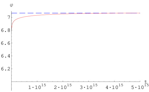
Figure 2: The time evolution of the modulus field $\varphi$ (solid red line). The field becomes trapped in the minimum of the potential at the value $\varphi_{min}=7.065$ (marked by the blue dotted line).

The relative energy densities $\rho_{i}$ of the moduli kinetic energy, potential, string and membrane sources are plotted as functions of the scale factor $a$ in Fig. (3).

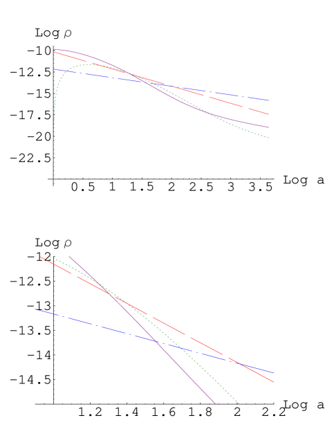
Figure 3: Top: The early time evolution of the various energy densities. The Universe starts out potential dominated (solid purple line), then kinetic energy dominated (dotted green), followed by string domination (dashed red) and finally wall domination (alternating dash-dot blue). Bottom: Here we zoom in to see better the transitions from potential, to kinetic, to string and finally to wall domination.

Initially the Universe is dominated by potential energy, then modulus kinetic energy, followed by the string gas and then the domain walls, which redshift most slowly, as $1/a$. During wall domination the Universe inflates, since $a\sim t^{2}$. Eventually, if the walls vanish, the Universe will become potential dominated again. We will comment more on this wall inflationary epoch in the next section.

As an example of an unbound case, we drastically dilute the energy densities of our initial sources to $\rho_{p1}^{(0)}=\rho_{p2}^{(0)}=10^{-10}M_{\rm Pl}^{4}$. All other parameters are left unchanged. The resulting behavior of the modulus field and relative energy densities are plotted in Fig. (4).

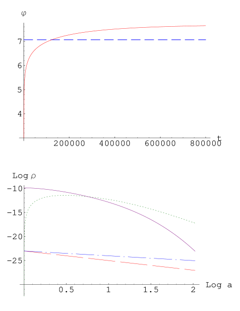
Figure 4: Top: Time evolution of the modulus field in the unbound case. The initial energy densities of strings and branes are not sufficient to trap $\varphi$. The field rolls past the local minimum of the potential, marked by the dotted line. Bottom: The early time evolution of the various energy densities for this unbound case.

VI The Inflationary Epoch

We have argued that, in the context of our scenario, the Universe will inevitably become dominated by a gas of wrapped membranes. In general, a gas of wrapped $p$-branes in $d$-dimensions has equation of state parameter $w=-p/d$ (recall Eq. (3.5)). Using (3.7) and (3.8), we see that his leads to scale factor evolution of the form

$$a(t)\propto t^{2/(d-p)}\,.$$ (6.21)

Therefore, a gas of co-dimension-one branes ($p=d-1$) will naturally lead to power-law inflation with $a(t)\sim t^{2}$, as long as the separation of the branes is much smaller than the Hubble radius. The resulting accelerated expansion will blow up the curvature radius of the branes (relative to the Hubble radius) and the inflationary period will end. Hence, there is no graceful exit problem in this scenario Phys.Rev.D69.083502 . Specifically, when the correlation length of the wall network $\xi(t)$ is comparable to $H^{-1}(t)=[(d-p)/2]t$, the brane gas approximation breaks down, since the distribution of the branes averaged over a Hubble expansion time becomes inhomogeneous, and the accelerated expansion will end. One can then show that, if the the ratio of the fundamental scale $m_{f}$ to the string scale $m_{s}$ is sufficiently large, $m_{f}/m_{s}\geq 10^{12}$, it is possible to obtain more than the 55-e-foldings required to solve the classic problems of the standard Big-Bang model Phys.Rev.D69.083502 .

During inflation, the co-moving Hubble length $H^{-1}/a$ is decreasing with time,

$$\frac{d}{dt}\frac{H^{-1}}{a}<0\,.$$ (6.22)

In our scenario, there are two periods of accelerated expansion ($\ddot{a}>0$). The first is during the potential dominated phase (our initial state), during which the equations of motion are given by (4.14). This initial inflationary period is quite short. The modulus field $\varphi$ picks up speed, the accelerating period ends, the co-moving Hubble length increases and the Universe passes into the kinetic energy dominated phase. The second phase of accelerated expansion is substatially longer, and begins during the wall dominated epoch . This behavior of the co-moving Hubble length is clearly seen in Fig. (5).

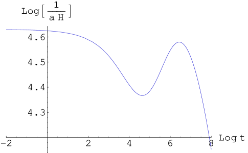
Figure 5: Behavior of the co-moving Hubble radius versus time. The Universe accelerates when the slope of this curve is negative.

Three difficult obstacles remain. The first is a generalized domain wall problem. Since the membranes cause the Universe to expand as $a(t)\propto t^{2}$, rather than like radiation with $a(t)\propto t^{1/2}$, a wall dominated period would drastically affect the abundance of light elements produced during nucleosynthesis. Besides this, if today even one wall (with a tension $\geq$ the electroweak scale) were present, it would overclose the Universe. Thus, a Universe containing walls must get rid of them eventually.

A second, possibly related problem, is how to reheat the Universe after the wall dominated period, in order to enter into a hot, radiation dominated Universe. Finally, it seems very unlikely that a wall accelerated Universe can produce the observed density fluctuations and microwave anisotropies, since the scalar index for wall inflation is given by

$$n_{s}-1=-\frac{2}{\alpha}\,,$$ (6.23)

where $\alpha=2/(d-p)$. Therefore, walls in $d=3$ give $n_{s}=0$ Phys.Rev.D69.083502 . This deviates significantly from the observed value (e.g., from WMAPext + 2dF) of $n_{s}=0.97\pm 0.03$ ($68\%$ confidence level) Phys.Lett.B592.1 .

VII Discussion

We have shown that wrapped brane and/or string gases in the early Universe provide an efficient mechanism for resolving the cosmological moduli stabilization problem. Such an initial state seems quite natural in the context of string theory and, in particular, may be relevant to the Brane Gas picture of string cosmology hep-th/0005212 . While some progress has been made in formulating the scenario in the context of compactification manifolds compatible with realistic particle physics Easson:2001fy ; hep-th/0212151 ; Easther:2002mi , the Brane Gas picture may greatly benefit from the mechanism suggested here .

In addition to the stabilization of moduli, we have presented a cosmological scenario that has an attractive way of generating an inflationary epoch in the early Universe, with a natural graceful exit mechanism. This phase of accelerated expansion is generated by a gas of wrapped membranes. However, as mentioned in the previous section, this cosmological scenario suffers from three remaining problems.

The first is the domain wall problem. The simplest possible solution is to simply not include walls in the picture in the first place. Such an initial condition is compatible with the original Brandenberger-Vafa picture presented in Nucl.Phys.B316.391 , in which the initial state of the Universe contains only strings. This also seems to be a natural starting point within the context of the Type IIB corner of the string moduli space, since the IIB theory does not admit stable two-branes. Using only a gas of string winding modes will suffice to stabilize the modulus field by our mechanism. The only downside of this picture is that a separate mechanism for inflating the Universe is needed .

A second possibility is to have the walls decay at some point after inflation. If the walls decay into radiation, this would also provide our scenario with a reheating mechanism (avoiding another obstacle). Several ways in which this can happen are discussed in Phys.Rev.D69.083502 . We briefly summarize them here. One possibility is that the branes are stabilized embedded branes, which decay once the temperature of the plasma drops sufficiently Phys.Lett.B467.205 ; Phys.Rev.D67.043504 . Another possibility is that the branes collide with anti-branes and annihilate, or if holes nucleate in the branes and expand at the speed of light, disolving them Seckel:1984ix . Since this would occur after inflation, there would be no causal obstruction to the local decay of sub-Hubble-volume brane networks. A final possibility was recently proposed by Stojkovic, Freese and Starkman hep-ph/0505026 . A sufficient abundance of primordial black holes can perforate domain walls and then the holes in the walls can grow and destroy the walls altogether.

Another problem with our cosmological scenario is how to generate a scale invariant spectrum of density perturbations. This seems impossible to do within the context of wall inflation without introducing some sort of new physics.

Finally, we note that it is possible to obtain slow-roll inflation once the potential begins to dominate (after the walls are gone). One can tune the potential so that the barrier is very flat at the top. An example of this is provided using the imaginary component (the axion) of the volume modulus $\varphi$ hep-th/0406230 . A second condition required to build a successful model, is that the initial conditions would have to be tuned so that the wall and string winding gases place the modulus gently at the top of the barrier. In such a model, the modulus itself could act as the inflaton and generate a scale invariant spectrum. We leave more detailed explorations of the above speculations to future research projects.

Note Added

As this work was being written up, we became aware of related work, also almost completed. This work has since appeared hep-th/0505151 , and contains results which have some overlap with those presented here.

References

- (1) M. Dine and N. Seiberg, Phys. Lett. B 162, 299 (1985).
- (2) R. Brustein and P. J. Steinhardt, Phys. Lett. B 302, 196 (1993) [arXiv:hep-th/9212049].
- (3) S. Alexander, R. H. Brandenberger and D. Easson, Phys. Rev. D 62, 103509 (2000) [arXiv:hep-th/0005212].
- (4) R. Brandenberger, D. A. Easson and D. Kimberly, Nucl. Phys. B 623, 421 (2002) [arXiv:hep-th/0109165].
- (5) A. Albrecht, C. P. Burgess, F. Ravndal and C. Skordis, Phys. Rev. D 65, 123507 (2002) [arXiv:astro-ph/0107573].
- (6) G. N. Felder, A. V. Frolov, L. Kofman and A. V. Linde, Phys. Rev. D 66, 023507 (2002) [arXiv:hep-th/0202017].
- (7) T. Barreiro, B. de Carlos and E. J. Copeland, Phys. Rev. D 58, 083513 (1998) [arXiv:hep-th/9805005].
- (8) T. Barreiro, B. de Carlos and N. J. Nunes, Phys. Lett. B 497, 136 (2001) [arXiv:hep-ph/0010102].
- (9) R. Brustein, S. P. de Alwis and P. Martens, Phys. Rev. D 70, 126012 (2004) [arXiv:hep-th/0408160].
- (10) R. Brandenberger, D. A. Easson and A. Mazumdar, Phys. Rev. D 69, 083502 (2004) [arXiv:hep-th/0307043].
- (11) F. A. Brito, F. F. Cruz and J. F. N. Oliveira, Phys. Rev. D 71, 083516 (2005) [arXiv:hep-th/0502057].
- (12) S. Kachru, R. Kallosh, A. Linde and S. P. Trivedi, Phys. Rev. D 68, 046005 (2003) [arXiv:hep-th/0301240].
- (13) T. Boehm and R. Brandenberger, JCAP 0306, 008 (2003) [arXiv:hep-th/0208188].
- (14) S. Eidelman et al. [Particle Data Group], Phys. Lett. B 592, 1 (2004).
- (15) D. A. Easson, Int. J. Mod. Phys. A 18, 4295 (2003) [arXiv:hep-th/0110225].
- (16) S. H. S. Alexander, JHEP 0310, 013 (2003) [arXiv:hep-th/0212151].
- (17) R. Easther, B. R. Greene and M. G. Jackson, Phys. Rev. D 66, 023502 (2002) [arXiv:hep-th/0204099].
- (18) S. Watson and R. Brandenberger, JCAP 0311, 008 (2003) [arXiv:hep-th/0307044].
- (19) S. Watson, Phys. Rev. D 70, 066005 (2004) [arXiv:hep-th/0404177].
- (20) A. Kaya, JCAP 0408, 014 (2004) [arXiv:hep-th/0405099].
- (21) A. J. Berndsen and J. M. Cline, Int. J. Mod. Phys. A 19, 5311 (2004) [arXiv:hep-th/0408185].
- (22) S. Arapoglu and A. Kaya, Phys. Lett. B 603, 107 (2004) [arXiv:hep-th/0409094].
- (23) S. Watson, arXiv:hep-th/0409281.
- (24) R. Brandenberger, Y. K. Cheung and S. Watson, arXiv:hep-th/0501032.
- (25) T. Rador, arXiv:hep-th/0501249.
- (26) T. Rador, arXiv:hep-th/0502039.
- (27) S. P. Patil and R. H. Brandenberger, arXiv:hep-th/0502069.
- (28) T. Rador, arXiv:hep-th/0504047.
- (29) S. P. Patil, arXiv:hep-th/0504145.
- (30) A. Kaya, arXiv:hep-th/0504208.
- (31) R. H. Brandenberger and C. Vafa, Nucl. Phys. B 316, 391 (1989).
- (32) S. Alexander, R. Brandenberger and M. Rozali, arXiv:hep-th/0302160.
- (33) R. Brandenberger, D. A. Easson and A. Mazumdar, Phys. Rev. D 69, 083502 (2004) [arXiv:hep-th/0307043].
- (34) T. Biswas, R. Brandenberger, D. A. Easson and A. Mazumdar, Phys. Rev. D 71, 083514 (2005) [arXiv:hep-th/0501194].
- (35) M. Nagasawa and R. H. Brandenberger, Phys. Lett. B 467, 205 (1999) [arXiv:hep-ph/9904261].
- (36) M. Nagasawa and R. Brandenberger, Phys. Rev. D 67, 043504 (2003) [arXiv:hep-ph/0207246].
- (37) D. Seckel, Prepared for Inner Space/ Outer Space: Conference on Physics at the Interface of Astrophysics / Cosmology and Particle Physics, Batavia, Illinois, 2-5 May 1984
- (38) D. Stojkovic, K. Freese and G. D. Starkman, arXiv:hep-ph/0505026.
- (39) J. J. Blanco-Pillado et al., JHEP 0411, 063 (2004) [arXiv:hep-th/0406230].
- (40) A. Berndsen, T. Biswas and J. M. Cline, arXiv:hep-th/0505151.