Abstract

Certain aspects of the integrability/solvability of the Calogero-Sutherland-Moser systems and the Ruijsenaars-Schneider-van Diejen systems with rational and trigonometric potentials are reviewed. The equilibrium positions of classical multi-particle systems and the eigenfunctions of single-particle quantum mechanics are described by the same orthogonal polynomials: the Hermite, Laguerre, Jacobi, continuous Hahn, Wilson and Askey-Wilson polynomials. The Hamiltonians of these single-particle quantum mechanical systems have two remarkable properties, factorization and shape invariance.

1 Introduction

Exactly solvable or quasi-exactly solvable multi-particle quantum mechanical systems have many remarkable properties. Especially, those of the Calogero-Sutherland-Moser(CSM) systems[1, 2, 3] and their integrable deformation called the Ruijsenaars-Schneider-van Diejen (RSvD) systems [4, 5] have been well studied. For example, the spectral curves of the classical elliptic CSM systems appear in the Seiberg-Witten theory of the supersymmetric gauge theory [6], and the relation between the eigenstates of the quantum Sutherland system and those of the Ruijsenaars-Schneider system has led to the discovery of the deformed Virasoro and $W_{N}$ algebras [7].

The equilibrium positions of the Calogero-Sutherland systems are described by the zeros of the classical orthogonal polynomials; the Hermite, Laguerre and Jacobi (Chebyshev, Legendre, Gegenbauer) polynomials [8, 9, 10, 11]. Motivated by the simple reasoning illustrated in the following diagram (a similar idea has led to the deformed Virasoro and $W_{N}$ algebras),

 Calogero-Sutherland systems $$\smash{\mathop{\hbox to128.0374pt{\rightarrowfill}}\limits^{\mbox{equilibrium positions}}}$$ classical orthogonal polynomials

$$\Bigg{\downarrow}\hbox to0.0pt{$\vbox{\hbox{$\scriptstyle\mbox{`good' deformation}$}}$\hss}\hskip 56.9055pt \hskip 42.67912pt\Bigg{\downarrow}\hbox to0.0pt{$\vbox{\hbox{$\scriptstyle\makebox{ \shortstack{`good' deformation \\ expected}}$}}$\hss}$$

Ruijsenaars-Schneider -van Diejen systems $$\smash{\mathop{\hbox to128.0374pt{\rightarrowfill}}\limits^{\mbox{equilibrium positions}}}$$ deformed classical orthogonal polynomials

we studied the equilibrium positions of the RSvD systems with rational and trigonometric potentials by using numerical analysis, functional equation and three-term recurrence. This program worked well and we obtained the deformed polynomials [12, 13] (see also [14, 15, 16]), which fitted in the Askey-scheme of the hypergeometric orthogonal polynomials [17, 18, 19]: deformation of the Hermite polynomial $\Rightarrow$ special cases of the Meixner-Pollaczek polynomial and the continuous Hahn polynomial; deformation of the Laguerre polynomial $\Rightarrow$ the continuous dual Hahn polynomial and the Wilson polynomial; deformation of the Jacobi polynomial $\Rightarrow$ the Askey-Wilson polynomial.

The Hermite, Laguerre and Jacobi polynomials, which describe the equilibrium positions of the classical multi-particle CS systems, also describe the eigenfunctions of the corresponding single-particle quantum CS systems. This interesting property is inherited by the deformed ones. The continuous Hahn, Wilson and Askey-Wilson polynomials, which describe the equilibrium positions of the classical multi-particle RSvD systems, also describe the eigenfunctions of the corresponding single-particle quantum RSvD systems. The Hamiltonians for single-particle quantum CS and RSvD systems have two remarkable properties, factorization and shape invariance [20, 21, 22, 23, 24]. Shape invariance is an important ingredient of many exactly solvable quantum mechanics. In our case the shape invariance determines the eigenfunctions and spectrum from the data of the ground state wavefunction and the energy of the first excited state [25, 13].

The aim of this note is to give a comprehensive review of the above facts; (a) equilibrium positions and single-particle eigenfunctions of the CS and RSvD systems with rational and trigonometric potentials are described by the same orthogonal polynomials, (b) Hamiltonians for quantum single-particle CS and RSvD systems with rational and trigonometric potentials have two properties, factorization and shape invariance.

This note is organized as follows. In section 2 we recapitulate the essence of the models, CS and RSvD systems with rational and trigonometric potentials. The relationship between CS and RSvD systems is discussed, and the equations for the equilibrium positions are given. In sections 3–6 we demonstrate that the same polynomials appear in the equilibrium positions and single-particle eigenfunctions. We emphasize the shape invariance of the single-particle Hamiltonian along the idea of Crum[21]. In section 3 the CS and RSvD systems with rational $A$-type potentials are discussed and the relevant polynomials are the Hermite and the continuous Hahn polynomials. In section 4 rational $BC$-type potentials are discussed and the Laguerre and Wilson polynomials play the role. Section 5 is for the trigonometric $A$-type potentials. In section 6 the trigonometric $BC$-type potentials are discussed and the Jacobi and Askey-Wilson polynomials appear. Section 7 is for summary and comments.

2 Models

We recapitulate the basics of the models and present the equations for their equilibrium positions. A multi-particle quantum (or classical) mechanics governed by a Hamiltonian $H(p,q)$ (or classical one $H^{\rm class}(p,q)$) is considered. The dynamical variables are real-valued coordinates $q={}^{t}(q_{1},\cdots,q_{n})$ and their canonically conjugate momenta $p={}^{t}(p_{1},\cdots,p_{n})$. For quantum case we have $p_{j}=-i\hbar\frac{\partial}{\partial q_{j}}$. We keep dimensionful parameters, e.g. mass, angular frequency, the Planck constant, etc. The coordinate $q_{j}$ has dimension of length.

2.1 Calogero-Sutherland Systems

The Hamiltonian of the Calogero-Sutherland (CS) systems is

$$H_{\rm CS}(p,q)=\sum_{j=1}^{n}\frac{1}{2m}p_{j}^{2}+V_{\rm CS}(q)\,,$$ (1)

where the potential $V_{\rm CS}(q)$ can be written in terms of the prepotential $W(q)$,

$$V_{\rm CS}(q)=\sum_{j=1}^{n}\frac{1}{2m}\biggl{(}\Bigl{(}\frac{\partial W(q)}{\partial q_{j}}\Bigr{)}^{2}+\hbar\,\frac{\partial^{2}W(q)}{\partial q_{j}^{2}}\biggr{)}\,.$$ (2)

The explicit forms of the potential $V_{\rm CS}(q)$ and the prepotential $W(q)$ are as follows:
(i) rational $A_{n-1}$ :

$$V_{\rm CS}(q) =\sum_{j=1}^{n}\frac{1}{2}m\omega^{2}q_{j}^{2}+\frac{\hbar^{2}}{2m}\sum_{\genfrac{}{}{0.0pt}{2}{j,k=1}{j\neq k}}^{n}\frac{g(g-1)}{(q_{j}-q_{k})^{2}}-\tfrac{1}{2}\hbar\omega n\bigl{(}1+g(n-1)\bigr{)}\,,$$ (3)

$$W(q) =-\sum_{j=1}^{n}\frac{1}{2}m\omega q_{j}^{2}+\sum_{1\leq j<k\leq n}g\hbar\log\sqrt{\tfrac{m\omega}{\hbar}}\,\bigl{|}q_{j}-q_{k}\bigr{|}\,,$$ (4)

(ii) rational $BC_{n}$ :

$$V_{\rm CS}(q) =\sum_{j=1}^{n}\biggl{(}\frac{1}{2}m\omega^{2}q_{j}^{2}+\frac{\hbar^{2}}{2m}\frac{(g_{S}+g_{L})(g_{S}+g_{L}-1)}{q_{j}^{2}}\biggr{)}$$

$$\quad+\frac{\hbar^{2}}{2m}\sum_{\genfrac{}{}{0.0pt}{2}{j,k=1}{j\neq k}}^{n}\biggl{(}\frac{g_{M}(g_{M}-1)}{(q_{j}-q_{k})^{2}}+\frac{g_{M}(g_{M}-1)}{(q_{j}+q_{k})^{2}}\biggr{)}-\hbar\omega n\bigl{(}g_{S}+g_{L}+\tfrac{1}{2}+g_{M}(n-1)\bigr{)}\,,$$ (5)

$$W(q) =-\sum_{j=1}^{n}\frac{1}{2}m\omega q_{j}^{2}+\sum_{1\leq j<k\leq n}g_{M}\hbar\Bigl{(}\log\sqrt{\tfrac{m\omega}{\hbar}}\,\bigl{|}q_{j}-q_{k}\bigr{|}+\log\sqrt{\tfrac{m\omega}{\hbar}}\,\bigl{|}q_{j}+q_{k}\bigr{|}\Bigr{)}$$

$$\quad+\sum_{j=1}^{n}\Bigl{(}g_{S}\hbar\log\sqrt{\tfrac{m\omega}{\hbar}}\,\bigl{|}q_{j}\bigr{|}+g_{L}\hbar\log\sqrt{\tfrac{m\omega}{\hbar}}\,\bigl{|}2q_{j}\bigr{|}\Bigr{)}\,,$$ (6)

(iii) trigonometric $A_{n-1}$ :

$$V_{\rm CS}(q) =\frac{\hbar^{2}\pi^{2}}{2mL^{2}}\sum_{\genfrac{}{}{0.0pt}{2}{j,k=1}{j\neq k}}^{n}\frac{g(g-1)}{\sin^{2}\frac{\pi}{L}(q_{j}-q_{k})}-\frac{\hbar^{2}\pi^{2}}{2mL^{2}}g^{2}\frac{1}{3}n(n^{2}-1)\,,$$ (7)

$$W(q) =\sum_{1\leq j<k\leq n}g\hbar\log\bigl{|}\sin\tfrac{\pi}{L}(q_{j}-q_{k})\bigr{|}\,,$$ (8)

(iv) trigonometric $BC_{n}$ :

$$V_{\rm CS}(q) =\frac{\hbar^{2}\pi^{2}}{2mL^{2}}\sum_{j=1}^{n}\biggl{(}\frac{(g_{S}+g_{L})(g_{S}+g_{L}-1)}{\sin^{2}\frac{\pi}{L}q_{j}}+\frac{g_{L}(g_{L}-1)}{\cos^{2}\frac{\pi}{L}q_{j}}\biggl{)}$$

$$\quad+\frac{\hbar^{2}\pi^{2}}{2mL^{2}}\sum_{\genfrac{}{}{0.0pt}{2}{j,k=1}{j\neq k}}^{n}\biggl{(}\frac{g_{M}(g_{M}-1)}{\sin^{2}\frac{\pi}{L}(q_{j}-q_{k})}+\frac{g_{M}(g_{M}-1)}{\sin^{2}\frac{\pi}{L}(q_{j}+q_{k})}\biggr{)}$$

$$\quad-\frac{\hbar^{2}\pi^{2}}{2mL^{2}}n\Bigl{(}\bigl{(}g_{S}+2g_{L}+g_{M}(n-1)\bigr{)}^{2}+g_{M}^{2}\tfrac{1}{3}(n^{2}-1)\Bigr{)}\,,$$ (9)

$$W(q) =\sum_{1\leq j<k\leq n}g_{M}\hbar\Bigl{(}\log\bigl{|}\sin\tfrac{\pi}{L}(q_{j}-q_{k})\bigr{|}+\log\bigl{|}\sin\tfrac{\pi}{L}(q_{j}+q_{k})\bigr{|}\Bigr{)}$$

$$\quad+\sum_{j=1}^{n}\Bigl{(}g_{S}\hbar\log\bigl{|}\sin\tfrac{\pi}{L}q_{j}\bigr{|}+g_{L}\hbar\log\bigl{|}\sin\tfrac{\pi}{L}2q_{j}\bigr{|}\Bigr{)}\,.$$ (10)

The constant terms in $V_{\rm CS}(q)$ are the consequences of the expression (2) in terms of the prepotential. A constant shift of $W(q)$ does not affect (2). In those formulas $g,g_{S},g_{M}$ and $g_{L}$ are dimensionless couplings constants and we assume they are positive. The other notation is conventional; $m$ is the mass of particles, $\omega$ is the angular frequency, $\hbar$ is the Planck constant (divided by $2\pi$) and $L$ is the circumference. All these parameters are positive.

2.2 Ruijsenaars-Schneider-van Diejen Systems

The Ruijsenaars-Schneider-van Diejen (RSvD) systems are deformation of the Calogero-Sutherland-Moser systems. The Hamiltonian of RSvD systems is

$$H(p,q)=\frac{1}{2}mc^{2}\sum_{j=1}^{n}\Bigl{(}\sqrt{V_{j}(q)}\,e^{\frac{1}{mc}p_{j}}\sqrt{{V_{j}(q)}^{*}}+\sqrt{{V_{j}(q)}^{*}}\,e^{-\frac{1}{mc}p_{j}}\sqrt{V_{j}(q)}-V_{j}(q)-{V_{j}(q)}^{*}\Bigr{)}\,,$$ (11)

where $V_{j}(q)$ are

$$V_{j}(q)=w(q_{j})\prod_{\genfrac{}{}{0.0pt}{2}{k=1}{k\neq j}}^{n}v(q_{j}-q_{k})\times\begin{cases}1&\text{for $A_{n-1}$}\\ v(q_{j}+q_{k})&\text{for $BC_{n}$}\,.\end{cases}$$ (12)

Since operators $e^{\pm\frac{1}{mc}p_{j}}=e^{\mp i\frac{\hbar}{mc}\frac{\partial}{\partial q_{j}}}$ cause finite shifts of the wavefunction in the imaginary direction ($e^{\pm\frac{1}{mc}p_{j}}f(q)=f(q_{1},\cdots,q_{j}\mp i\frac{\hbar}{mc},\cdots,q_{n})$), we call these systems ‘discrete’ dynamical systems. The basic potential functions $v(x)$ and $w(x)$ are given by as follows:
(i) rational $A_{n-1}$ :

$$v(x) =1-i\frac{\hbar}{mc}\frac{g}{x}\,,$$ (13)

$$w(x) =\Bigl{(}1+i\,\frac{\omega_{1}}{c}\,x\Bigr{)}\Bigl{(}1+i\,\frac{\omega_{2}}{c}\,x\Bigr{)}\,,$$ (14)

(ii) rational $BC_{n}$ :

$$v(x) =1-i\frac{\hbar}{mc}\frac{g_{0}}{x}\,,$$ (15)

$$w(x) =\Bigl{(}1+i\,\frac{\omega_{1}}{c}\,x\Bigr{)}\Bigl{(}1+i\,\frac{\omega_{2}}{c}\,x\Bigr{)}\Bigl{(}1-i\frac{\hbar}{mc}\frac{g_{1}}{x}\Bigr{)}\Bigl{(}1-i\frac{\hbar}{mc}\frac{g_{2}}{x-i\frac{\hbar}{2mc}}\Bigr{)}\,,$$ (16)

(iii) trigonometric $A_{n-1}$ :

$$v(x) =\frac{\sin\frac{\pi}{L}(x-i\frac{\hbar}{mc}g)}{\sin\frac{\pi}{L}x}\,,$$ (17)

$$w(x) =1\,,$$ (18)

(iv) trigonometric $BC_{n}$ :

$$v(x) =\frac{\sin\frac{\pi}{L}(x-i\frac{\hbar}{mc}g_{0})}{\sin\frac{\pi}{L}x}\,,$$ (19)

$$w(x) =\frac{\sin\frac{\pi}{L}(x-i\frac{\hbar}{mc}g_{1})}{\sin\frac{\pi}{L}x}\,\frac{\sin\frac{\pi}{L}(x-i\frac{\hbar}{2mc}-i\frac{\hbar}{mc}g_{2})}{\sin\frac{\pi}{L}(x-i\frac{\hbar}{2mc})}$$

$$\quad\times\frac{\cos\frac{\pi}{L}(x-i\frac{\hbar}{mc}g^{\prime}_{1})}{\cos\frac{\pi}{L}x}\,\frac{\cos\frac{\pi}{L}(x-i\frac{\hbar}{2mc}-i\frac{\hbar}{mc}g^{\prime}_{2})}{\cos\frac{\pi}{L}(x-i\frac{\hbar}{2mc})}\,.$$ (20)

Here $g,g_{0},g_{1},g_{2},g^{\prime}_{1}$ and $g^{\prime}_{2}$ are dimensionless couplings constants and $c$ is the (fictitious) speed of light. We assume they are all positive.

Let us consider $c\rightarrow\infty$ limit, in which RSvD systems reduce to CS systems. Since $v(x)$ and $w(x)$ contains $c$ and $i$ as a combination $\frac{i}{c}$, we can expand them as follows:

$$v(x) =1+\tfrac{i}{c}\,v_{1}(x)+(\tfrac{i}{c})^{2}v_{2}(x)+O(\tfrac{1}{c^{3}})\,,$$ (21)

$$w(x) =1+\tfrac{i}{c}\,w_{1}(x)+(\tfrac{i}{c})^{2}w_{2}(x)+O(\tfrac{1}{c^{3}})\,.$$ (22)

Here $v_{1}(x)$ and $w_{1}(x)$ are odd real functions and $v_{2}(x)$ and $w_{2}(x)$ are even real functions because of $v(x)^{*}=v(-x)$ and $w(x)^{*}=w(-x)$. Then the Hamiltonian (11) has the expansion,

$$H(p,q) =\sum_{j=1}^{n}\frac{1}{2m}p_{j}^{2}+\sum_{j=1}^{n}\Bigl{(}\frac{m}{2}w_{1}(q_{j})^{2}-\frac{\hbar}{2}w^{\prime}_{1}(q_{j})\Bigr{)}$$

$$\quad+\sum_{\genfrac{}{}{0.0pt}{2}{j,k=1}{j\neq k}}^{n}\Bigl{(}\frac{m}{2}v_{1}(q_{j}-q_{k})^{2}-\frac{\hbar}{2}v^{\prime}_{1}(q_{j}-q_{k})+\frac{m}{2}v_{1}(q_{j}+q_{k})^{2}-\frac{\hbar}{2}v^{\prime}_{1}(q_{j}+q_{k})$$

$$\qquad\qquad\quad+mw_{1}(q_{j})\bigl{(}v_{1}(q_{j}-q_{k})+v_{1}(q_{j}+q_{k})\bigr{)}\Bigr{)}$$

$$\quad+\sum_{\genfrac{}{}{0.0pt}{2}{j,k,l=1}{j\neq k\neq l\neq j}}^{n}\frac{m}{2}\bigl{(}v_{1}(q_{j}-q_{k})+v_{1}(q_{j}+q_{k})\bigr{)}\bigl{(}v_{1}(q_{j}-q_{l})+v_{1}(q_{j}+q_{l})\bigr{)}+O\Bigl{(}\frac{1}{c}\Bigr{)}\,,$$ (23)

where the prime stands for the derivative. (For $A_{n-1}$ type systems, the terms containing $v_{1}(q_{j}+q_{k})$ and $v^{\prime}_{1}(q_{j}+q_{k})$ should be omitted.) By explicit calculation, we obtain

$$\lim_{c\rightarrow\infty}H(p,q)=H_{\rm CS}(p,q),$$ (24)

where the correspondence of parameters are

(i) $$\omega_{1}+\omega_{2}=\omega,\quad g=g,$$ (25)

(ii) $$\omega_{1}+\omega_{2}=\omega,\quad g_{0}=g_{M},\quad g_{1}+g_{2}=g_{S}+g_{L},$$ (26)

(iii) $$g=g,$$ (27)

(iv) $$g_{0}=g_{M},\quad g_{1}+g_{2}=g_{S}+g_{L},\quad g^{\prime}_{1}+g^{\prime}_{2}=g_{L}\,.$$ (28)

2.3 Equilibrium Positions

The classical Hamiltonian $H^{\rm class}(p,q)$ is obtained from the quantum one $H(p,q)$ by the following procedure; (a) regard $p_{j}$ is a $c$-number, (b) after expressing dimensionless coupling constants $g,g_{1},g_{2},\cdots$ by dimensionful coupling constants $\bar{g}=g\hbar,{\bar{g}}_{1}=g_{1}\hbar,{\bar{g}}_{2}=g_{2}\hbar,\cdots$, assume $\bar{g},{\bar{g}}_{1},{\bar{g}}_{2},\cdots$ are independent of $\hbar$, (c) take $\hbar\rightarrow 0$ limit. In the same way, $V^{\rm class}(q)$, $W^{\rm class}(q)$, $V_{j}^{\rm class}(q)$, $v^{\rm class}(x)$ and $w^{\rm class}(x)$ are also obtained.

The canonical equations of motion of the classical systems are

$$\frac{dq_{j}}{dt}=\frac{\partial H^{\rm class}(p,q)}{\partial p_{j}}\,,\quad\frac{dp_{j}}{dt}=-\frac{\partial H^{\rm class}(p,q)}{\partial q_{j}}\,.$$ (29)

The equilibrium positions are the stationary solution

$$p=0\,,\quad q=\bar{q}\,,$$ (30)

in which $\bar{q}$ satisfies

$$\frac{\partial H^{\rm class}(0,q)}{\partial q_{j}}\Biggm{|}_{q=\bar{q}}=0\qquad(j=1,\ldots,n).$$ (31)

For CS system, (31) becomes $\frac{\partial V^{\rm class}_{\rm CS}(q)}{\partial q_{j}}\Bigm{|}_{q=\bar{q}}=0$ and it is equivalent to the condition [27]

$$\frac{\partial W^{\rm class}(q)}{\partial q_{j}}\Biggm{|}_{q=\bar{q}}=0\qquad(j=1,\ldots,n).$$ (32)

For RSvD system, (31) is equivalent to the condition [14]

$$V_{j}^{\rm class}(\bar{q})=V_{j}^{\rm class}(\bar{q})^{*}>0\qquad(j=1,\ldots,n).$$ (33)

This equation without inequality is rewritten in a Bethe ansatz like equation

$$\prod_{\genfrac{}{}{0.0pt}{2}{k=1}{k\neq j}}^{n}\frac{v^{\rm class}(\bar{q}_{j}-\bar{q}_{k})\,v^{\rm class}(\bar{q}_{j}+\bar{q}_{k})}{v^{\rm class}(\bar{q}_{j}-\bar{q}_{k})^{*}\,v^{\rm class}(\bar{q}_{j}+\bar{q}_{k})^{*}}=\frac{w^{\rm class}(\bar{q}_{j})^{*}}{w^{\rm class}(\bar{q}_{j})}\qquad(j=1,\ldots,n).$$ (34)

(For $A_{n-1}$ type systems, $v^{\rm class}(\bar{q}_{j}+\bar{q}_{k})$ and $v^{\rm class}(\bar{q}_{j}+\bar{q}_{k})^{*}$ should be omitted.)

3 Rational $A$ Types

In this section we consider CS and RSvD systems with rational $A$ type potentials. Relevant polynomials are the Hermite polynomial and the continuous Hahn polynomial.

3.1 Calogero Systems

The Hamiltonian is (1) with the potential (3)–(4).

3.1.1 Equilibrium positions of $n$-particle classical systems

For the $n$-particle prepotential (4), the equation for the equilibrium positions (32) was studied by Stieltjes in a slightly different context more than a century ago [9]. Let us consider a polynomial whose zeros give the equilibrium positions, $f(y)=\prod_{j=1}^{n}(y-\sqrt{\frac{m\omega}{\bar{g}}}\,\bar{q}_{j})$. Then (32) can be converted to a differential equation for $f(y)$, which is the determining equation for the Hermite polynomial. Therefore we obtain the result [8],

$$\prod_{j=1}^{n}\Bigl{(}y-\sqrt{\frac{m\omega}{\bar{g}}}\,\bar{q}_{j}\Bigr{)}=H_{n}^{\rm monic}(y)\,,$$ (35)

where $H_{n}(y)=2^{n}H_{n}^{\rm monic}(y)$ is the Hermite polynomial [18].

3.1.2 Eigenfunctions of single-particle quantum mechanics

Let us consider single-particle case ($n=1$) and write $x=q_{1}$. The Hamiltonian (1) describes the harmonic oscillator with the constant energy shift

$$H=-\frac{\hbar^{2}}{2m}\frac{d^{2}}{dx^{2}}+\frac{1}{2}m\omega^{2}x^{2}-\frac{1}{2}\hbar\omega\,.$$ (36)

The eigenfunctions of this Hamiltonian are well-known, but we describe it in detail in order to illustrate the idea of Crum[21], construction of isospectral Hamiltonians (see Figure 1). By introducing a dimensionless variable $y$,

$$y=\sqrt{\frac{m\omega}{\hbar}}x,$$ (37)

$H$ can be written as

$$H=\hbar\omega\mathcal{H}\,,\quad\mathcal{H}=-\frac{1}{2}\frac{d^{2}}{dy^{2}}+\frac{1}{2}y^{2}-\frac{1}{2}\,.$$ (38)

Instead of $H\phi_{n}=E_{n}\phi_{n}$, let us consider a rescaled one $\mathcal{H}\phi_{n}(y)=\mathcal{E}_{n}\phi_{n}(y)$ ($n=0,1,2,\ldots$), where energies are related as $E_{n}=\hbar\omega\mathcal{E}_{n}$.

Let us develop the factorization method in its fullest generality. Let us assume that a single-particle Hamiltonian $\mathcal{H}$ depends on a set of parameters to be represented collectively as $\bm{\lambda}$. The present Hamiltonian $\mathcal{H}$ (38) contains no parameter, though. The Hamiltonian $\mathcal{H}$, defined in terms of the prepotential, is factorizable:

$$\mathcal{H} =\mathcal{H}(y\,;\bm{\lambda})=\mathcal{A}(y\,;\bm{\lambda})^{\dagger}\mathcal{A}(y\,;\bm{\lambda})=\frac{1}{2}\Bigl{(}-\frac{d^{2}}{dy^{2}}+\Bigl{(}\frac{d\mathcal{W}(y\,;\bm{\lambda})}{dy}\Bigr{)}^{2}+\frac{d^{2}\mathcal{W}(y\,;\bm{\lambda})}{dy^{2}}\Bigr{)}\,,$$ (39)

$$\mathcal{A} =\mathcal{A}(y\,;\bm{\lambda})\stackrel{{\scriptstyle\rm def}}{{=}}\frac{1}{\sqrt{2}}\Bigl{(}-i\frac{d}{dy}+i\,\frac{d\,\mathcal{W}(y\,;\bm{\lambda})}{dy}\Bigr{)}\,,$$ (40)

$$\mathcal{A}^{\dagger} =\mathcal{A}(y\,;\bm{\lambda})^{\dagger}\stackrel{{\scriptstyle\rm def}}{{=}}\frac{1}{\sqrt{2}}\Bigl{(}-i\frac{d}{dy}-i\,\frac{d\,\mathcal{W}(y\,;\bm{\lambda})}{dy}\Bigr{)}\,,$$ (41)

where $\mathcal{W}(y\,;\bm{\lambda})$ is a prepotential. The ground state of $\mathcal{H}$ is annihilated by $\mathcal{A}$ (see Remark in §4.1.2) and it is expressed by $\mathcal{W}$,

$$\phi_{0}(y\,;\bm{\lambda})\propto e^{\mathcal{W}(y\,;\bm{\lambda})},\quad\mathcal{E}_{0}(\bm{\lambda})=0.$$ (42)

In the present case we have

$$\mathcal{W}(y)=-\frac{1}{2}y^{2},\quad\phi_{0}(y)\propto e^{-\frac{1}{2}y^{2}},$$ (43)

which is obviously square-integrable.

This Hamiltonian has a good property, shape invariance. Its key identity is

$$\mathcal{A}(y\,;\bm{\lambda})\mathcal{A}(y\,;\bm{\lambda})^{\dagger}=\mathcal{A}(y\,;\bm{\lambda}+\bm{\delta})^{\dagger}\mathcal{A}(y\,;\bm{\lambda}+\bm{\delta})+\mathcal{E}_{1}(\bm{\lambda})\,,$$ (44)

where $\bm{\delta}$ stands for a set of constants. In the present case we have

$$\mathcal{E}_{1}=1\,,$$ (45)

and there is no $\bm{\delta}$ because of no $\bm{\lambda}$. Starting from $\mathcal{A}_{0}=\mathcal{A}$, $\mathcal{H}_{0}=\mathcal{H}$ and $\phi_{0,n}=\phi_{n}$, let us define $\mathcal{A}_{s}$, $\mathcal{H}_{s}$ and $\phi_{s,n}$ ($n\geq s\geq 0$) recursively:

$$\mathcal{A}_{s+1}(y\,;\bm{\lambda}) \stackrel{{\scriptstyle\rm def}}{{=}}\mathcal{A}_{s}(y\,;\bm{\lambda}+\bm{\delta})\,,$$ (46)

$$\mathcal{H}_{s+1}(y\,;\bm{\lambda}) \stackrel{{\scriptstyle\rm def}}{{=}}\mathcal{A}_{s}(y\,;\bm{\lambda})\mathcal{A}_{s}(y\,;\bm{\lambda})^{\dagger}+\mathcal{E}_{s}(\bm{\lambda})\,,$$ (47)

$$\phi_{s+1,n}(y\,;\bm{\lambda}) \stackrel{{\scriptstyle\rm def}}{{=}}\mathcal{A}_{s}(y\,;\bm{\lambda})\phi_{s,n}(y\,;\bm{\lambda})\,.$$ (48)

As a consequence of the shape invariance (44), we obtain for $n\geq s\geq 0$,

$$\mathcal{A}_{s}(y\,;\bm{\lambda})=\mathcal{A}(y\,;\bm{\lambda}+s\bm{\delta})\,,$$ (49)

$$\mathcal{H}_{s}(y\,;\bm{\lambda})=\mathcal{A}_{s}(y\,;\bm{\lambda})^{\dagger}\mathcal{A}_{s}(y\,;\bm{\lambda})+\mathcal{E}_{s}(\bm{\lambda})=\mathcal{H}(y\,;\bm{\lambda}+s\bm{\delta})+\mathcal{E}_{s}(\bm{\lambda})\,,$$ (50)

$$\mathcal{E}_{s+1}(\bm{\lambda})=\mathcal{E}_{s}(\bm{\lambda})+\mathcal{E}_{1}(\bm{\lambda}+s\bm{\delta})\,,$$ (51)

$$\mathcal{H}_{s}(y\,;\bm{\lambda})\phi_{s,n}(y\,;\bm{\lambda})=\mathcal{E}_{n}(\bm{\lambda})\phi_{s,n}(y\,;\bm{\lambda})\,,$$ (52)

$$\mathcal{A}_{s}(y\,;\bm{\lambda})\phi_{s,s}(y\,;\bm{\lambda})=0\,,$$ (53)

$$\mathcal{A}_{s}(y\,;\bm{\lambda})^{\dagger}\phi_{s+1,n}(y\,;\bm{\lambda})=\bigl{(}\mathcal{E}_{n}(\bm{\lambda})-\mathcal{E}_{s}(\bm{\lambda})\bigr{)}\phi_{s,n}(y\,;\bm{\lambda})\,.$$ (54)

From (48) and (54) we obtain formulas relating the wavefunctions along the horizontal line (the isospectral line) of Fig.1,

$$\phi_{s,n}(y\,;\bm{\lambda}) =\mathcal{A}_{s-1}(y\,;\bm{\lambda})\cdots\mathcal{A}_{1}(y\,;\bm{\lambda})\mathcal{A}_{0}(y\,;\bm{\lambda})\phi_{n}(y\,;\bm{\lambda})\,,$$ (55)

$$\phi_{n}(y\,;\bm{\lambda}) =\frac{\mathcal{A}_{0}(y\,;\bm{\lambda})^{\dagger}}{\mathcal{E}_{n}(\bm{\lambda})-\mathcal{E}_{0}(\bm{\lambda})}\,\frac{\mathcal{A}_{1}(y\,;\bm{\lambda})^{\dagger}}{\mathcal{E}_{n}(\bm{\lambda})-\mathcal{E}_{1}(\bm{\lambda})}\cdots\frac{\mathcal{A}_{n-1}(y\,;\bm{\lambda})^{\dagger}}{\mathcal{E}_{n}(\bm{\lambda})-\mathcal{E}_{n-1}(\bm{\lambda})}\,\phi_{n,n}(y\,;\bm{\lambda})\,,$$ (56)

and from (50) we have

$$\phi_{n,n}(y\,;\bm{\lambda})\propto\phi_{0}(y\,;\bm{\lambda}+n\bm{\delta}).$$ (57)

It should be emphasized that all the operators $\mathcal{A}$ and $\mathcal{A}^{\dagger}$ in the above formulas are explicitly known thanks to the shape-invariance. The latter formula (56) with (57) can be understood as the Rodrigues-type formula. The relation (51) means that $\{\mathcal{E}_{n}(\bm{\lambda})\}_{n\geq 0}$ is calculable from $\mathcal{E}_{1}(\bm{\lambda})$, namely the spectrum is determined by the shape invariance. In the present case we obtain

$$\mathcal{E}_{n}=n.$$ (58)

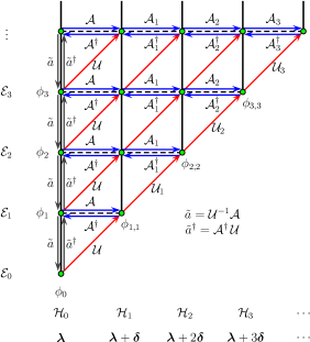
Figure 1: A schematic diagram of the energy levels and the associated Hamiltonian systems together with the definition of the $\mathcal{A}$ and $\mathcal{A}^{\dagger}$ operators and the ‘creation’ ($\tilde{a}^{\dagger}$) and ‘annihilation’ ($\tilde{a}$) operators. The parameter set is indicated below each Hamiltonian.

As seen above, the operators $\mathcal{A}$ and $\mathcal{A}^{\dagger}$ act isospectrally, that is horizontally. On the other hand, the annihilation and creation operators map from one eigenstate to another, i.e. vertically, of a given Hamiltonian. In order to define the annihilation and creation operators, let us introduce normalized basis $\{\hat{\phi}_{s,n}\}_{n\geq s}$ for each Hamiltonian $\mathcal{H}_{s}$ and unitary operators $\mathcal{U}_{s}=\mathcal{U}_{s}(\bm{\lambda})$ mapping the $s$-th orthonormal basis $\{\hat{\phi}_{s,n}\}_{n\geq s}$ to the $(s+1)$-th $\{\hat{\phi}_{s+1,n}\}_{n\geq s+1}$ (see Fig.1 and for example [23, 28]):

$$\mathcal{U}_{s}(\bm{\lambda})\hat{\phi}_{s,n}(y\,;\bm{\lambda})=\hat{\phi}_{s+1,n+1}(y\,;\bm{\lambda}),\quad\mathcal{U}_{s}(\bm{\lambda})^{\dagger}\hat{\phi}_{s+1,n+1}(y\,;\bm{\lambda})=\hat{\phi}_{s,n}(y\,;\bm{\lambda}).$$ (59)

We denote $\mathcal{U}_{0}=\mathcal{U}$. Roughly speaking $\mathcal{U}$ increases the parameters from $\bm{\lambda}$ to $\bm{\lambda}+\bm{\delta}$. Then an annihilation $\tilde{a}$ and a creation operator $\tilde{a}^{\dagger}$ for the Hamiltonian $\mathcal{H}$ are introduced as follows:

$$\tilde{a}=\tilde{a}(y\,;\bm{\lambda})\stackrel{{\scriptstyle\rm def}}{{=}}\mathcal{U}^{\dagger}(\bm{\lambda})\mathcal{A}(y\,;\bm{\lambda}),\quad\tilde{a}^{\dagger}=\tilde{a}(y\,;\bm{\lambda})^{\dagger}\stackrel{{\scriptstyle\rm def}}{{=}}\mathcal{A}(y\,;\bm{\lambda})^{\dagger}\mathcal{U}(\bm{\lambda}).$$ (60)

It is straightforward to derive

$$\mathcal{H}(y\,;\bm{\lambda})=\tilde{a}(y\,;\bm{\lambda})^{\dagger}\tilde{a}(y\,;\bm{\lambda}),$$ (61)

$$\bigl{[}\tilde{a}(y\,;\bm{\lambda}),\tilde{a}(y\,;\bm{\lambda})^{\dagger}\bigr{]}\hat{\phi}_{n}(y\,;\lambda)=({\cal E}_{n+1}(\bm{\lambda})-{\cal E}_{n}(\bm{\lambda}))\hat{\phi}_{n}(y\,;\lambda).$$ (62)

In the present case $U$ is an identity map and we recover the well-known result. This scheme is illustrated in Figure 1.

The above Rodrigues-type formula (56)–(57) gives $\phi_{n}(y)\propto H_{n}(y)\phi_{0}(y)$. This can be also understood in the following manner. By similarity transformation in terms of the ground state wavefunction, let us define $\tilde{\mathcal{H}}$,

$$\tilde{\mathcal{H}} =\phi_{0}(y\,;\bm{\lambda})^{-1}\circ\mathcal{H}\circ\phi_{0}(y\,;\bm{\lambda})=-\frac{1}{2}\frac{d^{2}}{dy^{2}}-\frac{d\,\mathcal{W}(y\,;\bm{\lambda})}{dy}\frac{d}{dy}\,,$$ (63)

$$=BC,\quad B=-i\bigl{(}\tfrac{d}{dy}+2\tfrac{d\,\mathcal{W}(y\,;\bm{\lambda})}{dy}\bigr{)},\quad C=-\tfrac{i}{2}\tfrac{d}{dy},$$ (64)

and consider higher eigenfunctions in a product form $\phi_{n}(y\,;\bm{\lambda})=P_{n}(y\,;\bm{\lambda})\phi_{0}(y\,;\bm{\lambda})$, where $P_{n}(y\,;\bm{\lambda})$ satisfies

$$\tilde{\mathcal{H}}(y\,;\bm{\lambda})P_{n}(y\,;\bm{\lambda})=\mathcal{E}_{n}(\bm{\lambda})P_{n}(y\,;\bm{\lambda}).$$ (65)

In the present case we have

$$\tilde{\mathcal{H}}=-\frac{1}{2}\frac{d^{2}}{dy^{2}}+y\frac{d}{dy}\,.$$ (66)

Since the Hermite polynomial satisfies

$$\Bigl{(}\frac{d^{2}}{dy^{2}}-2y\frac{d}{dy}+2n\Bigr{)}H_{n}(y)=0,$$ (67)

we obtain

$$P_{n}(y)\propto H_{n}(y),\quad\mathcal{E}_{n}=n.$$ (68)

The energy of $H$ is

$$E_{n}=\hbar\omega n\,.$$ (69)

3.2 Ruijsenaars-Schneider-van Diejen Systems

The Hamiltonian is (11) with the potential (13)–(14).

3.2.1 Equilibrium positions of $n$-particle classical systems

Let us consider a polynomial whose zeros give the equilibrium positions, $f(y)=\prod_{j=1}^{n}(y-\sqrt{\frac{m\omega_{1}}{\bar{g}}}\,\bar{q}_{j})$. Then (34) can be converted to a functional equation for $f(y)$. We can show that the solutions of this functional equation satisfy the three-term recurrence which agrees with that of the continuous Hahn polynomials of specific parameters. The result is [12]

$$\prod_{j=1}^{n}\Bigl{(}y-\sqrt{\frac{m\omega_{1}}{\bar{g}}}\,\bar{q}_{j}\Bigr{)}=p_{n}^{\rm monic}\Bigl{(}\sqrt{\frac{mc^{2}}{\omega_{1}\bar{g}}}\,y\,;\frac{mc^{2}}{\omega_{1}\bar{g}},\frac{mc^{2}}{\omega_{2}\bar{g}},\frac{mc^{2}}{\omega_{1}\bar{g}},\frac{mc^{2}}{\omega_{2}\bar{g}}\Bigr{)}\,,$$ (70)

where $p_{n}(y;a_{1},a_{2},b_{1},b_{2})=\frac{1}{n!}(n+a_{1}+a_{2}+b_{1}+b_{2}-1)_{n}\,p_{n}^{\rm monic}(y;a_{1},a_{2},b_{1},b_{2})$ is the continuous Hahn polynomial [18].

3.2.2 Eigenfunctions of single-particle quantum mechanics

Let us consider single-particle case ($n=1$). The potential $V_{1}(q)$ is simply $V_{1}(q)=w(q_{1})$. Let us write $x=q_{1}$. The Hamiltonian (11) becomes

$$H=\frac{mc^{2}}{2}\Bigl{(}\sqrt{w(x)}\,e^{-i\frac{\hbar}{mc}\frac{d}{dx}}\sqrt{w(x)^{*}}+\sqrt{w(x)^{*}}\,e^{i\frac{\hbar}{mc}\frac{d}{dx}}\sqrt{w(x)}-w(x)-w(x)^{*}\Bigr{)}\,.$$ (71)

By introducing a dimensionless variable $y$ and a rescaled potential $V(y)$,

$$y=\frac{mc}{\hbar}x\,,$$ (72)

$$V(y)=V\bigl{(}y\,;(a_{1},a_{2})\bigr{)}=(a_{1}+iy)(a_{2}+iy)\,,$$ (73)

$w(x)$ and $H$ are expressed as

$$w(x)=\frac{\hbar\omega_{1}}{mc^{2}}\frac{\hbar\omega_{2}}{mc^{2}}V\Bigl{(}y\,;\bigl{(}\frac{mc^{2}}{\hbar\omega_{1}},\frac{mc^{2}}{\hbar\omega_{2}}\bigr{)}\Bigr{)}\,,$$ (74)

$$H=mc^{2}\frac{\hbar\omega_{1}}{mc^{2}}\frac{\hbar\omega_{2}}{mc^{2}}\mathcal{H}\,.$$ (75)

Here $\mathcal{H}$ is defined by

$$\mathcal{H}=\frac{1}{2}\Bigl{(}\sqrt{V(y)}\,e^{-i\frac{d}{dy}}\sqrt{V(y)^{*}}+\sqrt{V(y)^{*}}\,e^{i\frac{d}{dy}}\sqrt{V(y)}-V(y)-V(y)^{*}\Bigr{)}\,,$$ (76)

where $V(y)$ is $V(y;\bm{\lambda})$ (73) with $\bm{\lambda}=(a_{1},a_{2})=(\frac{mc^{2}}{\hbar\omega_{1}},\frac{mc^{2}}{\hbar\omega_{2}})$. In the following we will consider arbitrary positive parameters $a_{1}$ and $a_{2}$. Instead of $H\phi_{n}=E_{n}\phi_{n}$, let us consider a rescaled equation $\mathcal{H}\phi_{n}(y)=\mathcal{E}_{n}\phi_{n}(y)$ $(n=0,1,2,\ldots)$, where energies are related as $E_{n}=\frac{\hbar^{2}\omega_{1}\omega_{2}}{mc^{2}}\mathcal{E}_{n}$.

The Hamiltonian $\mathcal{H}$ is factorizable:

$$\mathcal{H} =\mathcal{H}(y\,;\bm{\lambda})=\mathcal{A}(y\,;\bm{\lambda})^{\dagger}\mathcal{A}(y\,;\bm{\lambda})\,,$$ (77)

$$\mathcal{A} =\mathcal{A}(y\,;\bm{\lambda})\stackrel{{\scriptstyle\rm def}}{{=}}\frac{1}{\sqrt{2}}\Bigl{(}e^{-\frac{i}{2}\frac{d}{dy}}\sqrt{V(y\,;\bm{\lambda})^{*}}-e^{\frac{i}{2}\frac{d}{dy}}\sqrt{V(y\,;\bm{\lambda})}\,\Bigr{)}\,,$$ (78)

$$\mathcal{A}^{\dagger} =\mathcal{A}(y\,;\bm{\lambda})^{\dagger}\stackrel{{\scriptstyle\rm def}}{{=}}\frac{1}{\sqrt{2}}\Bigl{(}\sqrt{V(y\,;\bm{\lambda})}\,e^{-\frac{i}{2}\frac{d}{dy}}-\sqrt{V(y\,;\bm{\lambda})^{*}}\,e^{\frac{i}{2}\frac{d}{dy}}\Bigr{)}\,.$$ (79)

The ground state of $\mathcal{H}$ is annihilated by $\mathcal{A}$,

$$\phi_{0}(y\,;\bm{\lambda})\propto\bigl{|}\Gamma(a_{1}+iy)\Gamma(a_{2}+iy)\bigr{|}\,,\quad\mathcal{E}_{0}(\bm{\lambda})=0.$$ (80)

It is easy to verify that the Hamiltonian $\mathcal{H}$ is shape invariant (44) with

$$\bm{\delta}=(\tfrac{1}{2},\tfrac{1}{2})\,,\quad\mathcal{E}_{1}(\bm{\lambda})=a_{1}+a_{2}\,.$$ (81)

Like in §3.1.2, let us define $\mathcal{A}_{s}$, $\mathcal{H}_{s}$ and $\phi_{s,n}$ ($n\geq s\geq 0$) by (46)–(48). Then for $n\geq s\geq 0$ we obtain (49)–(54) and (55)–(57). From (51) and (81) we get

$$\mathcal{E}_{n}(\bm{\lambda})=\tfrac{1}{2}n(n+2a_{1}+2a_{2}-1).$$ (82)

By similarity transformation in terms of the ground state wavefunction, we define $\tilde{\mathcal{H}}$,

$$\tilde{\mathcal{H}} =\phi_{0}(y\,;\bm{\lambda})^{-1}\circ\mathcal{H}\circ\phi_{0}(y\,;\bm{\lambda})=\frac{1}{2}\Bigl{(}V(y)e^{-i\frac{d}{dy}}+V(y)^{*}e^{i\frac{d}{dy}}-V(y)-V(y)^{*}\Bigr{)},$$ (83)

$$=BC,\quad B=-i\bigl{(}V(y)e^{-\frac{i}{2}\frac{d}{dy}}-V(y)^{*}e^{\frac{i}{2}\frac{d}{dy}}\bigr{)},\quad C=\tfrac{i}{2}\bigl{(}e^{-\frac{i}{2}\frac{d}{dy}}-e^{\frac{i}{2}\frac{d}{dy}}\bigr{)},$$ (84)

and consider $\phi_{n}(y\,;\bm{\lambda})=P_{n}(y\,;\bm{\lambda})\phi_{0}(y\,;\bm{\lambda})$, where $P_{n}(y\,;\bm{\lambda})$ satisfies (65). This means that $P_{n}(y\,;\bm{\lambda})$ is a special case of the continuous Hahn polynomial

$$P_{n}(y;\bm{\lambda})\propto p_{n}(y\,;a_{1},a_{2},a_{1},a_{2}),\quad\mathcal{E}_{n}(\bm{\lambda})=\tfrac{1}{2}n(n+2a_{1}+2a_{2}-1).$$ (85)

The energy of $H$ is

$$E_{n}=\hbar(\omega_{1}+\omega_{2})n+\frac{\hbar^{2}\omega_{1}\omega_{2}}{2mc^{2}}n(n-1).$$ (86)

In the $c\rightarrow\infty$ limit we have $\displaystyle\lim_{c\rightarrow\infty}E_{n}=\hbar(\omega_{1}+\omega_{2})n$ and this is consistent with (24), (25) and (69).

4 Rational $BC$ Types

In this section we consider CS and RSvD systems with rational $BC$ type potentials. Relevant polynomials are the Laguerre polynomial and the Wilson polynomial.

4.1 Calogero Systems

The Hamiltonian is (1) with the potential (5)–(6).

4.1.1 Equilibrium positions of $n$-particle classical systems

Let us consider a polynomial whose zeros give the equilibrium positions, $f(y)=\prod_{j=1}^{n}(y^{2}-\frac{m\omega}{\bar{g}_{M}}\,\bar{q}_{j}^{2})$. Then (32) can be converted to a differential equation for $f(y)$, which is the differential equation for the Laguerre polynomial. The result is

$$\prod_{j=1}^{n}\Bigl{(}y^{2}-\frac{m\omega}{\bar{g}_{M}}\,\bar{q}_{j}^{2}\Bigr{)}=L_{n}^{(\alpha)\,{\rm monic}}(y^{2})\,,\quad\alpha=\frac{\bar{g}_{S}+\bar{g}_{L}}{\bar{g}_{M}}-1\,,$$ (87)

where $L_{n}^{(\alpha)}(y^{2})=\frac{(-1)^{n}}{n!}L_{n}^{(\alpha)\,{\rm monic}}(y^{2})$ is the Laguerre polynomial [18].

4.1.2 Eigenfunctions of single-particle quantum mechanics

Let us consider the single-particle case ($n=1$) and write $x=q_{1}$ and $g=g_{S}+g_{L}$. The Hamiltonian (1) describes the harmonic oscillator with a centrifugal barrier and a constant energy shift

$$H=-\frac{\hbar^{2}}{2m}\frac{d^{2}}{dx^{2}}+\frac{1}{2}m\omega^{2}x^{2}+\frac{\hbar^{2}}{2m}\frac{g(g-1)}{x^{2}}-\hbar\omega\Bigl{(}g+\frac{1}{2}\Bigr{)}\,.$$ (88)

By introducing a dimensionless variable $y$ (37), $H$ can be written as

$$H=\hbar\omega\mathcal{H}\,,\quad\mathcal{H}=-\frac{1}{2}\frac{d^{2}}{dy^{2}}+\frac{1}{2}y^{2}+\frac{g(g-1)}{2y^{2}}-g-\frac{1}{2}\,.$$ (89)

This $\mathcal{H}$ has a parameter $g$ and we will write $\bm{\lambda}=g$. Instead of $H\phi_{n}=E_{n}\phi_{n}$, let us consider a rescaled equation $\mathcal{H}\phi_{n}(y)=\mathcal{E}_{n}\phi_{n}(y)$ ($n=0,1,2,\ldots$), where energies are related as $E_{n}=\hbar\omega\mathcal{E}_{n}$.

Like in §3.1.2, $\mathcal{H}$ is factorizable (39)–(41), where the prepotential with parameter $\bm{\lambda}=g$ is

$$\mathcal{W}(y\,;\bm{\lambda})=-\tfrac{1}{2}y^{2}+g\log y.$$ (90)

The ground state wavefunction of $\mathcal{H}$ is (42),

$$\phi_{0}(y\,;\bm{\lambda})\propto y^{g}e^{-\frac{1}{2}y^{2}},\quad\mathcal{E}_{0}(\bm{\lambda})=0.$$ (91)

The Hamiltonian $\mathcal{H}$ is shape invariant (44) with

$$\bm{\delta}=1,\quad\mathcal{E}_{1}(\bm{\lambda})=2.$$ (92)

Let us define $\mathcal{A}_{s}$, $\mathcal{H}_{s}$ and $\phi_{s,n}$ ($n\geq s\geq 0$) by (46)–(48). Then for $n\geq s\geq 0$ we arrive at the consequence of the shape-invariance (49)–(54) and (55)–(57). From (51) and (92) we find the energy spectrum

$$\mathcal{E}_{n}(\bm{\lambda})=2n.$$ (93)

The Rodrigues-type formula (56)–(57) gives $\phi_{n}(y\,;g)\propto L_{n}^{(g-\frac{1}{2})}(y^{2})\phi_{0}(y\,;g)$. This can be also understood as (63)–(65),

$$\tilde{\mathcal{H}}=-\frac{1}{2}\frac{d^{2}}{dy^{2}}+\bigl{(}y-\frac{g}{y}\bigr{)}\frac{d}{dy}=2\Bigl{(}-\eta\frac{d^{2}}{d\eta^{2}}+(\eta-g-\tfrac{1}{2})\frac{d}{d\eta}\Bigr{)}\,,\quad(\eta=y^{2}).$$ (94)

Since the Laguerre polynomial satisfies

$$\Bigl{(}\eta\frac{d^{2}}{d\eta^{2}}+(\alpha+1-\eta)\frac{d}{d\eta}+n\Bigr{)}L_{n}^{(\alpha)}(\eta)=0,$$ (95)

we obtain

$$P_{n}(y\,;g)\propto L_{n}^{(g-\frac{1}{2})}(y^{2}),\quad\mathcal{E}_{n}(g)=2n.$$ (96)

The energy of $H$ is

$$E_{n}(g)=\hbar\omega 2n.$$ (97)

Remark: For the given potential $V_{\rm CS}(x)$, the prepotential $W(x)$ is obtained by solving the Riccati equation $V_{\rm CS}(x)=\frac{1}{2m}(W^{\prime}(x)^{2}+\hbar W^{\prime\prime}(x))+\text{constant}$. The above prepotential (90) is one solution. Since the Hamiltonian(except for the constant term) contains $g$ as the combination $g(g-1)$, we have another solution $\check{\mathcal{W}}$,

$$\check{\mathcal{W}}(y\,;g)=\mathcal{W}(y\,;1-g),$$ (98)

and the corresponding Hamiltonian $\check{\mathcal{H}}$ is

$$\check{\mathcal{H}}(y\,;g)=\check{\mathcal{A}}(y\,;g)^{\dagger}\check{\mathcal{A}}(y\,;g)=\mathcal{H}(y\,;g)+2g-1.$$ (99)

The ground state wavefunction of $\check{\mathcal{H}}$ (the state annihilated by $\check{\mathcal{A}}(y\,;g)$) is

$$\check{\phi}_{0}(y\,;g)\propto e^{\check{\mathcal{W}}(y\,;g)}=y^{1-g}e^{-\frac{1}{2}y^{2}},\quad\check{\mathcal{E}}_{0}(g)=0,$$ (100)

which is square integrable for $g<\frac{3}{2}$. Note that $\phi_{0}(y\,;g)$ (91) is square integrable for $g>-\frac{1}{2}$. These two ‘ground’ states define two sectors of this system. Usually we consider only one of them. Note that $\mathcal{A}(y\,;g)\check{\phi}_{0}(y\,;g)$ is square integrable for $g\leq\frac{1}{2}$. From the Rodrigues-type formula and the recurrence relation of the energy, we obtain

$$\check{\phi}_{n}(y\,;g)\propto L_{n}^{(\frac{1}{2}-g)}(y^{2})\check{\phi}_{0}(y\,;g),\quad\check{\mathcal{E}}_{n}(g)=2n.$$ (101)

The corresponding energy of $H$ is

$$\check{E}_{n}(g)=\hbar\omega(2n+1-2g).$$ (102)

Therefore, for $g<\frac{3}{2}$ ($g\neq\frac{1}{2}$), we have another sector of the system, (101) with (102). The order of $E_{n}(g)$ (97) and $\check{E}_{n}(g)$ (102) is

$$E_{0}(g)<\check{E}_{0}(g)<E_{1}(g)<\check{E}_{1}(g)<E_{2}(g)<\check{E}_{2}(g)<\cdots\quad \text{ for }-\tfrac{1}{2}<g<\tfrac{1}{2}\,,$$ (103)

$$\check{E}_{0}(g)<E_{0}(g)<\check{E}_{1}(g)<E_{1}(g)<\check{E}_{2}(g)<E_{2}(g)<\cdots\quad \text{ for }\quad\ \tfrac{1}{2}<g<\tfrac{3}{2}\,.$$ (104)

Thus the lowest energy state of $H$ is $\phi_{0}(y\,;g)$ for $g\geq\frac{3}{2}$ or $-\frac{1}{2}<g\leq\frac{1}{2}$ (which cover all values of $g(g-1)\geq-\frac{1}{4}$), and $\check{\phi}_{0}(y\,;g)$ for $\frac{1}{2}<g<\frac{3}{2}$. In the $g\rightarrow 0$(or 1) limit, both sectors contribute and these eigenfunctions reduce to those in §3.1.2 due to the identities,

$$\phi_{n}(y\,;g\rightarrow 0)\propto L_{n}^{(-\frac{1}{2})}(y^{2})\,e^{-\frac{1}{2}y^{2}}\propto H_{2n}(y)\,e^{-\frac{1}{2}y^{2}},$$ (105)

$$\check{\phi}_{n}(y\,;g\rightarrow 0)\propto L_{n}^{(\frac{1}{2})}(y^{2})\,y\,e^{-\frac{1}{2}y^{2}}\propto H_{2n+1}(y)\,e^{-\frac{1}{2}y^{2}}.$$ (106)

4.2 Ruijsenaars-Schneider-van Diejen Systems

The Hamiltonian is (11) with the potential (15)–(16).

4.2.1 Equilibrium positions of $n$-particle classical systems

Let us consider a polynomial whose zeros give the equilibrium positions, $f(y)=\prod_{j=1}^{n}(y^{2}-\frac{m\omega_{1}}{\bar{g}_{0}}\,\bar{q}_{j}^{2})$. Then (34) can be converted to a functional equation for $f(y)$. We can show that the solutions of this functional equation satisfy the three-term recurrence which agrees with that of the Wilson polynomials. The result is [12]

$$\prod_{j=1}^{n}\Bigl{(}y^{2}-\frac{m\omega_{1}}{\bar{g}_{0}}\,\bar{q}_{j}^{2}\Bigr{)}=W_{n}^{\rm monic}\Bigl{(}\frac{mc^{2}}{\omega_{1}\bar{g}_{0}}\,y^{2};\frac{mc^{2}}{\omega_{1}\bar{g}_{0}},\frac{mc^{2}}{\omega_{2}\bar{g}_{0}},\frac{\bar{g}_{1}}{\bar{g}_{0}},\frac{\bar{g}_{2}}{\bar{g}_{0}}\Bigr{)}\,,$$ (107)

where $W_{n}(y^{2};a_{1},a_{2},a_{3},a_{4})=(-1)^{n}(n+a_{1}+a_{2}+a_{3}+a_{4}-1)_{n}\,W_{n}^{\rm monic}(y^{2};a_{1},a_{2},a_{3},a_{4})$ is the Wilson polynomial [18].

4.2.2 Eigenfunctions of single-particle quantum mechanics

Let us consider the single-particle case ($n=1$). The potential $V_{1}(q)$ is $V_{1}(q)=w(q_{1})$. Let us write $x=q_{1}$. The Hamiltonian (11) becomes (71) with $w(x)$ in (16). By introducing a dimensionless variable $y$ (72) and a rescaled potential $V(y)$,

$$V(y)=V\bigl{(}y\,;(a_{1},a_{2},a_{3},a_{4})\bigr{)}=\frac{(a_{1}+iy)(a_{2}+iy)(a_{3}+iy)(a_{4}+iy)}{2iy(2iy+1)}\,,$$ (108)

$w(x)$ and $H$ are expressed as

$$w(x)=4\frac{\hbar\omega_{1}}{mc^{2}}\frac{\hbar\omega_{2}}{mc^{2}}V\Bigl{(}y\,;\bigl{(}\frac{mc^{2}}{\hbar\omega_{1}},\frac{mc^{2}}{\hbar\omega_{2}},g_{1},g_{2}\bigr{)}\Bigr{)}\,,$$ (109)

$$H=4mc^{2}\frac{\hbar\omega_{1}}{mc^{2}}\frac{\hbar\omega_{2}}{mc^{2}}\mathcal{H}\,.$$ (110)

Here rescaled Hamiltonian $\mathcal{H}$ is defined by (76), where $V(y)$ is $V(y;\bm{\lambda})$ (108) with $\bm{\lambda}=(a_{1},a_{2},a_{3},a_{4})=(\frac{mc^{2}}{\hbar\omega_{1}},\frac{mc^{2}}{\hbar\omega_{2}},g_{1},g_{2})$. In the following we will consider arbitrary positive parameters $a_{1},a_{2},a_{3},a_{4}$. Instead of $H\phi_{n}=E_{n}\phi_{n}$, let us consider the rescaled equation $\mathcal{H}\phi_{n}(y)=\mathcal{E}_{n}\phi_{n}(y)$ $(n=0,1,2,\ldots)$, where energies are related as $E_{n}=\frac{4\hbar^{2}\omega_{1}\omega_{2}}{mc^{2}}\mathcal{E}_{n}$.

Like in §3.2.2, $\mathcal{H}$ is factorizable (77)–(79). The ground state of $\mathcal{H}$ is annihilated by $\mathcal{A}$,

$$\phi_{0}(y\,;\lambda)\propto\biggl{|}\frac{\Gamma(a_{1}+iy)\Gamma(a_{2}+iy)\Gamma(a_{3}+iy)\Gamma(a_{4}+iy)}{\Gamma(2iy)}\biggr{|}\,.$$ (111)

The Hamiltonian $\mathcal{H}$ is shape invariant (44) with

$$\bm{\delta}=(\tfrac{1}{2},\tfrac{1}{2},\tfrac{1}{2},\tfrac{1}{2}),\quad\mathcal{E}_{1}(\bm{\lambda})=\tfrac{1}{2}(a_{1}+a_{2}+a_{3}+a_{4}).$$ (112)

The third and fourth components of $\bm{\delta}$ are consistent with $\bm{\delta}$ in (92) because of (24) and (26). Let us define $\mathcal{A}_{s}$, $\mathcal{H}_{s}$ and $\phi_{s,n}$ ($n\geq s\geq 0$) by (46)–(48). Then for $n\geq s\geq 0$ we obtain the consequences of the shape-invariance (49)–(54) and (55)–(57). From (51) and (112) we obtain the energy spectrum

$$\mathcal{E}_{n}(\bm{\lambda})=\frac{1}{2}n(n+a_{1}+a_{2}+a_{3}+a_{4}-1).$$ (113)

By similarity transformation in terms of the ground state wavefunction, (83)–(84) and (65) imply that $P_{n}(y\,;\bm{\lambda})$ is the Wilson polynomial

$$P_{n}(y\,;\bm{\lambda})\propto W_{n}(y^{2};\bm{\lambda}),\quad\mathcal{E}_{n}(\bm{\lambda})=\frac{1}{2}n(n+a_{1}+a_{2}+a_{3}+a_{4}-1).$$ (114)

The energy of $H$ is

$$E_{n}=\hbar(\omega_{1}+\omega_{2})2n+\frac{\hbar^{2}\omega_{1}\omega_{2}}{mc^{2}}2n(n+g_{1}+g_{2}-1).$$ (115)

In the $c\rightarrow\infty$ limit we have $\displaystyle\lim_{c\rightarrow\infty}E_{n}=\hbar(\omega_{1}+\omega_{2})2n$ and this is consistent with (24), (26) and (97).

5 Trigonometric $A$ Types

In this section we consider the CS and RSvD systems with the trigonometric $A$ type potentials. The single-particle quantum mechanics is free theory and cosine (or sine) functions are the eigenfunctions.

5.1 Sutherland Systems

The Hamiltonian is (1) with the potential (7)–(8).

5.1.1 Equilibrium positions of $n$-particle classical systems

The equation for the equilibrium positions (32) is easily solved,

$$\frac{\pi}{L}\bar{q}_{j}=\frac{\pi}{n}(n+1-j)+\alpha\qquad(j=1,\ldots,n),$$ (116)

where $\alpha$ is an arbitrary real number which is a consequence of the translational invariance. The rescaled equilibrium positions $\frac{\pi}{L}\bar{q}_{j}$ are zeros of $\cos n(\theta-\alpha^{\prime})$ ($\alpha^{\prime}=\alpha-\frac{\pi}{2n}$), which is equal to

$$T_{n}\bigl{(}\cos(\theta-\alpha^{\prime})\bigr{)}.$$ (117)

Here $T_{n}(\cos\varphi)=\cos n\varphi$ is the Chebyshev polynomial of the first kind [18].

5.1.2 Eigenfunctions of single-particle quantum mechanics

Let us consider the single-particle case ($n=1$) and write $x=q_{1}$. We impose the periodic boundary condition on the wave function $\phi(x)$, $\phi(x+L)=\phi(x)$. The Hamiltonian (11) is a free one

$$H=-\frac{\hbar^{2}}{2m}\frac{d^{2}}{dx^{2}}.$$ (118)

By introducing a dimensionless variable $y$,

$$y=\frac{\pi}{L}x,$$ (119)

$H$ can be written as

$$H=\frac{\hbar^{2}\pi^{2}}{mL^{2}}\mathcal{H}\,,\quad\mathcal{H}=-\frac{1}{2}\frac{d^{2}}{dy^{2}}\,.$$ (120)

Moreover in terms of another dimensionless variable $z$,

$$z=e^{2iy}=e^{2\pi i\frac{x}{L}},$$ (121)

$\mathcal{H}$ becomes

$$\mathcal{H}=2D_{z}^{2}\,,\quad D_{z}\stackrel{{\scriptstyle\rm def}}{{=}}z\frac{d}{dz}\,.$$ (122)

The eigenfunctions of $\mathcal{H}$ (with periodic boundary condition in $x$) are easily obtained: $z^{n}$ ($n\in\mathbb{Z}$). Except for the ground state, eigenstates are doubly degenerated,

$$\phi_{0}(z)\propto 1,\quad\phi_{n}(z)\propto c_{1}z^{n}+c_{2}z^{-n}\propto\cos n(2y-\alpha^{\prime})=T_{n}(\cos(2y-\alpha^{\prime}))\quad(n\geq 1),$$ (123)

$$\mathcal{E}_{n}=2n^{2}\quad(n\geq 0),$$ (124)

where $c_{1},c_{2},\alpha^{\prime}$ are arbitrary numbers. The variable $2y$ should be identified with $\theta$ in §5.1.1 (see §6.1.2). The energy spectrum of $H$ is

$$E_{n}=\frac{\hbar^{2}\pi^{2}}{mL^{2}}2n^{2}\,.$$ (125)

5.2 Ruijsenaars-Schneider Systems

The Hamiltonian is (11) with the potential (17)–(18).

5.2.1 Equilibrium positions of $n$-particle classical systems

The equation for the equilibrium positions (33) is easily solved and the equilibrium positions are the same as those given in §5.1.1, (116).

5.2.2 Eigenfunctions of single-particle quantum mechanics

Let us consider the single-particle case ($n=1$). The potential $V_{1}(q)$ is trivial $V_{1}(q)=w(q_{1})=1$. Let us write $x=q_{1}$. We impose the periodic boundary condition $\phi(x+L)=\phi(x)$, too. The Hamiltonian (11) becomes

$$H=\frac{mc^{2}}{2}\bigl{(}e^{-i\frac{\hbar}{mc}\frac{d}{dx}}+e^{i\frac{\hbar}{mc}\frac{d}{dx}}-2\bigr{)}\,.$$ (126)

By introducing a dimensionless variable $y$ (119) and $z$ (121), $H$ can be written as

$$H=mc^{2}\mathcal{H}\,,\quad\mathcal{H}=\tfrac{1}{2}\bigl{(}e^{-i\frac{d}{dy}}+e^{i\frac{d}{dy}}-2\bigr{)}=\tfrac{1}{2}\bigl{(}q^{-D_{z}}+q^{D_{z}}-2\bigr{)},$$ (127)

where we have introduced a dimensionless parameter $q$,

$$q=e^{-\frac{2\pi\hbar}{mcL}},\quad 0<q<1.$$ (128)

The operator $q^{D_{z}}$ causes a $q$-shift, $q^{D_{z}}f(z)=f(qz)$. Again this is a free theory and the eigenfunctions of $\mathcal{H}$ (with periodic boundary condition in $x$) are easily obtained: $z^{n}$ ($n\in\mathbb{Z}$). Except for the ground state, eigenstates are doubly degenerate: (123) and

$$\mathcal{E}_{n}=2\sinh^{2}\frac{\hbar\pi n}{mcL}\quad(n\geq 0).$$ (129)

The energy spectrum of $H$ is

$$E_{n}=2mc^{2}\sinh^{2}\frac{\hbar\pi n}{mcL}\,.$$ (130)

In the $c\rightarrow\infty$ limit we have $\displaystyle\lim_{c\rightarrow\infty}E_{n}=\tfrac{\hbar^{2}\pi^{2}}{mL^{2}}2n^{2}$ and this is consistent with (24), (27) and (125).

6 Trigonometric $BC$ Types

In this section we consider the CS and RSvD systems with the trigonometric $BC$ type potentials. The Jacobi polynomial and the Askey-Wilson polynomial play the role.

6.1 Sutherland Systems

The Hamiltonian is (1) with the potential (9)–(10).

6.1.1 Equilibrium positions of $n$-particle classical systems

Let us consider a polynomial whose zeros give the equilibrium positions, $f(\xi)=\prod_{j=1}^{n}\Bigl{(}\xi-\cos\bigl{(}2\tfrac{\pi}{L}\bar{q}_{j}\bigr{)}\Bigr{)}$. Then (32) can be converted to a differential equation for $f(y)$, which determines the Jacobi polynomial. The result is

$$\prod_{j=1}^{n}\Bigl{(}\xi-\cos\bigl{(}2\tfrac{\pi}{L}\bar{q}_{j}\bigr{)}\Bigr{)}=P_{n}^{(\alpha,\beta)\,{\rm monic}}(\xi)\,,\quad\alpha=\frac{\bar{g}_{S}+\bar{g}_{L}}{\bar{g}_{M}}-1\,,\ \beta=\frac{\bar{g}_{L}}{\bar{g}_{M}}-1\,,$$ (131)

where $P_{n}^{(\alpha,\beta)}(\xi)=2^{-n}\binom{\alpha+\beta+2n}{n}P_{n}^{(\alpha,\beta)\,{\rm monic}}(\xi)$ is the Jacobi polynomial [18].

6.1.2 Eigenfunctions of single-particle quantum mechanics

Let us consider the single-particle case ($n=1$) and write $x=q_{1}$ and $g=g_{S}+g_{L}$, $g^{\prime}=g_{L}$. The Hamiltonian (1) has the Pöschl-Teller potential [29] with a constant energy shift

$$H=-\frac{\hbar^{2}}{2m}\frac{d^{2}}{dx^{2}}+\frac{\hbar^{2}\pi^{2}}{2mL^{2}}\Bigl{(}\frac{g(g-1)}{\sin^{2}\frac{\pi}{L}x}+\frac{g^{\prime}(g^{\prime}-1)}{\cos^{2}\frac{\pi}{L}x}\Bigr{)}-\frac{\hbar^{2}\pi^{2}}{2mL^{2}}(g+g^{\prime})^{2}\,.$$ (132)

By introducing a dimensionless variable $y$ (119), $H$ can be written as

$$H=\frac{\hbar^{2}\pi^{2}}{mL^{2}}\,\mathcal{H}\,,\quad\mathcal{H}=\frac{1}{2}\Bigl{(}-\frac{d^{2}}{dy^{2}}+\frac{g(g-1)}{\sin^{2}y}+\frac{g^{\prime}(g^{\prime}-1)}{\cos^{2}y}-(g+g^{\prime})^{2}\Bigr{)}\,.$$ (133)

This $\mathcal{H}$ has parameters $g$ and $g^{\prime}$ and we will denote $\bm{\lambda}=(g,g^{\prime})$. In the following we will consider arbitrary positive parameters $g$ and $g^{\prime}$. Instead of $H\phi_{n}=E_{n}\phi_{n}$, let us consider $\mathcal{H}\phi_{n}(y)=\mathcal{E}_{n}\phi_{n}(y)$ ($n=0,1,2,\ldots$), where energies are related as $E_{n}=\frac{\hbar^{2}\pi^{2}}{mL^{2}}\mathcal{E}_{n}$.

Like in §3.1.2, $\mathcal{H}$ is factorizable (39)–(41), where the prepotential with parameters $\bm{\lambda}=(g,g^{\prime})$ is

$$\mathcal{W}(y\,;\bm{\lambda})=g\log\sin y+g^{\prime}\log\cos y.$$ (134)

The ground state wavefunction of $\mathcal{H}$ is (42),

$$\phi_{0}(y\,;\bm{\lambda})\propto(\sin y)^{g}(\cos y)^{g^{\prime}},\quad\mathcal{E}_{0}(\bm{\lambda})=0.$$ (135)

The Hamiltonian $\mathcal{H}$ is shape invariant (44) with

$$\bm{\delta}=(1,1),\quad\mathcal{E}_{1}(\bm{\lambda})=2(g+g^{\prime}+1).$$ (136)

Let us define $\mathcal{A}_{s}$, $\mathcal{H}_{s}$ and $\phi_{s,n}$ ($n\geq s\geq 0$) by (46)–(48). Then for $n\geq s\geq 0$ we obtain the consequence of the shape-invariance (49)–(54) and (55)–(57). From (51) and (136) we obtain

$$\mathcal{E}_{n}(\bm{\lambda})=2n(n+g+g^{\prime}).$$ (137)

The Rodrigues-type formula (56)–(57) gives $\phi_{n}(y)\propto P_{n}^{(g-\frac{1}{2},g^{\prime}-\frac{1}{2})}(\cos 2y)\phi_{0}(y)$. This can be also understood as (63)–(65),

$$\tilde{\mathcal{H}} =-\frac{1}{2}\frac{d^{2}}{dy^{2}}-\bigl{(}g\cot y-g^{\prime}\tan y\bigr{)}\frac{d}{dy}$$

$$=-2\Bigl{(}(1-\xi^{2})\frac{d^{2}}{d\xi^{2}}-\bigl{(}g-g^{\prime}+(g+g^{\prime}+1)\xi\bigr{)}\frac{d}{d\xi}\Bigr{)}\,,\quad(\xi={\rm Re}z=\cos 2y).$$ (138)

Since the Jacobi polynomial satisfies

$$\Bigl{(}(1-\xi^{2})\frac{d^{2}}{d\xi^{2}}-\bigl{(}\alpha-\beta+(\alpha+\beta+2)\xi\bigr{)}\frac{d}{d\xi}+n(n+\alpha+\beta+1)\Bigr{)}P_{n}^{(\alpha,\beta)}(\xi)=0,$$ (139)

we obtain

$$P_{n}(z\,;\bm{\lambda})\propto P_{n}^{(g-\frac{1}{2},g^{\prime}-\frac{1}{2})}(\xi),\quad\mathcal{E}_{n}(\bm{\lambda})=2n(n+g+g^{\prime}).$$ (140)

The energy spectrum of $H$ is

$$E_{n}(\bm{\lambda})=\frac{\hbar^{2}\pi^{2}}{mL^{2}}2n(n+g+g^{\prime})=\frac{\hbar^{2}\pi^{2}}{2mL^{2}}\Bigl{(}(2n+g+g^{\prime})^{2}-(g+g^{\prime})^{2}\Bigr{)}.$$ (141)

Remark: Similarly to Remark in §4.1.2, we have three other prepotentials $\check{\mathcal{W}}^{[1]}$, $\check{\mathcal{W}}^{[2]}$, $\check{\mathcal{W}}^{[3]}$,

$$\check{\mathcal{W}}^{[1]}\bigl{(}y\,;(g,g^{\prime})\bigr{)} =\mathcal{W}\bigl{(}y\,;(1-g,g^{\prime})\bigr{)},$$

$$\check{\mathcal{W}}^{[2]}\bigl{(}y\,;(g,g^{\prime})\bigr{)} =\mathcal{W}\bigl{(}y\,;(g,1-g^{\prime})\bigr{)},$$ (142)

$$\check{\mathcal{W}}^{[3]}\bigl{(}y\,;(g,g^{\prime})\bigr{)} =\mathcal{W}\bigl{(}y\,;(1-g,1-g^{\prime})\bigr{)},$$

together with the corresponding Hamiltonians $\check{\mathcal{H}}$:

$$\check{\mathcal{H}}^{[1]}(y\,;\bm{\lambda}) =\check{\mathcal{A}}^{[1]}(y\,;\bm{\lambda})^{\dagger}\check{\mathcal{A}}^{[1]}(y\,;\bm{\lambda})=\mathcal{H}(y\,;\bm{\lambda})+2(g-\tfrac{1}{2})(g^{\prime}+\tfrac{1}{2}),$$

$$\check{\mathcal{H}}^{[2]}(y\,;\bm{\lambda}) =\check{\mathcal{A}}^{[2]}(y\,;\bm{\lambda})^{\dagger}\check{\mathcal{A}}^{[2]}(y\,;\bm{\lambda})=\mathcal{H}(y\,;\bm{\lambda})+2(g+\tfrac{1}{2})(g^{\prime}-\tfrac{1}{2}),$$ (143)

$$\check{\mathcal{H}}^{[3]}(y\,;\bm{\lambda}) =\check{\mathcal{A}}^{[3]}(y\,;\bm{\lambda})^{\dagger}\check{\mathcal{A}}^{[3]}(y\,;\bm{\lambda})=\mathcal{H}(y\,;\bm{\lambda})+2(g+g^{\prime}-1).$$

The ‘ground’ state of $\check{\mathcal{H}}^{[a]}$ ($a=1,2,3$) is $\check{\phi}^{[a]}_{0}(y\,;\bm{\lambda})\propto e^{\check{\mathcal{W}}^{[a]}(y\,;\bm{\lambda})}$ and they are square integrable for $g<\frac{3}{2}$ and/or $g^{\prime}<\frac{3}{2}$. Note that $\phi_{0}(y\,;\bm{\lambda})$ (135) is square integrable for $g,g^{\prime}>-\frac{1}{2}$. These four ‘ground’ states define four sectors of this system. Usually we consider only one of them. Note that $\mathcal{A}(y\,;g)\check{\phi}^{[a]}_{0}(y\,;g)$ is square integrable for $g\leq\frac{1}{2}$ and/or $g^{\prime}\leq\frac{1}{2}$. From the Rodrigues-type formula and the recurrence relation of the energy, we obtain

$$\check{\phi}^{[1]}_{n}(y\,;\bm{\lambda})\propto P_{n}^{(\frac{1}{2}-g,g^{\prime}-\frac{1}{2})}(\cos 2y)\check{\phi}^{[1]}_{0}(y\,;\bm{\lambda}),\quad\check{\mathcal{E}}^{[1]}_{n}(\bm{\lambda})=2n(n+1-g+g^{\prime}),$$

$$\check{\phi}^{[2]}_{n}(y\,;\bm{\lambda})\propto P_{n}^{(g-\frac{1}{2},\frac{1}{2}-g^{\prime})}(\cos 2y)\check{\phi}^{[2]}_{0}(y\,;\bm{\lambda}),\quad\check{\mathcal{E}}^{[2]}_{n}(\bm{\lambda})=2n(n+1+g-g^{\prime}),$$ (144)

$$\check{\phi}^{[3]}_{n}(y\,;\bm{\lambda})\propto P_{n}^{(\frac{1}{2}-g,\frac{1}{2}-g^{\prime})}(\cos 2y)\check{\phi}^{[3]}_{0}(y\,;\bm{\lambda}),\quad\check{\mathcal{E}}^{[3]}_{n}(\bm{\lambda})=2n(n+2-g-g^{\prime}).$$

The corresponding energy spectra of $H$ are

$$\check{E}^{[1]}_{n}(\bm{\lambda}) =\frac{\hbar^{2}\pi^{2}}{2mL^{2}}\Bigl{(}(2n+1-g+g^{\prime})^{2}-(g+g^{\prime})^{2}\Bigr{)},$$

$$\check{E}^{[2]}_{n}(\bm{\lambda}) =\frac{\hbar^{2}\pi^{2}}{2mL^{2}}\Bigl{(}(2n+1+g-g^{\prime})^{2}-(g+g^{\prime})^{2}\Bigr{)},$$ (145)

$$\check{E}^{[3]}_{n}(\bm{\lambda}) =\frac{\hbar^{2}\pi^{2}}{2mL^{2}}\Bigl{(}(2n+2-g-g^{\prime})^{2}-(g+g^{\prime})^{2}\Bigr{)}.$$

Therefore, for $g<\frac{3}{2}$ and/or $g^{\prime}<\frac{3}{2}$, we have these sectors. $\phi_{0}(y\,;\bm{\lambda})$ is the lowest energy state of $H$ for $g,g^{\prime}\geq\frac{3}{2}$ or $-\frac{1}{2}<g,g^{\prime}\leq\frac{1}{2}$. In the $g,g^{\prime}\rightarrow 0$ (or 1) limit, all of these sectors contribute and these eigenfunctions reduce to those in §5.1.2 due to the identities,

$$\phi_{n}\bigl{(}y\,;(g\rightarrow 0,g^{\prime}\rightarrow 0)\bigr{)} \propto P_{n}^{(-\frac{1}{2},-\frac{1}{2})}(\cos 2y)\propto\cos 2ny,$$ (146)

$$\check{\phi}^{[1]}_{n}\bigl{(}y\,;(g\rightarrow 0,g^{\prime}\rightarrow 0)\bigr{)} \propto P_{n}^{(\frac{1}{2},-\frac{1}{2})}(\cos 2y)\sin y\propto\sin(2n+1)y,$$ (147)

$$\check{\phi}^{[2]}_{n}\bigl{(}y\,;(g\rightarrow 0,g^{\prime}\rightarrow 0)\bigr{)} \propto P_{n}^{(-\frac{1}{2},\frac{1}{2})}(\cos 2y)\cos y\propto\cos(2n+1)y,$$ (148)

$$\check{\phi}^{[3]}_{n}\bigl{(}y\,;(g\rightarrow 0,g^{\prime}\rightarrow 0)\bigr{)} \propto P_{n}^{(\frac{1}{2},\frac{1}{2})}(\cos 2y)\sin y\cos y\propto\sin 2(n+1)y.$$ (149)

(The two sets (147) and (148) are excluded by the periodic boundary condition in $x$.)

6.2 Ruijsenaars-Schneider-van Diejen Systems

The Hamiltonian is (11) with the potential (19)–(20).

6.2.1 Equilibrium positions of $n$-particle classical systems

Let us consider a polynomial whose zeros give the equilibrium positions, $f(\xi)=\prod_{j=1}^{n}\Bigl{(}\xi-\cos\bigl{(}2\tfrac{\pi}{L}\bar{q}_{j}\bigr{)}\Bigr{)}$. Then (34) can be converted to a functional equation for $f(y)$. We can show that the solutions of this functional equation satisfy the three-term recurrence which agrees with that of the Wilson polynomials. The result is [12, 15, 13](see also [16])

$$\prod_{j=1}^{n}\Bigl{(}\xi-\cos\bigl{(}2\tfrac{\pi}{L}\bar{q}_{j}\bigr{)}\Bigr{)}=p_{n}^{\rm monic}\bigl{(}\xi\,;e^{-\frac{2\pi\bar{g}_{1}}{mcL}},e^{-\frac{2\pi\bar{g}_{2}}{mcL}},-e^{-\frac{2\pi\bar{g}^{\prime}_{1}}{mcL}},-e^{-\frac{2\pi\bar{g}^{\prime}_{2}}{mcL}}\bigm{|}e^{-\frac{2\pi\bar{g}_{0}}{mcL}}\bigr{)},$$ (150)

where $p_{n}(\xi\,;a_{1},a_{2},a_{3},a_{4}|q)=2^{n}(a_{1}a_{2}a_{3}a_{4}q^{n-1};q)_{n}\,p_{n}^{\rm monic}(\xi\,;a_{1},a_{2},a_{3},a_{4}|q)$ is the Askey - Wilson polynomial [18]. Note that $e^{-\frac{2\pi\bar{g}_{0}}{mcL}}$ etc. are formally expressed as $e^{-\frac{2\pi\hbar g_{0}}{mcL}}=q^{g_{0}}$ etc. by using $q$ in (128).

6.2.2 Eigenfunctions of single-particle quantum mechanics

Let us consider the single-particle case ($n=1$). The potential $V_{1}(q)$ is $V_{1}(q)=w(q_{1})$. Let us write $x=q_{1}$. The Hamiltonian (11) becomes (71) with $w(x)$ in (20). By using $y$ (119), discussion goes parallel to that in §4.2.2, but the variable $z$ (121) is more suitable. So we will reformulate by using $z$ and $q$ (128). By introducing a dimensionless variable $z$ (121) and a rescaled potential $V(z)$,

$$V\bigl{(}z\,;(a_{1},a_{2},a_{3},a_{4}),q\bigr{)}=\frac{(1-a_{1}z)(1-a_{2}z)(1-a_{3}z)(1-a_{4}z)}{(1-z^{2})(1-qz^{2})}\,,$$ (151)

$w(x)$ and $H$ are expressed as

$$w(x)^{*}=q^{-\frac{1}{2}(g_{1}+g_{2}+g^{\prime}_{1}+g^{\prime}_{2})}V(z\,;(q^{g_{1}},q^{g_{2}+\frac{1}{2}},-q^{g^{\prime}_{1}},-q^{g^{\prime}_{2}+\frac{1}{2}}),q),$$ (152)

$$H=mc^{2}q^{-\frac{1}{2}(g_{1}+g_{2}+g^{\prime}_{1}+g^{\prime}_{2})}\mathcal{H}.$$ (153)

Here $\mathcal{H}$ is defined by

$$\mathcal{H}=\frac{1}{2}\Bigl{(}\sqrt{V(z)}\,q^{D_{z}}\sqrt{V(z)^{*}}+\sqrt{V(z)^{*}}\,q^{-D_{z}}\sqrt{V(z)}-V(z)-V(z)^{*}\Bigr{)}\,,$$ (154)

where $V(z)$ is $V(z;\bm{\lambda},q)$ (151) with $\bm{\lambda}=(a_{1},a_{2},a_{3},a_{4})=(q^{g_{1}},q^{g_{2}+\frac{1}{2}},-q^{g^{\prime}_{1}},-q^{g^{\prime}_{2}+\frac{1}{2}})$. In the following we will consider the parameters in the range $-1<a_{1},a_{2},a_{3},a_{4}<1$ and $0<q<1$. Instead of $H\phi_{n}=E_{n}\phi_{n}$, let us consider the rescaled equation $\mathcal{H}\phi_{n}(z)=\mathcal{E}_{n}\phi_{n}(z)$ $(n=0,1,2,\ldots)$, where energies are related as $E_{n}=mc^{2}q^{-\frac{1}{2}(g_{1}+g_{2}+g^{\prime}_{1}+g^{\prime}_{2})}\mathcal{E}_{n}$.

Like in §4.2.2, $\mathcal{H}$ is factorizable:

$$\mathcal{H} =\mathcal{H}(z\,;\bm{\lambda},q)=\mathcal{A}(z\,;\bm{\lambda},q)^{\dagger}\mathcal{A}(z\,;\bm{\lambda},q)\,,$$ (155)

$$\mathcal{A} =\mathcal{A}(z\,;\bm{\lambda},q)\stackrel{{\scriptstyle\rm def}}{{=}}\frac{1}{\sqrt{2}}\Bigl{(}q^{\frac{1}{2}D_{z}}\sqrt{V(z\,;\bm{\lambda},q)^{*}}-q^{-\frac{1}{2}D_{z}}\sqrt{V(z\,;\bm{\lambda},q)}\,\Bigr{)}\,,$$ (156)

$$\mathcal{A}^{\dagger} =\mathcal{A}(z\,;\bm{\lambda},q)^{\dagger}\stackrel{{\scriptstyle\rm def}}{{=}}\frac{1}{\sqrt{2}}\Bigl{(}\sqrt{V(z\,;\bm{\lambda},q)}\,q^{\frac{1}{2}D_{z}}-\sqrt{V(z\,;\bm{\lambda},q)^{*}}\,q^{-\frac{1}{2}D_{z}}\Bigr{)}\,.$$ (157)

The ground state of $\mathcal{H}$ is annihilated by $\mathcal{A}$,

$$\phi_{0}(z)\propto\biggl{|}\frac{(z^{2};q)_{\infty}}{(a_{1}z,a_{2}z,a_{3}z,a_{4}z;q)_{\infty}}\biggr{|}\,.$$ (158)

The Hamiltonian $\mathcal{H}$ is shape invariant but slightly different from the previous form (44)

$$\mathcal{A}(z\,;\bm{\lambda},q)\mathcal{A}(z\,;\bm{\lambda},q)^{\dagger}=q^{2\delta^{\prime}}\mathcal{A}(z\,;q^{\delta}\bm{\lambda},q)^{\dagger}\mathcal{A}(z\,;q^{\delta}\bm{\lambda},q)+\mathcal{E}_{1}(\bm{\lambda},q)\,,$$ (159)

with

$$\delta=\frac{1}{2},\quad\delta^{\prime}=-\frac{1}{2},\quad\mathcal{E}_{1}(\bm{\lambda},q)=\tfrac{1}{2}(q^{-1}-1)(1-a_{1}a_{2}a_{3}a_{4})\,.$$ (160)

This $\delta$ is consistent with $\bm{\delta}$ in (136) because of (24) and (28).

Starting from $\mathcal{A}_{0}=\mathcal{A}$, $\mathcal{H}_{0}=\mathcal{H}$ and $\phi_{0,n}=\phi_{n}$, let us define $\mathcal{A}_{s}$, $\mathcal{H}_{s}$ and $\phi_{s,n}$ ($n\geq s\geq 0$) recursively:

$$\mathcal{A}_{s+1}(z\,;\bm{\lambda},q) \stackrel{{\scriptstyle\rm def}}{{=}}q^{\delta^{\prime}}\mathcal{A}_{s}(z\,;q^{\delta}\bm{\lambda},q)\,,$$ (161)

$$\mathcal{H}_{s+1}(z\,;\bm{\lambda},q) \stackrel{{\scriptstyle\rm def}}{{=}}\mathcal{A}_{s}(z\,;\bm{\lambda},q)\mathcal{A}_{s}(z\,;\bm{\lambda},q)^{\dagger}+\mathcal{E}_{s}(\bm{\lambda},q)\,,$$ (162)

$$\phi_{s+1,n}(z\,;\bm{\lambda},q) \stackrel{{\scriptstyle\rm def}}{{=}}\mathcal{A}_{s}(z\,;\bm{\lambda},q)\phi_{s,n}(z\,;\bm{\lambda},q)\,.$$ (163)

As a consequence of the shape invariance (159), we obtain for $n\geq s\geq 0$,

$$\mathcal{A}_{s}(z\,;\bm{\lambda},q)=q^{s\delta^{\prime}}\mathcal{A}(z\,;q^{s\delta}\bm{\lambda},q)\,,$$ (164)

$$\mathcal{H}_{s}(z\,;\bm{\lambda},q)=\mathcal{A}_{s}(z\,;\bm{\lambda},q)^{\dagger}\mathcal{A}_{s}(z\,;\bm{\lambda},q)+\mathcal{E}_{s}(\bm{\lambda},q)=q^{2s\delta^{\prime}}\mathcal{H}(z\,;q^{s\delta}\bm{\lambda},q)+\mathcal{E}_{s}(\bm{\lambda},q)\,,$$ (165)

$$\mathcal{E}_{s+1}(\bm{\lambda},q)=\mathcal{E}_{s}(\bm{\lambda},q)+q^{2s\delta^{\prime}}\mathcal{E}_{1}(q^{s\delta}\bm{\lambda},q)\,,$$ (166)

$$\mathcal{H}_{s}(z\,;\bm{\lambda},q)\phi_{s,n}(z\,;\bm{\lambda},q)=\mathcal{E}_{n}(\bm{\lambda},q)\phi_{s,n}(z\,;\bm{\lambda},q)\,,$$ (167)

$$\mathcal{A}_{s}(z\,;\bm{\lambda},q)\phi_{s,s}(z\,;\bm{\lambda},q)=0\,,$$ (168)

$$\mathcal{A}_{s}(z\,;\bm{\lambda},q)^{\dagger}\phi_{s+1,n}(z\,;\bm{\lambda},q)=\bigl{(}\mathcal{E}_{n}(\bm{\lambda},q)-\mathcal{E}_{s}(\bm{\lambda},q)\bigr{)}\phi_{s,n}(z\,;\bm{\lambda},q)\,.$$ (169)

From (163) and (169) we obtain formulas,

$$\phi_{s,n}(z\,;\bm{\lambda},q) =\mathcal{A}_{s-1}(z\,;\bm{\lambda},q)\cdots\mathcal{A}_{1}(z\,;\bm{\lambda},q)\mathcal{A}_{0}(z\,;\bm{\lambda},q)\phi_{n}(z\,;\bm{\lambda},q)\,,$$ (170)

$$\phi_{n}(z\,;\bm{\lambda},q) =\frac{\mathcal{A}_{0}(z\,;\bm{\lambda},q)^{\dagger}}{\mathcal{E}_{n}(\bm{\lambda},q)-\mathcal{E}_{0}(\bm{\lambda},q)}\,\frac{\mathcal{A}_{1}(z\,;\bm{\lambda},q)^{\dagger}}{\mathcal{E}_{n}(\bm{\lambda},q)-\mathcal{E}_{1}(\bm{\lambda},q)}\cdots\frac{\mathcal{A}_{n-1}(z\,;\bm{\lambda},q)^{\dagger}}{\mathcal{E}_{n}(\bm{\lambda},q)-\mathcal{E}_{n-1}(\bm{\lambda},q)}\,\phi_{n,n}(z\,;\bm{\lambda},q)\,,$$ (171)

and from (165) we have

$$\phi_{n,n}(z\,;\bm{\lambda},q)\propto\phi_{0}(z\,;q^{n\delta}\bm{\lambda},q).$$ (172)

From (166) and (160), we obtain

$$\mathcal{E}_{n}(\bm{\lambda},q)=\tfrac{1}{2}(q^{-n}-1)(1-a_{1}a_{2}a_{3}a_{4}q^{n-1}).$$ (173)

By similarity transformation in terms of the ground state wavefunction, let us define $\tilde{\mathcal{H}}$,

$$\tilde{\mathcal{H}} =\phi_{0}(z\,;\bm{\lambda},q)^{-1}\circ\mathcal{H}\circ\phi_{0}(z\,;\bm{\lambda},q)=\frac{1}{2}\Bigl{(}V(z)q^{D_{z}}+V(z)^{*}q^{-D_{z}}-V(z)-V(z)^{*}\Bigr{)},$$ (174)

$$=BC,\quad B=V(z)q^{\frac{1}{2}D_{z}}-V(z)^{*}q^{-\frac{1}{2}D_{z}},\quad C=\tfrac{1}{2}\bigl{(}q^{\frac{1}{2}D_{z}}-q^{-\frac{1}{2}D_{z}}\bigr{)},$$ (175)

and consider $\phi_{n}(z\,;\bm{\lambda},q)=P_{n}(z\,;\bm{\lambda},q)\phi_{0}(z\,;\bm{\lambda},q)$, where $P_{n}(z\,;\bm{\lambda},q)$ satisfies

$$\tilde{\mathcal{H}}(z\,;\bm{\lambda},q)P_{n}(z\,;\bm{\lambda},q)=\mathcal{E}_{n}(\bm{\lambda},q)P_{n}(z\,;\bm{\lambda},q).$$ (176)

This means that $P_{n}(z\,;\bm{\lambda},q)$ is the Askey-Wilson polynomial

$$P_{n}(z;\bm{\lambda},q)\propto p_{n}({\rm Re}z\,;a_{1},a_{2},a_{3},a_{4}|q),\quad\mathcal{E}_{n}(\bm{\lambda},q)=\tfrac{1}{2}(q^{-n}-1)(1-a_{1}a_{2}a_{3}a_{4}q^{n-1}).$$ (177)

The energy spectrum of $H$ is

$$E_{n} =mc^{2}q^{-\frac{1}{2}(g_{1}+g_{2}+g^{\prime}_{1}+g^{\prime}_{2})}\tfrac{1}{2}(q^{-n}-1)(1-q^{n+g_{1}+g_{2}+g^{\prime}_{1}+g^{\prime}_{2}})$$

$$=2mc^{2}\sinh\frac{\hbar\pi n}{mcL}\sinh\frac{\hbar\pi(n+g_{1}+g_{2}+g^{\prime}_{1}+g^{\prime}_{2})}{mcL}.$$ (178)

In the $c\rightarrow\infty$ limit we have $\displaystyle\lim_{c\rightarrow\infty}E_{n}=\frac{\hbar^{2}\pi^{2}}{mL^{2}}2n(n+g_{1}+g_{2}+g^{\prime}_{1}+g^{\prime}_{2})$ and this is consistent with (24), (28) and (141).

7 Summary and Comments

We have reviewed some interesting properties of the Calogero-Sutherland-Moser systems and the Ruijsenaars-Schneider-van Diejen systems with the rational and trigonometric potentials. The equilibrium positions of classical multi-particle systems and the eigenfunctions of single-particle quantum mechanics are described by the same orthogonal polynomials: the Hermite, Laguerre, Jacobi, continuous Hahn, Wilson and Askey-Wilson polynomials. This interesting property was obtained as a result of explicit computation and we do not know any deeper reason or meaning behind it. The CSM and RSvD systems admit elliptic potentials and finding eigenfunctions of such elliptic systems is a good challenge. If this property is inherited by the elliptic cases, study of classical equilibrium positions may shed light on the quantum problem of finding eigenfunctions, which is quite non-trivial.

When we discuss the Hamiltonians of these single-particle quantum mechanics, we have emphasized factorization, shape invariance and construction of the isospectral Hamiltonians. Although the examples given in this note are rational and trigonometric potentials, this method and idea could be applied to a wider class of potentials, e.g. elliptic potential. In ordinary quantum mechanics there is the Crum’s theorem [21], which states a construction of the associated isospectral Hamiltonians $\mathcal{H}_{s}$ and their eigenfunctions $\phi_{s,n}$ for general systems without invariance. The construction of $\mathcal{H}_{s}$ and $\phi_{s,n}$ given in this note for ‘discrete’ cases needs shape invariance. A ‘discrete’ analogue of the Crum’s theorem, namely similar construction without shape invariance, would be very helpful, if it exists.

It should be mentioned that in the discussion of various ‘eigenfunctions’, the function theory aspects are more emphasized than the ordinary quantum mechanical considerations in §4.1.2, §5.1.2 and §6.1.2.

References

- [1] F. Calogero, “Solution of the one-dimensional -body problem with quadratic and/or inversely quadratic pair potentials”, J. Math. Phys. 12 (1971) 419-436.
- [2] B. Sutherland, “Exact results for a quantum many-body problem in one-dimension. II”, Phys. Rev. A5 (1972) 1372-1376.
- [3] J. Moser, “Three integrable Hamiltonian systems connected with isospectral deformations”, Adv. Math. 16 (1975) 197-220; J. Moser, “Integrable systems of non-linear evolution equations”, in Dynamical Systems,Theory and Applications edited by J. Moser, Lecture Notes in Physics 38 (1975), Springer-Verlag; F. Calogero, C. Marchioro and O. Ragnisco, “Exact solution of the classical and quantal one-dimensional many body problems with the two body potential ”, Lett. Nuovo Cim. 13 (1975) 383-387; F. Calogero, “Exactly solvable one-dimensional many body problems”, Lett. Nuovo Cim. 13 (1975) 411-416.
- [4] S. N. M. Ruijsenaars and H. Schneider, “A New Class Of Integrable Systems And Its Relation To Solitons,” Annals Phys. 170 (1986) 370-405; S. N. M. Ruijsenaars, “Complete Integrability of Relativistic Calogero-Moser Systems And Elliptic Function Identities,” Comm. Math. Phys. 110 (1987) 191-213.
- [5] J. F. van Diejen, “Integrability of difference Calogero-Moser systems”, J. Math. Phys. 35 (1994) 2983-3004; “The relativistic Calogero model in an external field,” solv-int/9509002; “Multivariable continuous Hahn and Wilson polynomials related to integrable difference systems”, J. Phys. A28 (1995) L369-L374; “Difference Calogero-Moser systems and finite Toda chains”, J. Math. Phys. 36 (1995) 1299-1323; “On the Diagonalization of Difference Calogero-Sutherland Systems”, q-alg/9504012.
- [6] N. Seiberg and E. Witten, “Electric-Magnetic Duality, Monopole Condensation And Confinement In Supersymmetric Yang-Mills Theory”, Nucl. Phys. B426 (1994) 19-52, Erratum-ibid. B430 (1994) 485-486; “Monopoles, Duality and Chiral Symmetry Breaking in N=2 Supersymmetric QCD”, Nucl. Phys. B431 (1994) 484-550.
- [7] J. Shiraishi, H. Kubo, H. Awata and S. Odake, “A Quantum Deformation of the Virasoro Algebra and the Macdonald Symmetric Functions”, Lett. Math. Phys. 38 (1996) 33-51; H. Awata, H. Kubo, S. Odake and J. Shiraishi, “Quantum Algebras and Macdonald Polynomials”, Comm. Math. Phys. 179 (1996) 401-416.
- [8] F. Calogero, “On the zeros of the classical polynomials”, Lett. Nuovo Cim. 19 (1977) 505-507; “Equilibrium configuration of one-dimensional many-body problems with quadratic and inverse quadratic pair potentials”, Lett. Nuovo Cim. 22 (1977) 251-253.
- [9] T. Stieltjes, “Sur quelques théorèmes d’Algèbre”, Compt. Rend. 100 (1885) 439-440; “Sur les polynômes de Jacobi”, Compt. Rend. 100 (1885) 620-622.
- [10] G. Szegö, “Orthogonal polynomials”, Amer. Math. Soc. New York (1939).
- [11] S. Odake and R. Sasaki, “Polynomials Associated with Equilibrium Positions in Calogero-Moser Systems,” J. Phys. A35 (2002) 8283-8314.
-
[12]
S. Odake and R. Sasaki,
“Equilibria of ‘Discrete’ Integrable Systems and Deformations of
Classical Polynomials”,
J. Phys. A37 (2004) 11841-11876.
(Misprints. (4.22) : ; 1 line below (3.29) and (4.25) : .) - [13] S. Odake and R. Sasaki, “Equilibrium Positions, Shape Invariance and Askey-Wilson Polynomials”, preprint (Oct. 2004), DPSU-04-4, YITP-04-60, hep-th/0410109, to appear in J. Math. Phys.
- [14] O. Ragnisco and R. Sasaki, “Quantum vs Classical Integrability in Ruijsenaars-Schneider Systems,” J. Phys. A37 (2004) 469-479.
- [15] J. F. van Diejen, “On the Equilibrium Configuration of the -type Ruijsenaars-Schneider System”, J. Nonlinear Math. Phys. 12 Suppl. 1 (2005) 689-696.
- [16] M. E. H. Ismail, S. S. Lin and S. S. Roan, “Bethe Ansatz Equations of XXZ Model and q-Sturm-Liouville Problems”, math-ph/0407033.
- [17] R. Askey and J. Wilson, “Some basic hypergeometric polynomials that generalize Jacobi polynomials”, Memoirs Aemr. Math. Soc. 319 (1985).
- [18] R. Koekoek and R. F. Swarttouw, “The Askey-scheme of hypergeometric orthogonal polynomials and its -analogue”, math.CA/9602214.
- [19] G. E. Andrews, R. Askey and R. Roy, “Special Functions”, Encyclopedia of mathematics and its applications, Cambridge, (1999).
- [20] L. Infeld and T. E. Hull, “The factorization method,” Rev. Mod. Phys. 23 (1951) 21-68.
- [21] M. M. Crum, “Associated Sturm-Liouville systems”, Quart. J. Math. Oxford Ser. (2) 6 (1955) 121-127, physics/9908019.
- [22] L. E. Gendenshtein, “Derivation of exact spectra of the Schrödinger equation by means of supersymmetry,” JETP Lett. 38 (1983) 356-359.
- [23] V. Spiridonov, L. Vinet and A. Zhedanov, “Difference Schrödinger operators with linear and exponential discrete spectra,” Lett. Math. Phys. 29 (1993) 63-73.
- [24] See, for example, a review: F. Cooper, A. Khare and U. Sukhatme, “Supersymmetry and quantum mechanics,” Phys. Rept. 251 (1995) 267-385.
- [25] S. Odake and R. Sasaki, “Shape Invariant Potentials in “Discrete Quantum Mechanics””, J. Nonlinear Math. Phys. 12 Suppl. 1 (2005) 507-521.
- [26] H. W. Braden and R. Sasaki, “The Ruijsenaars-Schneider Model”, Prog. Theor. Phys. 97 (1997) 1003-1018.
- [27] E. Corrigan and R. Sasaki, “Quantum vs Classical Integrability in Calogero-Moser Systems”, J. Phys. A35 (2002) 7017-7062.
- [28] A. H. El Kinani and M. Daoud “Generalized coherent and intelligent states for exact solvable quantum systems” J. Math. Phys. 43 (2002) 714-733.
- [29] G. Pöschl and E. Teller, “Bemerkungen zur Quantenmechanik des anharmonischen Oszillators”, Z. Physik 83 (1933) 143-151.