Knot theory and a physical state of quantum gravity
Abstract
We discuss the theory of knots, and describe how knot invariants arise naturally in gravitational physics. The focus of this review is to delineate the relationship between knot theory and the loop representation of non-perturbative canonical quantum general relativity (loop quantum gravity). This leads naturally to a discussion of the Kodama wavefunction, a state which is conjectured to be the ground state of the gravitational field with positive cosmological constant. This review can serve as a self-contained introduction to loop quantum gravity and related areas. Our intent is to make the paper accessible to a wider audience that may include topologists, knot-theorists, and other persons innocent of the physical background to this approach to quantum gravity.
PACS: 04.20.Fy; 04.60.Ds; 04.60.Pp
1 Introduction
“Physical laws should have mathematical beauty.” P A M Dirac, Moscow 1955.
The oldest known invariant of knots is the Gauss linking number, which was discovered by Johannes Gauss [1, 2] in 1833. Physically this is the work done in transporting a magnetic monopole around a closed loop through a magnetic field that is produced by a current moving through a closed loop of wire . The electric current and magnetic field have fixed directions, so this configuration may be thought of as an oriented link with two components. Topologically the invariant measures the degree to which the two loops are linked. Furthermore, the invariant is well defined so long as the two loops do not touch or intersect. Gauss calculated the work done on the monopole to be the double line integral
| (1) |
The invariant is then the work divided by the current and magnetic charge of the monopole. A generalization of this invariant was given by Edward Witten [3] in 1989 as the expectation value of certain gauge-invariant functionals, showing that topological invariants of links are fundamental in gauge theories.
The analytical study of knots began in the 1880’s, after James Maxwell [4] had established the equations of electrodynamics on a firm mathematical foundation. At that time quantum mechanics had not yet been postulated, and the remarkable stability of atoms was a mystery. It seemed quite natural therefore to explain these structures purely in terms of Maxwell’s theory. William Thomson (Lord Kelvin) [5] put forward the hypothesis that atoms were knotted flux tubes of the aether. His motivation really came from the strong analogy between the vacuum equations for the electric field and the fluid flow equations of hydrodynamics, but this also gave a satisfactory explanation for the stability and large variety of atoms. This theory was taken seriously for a while and attracted a modest following. In particular, Peter Tait [6] began his classification of knots as projections onto a two-dimensional plane. Along the way he noticed some properties which led him to what we now call the Tait conjectures. Most of these were not proved until the 1980’s after Vaughan Jones [7] discovered a polynomial invariant which now bares his name. Indeed this discovery marked a revival of knot theory long after the inevitable failure of the vortex model when the principle of relativity by Albert Einstein [8] did away with the aether, and with it the possibility of vortices in the aether. In the meantime, (up until 1984) knot theory had developed into a vigorous branch of low dimensional topology, using all the techniques of modern geometric and algebraic topology. The advent of the Jones polynomial and its generalizations brought new techniques and startling new relationships with physics into this already active field. After Jones’ discovery, many papers began to appear in which new link invariants were defined. A definition of the Jones polynomial was given by Louis Kauffman [9] as a state summation in analogy with partition functions in certain low dimensional systems in statistical mechanics (such as the Potts model). This model is called the bracket polynomial or the Kauffman bracket. The Jones polynomial is the product of the bracket polynomial and the self-linking number (the writhe) of a given link. Seminal work of Witten [3] then showed that link invariants could be constructed via gauge theory. Witten accomplished this relationship by calculating the expectation values of Wilson loops using facts from two-dimensional conformal field theory. Simultaneously and independent of this result, a representation for four-dimensional canonical quantum gravity was proposed by Carlo Rovelli and Lee Smolin [10, 11], which exploits the topological invariance of physical states in the so-called loop space, and are otherwise invariant under spacetime diffeomorphisms. This generalized earlier work of Ted Jacobson and Smolin [12], who showed that loop solutions solved all the constraints of the Ashtekar phase space. Rovelli and Smolin were motivated by an idea due to Chris Isham [13], that a quantization of general relativity may involve a non-canonical Poisson algebra. Remarkably, however, this loop representation is closely related to an old idea of Roger Penrose [14], whereby the fundamental structure of spacetime is combinatorial, given by the spin networks. Soon after, many exact states satisfying the quantum constraints were found by Hideo Kodama [15, 16], Viqar Husain [17] and Bernd Brgmann, Rodolfo Gambini and Jorge Pullin [18]; these were all shown to be related to the Jones polynomial and other similar knot invariants. As we will see, none of the ideas presented here are independent of each other.
The outline of the paper is as follows. We begin II by reviewing the foundations of non-Abelian gauge theories. We define the holonomy of the connection and the gauge invariant Wilson loop. We give a detailed study of the Chern-Simons gauge theory on a three-dimensional manifold. In particular, we show how the WZW action is induced as a boundary term under a gauge transformation of the Chern-Simons theory, and how the wavefunctions in the Hilbert space of the Chern-Simons theory are recognized as the conformal blocks that determine the -point correlation functions of the WZW model. In III we move on to knots and knot invariants. We state the definitions that are needed for the classification of topologically inequivalent closed curves embedded in three-dimensional Euclidean space , and present the topological manipulations that are permitted on the projections of knots onto a two-dimensional plane (the Reidemeister moves). We then define some of the relevant invariants - the linking number, self-linking number (writhe), the Jones polynomial and the bracket polynomial. By defining the partition function for an arbitrary manifold as the (unnormalized) expectation value of a Wilson loop with the exponential of the Chern-Simons action as the measure, we are able to derive the skein relation for the Jones polynomial, showing that the invariant has an intrinsic three-dimensional definition. We also derive the Gauss linking number which arises when the gauge group is . This completes the background that is neccessary to understand the physical states of the quantum gravitational field. In IV we describe the second-order (metric), first-order (tetrad) and self-dual (connection) formulations of general relativity with a non-zero cosmological constant. We use the latter with a densitized triad as conjugate momentum to derive the phase space which contains seven primary constraints that vanish weakly on the constraint surface. We define the fundamental loop observables of the quantum theory and describe the spin networks that arise in loop space. We end the formal discussion with the Kodama state, in particular how it is simultaneously a semiclassical state as well as an exact state, how it is equivalent to the bracket polynomial of framed links in loop space and how the spin networks are q-deformed due to the requirement of a framing of the loop observables.
2 Chern-Simons Theory and Conformal Field Theory
2.1 Loop States in Gauge Theory
Let us begin by reminding the reader of the basic definitions of non-Abelian gauge theories. We have a vector potential (connection) one-form that is valued in a Lie algebra with gauge group and generators . This connection determines the gauge covariant derivative and curvature by
| (2) | |||||
| (3) |
The curvature two-form is defined on an arbitrary four-dimensional manifold . A gauge transformation is a zero-form whose action on the connection and curvature is given by
| (4) |
The space of all connections is denoted , and the set of all gauge transformations is said to form the group . We write for the space of gauge equivalent classes of connections, i.e. the space of all connections modulo gauge transformations. The action for pure Yang-Mills theory [19, 20] on is
| (5) |
Here Tr is a non-degenerate invariant bilinear form on the Lie algebra called the “metric” for some normalization and is the Hodge dual of . Variation of the action with respect to yields the equations of motion .
Now let be a curve that is parametrized by . The path-ordered product of the connection with components is defined such that
| (6) |
This is a permutation of factors ordered so that larger values of appear left to right. Now define on the path-ordered exponential (called the Wilson line)
| (7) |
This is the holonomy of the connection on the principal -bundle. It is required to transform as under a general gauge transformation . If we take to be a closed loop then the loop integral transforms as , and taking the trace of this gives . This implies that the relevant quantity that is gauge invariant is
| (8) |
called the Wilson loop [19]. If then the path ordering and trace are irrelevant since the potentials commute. In this case the Wilson loop gives a measure of the phase that is acquired by a charged particle as it moves around the path through an electromagnetic field given by .
Let us now introduce some notation for the Wilson loops that we will be needing below. If represent segments of curves then says that the beginning of is glued onto the end of . The segments and may not be closed, but the composition of the two must form a closed loop. The segment is necessarily an open curve. Also the inverse is the segment with opposite orientation. With this, the Wilson loops satisfies the following properties [21, 22]:
| (9) | |||||
| (10) | |||||
| (11) |
In addition, the Wilson loops also satisfy two properties which hold only for gauge group . These are
| (12) | |||||
| (13) |
The properties (9)-(13) are called the Mandelstam constraints. Diagrammatically for the simple case where and (13) says that
| (14) |
2.2 Chern-Simons and Wess-Zumino-Witten Actions
Let be a connection one-form valued in a Lie algebra with gauge group and generators . The Chern-Simons action on an arbitrary three-dimensional manifold is defined as
| (15) | |||||
where is a coupling constant called the level. The equations of motion obtained from variation of the action with respect to are , which means that the field strength vanishes. If is a gauge transformation defined by (4), the Chern-Simons action transforms as [23, 24]
| (16) | |||||
If is compact and without boundary then the boundary term above vanishes, and is gauge-invariant (modulo ) if is an integer. The last term is an integral multiple of called the winding number of .
If has a boundary then a surface term needs to be added to the action to ensure that has proper extrema. This is accomplished by imposing boundary conditions on a field, i.e. a particular field is held fixed at . For two-dimensional manifolds there is a remarkable property that conformal structures are the same as complex structures. See, for example, Chapter 21 of Hatfield’s book [19]. It is then natural to fix a complex structure on by introducing a complex coordinate with conjugate if the real coordinate system is given by . Choosing the axial gauge results in a connection that is two-dimensional. The components of this connection transform as
| (17) |
so that in the holomorphic representation (in terms of and ) the connection is written as . Fixing the component on gives the action
| (18) |
Alternatively, fixing the component on gives the action
| (19) |
When the action (18) or the action (19) are varied, then the boundary terms cancel as can be verified. Now, under the gauge transformation (defined by (4)), the action (18) transforms as
| (20) | |||||
| (21) |
where is the “chiral” Wess-Zumino-Witten action [25, 26] on the boundary (see below for definition of chirality). This establishes, classically, the connection between Chern-Simons gauge theory in the bulk manifold and conformal field theory on the boundary.
2.3 Conformal Field Theory
We will now discuss some general features of two-dimensional conformal field theory. Our treatment here is necessarily brief. The main purpose is to introduce the conformal blocks which are essential for the quantization of the Chern-Simons theory discussed above. We follow the review article by Gaberdiel [27], to which the reader is referred for more details.
In -dimensional Euclidean space , with , the conformal group consists of rotations and translations that preserve angles and lengths, the scale transformations given by
| (22) |
and the so-called special conformal transformations given by
| (23) |
For , however, we can introduce the complex coordinates for such that and as we did for above. Here a conformal transformation is defined simply by the analytic map for some (locally) analytic function . The conformal group in two dimensions is therefore determined by the set of all analytic maps from the plane to itself, which is infinite-dimensional. A subgroup of such mappings form the set of Mbius transformations given by
| (24) |
To each such transformation can be associated a matrix
| (27) |
This group is therefore isomorphic to the special linear group . In fact, the Mbius group of automorphisms of the Riemann sphere is isomorphic to . There is also an infinite set of infinitesimal transformations given by
| (28) |
The generators and satisfy the commutation relations
| (29) |
These relations together with the commutator form an infinite-dimensional Lie algebra called the Witt algebra or the classical Virasoro algebra. Upon quantization, the generators become operators , and the commutation relations (29) suffer from ordering ambiguities. They require an extension by normal ordering, which occurs for the operators and (when ). The extended algebra is given by the commutation relations
| (30) |
for the generators , and
| (31) |
for the generators . These extended commutation relations together with the form the quantum Virasoro algebra. The constant is called the central charge, or conformal anomaly. It commutes with all the generators and .
Like any quantum field theory, a two-dimensional conformal field theory is determined by the space of states which form a Hilbert space , and the collection of the correlation functions that are defined within some dense subspace . The highest weight state of any conformal field theory is the state whose eigenvalues are smallest; their eigenvalues and are the conformal weights, and determine the conformal transformation properties of . The sum is called the scaling dimension, and the difference is called the planar spin. Let be a field associated to the state that satisfies , and is the (-invariant) “vacuum” state. Then under the conformal transformations and the field transforms as
| (32) |
A field that transforms in this way is called a primary field. It turns out that there is a subspace of states in that transform as the vacuum state with respect to (). These are known as chiral (anti-chiral) states. The chiral (anti-chiral) fields then only depend on (). Therefore chiral fields are given by and anti-chiral fields are given by . Correlation functions (-point functions) of the conformal field theory of primary fields with conformal dimensions and are represented by
| (33) |
The one-point function is given by
| (34) |
when with a constant, and is zero otherwise; the two-point function is given by
| (35) |
when and , and is zero otherwise. Similar relations can be found for the higher -point functions. In general the Mbius symmetry is used to restrict these functions. A remarkable feature of the WZW model is that the correlation functions of chiral fields factorize holomorphically [28]. Let () be the primary fields of the WZW model with conformal weights (). If the number is finite then the conformal field theory is said to be rational. In this case the fields are tensor products of two finite-dimensional representations of a semi-simple Lie group with left-hand and right-hand representations labelled by and , respectively. An -point correlation function of the primary fields is then
with constants that are related to the structure constants of the operator algebra. The functions are the conformal blocks and are completely determined by the conformal symmetry.
2.4 Canonical Quantization of Chern-Simons Theory
Now, we have seen how the Chern-Simons gauge theory induces the WZW theory on . The relationship is far more profound when this theory is quantized. We now proceed to demonstrate this relationship. To this end, let us fix the topology of the three-manifold to , and let . Here is the component of the connection in the -direction. In this gauge the Chern-Simons action (15) becomes
| (37) |
and there is one primary constraint . The next step would be to do a Legendre transform to obtain a function that is first order in time derivatives. However, the Lagrangian above is already first order in time derivatives and the connections and are thus canonically conjugate to each other. Now recall from the definition of the Poisson bracket (see Appendix B) that the canonical coordinates for a discrete classical system with a finite number of degrees of freedom will satisfy . For a continuous system with phase space defined by fields , this generalizes to (in dimensions). For the gauge-fixed action (37) we can read off the (equal-time) Poisson brackets as
| (38) |
Now we impose the constraints . This leads to a finite-dimensional phase space given by the configuration space of gauge equivalent classes of flat connections. In other words, if is the infinite-dimensional phase space of , then the constraint surface is the configuration space of . Witten calls this configuration space “a flat bundle on moduli space”. We can assume a complex structure on which then amounts to the separation of the connections into holomorphic and anti-holomorphic degrees of freedom, as was done above for (18). The configuration space is then a flat vector bundle on moduli space. It turns out that these bundles are exactly those that arise naturally in the holomorphic factorization of the -point functions that we have already defined above as the conformal blocks . We now see the deeper relationship between a generally covariant gauge theory in three dimensions and a conformally invariant quantum field theory in two dimensions: quantization of the Chern-Simons action on produces a Hilbert space of wavefunctions that are recognized as the generating functionals for two-dimensional current correlator blocks.
3 The Theory of Knots
3.1 Topological Preliminaries
A knot is a submanifold of that is diffeomorphic to the circle . The simplest example of a knot is the unknot, a circle that contains zero crossings:
| (39) |
Another example of a knot is the trefoil knot . This is an example of an alternating knot where the crossings alternate between over and under. A link is a submanifold of that is diffeomorphic to a disjoint union of circles. The circles are the components of the link. A knot is a link with one component. An example of a link is the Hopf link . Two knots and are said to be ambient isotopic iff can be continuously deformed into through embeddings of . An equivalence class of links with ambient isotopy as the equivalence relation is said to be an isotopy class. A knot is amphicheiral iff it is isotopic to its mirror image. The trefoil, for example, is not amphicheiral. Also, a knot decomposes if it is the connected sum of two knots. A knot is said to be the connected sum of knots and , denoted , if a two-sphere can be embedded in so that the two-sphere intersects in exactly two points so that is bisected into pieces one of which is minus a small arc and minus a small arc. A knot is then prime if it cannot be decomposed into two simpler knots.
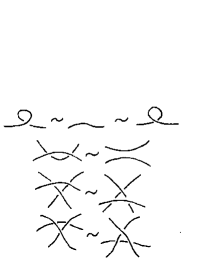
It turns out that two knots and are isotopic iff there exists a sequence of elemetary isotopies (called Reidemeister moves) between projection diagrams of and . The Reidemeister moves are given in diagrammatic representation in Fig. 1. The first move RI consists of modifying a diagram by putting a twist in the neighbourhood of a single strand. The second move RII consists of cancelling a pair of crossings. The third move consists of sliding a strand over a crossing (RIIIa) or under a crossing (RIIIb). There is also a “zeroth” move R0 which consists simply of an isotopy of the plane. We note that these moves are local; they are applied (one at a time) to one segment of a knot diagram while leaving the rest of the knot diagram unchanged. The equivalence relation generated by all Reidemeister moves except RI is called regular isotopy. Also, a loop that cannot be deformed into the unknot with the Reidemeister moves is said to be knotted.
3.2 Link Invariants
By Reidemeister’s theorem [29], the topological properties of knots and links in three-space ( or ) can be studied by working with diagrams of the knots taken up to the Reidemeister moves. That is, if diagrams for two knots or links are ambient isotopic in three-dimensional space iff the diagrams can be obtained one from another by a sequence of Reidemeister moves.
A knot or link is said to be oriented if a direction along the curve is chosen for each component of the knot or link. When we have a diagram of an oriented knot or link, then each crossing inherits and orientation sign. We define for right-handed orientation positive sign and for left-handed orientation negative sign . Let us first consider the self-linking number. For an oriented (one-component) knot diagram with crossings this is
| (40) |
We note that this function is not preserved under RI but is preserved by the other Reidemeister moves, and is therefore a regular isotopy invariant. Now let us consider an oriented diagram formed by two knots and . The linking number is
| (41) |
where the intersection does not include the self-crossings of or . As an example we will calculate the linking number for Hopf links with opposite orientations. For and so that we have
| (42) |
while for and so that we have
| (43) |
Before we go on to define the bracket polynomial we will introduce the notion of framing. Let be a knot that is defined by a closed curve . The framing of is a vector field that is normal to the curve , whose endpoints generate a boundary curve . So a framed knot can be visualized as a closed ribbon with boundaries defined by the curves and . The first Reidemeister move RI fails for framed knots. Instead, a curl in a diagram corresponds to a twist in the ribbon. See Fig. 2. We find that both and represent the same twist and so we set .
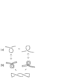
This modified deformation is henceforth labelled RI′.
Now we are ready to define the bracket polynomial. Let be a multi-component link containing crossings. A state of is obtained by choosing a smoothing of each crossing. Assigned to each crossing of is a choice , where the action of the vertex weights on the th crossing is given by
| (44) |
smoothing the crossing horizontally results in a multiplicative factor of while smoothing the crossing vertically results in a multiplicative factor of . The resulting state will be a finite set of disjoint circles of cardinality . The bracket polynomial is then a state sum given by
| (45) |
This is a polynomial in the commuting variables , and . The skein relations that define the bracket polynomial are
| (46) |
These equations follow directly from the definition of the state sum, where a normalization of unity has been employed for the unknot. Here does not intersect the added loop. Note that the bracket polynomial is an invariant of regular isotopy; if the axioms are applied to a twist then
| (47) |
In fact, the bracket polynomial is invariant under the framed Reidemeister moves for a specific choice of the commuting variables . As defined, the bracket polynomial is invariant under RI′, but fails for RII:
| (48) |
Invariance requires that and which uniquely determines the variables such that and . With this choice the bracket polynomial is now also invariant under the action of RIII. Now we can write the defining state sum (45) for framed links that is invariant under the Reidemeister moves as a polynomial in the single variable , with the skein relations
| (49) |
Let us now define the Jones polynomial. For a framed oriented link this is a polynomial in such that
| (50) |
The skein relations for this polynomial (with ) are
| (51) |
Now note the relation for the bracket polynomial under the action of RI for unframed links given by (47), with coefficients and . Under RI this extra factor acquired by the bracket polynomial is cancelled by the coefficient in the definition of the Jones polynomial above. The Jones polynomial is therefore an invariant of oriented links. The framing is irrelevant.
3.3 Link Invariants from Gauge Theory
The Jones polynomial was originally defined for knots and links in the three-sphere . We will proceed to show that the exponential of the Chern-Simons action as a measure provides an intrinsic definition of the Jones polynomial in an arbitrary three-dimensional manifold . The reader should note that the functional integral so defined is only understood heuristically. It is nevertheless, a powerful heuristic device, leading to a host of results. We might expect this because the Chern-Simons action is invariant under diffeomorphisms, so a change of basis to loop space (see below, where the loop transform is defined) should give a knot invariant for every gauge group . Let be an oriented closed curve in . We consider the Wilson loop
| (52) |
obtained by calculating the holonomy of the connection in the representation of the gauge group . Clearly the closed curve can be a knot; taking oriented and non-intersecting knots () whose union is a link , we define the partition function of the manifold such that
| (53) |
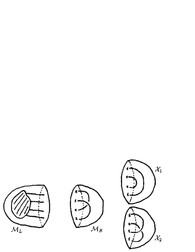
This is a path integral over all gauge orbits where we have assigned a representation of to each knot . The partition function above is the unnormalized expectation value of the given Wilson loop. Evaluating this path integral amounts to the determination of a vector in the physical Hilbert space , i.e. the space of gauge-invariant wavefunctions in the presence of Wilson loops. We will now consider the special case and . Assume that there is a link present in and we cut into two sections and . The boundaries of these sections will now be Riemann surfaces intersecting the link transversely in a set of marked points. In the case where there are four marked points and the Wilson lines are all in the same -dimensional representation of , then (we state without proof that) the physical Hilbert space will be two-dimensional. If the sections and are pasted back together, then the resulting link invariant may be the original, or may be a result of pasting with or with . This is illustrated in Fig. 3.
Now let and . Here is a vector associated to the boundary of , is a vector associated to the boundary of and is a vector associated to the boundary of . We note that any three vectors in a two-dimensional vector space are linearly dependent, and since are vectors contained in the same Hilbert space we have that
| (54) |
Here the constants . We may then postulate a natural pairing of vectors to the partition function , to the partition function and to the partition function . The relation (54) becomes
| (55) |
and this translates into a reccursion relation for the expectation values of the Wilson loops given by
| (56) |
Diagrammatically this is interpreted as
| (57) |
Now, the explicit evaluation of the constants would divert us too much from the main purpose of this paper, but it is neccessary to state the final result. The reader is referred to Witten’s paper [3] and references therein for details of the evaluation. For a connection of Chern-Simons theory with gauge group and all Wilson lines in the same -dimensional representation of , we have that
| (58) | |||||
| (59) | |||||
| (60) |
Multiply these by a factor and define a variable . Now (56) and (57) become
| (61) | |||||
| (62) |
This is the skein relation for the HOMFLY polynomial [30], which is the generalization of the Jones polynomial to . If we get the skein relation for the Jones polynomial.
Before moving on to gravitation, we will briefly discuss a simple case of the partition function (53) in order to illustrate a subtlety that arises when evaluating the path integral (53) for a specific case. Take and . The potentials commute so the cubic term in the Chern-Simons action vanishes, while the trace and path-ordering become irrelevant. Consider in two non-intersecting knots and . To the two different representations of we assign integers and . Evaluating the integral along the knots and in a region of that is essentially Euclidean space with and the coordinates along the knots, the partition function for the case becomes
| (63) |
This is the Gauss linking number, which was first written down by Gauss more than one hundred and fifty years ago! It is well defined provided that the two knots do not touch or intersect, because the integral diverges at the point . Witten regularized this divergence for the case by giving the knots a framing, and interpreted the resulting quantity as the self-linking number of one knot. Actually, this framing regularization is neccessary for all gauge groups. We have not mentioned it before because it was not relevant to the derivation of the skein relation, i.e. we did not need to evaluate any integrals. In a sense, we found a reccursion relation for Wilson loop expectations for unframed loops, thereby neglecting the self-linking. That is why we obtained the Jones Polynomial. Later we will see that the need for framing will arise naturally for a state of quantum gravity with non-zero cosmological constant. There we will obtain the bracket polynomial for , which depends on the framing.
4 The Gravitational Field: Classical Theory
4.1 Second Order Formulation
The use of tensors in general relativity is motivated by the principle of general covariance [31, 32], which states that the laws of physics must be independent of the coordinates being used. For example, the metric tensor relates distances in space and time via the invariant line interval , and may be seen as a generalization of the Pythagorean theorem to curved four-dimensional spacetime. The metric tensor is normally taken to be the dynamical field of the gravitational force. The equations relating the gravitational field to its source are the Einstein equations
| (64) |
Here the Ricci tensor encodes information about the curvature, and its contraction is the Ricci scalar. The material contents of the system, whatever it might be, are described by the stress-energy tensor . The quantity is the cosmological constant, which manifests itself as an acceleration whose magnitude increases with distance as in the weak-field limit. The dimensions carried by are , which implies that this term must be significant globally. The Einstein equations (64) can be derived from an action, either the Einstein-Hilbert action
| (65) |
by taking the Ricci scalar to be a functional of the metric, or equivalently the Hilbert-Palatini action
| (66) |
by taking the Ricci scalar to be a functional of the Christoffel coefficients of the second kind . The matter action is generally a function of the scalar field , spinor field and vector field in addition to the metric . The stress-energy tensor is obtained by varying the matter action with respect to the metric such that
| (67) |
It must be noted, however, that this tensor is not the same as the canonical stress-energy tensor that is obtained from the symmetries of the Lagrangian, i.e. Noether’s theorem. The equivalence only holds for a scalar field (up to a numerical factor). In general, the canonical stress-energy tensor will not even be symmetric, and in many cases such as electrodynamics, will not even be gauge invariant. Thus we define the stress-energy tensor as that which is obtained by variation of the matter action with respect to the gravitational field. When the action (65) and the action (66) are varied with respect to we get the Einstein equations. The virtue of using (66) over (65), however, is that variation of the former with respect to also gives the metric compatability condition .
4.2 First Order Formulation
The Einstein theory can also be formulated in terms of an orthonormal tetrad frame that satisfies
| (68) |
Locally then the manifold is flat Minkowski space and the curvature is encoded in the tetrad frame field. The covariant derivative acts on spacetime indices in the usual way:
| (69) |
In addition now the covariant derivative acts on Lorentz indices such that
| (70) |
This defines the spin connection . The spin connection determines the torsion two-form
| (71) |
the vanishing of the torsion implies the antisymmetry of the spin connection. This with the orthonormality of the tetrad leads to the metric compatibility condition and determines a unique connection on the manifold called the affine connection. With this connection are associated the connection coefficients . In terms of these the spin connection coefficients are . This is general and may be taken as the definition of the -coefficients. In a coordinate basis these are the Christoffel symbols of the second kind. Now it is clear that the metric compatibility condition implies that the spin connection is also compatible with the metric:
| (72) |
This can be inverted to give back (71). The spin connection also determines a curvature
| (73) |
the components of which determine the curvature two-form
| (74) |
Equations (71) and (74) are called the Cartan structure equations. If the tetrad is invertible then we can define the Ricci tensor and Ricci scalar . With this the Hilbert-Palatini action becomes
| (75) |
which up to boundary terms is invariant under local transformations and local translations. The matter action is generally a function of the scalar field , spinor field and vector field in addition to the gravitational field . Variation of the total action with respect to gives the Einstein equations
| (76) |
as the equations of motion, while variation with respect to gives the metric compatability condition. Here the stress-energy tensor defines the three-form .
4.3 Self-Dual Formulation
We finally come to the self-dual formulation of general relativity [33, 34, 35], which is the starting point for canonical quantization. To this end, we consider the integral
| (77) |
which is a topological term in the sense that it is invariant under local variations of the tetrad. An equivalent action for general relativity is therefore
| (78) | |||||
Now in terms of the spin connection the self-dual connection is given by
| (79) |
and this determines a self-dual curvature
| (80) | |||||
With this and a change of variable the self-dual action becomes
| (81) |
Variation of this action with respect to the tetrad field does give the Einstein equations as can be verified. Here the connection is complex so the metrics that satisfy the Einstein equations are complex-valued. To recover real general relativity certain reality conditions must be imposed on the phase space. In particular, we begin with complex general relativity on a real manifold, and, after defining the Hamiltonian using the self-dual connection, we restrict ourselves to the real section of the complex phase space. This is not very straightforward in practice, however, because it is not obvious that the pull-back of the symplectic structure to the real section is itself real. An alternative approach is to start with a real Ashtekar connection for Euclidean general relativity and later Wick rotate to Lorentzian general relativity. A more modern approach, however, is to use a form of Ashtekar variables with a real connection that describes Lorentzian general relativity, but at the price of having to solve a much more complicated Hamiltonian constraint. We will proceed to derive the gravitational Hamiltonian using this Barbero formulation [36] that describes the phase space of Lorentzian general relativity with a real connection. Later in Section 5.3 we will go back to the complex self-dual connection and derive the Kodama state for the simplified Hamiltonian constraint.
4.4 Classical Phase Space
The canonical structure is obtained using the usual ADM decomposition (see Appendix C). Without loss of generality we use the internal gauge symmetry of the gravitational field to fix the tetrad component . Now define on the time-slice the densitized triad of weight one and local connection , which are related to the phase space of the induced metric and extrinsic curvature by
| (82) |
Here is the connection of the triad. From this we can consider a more general connection given by [36]
| (83) |
where is an arbitrary parameter. If is real it is known as the Immirzi parameter. It does not play any role in classical dynamics because the extrinsic curvature term does not show up in the equations of motion unless the action contains fermions. (It was shown in [37] that appears in the equations of motion as the coupling constant of a four-point fermion interaction term.) In terms of the densitized triad and the connection in (83) the action becomes
| (84) |
Here we have seven first class constraints
| (85) | |||||
| (86) | |||||
| (87) | |||||
where and are the gauge covariant derivative and curvature of the connection . (The notation “” denotes weak equality on the constraint surface.) In the above action we identify the term as the analogue of the term “” in the Legendre transform . Thus the gravitational (Ashtekar) Hamiltonian is a linear combination of the constraints
| (88) |
The phase space is now described naturally by the connection (gauge potential) and its conjugate momentum (electric field). They satisfy the Poisson bracket relations
| (89) | |||||
| (90) |
Now we know that the first class constraints of a Hamiltonian system generate gauge transformations. General relativity is no exception. The three vector (diffeomorphism) constraints and scalar (Hamiltonian) constraint generate surface deformations that are equivalent to spacetime diffeomorphisms when the field equations hold. The algebra of these surface deformations is a Poisson algebra with structure functions rather than structure constants. We have now, in addition, the three “Gauss law” constraints that are typical of Yang-Mills theory. These generate the usual gauge transformations.
We make a final note on the canonical theory described here. The formulation in terms of the connection turns out to be a generalization of the Einstein theory. The equations in the metric formulation contain the Ricci scalar which requires the inverse metric to be defined. This means that the metric has to be non-degenerate. The phase space here is now determined by the set , so the metric is a derived quantity. Here all the equations of the Hamiltonian theory are polynomial, and the inverse triad does not appear in any of them. The theory is therefore well-defined even when the triad is degenerate, and therefore the theory admits solutions with a degenerate metric. If the triad is restricted to be non-degererate then the Einstein theory is recovered.
5 The Gravitational Field: Quantum Theory
5.1 Loop Representation
The phase space of general relativity is now defined and the canonical analysis is complete. What is left is to quantize the system. This is done by promoting the constraints (87) to operators , , ; these are required to annihilate physical states on the Hilbert space. In the connection representation the phase space variables become
| (91) |
Also the Poisson brackets on the phase space are promoted to commutators on the Hilbert space via . Of course this is quite difficult in practice due to ordering ambiguities. General relativity also suffers from the problem of time, structure functions of the surface deformation algebra etc. We will not go into the details here, but refer the reader to the book by Ashtekar [35], the review article by Rovelli [38] and the book by Rovelli [39].
The quantum constraints require that states be gauge invariant functionals of the connection. And so we are naturally led to consider Wilson loops defined by the self-dual connection. To this end we consider an spinor description for the canonical variables where and in terms of the spin half generators in the fundamental representation. (Here are the usual Pauli matrices.) We consider along a continuous piecewise smooth curve that is parametrized by (), the holonomy of the Ashtekar connection such that
| (92) |
This satisfies the differential equation
| (93) |
and the boundary condition ; this simply says that the vector in the vector bundle over the manifold is parallel transported along the curve . Hence the alternate name “parallel propagator” for the holonomy. Now we define the fundamental set of gauge-invariant loop operators (for ) [38, 39]. For a loop such that and the points we have:
| (94) | |||||
| (95) | |||||
| (96) | |||||
| (97) |
We will now proceed by introducing some notation for the loop variables that will be needed below. Let and be two loops, and be a segment of a curve. If and intersect at a point then the loop is obtained when starting at , going first through , then through and finally ending at . If a segment of a curve is glued to the loop then the result is denoted . Also the inverse of a loop or of a segment of a curve is just the loop or segment with opposite orientation. With this, the loop operators satisfy the properties:
| (98) | |||||
| (99) | |||||
| (100) | |||||
| (101) |
Here is a loop centered at the point on the spatial manifold with area . Finally we write down the (closed) Poisson algebra of the lowest-order operators and :
| (102) | |||||
| (103) | |||||
| (104) | |||||
| (105) |
Here we have introduced the notation to mean that the breaking and rejoining of the loops occurs at the intersection of the two loops where the parameter is , and we have defined the structure functions
| (106) |
Note that if the loops do not intersect then the Poisson brackets vanish. These can be obtained with rigor by using the operator definition for the field. It is to be understood that these relations define the Poisson brackets and are not the usual Poisson brackets that are defined by derivations. The relations above are called the -algebra, and realizes Isham’s proposal [13] of employing a non-canonical Poisson algebra for the quantization of general relativity.
Let us now prove that loop states solve the constraints of the phase space of general relativity. We will do this for any arbitrary loop state. We have already encountered a gauge invariant loop, namely the Wilson loop, which is just the trace of the holonomy of the Ashtekar connection. The gauge invariance implies that this quantity automatically solves the Gauss constraint . In addition, it is an exact solution to the scalar constraint . So let us consider a general functional of the form
| (107) |
where is a loop contained in the set of differentiable non-intersecting loops . Then for a functional in the connection representation and a functional in the loop representation, we define the loop transform [10, 11]
| (108) |
Here is a measure on the space of connections that is assumed to be invariant under diffeomorphisms. The transform is therefore a mapping . Operators in the two representations are related to each other through the transform in the following way. Let be an operator acting on the space of connections and let be an operator acting on the space of loops. Then and are related through the transformation
| (109) |
provided that . Now, the loop transform is the key to understanding how the loop functionals solve all constraints in the loop representation. It is known that the Wilson loop satisfies and . Therefore the kernel also satisfies and , and it follows that the functional in the loop representation satisfies the constraints for any choice of functional in the connection representation. All that remains now is to impose the vector constraints . However, diffeomorphisms map loops to other loops in the same knot class, so we conclude that will satisfy all constraints provided that the functional depends on the knot classes of loops.
5.2 The Spin Network Basis
The most beautiful result of loop quantum gravity is the discretization of the spatial manifold. The non-perturbative quantization of the gravitational field leads to quantum geometry operators with discrete spectra. Details on this can be found in [39, 40] and references therein. A self-contained exposition on the calculation of geometry eigenvalues based on Temperley-Lieb recoupling theory [41] can be found in [42]. The area operator, for example, has been used to calculate the Bekenstein-Hawking entropy for an extremal black hole [43, 44, 45, 46]. This result was used to fix the Immirzi parameter.
Functionals in the loop representation that diagonalize the area and volume operators are represented by combinatorial structures called spin networks. A spin network state [42] is a combination of loops called a graph , containing a certain number of edges and vertices. To each edge we assign a half-integer (spin) which labels an irreducible representation of , and to each vertex we assign an invariant tensor called an intertwiner in the tensor product of the representations at which the spins join. A spin network is then the set
| (110) |
Note that is an abstract spin network. The embedding of into the spatial manifold is an embedded spin network. The distinction should be clear from context. Essentially we find the holonomy of the connection in the representation and use the tensor at each vertex to obtain an invariant functional. The result is then a state in the connection representation. The spin network states are linearly independent and provide an orthogonal basis for the kinematical Hilbert space [38, 39]. In fact, we can write any state in the connection representation as a superposition . The coefficient here is the inner product
| (111) |
where the diffeomorphism invariant measure is over the gauge equivalent classes of generalized connections . The configuration space is a canonical enlargement of [47, 48, 49, 50]. The enlargement is neccessary if the loop operators are to remain well defined in the quantum theory where the number of degrees of freedom is infinite. This measure has only been defined rigorously for . In the next section we will discuss the case . There, we will see how the loop transform is related to Witten’s partition function when we discuss the Kodama wavefunction, and obtain a known topological invariant as an exact quantum state in the loop representation. As we will see, the presence of can be incorporated into the measure of Chern-Simons theory.
5.3 An Exact State
Recall the scalar constraint in (87). If we set as for the self-dual connection, then the last term vanishes and we get
| (112) |
This is the Hamiltonian constraint in the original self-dual formulation. It is clear that a solution to this (and also to and ) will have to satisfy
| (113) |
If is chosen for the connection with arbitrary function , then the curvature becomes . Now the connection defined in (82) is purely imaginary so the connection of the triad vanishes which means that is a flat manifold. The canonical momentum becomes so that the spatial metric is . To find the evolution equation for we write down the Hamilton equations of motion for the canonical variables:
| (114) |
For simplicity we take the shift vector in (88) to be zero. In other words, the spacetime metric has no - cross terms. The evolution for is then given by , and taking the lapse function leads to or . So the line element is
| (115) |
which is immediately recognized as de Sitter spacetime. This is also a Friedmann-Robertson-Walker spacetime with flat spatial manifold and scale factor . It is the only self-dual solution to the Einstein equations for Lorentzian manifolds. Now, to see how this solution is related to topological field theory in , we take to be a Hamilton-Jacobi functional on the space of connections in . This implies that the canonical momentum is
| (116) |
but from the curvature (113) we have then
| (117) |
In terms of the curvature is
| (118) |
Integration then gives the Hamilton-Jacobi functional
| (119) |
From this we are led to the semiclassical state
| (120) |
which describes de Sitter spacetime. This state is, however, an exact state in quantum gravity. It is annihilated by all the constraints:
| (121) |
This means that is a physical state of non-perturbative quantum gravity with a non-zero cosmological constant [51]. This is the Kodama state, whose classical limit is de Sitter spacetime. States of the form
| (122) |
can then be used to obtain linearized gravity on de Sitter spacetime, i.e. gravitons propagating over a classical background. The normalization factor satisfies , and depends on the topology of the manifold. In fact, Soo [52] pointed out that a more general solution would sum over all inequivalent topologies of so that
| (123) |
The boundary of is required to vanish so that is still annihilated by all the constraints. This sum, however, is very large and in fact unknown, because a complete classification of three-manifolds is lacking at this time.
Finally we come to a very striking property of the Kodama state, which serves as a point of convergence for all the material that has been discussed up to this point. So let us take the loop transform of the Kodama state. Allowing for either Euclidean or Lorentzian manifold by introducing the integer , we have
| (124) |
We want to be able to evaluate the loop transform for states with so as to include the Kodama state. The above integral, however, is undefined unless the loops are framed. With this framing regularization the group of spin networks becomes “quantum deformed” to with deformation parameter
| (125) |
Clearly then for , . For Euclidean manifold this is exactly Witten’s partition function with gauge group and the Wilson loops all in the same two-dimensional fundamental representation of . In loop space the Euclideanized Kodama state is then the bracket polynomial in the variable . Unfortunately, this picture is a bit more difficult for the Lorentzian case because now the integral (124) has to be taken over a contour since the connection is complex. It is possible to analytically continue the deformation parameter to complex values of the Chern-Simons level. With the loops now framed, the spin networks become essentially blown up to a two-dimensional surface [53, 54, 55]. Edges become tubes with ruling. The ruling means that the original loop before deformation can be identified. Vertices become spheres with punctures, each puncture being the location where a tube intersects the sphere. The punctures are now labelled by intertwiners of the quantum group . The intertwiners depend on the level of the Chern-Simons theory, and are none other than the space of conformal blocks. The reader will find this easy to visualize if he/she thinks of the spin networks as just trivalent graphs and replaces the edges by tubes and the vertices by junctures of tubes that form non-singular surfaces. We refer the reader to the literature cited in this subsection for the handling of framing with respect to the networks and the surfaces.
Now the picture is complete. Functionals of non-perturbative quantum gravity with a positive cosmological constant in the loop representation are finite-genus ruled Riemann surfaces with marked points. It is remarkable that the structures which naturally describe perturbative string theory [56, 19] have emerged as functionals of a non-perturbative quantization of the gravitational field. One thing still lacking in perturbative string theory is a background-independent formulation called M(ystery) theory. An ambitious program launched by Smolin [57, 58, 59, 60] is to describe M theory as a deformation of abstract spin networks.
6 Outlook
In this review we discussed in detail non-Abelian Chern-Simons theory for arbitrary gauge group on a three-dimensional manifold with boundary. We examined the relation of this field theory to the WZW conformal field theory in two dimensions and saw that, after canonical quantization, the wavefunctions of the Chern-Simons theory are the conformal blocks of the WZW current algebra at level . By using the Chern-Simons action as the measure of a path integral which defines the expectation value of the Wilson loop, we described Witten’s intrinsic three-dimensional definition for the Jones polynomial. We then described a reformulation of general relativity on an Yang-Mills phase space, and defined the fundamental loop representation of the non-canonical -algebra for which led to a purely combinatorial structure called the spin network. For we solved the constraints to obtain an exact state of quantum gravity whose classical limit is de Sitter spacetime. The presence of led to the framing of loops and therefore to a quantum deformation of the spin networks, resulting in a discrete spacetime of punctured Riemann surfaces with finite genus.
In loop quantum gravity, we have understood that via the loop transform one can represent states of quantum gravity via Wilson loops (and integrals of Wilson loops over the underlying gauge field ), and hence by the geometry of knots and links embedded in the three-space. The loop transform associates a functional integral to a given loop in three-space, and it is seen that in the case of the Chern-Simons state that this transform is, up to framing, a topological invariant of the loop (as discussed in more detail below). One knows that these same topological invariants arise by taking bracket evaluations of the knots at appropriate values of the bracket variable . As a result, it is a well-grounded move to shift from the functional integral approach to an approach that evaluates knotted and embedded spin networks in three-dimensional space. Each such evaluation can be regarded as a specific evaluation of a quantum gravity loop transform, and one can look for geometric and physical intepretations of these evaluations. One can think of each loop state as having all its geometry concentrated along the loop in the fashion of a three-dimensional embedded delta function. The metric that arises here assigns an area measurement to any test two-dimensional surface that encounters the spin network loop. Each intersection point gives the value , where labels the spin network edge, and we have retained the speed of light and Planck’s constant . One adds up all the contributions to the area coming from the different spin network lines in a given or chosen family of embedded spin networks in three-dimensional space. The remarkable point about this method is that in the context of loop quantum gravity, the area measurements are quantized in this fashion. The fundamental quantum of area is given by a surface with a single puncture, with the edge carrying a spin . In this case . Surfaces make quantum jumps between states in the spectrum of the area operator. This, in turn reflects on many other issues such as the discrete nature of space and time at the Planck scale and the information content of black holes. For more information on these and related matters we refer the reader to [43, 44, 45, 46, 61, 62, 63, 64, 65].
Having discussed the achievements of the approach to quantum gravity presented in this review, we will now turn to a brief discussion of several key problems that are still open. These include:
-
•
The physical Hilbert space: Time evolution is governed by the Wheeler-de Witt equation , where is the operator corresponding to the complicated Hamiltonian constraint in (87). The theory should express four-diffeomorphism invariance but the canonical decomposition requires a choice of external time parameter, thus breaking general covariance. The states described here form the “kinematical” Hilbert space; that is, these states only solve the quantum constraints and . What is needed is a set of functionals that will solve the Wheeler-de Witt equation and define the physical Hilbert space, and on it a physical inner product. A possible candidate for the Wheeler-de Witt operator has been defined by Thiemann in [66], but it is not obvious that this operator in the classical limit describes general relativity at all.
-
•
Reconstruction problem: Any candidate theory of quantum gravity should in some limit reproduce a classical background metric that satisfies the Einstein equations. Furthermore, we expect that a good theory of quantum gravity coupled to matter should in some low-energy limit reproduce quantum field theory in curved spacetime. This is, however, a very non-trivial problem to address. Matter has been coupled to gravity via the self-dual variables and has been quantized [67, 68, 69, 71, 70]. The problem has only been solved on the kinematical Hilbert space. As mentioned above, an inner product for physical states is currently lacking in loop quantum gravity. Therefore the dynamics of matter coupled to gravity, as for example transition amplitudes to describe scattering processes within this framework is currently still out of reach.
-
•
Normalization of the Kodama wavefunction: An analogous wavefunction to the Kodama state exists for Yang-Mills theory given by
(126) where is the coupling constant and is given in (119). This state is a solution to with . Witten [72] pointed out that the physical norm of this theory, which is given by
(127) is infinite because the configuration space is unbounded from below. He conjectured that this should be true also for the Kodama state. This issue is addressed in [73], where it is argued that this argument does not extend to gravity because the Kodama state, as any other states that are physical states, are expected to be nonnormalizable in the kinematical inner product. The Yang-Mills theory above is not diffeomorphism-invariant and hence the state (126) is nonnormalizable in the physical inner product. In [73], in order to address the issue of normalizability in the physical inner product, the authors studied the linearized Kodama state over a de Sitter background. They found that although this linearized state is delta-function normalizable in the Euclidean theory, it is not normalizable in the Lorentzian theory. This raises an important issue as to whether the full Kodama state discussed in this paper is a physically reasonable state to describe the ground state of quantum gravity with a positive cosmological constant.
Most of these issues may be solved in the future using the state sum and spin foam models for quantum gravity that are currently under intensive investigation. These are based on a covariant path integral approach and hence do not break general covariance. There is not room in this short review to do more than mention these aspects. We refer the reader to [74, 75, 76, 77, 78, 79, 80, 81, 82, 83] for more information on state sum models and [84, 85, 86, 87, 88] for more information on spin foam models. Several important problems have now been addressed in this direction:
- •
-
•
Work is in progress on spin foam models of matter coupled to quantum gravity [91, 92, 93]; the question of particle scattering within the framework of background-independent quantum gravity has been addressed in [94]; an attempt has been made at obtaining the graviton propagator via spin foams in [95].
-
•
Recently the idea has been put forward, that perturbative quantum gravity can be treated as an expansion around topological theory [96]. This is related to the fact that gravity can be written as theory with the constraint that the field comes from the metric. An implementation of this idea has been applied to standard Yang-Mills theory in flat spacetime [97] and was shown to be a viable technique for perturbation theory of generally covariant theories.
We conclude with a few remarks on the background dependence of matter quantum field theories. There it is always assumed from the outset that the background spacetime is continuous to arbitrarily small scales. In the non-perturbative quantization of pure gravity we generically end up with a discrete space with length, area and volume eigenvalues. So the initial assumption of quantum field theory is false in this context, and may in fact be the origin of the ultraviolet divergences that plague the quantum field theories. Indeed in his QSD V article, Thiemann [98] shows that the divergences can be fully accounted for if we neglect the discreteness of space, and has argued that the Planck scale may provide a natural cutoff regularization of the Hamiltonian constraint of matter quantum field theories. We can go further. By looking at the modifications to matter interactions after taking the discreteness of space into account, we may find a better understanding of nature, built on a well-defined set of principles.
Acknowledgments
This review is an expanded version of a report that was written for a graduate course on knots and quantum gravity, taken by T.L. during the summer of 2004 at the University of Waterloo. T.L. is supported by the Natural Sciences and Engineering Research Council of Canada under grant 101203.
It gives L.H.K. pleasure to thank the National Science Foundation for support of this research under NSF Grant DMS-0245588. Much of his effort was sponsored by the Defense Advanced Research Projects Agency (DARPA) and Air Force Research Laboratory, Air Force Materiel Command, USAF, under agreement F30602-01-2-05022. The U.S. Government is authorized to reproduce and distribute reprints for Government purposes notwithstanding any copyright annotations thereon. The views and conclusions contained herein are those of the authors and should not be interpreted as necessarily representing the official policies or endorsements, either expressed or implied, of the Defense Advanced Research Projects Agency, the Air Force Research Laboratory, or the U.S. Government. (Copyright 2005.)
The authors would both like to thank the University of Waterloo and the Perimeter Institute for their hospitality during much of the work on this paper.
The authors would also like to thank Kirill Krasnov for comments, and the referees for pointing out several errors in an earlier draft of the manuscript, and for their suggestions which improved the presentation of the review.
Appendix A Conventions
Here we collect the conventions used in the paper. Unless otherwise stated, we work on a four-dimensional Lorentzian manifold which admits constant time hypersurfaces . We use the following index conventions: lower-case greek letters are spacetime indices; lower-case roman letters are spatial indices; upper-case roman letters are internal tangent space indices; upper-case roman letters with hats are gauge-fixed internal tangent space indices. Spacetime indices are raised and lowered with the spacetime metric , spatial indices are raised and lowered with the induced spatial metric on a constant time slice, and internal indices are raised and lowered with the Minkowski metric . Here spacetime and spatial indices are consistently written before the tangent space indices for all quantities on . The Einstein summation convention is used for repeated upper and lower indices. Units are employed for which the speed of light and Planck’s constant are unity, and Newton’s constant is retained.
Appendix B Hamiltonian Formulation of Classical Mechanics
For convenience we summarize here the Hamiltonian formulation of a classical unconstrained system with a finite number of degrees of freedom [99, 100]. We consider a system that is governed by the action , where is an integration parameter with an overdot denoting , and is known as the system’s Lagrangian. This is a functional, and is defined as the kinetic energy minus the potential energy. In most cases the kinetic energy is a function of the system’s velocities and the potential energy is a function of the system’s coordinates . The set of all coordinates are said to define an dimensional manifold called the configuration space . However, the defining action exludes the more interesting gauge theories because the Lagrangian only describes systems with a finite number of degrees of freedom. For the former we would need to consider . Furthermore, the parameter in most nonrelativistic systems is the time which measures evolution, but this breaks down when we consider relativistic motion since time is no longer a parameter.
Now, the functional is differentiable, and the equations of motion of the system are obtained by demanding that the action be stationary with respect to variations of and . We find that
| (128) |
Here we integrated by parts using . The boundary term vanishes because we are taking the variation with respect to fixed endpoints. If we impose for arbitrary , then it follows that
| (129) |
This is a set of second order differential equations in , , and . These are called the Euler-Lagrange equations of motion, and by Hamilton’s principle of least action (which states that the motion of a mechanical system coincides with the extremals of the functional ) determine the (time) evolution of the system. Furthermore, the canonical (generalized) momenta of the system are given by
| (130) |
these are of central importance in the Hamiltonian formulation to be introduced below. They are generalized momenta in the sense that they represent a generalization of the Newtonian notion of momenta given by . Equations (129) can be shown to reproduce Newton’s second law in the form .
An equivalent approach to Lagrangian mechanics outlined above is to use a Legendre transform to obtain a set of first order differential equations to replace (129). To this end, we let and . Now, we define the Hamiltonian function through the Legendre transform
| (131) |
The differential of this function is
| (132) | |||||
In general, however, we should expect the Hamiltonian to have differential of the form
| (133) |
Comparing this to (132) we obtain the Hamilton equations of motion
| (134) |
for which the Lagrangian must satisfy . If the transformations connecting the rectangular and canonical coordinates are independent of time so that the kinetic energy is a homogeneous quadratic function of the , and the potential energy is independent of velocity, then it follows that the Hamiltonian is equal to the total energy of the system and is a conserved quantity provided it does not explicitly depend on time. In fact, the Hamiltonian is a conserved quantity provided that the system is closed, i.e. a system which does not interact with its surroundings.
Let’s now consider a function denoted by , for which we calculate the total time derivative to be
| (135) | |||||
Here we made use of the Hamilton equations (134). This can be written more abstractly if we define the Poisson bracket111The Poisson bracket satisfies the following identities: 1. 2. 3. 4.
| (136) |
so that
| (137) |
In most cases will contain time dependence implicitly so that , and thus we have
| (138) |
This beautiful expression contains in it all of classical mechanics. If we evaluate the Poisson bracket for and we obtain the equations (134). In this form, we see that the Hamiltonian is the generator of time translations. The set of all coordinates are said to define a dimensional manifold called the phase space . A point on is called a state, and a function on that satisfies Hamilton’s equation is called an observable. The set of second order equations on have been replaced by a set of first order equations on .
A more absract formulation can be obtained if we define the phase space as a dual tangent bundle, or cotangent bundle, with coordinates on which the Hamiltonian is defined. This can be seen in the following way. Recall that the Lagrangian is defined over an -dimensional manifold called the configuration space . The are the components of a vector at the point . Thus the Lagrangian is a function on the tangent bundle. Now the Hamiltonian is obtained from the Legendre transform (131). The first term can be visualized as a pairing of an element of the tangent space with its dual. In replacing with as the new set of independent variables, the Legendre transform replaces the tangent bundle with the cotangent bundle and thus defines the Hamiltonian as a function . This explains why in the Einstein summation for some canonical set of variables we write the position with contravariant index and the momentum with covariant index.
The connection between conserved quantities and the symmetries of a Lagrangian is contained in Noether’s theorem. The essence of this theorem is that, if the Lagrangian is unaffected by a transformation that alters one of its coordinates, then the Lagrangian is invariant, or symmetric, under the given transformation, and the corresponding current is then conserved. In particular, there are seven constants associated with the motion of a closed system: homogeneity of time implies that the Lagrangian is invariant under time translations, which leads to the conservation of energy; homogeneity of space implies that the Lagrangian is invariant under spatial translations, which leads to the conservation of linear momentum; isotropy of space implies that the Lagrangian is invariant under spatial rotations, which leads to the conservation of angular momentum. In the Hamiltonian formulation, a conserved quantity is simply one for which the Poisson bracket vanishes, i.e. . This provides a simple proof of the conservation of energy since must be satisfied by the antisymmetry property of the Poisson bracket. Finally, we define a cyclic coordinate to be one that does not appear explicitly in the Lagrangian. Then (129) reduces to , in which case the Hamiltonian does not explicitly depend on either. Thus the canonical momentum conjugate to a cyclic coordinate is conserved, i.e. .
Appendix C ADM Decomposition
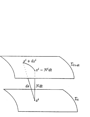
In order to cast the Einstein-Hilbert action with into Hamiltonian form, we need a time with which we can define the conjugate momenta. To this end, we split the spacetime into a space and a time. We assume that has the topology where is an open or closed three-dimensional surface; this is a segment of a universe between initial surface and final surface both assumed to be spacelike. We also assume the existence of constant time hypersurfaces endowed with coordinate systems and induced metrics . After an infinitesimal time translation from to , the change in proper time will be , and this leads in general to a spatial shift . Here is the lapse function and is the shift vector. The spacetime interval between two points and on is then
| (139) |
This is shown in Fig. 4. In components this gives the metric tensor and its inverse
| (142) | |||||
| (145) |
Here is the inverse of . From the form of the inverse metric above we note that are not the spatial components of .
Using the induced metric we can determine the curvature tensor that is intrinsic to the hypersurfaces . This is determined by parallel transporting tangent vectors on . However, we can also define an extrinsic curvature to describe how the hypersurfaces curve with respect to the embedding spacetime. This is described by the behaviour of vectors normal to . For a unit normal to in the lapse and shift decomposition above, this is given by
| (146) |
and with this we find that the Einstein-Hilbert action becomes
| (147) | |||||
Details can be found in [101, 102]. The canonical momenta can now be read off from the action:
| (148) | |||||
| (149) | |||||
| (150) |
There are four primary constraints and . The first momentum can be inverted to give the extrinsic curvature
| (151) |
and hence the action (147) becomes
| (152) | |||||
| (153) | |||||
| (154) |
Here, the Hamiltonian constraint and momentum constraints are secondary constraints, and the lapse and shift are Lagrange multipliers. The action (154) is in the form of a Lagandre transform for which the term plays the role of the term “”. Thus we identify the quantity as the gravitational Hamiltonian (called the ADM Hamiltonian for Arnowitt-Deser-Misner). Because the Hamiltonian is a linear combination of constraints it vanishes on-shell (i.e. when the equations of motion are satisfied). From we find the equal-time Poisson brackets
| (155) | |||||
| (156) | |||||
| (157) |
and for any function .
References
- [1] Gauss J C F Werke (Knigliche Geselschaft der Wissenschaften, Gtingen 1833) Volume V page 605 note of January 22
- [2] Ashtekar A and Corichi A 1997 Gauss linking number and the electromagnetic uncertainty principle Phys. Rev. D 56 2073
- [3] Witten E 1989 Quantum field theory and the Jones polynomial Commun. Math. Phys. 121 351
- [4] Maxwell J C 1873 Treatise on Electricity and Magnetism (Clarendon Press, Oxford)
- [5] Kelvin W T and Tait P G 1867 Treatise on Natural Philosophy (Cambridge University Press, Cambridge)
- [6] Tait P G 1898 On Knots I, II and III; Scientific papers, Vol. I (Cambridge University Press, Cambridge)
- [7] Jones V F R 1985 A polynomial invariant for knots via Von Neumann algebras Bull. Am. Math. Soc. 12 103
- [8] Einstein A 1905 On the electrodynamics of moving bodies Annalen Phys. 17 891
- [9] Kauffman L H 1987 State models and the Jones polynomial Topology 26 395
- [10] Rovelli C and Smolin L 1988 Knot theory and quantum gravity Phys. Rev. Lett. 61 1155
- [11] Rovelli C and Smolin L 1990 Loop space representation of quantum general relativity Nucl. Phys. B 331 80
- [12] Jacobson T and Smolin L 1988 Nonperturbative quantum geometries Nucl. Phys. B 299 285
- [13] Isham C and Kakas A C 1984 A group theoretical approach to the canonical quantisation of gravity: I. Construction of the canonical group Class. Quantum Grav. 1 621
- [14] Penrose R 1971 Angular momentum: An approach to combinatorial spacetime Quantum Theory and Beyond ed T Bastin (Cambridge University Press, Cambridge)
- [15] Kodama H 1988 Specialization of Ashtekar’s formalism to Bianchi cosmology Prog. Theor. Phys. 80 1024
- [16] Kodama H 1990 Holomorphic wavefunction of the Universe Phys. Rev. D 42 2548
- [17] Husain V 1989 Intersecting loop solutions of the Hamiltonian constraint of quantum general relativity Nucl. Phys. B 313 711
- [18] Brgmann B, Gambini R and Pullin J 1992 Jones polynomials for intersecting knots as physical states of quantum gravity Nucl. Phys. B 385 587
- [19] Hatfield B 1992 Quantum Field Theory of Point Particles and Strings (Westview Press, Boulder)
- [20] Baez J and Muniain J P 1994 Gauge Fields, Knots and Gravity (World Scientific, Singapore)
- [21] Loll R 1994 Gauge theory and gravity in the loop representation Canonical Gravity: From Classical to Quantum eds J Ehlers and H Friedrich (Springer-Verlag, Berlin)
- [22] Gambini R and Pullin J 1996 Loops, Knots, Gauge Theories and Quantum Gravity (Cambridge University Press, Cambridge)
- [23] Jackiw R 1984 Topological investigations of quantized gauge theories Relativity, Groups and Topology II ed B S De Witt (North-Holland, Amsterdam)
- [24] Carlip S 1991 Inducing Liouville theory from topologically massive gravity Nucl. Phys. B 362 111
- [25] Knizhnik V G and Zamolodchikov A B 1984 Current algebra and Wess-Zumino model in two dimensions Nucl. Phys. B 247 83
- [26] Witten E 1984 Non-Abelian bosonization in two dimensions Commun. Math. Phys. 92 455
- [27] Gaberdiel M R 2000 An introduction to conformal field theory Rep. Prog. Phys. 63 607
- [28] Belavin A A, Polyakov A M and Zamolodchikov A B 1984 Infinite conformal symmetry in two-dimensional quantum field theory Nucl. Phys. B 241 333
- [29] Reidemeister K 1948 Knotentheorie (Chelsea, New York)
- [30] Freyd P, Yetter D, Hoste J, Lickorish W B R, Millet K and Ocneanu A 1985 A new polynomial invariant of knots and links Bull. Am. Math. Soc. 12 239
- [31] Wald R M 1984 General Relativity (University of Chicago Press, Chicago)
- [32] Carroll S M 2004 Spacetime and Geometry: An Introduction to General Relativity (Addison-Wesley, San Francisco)
- [33] Ashtekar A 1986 New variables for classical and quantum gravity Phys. Rev. Lett. 57 2244
- [34] Ashtekar A 1987 New Hamiltonian formulation of general relativity Phys. Rev. D 36 1587
- [35] Ashtekar A 1991 Lectures on non-perturbative canonical gravity (World Scientific, Singapore) notes prepared in collaboration with R S Tate
- [36] Barbero F 1995 Real Ashtekar variables for Lorentzian signature space-times Phys. Rev. D 51 5507
- [37] Perez A and Rovelli C 2005 Physical effects of the Immirzi parameter Preprint gr-qc/0505081
- [38] Rovelli C 1991 Ashtekar formulation of general relativity and loop-space non-perturbative quantum gravity: A report Class. Quantum Grav. 8 1613
- [39] Rovelli C 2004 Quantum Gravity (Cambridge University Press, Cambridge)
- [40] Ashtekar A and Lewandowski J 2004 Background independent quantum gravity: a status report Class. Quantum Grav. 21 R53
- [41] Kauffman L H and Lins S L 1994 Temperley-Lieb Recoupling Theory and Invariants of Three-Manifolds (Princeton University Press, Princeton)
- [42] De Pietri R and Rovelli C 1996 Geometry eigenvalues and the scalar product from recoupling theory in loop quantum gravity Phys. Rev. D 54 2664
- [43] Rovelli C 1996 Black hole entropy from loop quantum gravity Phys. Rev. Lett. 77 3288
- [44] Krasnov K V 1997 Geometrical entropy from loop quantum gravity Phys. Rev. D 55 3505
- [45] Krasnov K V 1998 On quantum statistical mechanics of a Schwartzschild black hole Gen. Rel. Grav. 30 53
- [46] Ashtekar A, Baez J, Corichi A and Krasnov K 1998 Quantum geometry and black hole entropy phys. Rev. Lett. 80 904
- [47] Ashtekar A and Isham C J 1992 Representations of the holonomy algebras of gravity and non-Abelian gauge theories Class. Quantum Grav. 9 1433
- [48] Baez J 1994 Generalized measures in gauge theories Lett. Math. Phys. 31 213
- [49] Ashtekar A and Lewandowski J 1995 Projective techniques and functional integration for gauge theories J. Math. Phys. 36 2170
- [50] Ashtekar A and Lewandowski J 1995 Differential geometry on the space of connections via graphs and projective limits J. Geom. Phys. 17 191
- [51] Smolin L 2002 Quantum gravity with a positive cosmological constant Preprint hep-th/0209079
- [52] Soo C 2002 Wavefunction of the Universe and Chern-Simons perturbation theory Class. Quantum Grav. 19 1051
- [53] Smolin L 1995 Linking topological quantum field theory and nonperturbative quantum gravity J. Math. Phys. 36 6417
- [54] Borissov R, Major S and Smolin L 1996 The geometry of quantum spin networks Class. Quantum Grav. 13 3183
- [55] Major S and Smolin L 1996 Quantum deformation of quantum gravity Nucl. Phys. B 473 267
- [56] Green M B, Schwarz J H and Witten E 1987 Superstring Theory Vols I and II (Cambridge University Press, Cambridge)
- [57] Markopoulou F and Smolin L 1998 Quantum geometry with intrinsic local causality Phys. Rev. D 58 084032
- [58] Markopoulou F and Smolin L 1998 Nonperturbative dynamics for abstract string networks Phys. Rev. D 58 084033
- [59] Smolin L 2000 Strings as perturbations of evolving spin networks Nucl. Phys. (Proc. Suppl.) 88 103
- [60] Smolin L 2000 Candidate for a background independent formulation of M theory Phys. Rev. D 62 086001
- [61] Ashtekar A, Rovelli C and Smolin L 1992 Weaving a classical metric with quantum threads Phys. Rev. Lett. 69 237
- [62] Rovelli C and Smolin L 1995 Discreteness of area and volume in quantum gravity Nucl. Phys. B 442 593
- [63] Ashtekar A and Lewandowski J 1997 Quantum theory of geometry I: Area operators Class. Quantum Grav. 14 A55
- [64] Krasnov K 1998 The area spectrum in quantum gravity Class. Quantum Grav. 15 L47
- [65] Major S 1999 A spin network primer Am. J. Phys. 67 972
- [66] Thiemann T 1996 Anomaly-free formulation of non-perturbative, four-dimensional Lorentzian quantum gravity Phys. Lett. B 380 257
- [67] Rovelli C and Morales-Tecotl H (1995) Fermions in quantum gravity Phys. Rev. Lett. 72 3602
- [68] Rovelli C and Morales-Tecotl H (1995) Loop space representation of quantum fermions and gravity Nucl. Phys. B 451 325
- [69] Baez J and Krasnov K 1998 Quantization of diffeomorphism-invariant theories with fermions J. Math. Phys. 39 1251
- [70] Montesinos M and Rovelli C 1998 The fermionic contribution to the spectrum of the area operator in non-perturbative quantum gravity Class. Quantum Grav. 15 3795
- [71] Thiemann T 1998 Kinematical Hilbert spaces for fermionic and Higgs quantum field theories Class. Quantum Grav. 15 1487
- [72] Witten E 2003 A note on the Chern-Simons and Kodama wavefunctions Preprint hep-th/0306083
- [73] Freidel L and Smolin L 2004 The linearization of the Kodama state Class. Quantum Grav. 21 3831
- [74] Barrett J W and Crane L 1997 Relativistic spin networks and quantum gravity J. Math. Phys. 39 3296
- [75] Barrett J W and Crane L 2000 A Lorentzian signature model for quantum general relativity Class. Quantum Grav. 17 3101
- [76] Crane L 2000 Hypergravity and categorical Feynmanology Preprint gr-qc/0004043
- [77] Crane L, Perez A and Rovelli C 2001 A finiteness proof for the Lorentzian state sum spin foam model for quantum general relativity Preprint gr-qc/0104057
- [78] Crane L 2001 A new approach to the geometrization of matter Preprint gr-qc/0110060
- [79] Crane L and Yetter D 2003 A more sensitive Lorentzian state sum Preprint gr-qc/0301017
- [80] Crane L and Yetter D 2003 Measurable categories and 2-groups Preprint gr-qc/0305176
- [81] Alexander S, Crane L and Sheppeard M D 2003 The geometrization of matter proposal in the Barrett-Crane model and resolution of cosmological problems Preprint gr-qc/0306079
- [82] Crane L 2003 2-categorical Poincare representations and state sum applications Preprint math.QA/0306440
- [83] Christensen J D and Crane L 2004 Causal sites as quantum geometry Preprint gr-qc/0410104
- [84] Reisenberger M P 1997 A lattice world sheet sum for 4D Euclidean general relativity Preprint gr-qc/9711052
- [85] Baez J C 1998 Spin foam models Class. Quantum Grav. 15 1827
- [86] Freidel L and Krasnov K 1999 Spin foam models and the classical action principle Adv. Theor. Math. Phys. 2 1183
- [87] Oriti D 2001 Space-time geometry from algebra: Spin foam models for nonperturbative quantum gravity Rept. Prog. Phys. 64 1489
- [88] Perez A 2003 Spin foam models for quantum gravity Class. Quantum Grav. 20 R43
- [89] Markopoulou F 2000 An algebraic approach to course-graining Preprint hep-th/0006199
- [90] Markopoulou F 2003 Coarse graining in spin foam models Class. Quantum Grav. 20 777
- [91] Mikovic A 2002 Spin foam models of matter coupled to gravity Class. Quantum Grav. 19 2335
- [92] Mikovic A 2002 Spin foam models of Yany-Mills theory coupled to gravity Class. Quantum Grav. 20 239
- [93] Oriti D and Pfeiffer H 2002 A spin foam model for pure gauge theory coupled to quantum gravity Phys. Rev. D 66 124010
- [94] Modesto L and Rovelli C 2005 Particle scattering in loop quantum gravity Preprint gr-qc/0502036
- [95] Rovelli C 2005 Graviton propagator from background-independent quantum gravity Preprint gr-qc/0508124
- [96] Freidel L and Starodubtsev A 2005 Quantum gravity in terms of topological observables Preprint hep-th/0501191
- [97] Rovelli C and Speziale S 2005 On the perturbative expansion of a quantum field theory around a topological sector Preprint gr-qc/0508106
- [98] Thiemann T 1998 Quantum spin dynamics (QSD): V. Quantum gravity as the natural regulator of the Hamiltonian constraint of matter quantum field theories Class. Quantum Grav. 15 1281
- [99] Arnold V I 1989 Mathematical Methods of Classical Mechanics (Springer-Verlag, Berlin)
- [100] Goldstein H, Poole C P and Safko J L 2002 Classical Mechanics, Third Edition (Addison-Wesley, San Francisco)
-
[101]
Arnowitt R, Deser S and Misner C W 1962 The dynamics of general relativity,
in Gravitation: An Introduction to Current Research Ed. Witten L
(Wiley, New York)
An online version is available at http://arxiv.org/abs/gr-qc/0405109 - [102] Carlip S 2001 Quantum gravity: A progress report Rep. Prog. Phys. 64 885