Non-Local Effects of Multi-Trace Deformations in the AdS/CFT Correspondence

Abstract:

The AdS/CFT correspondence relates deformations of the CFT by “multi-trace operators” to “non-local string theories”. The deformed theories seem to have non-local interactions in the compact directions of space-time; in the gravity approximation the deformed theories involve modified boundary conditions on the fields which are explicitly non-local in the compact directions. In this note we exhibit a particular non-local property of the resulting space-time theory. We show that in the usual backgrounds appearing in the AdS/CFT correspondence, the commutator of two bulk scalar fields at points with a large enough distance between them in the compact directions and a small enough time-like distance between them in AdS vanishes, but this is not always true in the deformed theories. We discuss how this is consistent with causality.

1 Introduction

The anti-de Sitter (AdS) / conformal field theory (CFT) correspondence [1, 2, 3] and its generalizations to non-conformal field theories relate local field theories to specific solutions of string theory (or M theory). In many cases the string (M) theory has a limit where it is well-approximated by a specific background of ten (eleven) dimensional supergravity. The dimension of the space in this background is larger than the dimension of the space that the local field theory lives on; generally there are some additional compact directions, and one additional “radial” direction which roughly corresponds to the scale of the field theory.

In the limit where the string theory is well-approximated by gravity, it is approximately local in the higher dimensional space (at least at low energies, and at distances much larger than the string scale). This locality is far from manifest in the original field theory, and it is not even clear which precise property of the field theory it corresponds to. The locality in the “radial” direction seems to indicate some sort of decoupling between phenomena occurring at different length scales (even when they are at the same position in space), and the locality in the compact directions implies specific relations between the correlation functions of operators corresponding to Kaluza-Klein harmonics in these compact directions. Note that the relation between the causal properties of the dual theory in the gravity approximation and those of the local field theory is relatively well-understood [4, 5, 6] (see [7] for a recent discussion). However, the relation between locality and causality is non-trivial when space is not flat and infinite.

One way to try to understand better the emergence of bulk locality is to try to find deformations that will break it, and that will lead to field theories which are dual to string theories with non-local bulk physics. A way to do this was proposed in [8]. The AdS/CFT correspondence maps string theory vertex operators, which are related to fields moving in the corresponding background, to specific operators in the dual field theory; when the dual theory is a large $N$ gauge theory, these operators (for low angular momenta on the compact manifold) are single-trace operators, and we will use this nomenclature in general for the operators which are dual to single bulk fields. A deformation of the field theory by such a single-trace operator corresponds to introducing a source at the boundary of anti-de Sitter space for the corresponding bulk field [2, 3], which is a local effect. A deformation of the field theory action by multi-trace deformations, involving a product of two or more of the single-trace operators (at the same point in space-time) results in a seemingly non-local theory on the AdS side.

Such deformations were first discussed in [8], where the deformed theories were called “Non-Local String Theories”. One reason for this name was that such deformations are manifestly non-local on the string worldsheet of the dual string theory, because they involve a product of vertex operators each of which is integrated over the full string worldsheet. A second reason for this name was that these deformations seem to be non-local also in space-time, because generally they involve a product of fields on AdS space, each of which arises from some Laplacian eigenfunction on the compact coordinates. In the original paper [8] it was not clear whether the deformation is local in the AdS coordinates or not, but this was later clarified in [9, 10, 11] where it was shown that the effect of the deformation on the bulk fields can be described by a modified boundary condition on the boundary of AdS space, so it is manifestly local in the AdS coordinates. However, it still seems to be non-local in the additional compact coordinates.

One manifestation of the non-locality, which was discussed in [8, 12], is that the force between D-branes localized in the compact directions seems to grow faster than allowed by locality. In this paper we describe another manifestation of the non-locality. We will work in the approximation where the bulk fields are well-described by a weakly coupled field theory on a curved space $AdS_{d+1}\times M$, and fluctuations of the background can be ignored; of course, this is the only case where locality (and causality) properties have a clear meaning. We focus on the simple example of a deformation involving the modes of ten dimensional (or eleven dimensional in M theory) free scalar fields, though we expect the generalization to other cases to be straightforward (we have explicitly generalized our results to free vector fields). In a local bulk theory we expect the commutator of scalar fields at two points to vanish whenever the geodesic connecting the two points is space-like and there is no time-like geodesic connecting the points, since one would expect the space-like geodesic to dominate the path integral in such a case. In flat space this requirement follows from causality, but this is not true in spaces of the form $AdS_{d+1}\times M$. We will show in section 2 that in such spaces causality generally allows commutators of scalar fields not to vanish in particular pairs of points (described in section 2), which are connected by causal curves even though the only geodesics connecting them are space-like.

We will then show in section 3 that for the standard boundary conditions on AdS space the commutators of scalar fields vanish at such pairs of points, as expected in a local bulk theory. On the other hand, we will show in section 4 that for the modified boundary conditions corresponding to multi-trace deformations the commutators no longer vanish at such pairs of points, even when their space-like geodesic distance is arbitrarily large. This gives a precise manifestation of the bulk non-locality in such theories. Even though we will exhibit this phenomenon only for a special case involving scalar fields in anti-de Sitter space, we expect it to be completely general for arbitrary multi-trace deformations (including those of non-conformal theories).

We will start by reviewing some properties of $AdS_{d+1}$ and the AdS/CFT correspondence in section 2, focusing on the causal properties of spaces of the form $AdS_{d+1}\times M$. We will show that there are pairs of points which are causally connected even though the only geodesics connecting them are space-like. In section 3 we will show that the commutator of a free massive scalar field in the non-deformed theory (with standard boundary conditions) on $AdS_{d+1}\times M$ vanishes for such pairs of points (this is actually shown only for even $d$). In section 4 we will calculate the correction to the propagator due to a specific double-trace deformation to first order, and show that the commutator is non-vanishing for some of the relevant pairs of points. We summarize our results in section 5. Two appendices contain some technical details.

2 Causality and locality in $AdS_{d+1}\times M$ and the AdS/CFT correspondence

2.1 Review of $AdS_{d+1}$ in global coordinates

In this paper we will discuss bulk theories living on $d+1$ dimensional anti-de Sitter (AdS) space in global coordinates

$$ds^{2}=\frac{R^{2}}{\cos^{2}\theta}(-d\tau^{2}+d\theta^{2}+\sin^{2}\theta~{}d\Omega_{d-1}^{2}),$$ (1)

where $d\Omega_{d-1}^{2}$ is the metric on $S^{d-1}$ and $0\leq\theta\leq\frac{\pi}{2}$, which are dual [1, 2, 3] to conformal field theories (CFTs) on $S^{d-1}\times\mathbb{R}$. The vector $\partial_{\tau}$ is a globally defined time-like Killing vector, so $\tau$ serves as a global time coordinate in the bulk (which is identical near the boundary to the time coordinate of the dual CFT). It will be useful to define an ‘origin’ of the coordinate system (1) at $\tau=\theta=0$. Since $AdS_{d+1}$ is homogeneous there is of course nothing special about this ‘origin’.

AdS space has some unusual features which will play an important role in this work. All geodesics starting at the origin have constant position on $S^{d-1}$ and are distinguished by their $\theta(\tau)$ behavior. All time-like geodesics reach the points $\theta=0,\tau=k\pi$ after proper time equal to $k\pi$. Not every two points on AdS which can be connected by a causal curve can be connected by a causal geodesic. The region $G$ of AdS space which is reached by causal geodesics leaving the origin is shown in figure 1(a). A time-like geodesic connecting the origin to a point in $G$ is shown in figure 1(b). Any point in $G$ is related to a point on the curve $\theta=0$ by an $SO(d,2)$ isometry that doesn’t affect the origin.

Figure 1: Diagrams of AdS space. The dependence on the $\Omega_{d-1}$ coordinates is suppressed. The regions (marked by G) in which points can be connected to the origin by a time-like geodesic are shown in (a). A time-like geodesic in AdS connecting the origin with a point which is also in the ‘boundary affected’ region (see below) is shown in (b).

AdS space has a boundary at $\theta=\pi/2$, and a theory on this space depends on the boundary conditions there. A point $x_{1}$ for which there is enough time for a null geodesic starting at the origin to reach the boundary and go from there to $x_{1}$, namely:

$$\tau_{1}\geq\pi-\theta_{1},$$ (2)

will be called ‘boundary affected’. A point for which this is not possible will be said to be ‘boundary unaffected’ (see figure 2(a)). In order for the boundary conditions to affect the commutator of two fields at $x_{1}$ and at $x_{2}=0$, $x_{1}$ must be in the boundary affected region (hence the name). Boundary affected points can be connected to the origin by a causal curve with arbitrarily long proper time. Such a curve is shown in figure 2(b).

Figure 2: Diagrams of AdS space. The distinction between regions for which the commutator is potentially affected or unaffected by the boundary conditions is shown in (a). A causal curve in AdS connecting the origin with a point in the ‘boundary affected’ region is shown in (b). The proper time along this curve is larger than $\delta/\cos(\theta_{0})$. By taking $\theta_{0}$ to $\pi/2$ it can be made arbitrarily long.

Rotating $\tau$ to $\tau_{E}=-i\tau$, the metric (1) becomes the Riemannian metric

$$ds^{2}=\frac{R^{2}}{\cos^{2}\theta}(d\tau_{E}^{2}+d\theta^{2}+\sin^{2}\theta~{}d\Omega_{d-1}^{2}).$$ (3)

This is $EAdS_{d+1}$, the maximally symmetric space with Euclidean signature and negative curvature. Any two points on $EAdS$ can be connected by a geodesic. Any two sets of two points with the same geodesic distance between them are related by an isometry. As in Lorentzian AdS space, we can define the ‘origin’ as $\tau_{E}=\theta=0$.

2.2 A brief review of the AdS/CFT correspondence

The AdS/CFT correspondence states that string theories on $AdS_{d+1}\times M$ are dual to conformal field theories in $d$ dimensions ($CFT_{d}$). Fields on AdS space (which could come from some Kaluza-Klein mode of a higher dimensional field) are mapped by the correspondence to a specific class of local primary operators in the CFT called “single-trace operators”; when the dual theory is a large $N$ gauge theory with adjoint fields these are the operators which may be written as a single trace of a product of fields (more precisely, this is only true for fields which do not carry large angular momenta in $M$). The states created by these operators and their descendants are mapped to single-particle states in the bulk, while states created by “multi-trace operators” which are products of such operators are multi-particle states in the bulk.

In this paper we will focus on scalar fields in the bulk. A massive scalar field $\phi$ with mass squared $m^{2}$ on $AdS_{d+1}$ is related to a scalar operator $\cal O$ with conformal dimension $\Delta$ in the $CFT_{d}$, with

$$\Delta=\frac{d}{2}\pm\sqrt{\frac{d^{2}}{4}+R^{2}m^{2}}$$ (4)

(the sign is always positive when $\frac{d^{2}}{4}+R^{2}m^{2}>1$, and can be either positive or negative otherwise). A general solution to the homogeneous Klein-Gordon equation of motion of such a field behaves near the boundary as :

$$\phi=\alpha(\bar{x})(\cos(\theta))^{d-\Delta}(1+\textrm{O}(\cos^{2}(\theta)))+\ \beta(\bar{x})(\cos(\theta))^{\Delta}(1+\textrm{O}(\cos^{2}(\theta)))$$ (5)

with $\bar{x}$ a point on the boundary of AdS.

The standard boundary condition, before we perform any deformations, is given by $\alpha(\bar{x})=0$. In the undeformed theory the expectation value of the operator ${\cal O}$ is related to the value of $\beta$ – more precisely it is given by $\tilde{\beta}$ defined as [13]:

$$\tilde{\beta}(\bar{x})=(2\Delta-d)\beta(\bar{x}).$$ (6)

A single-trace deformation of the CFT by subtracting from the action the term $\int d^{d}\bar{x}h(\bar{x}){\cal O}(\bar{x})$ is described on AdS by the modified boundary condition $\alpha(\bar{x})=h(\bar{x})$. As in any field theory, correlation functions of the operator ${\cal O}(\bar{x})$ may be computed by taking functional derivatives with respect to $h(\bar{x})$.

It is also possible to deform the CFT action by multi-trace operators [8]. This type of deformation can also be described by modifying the boundary conditions [9, 10, 11]. In the case of $n$ scalar fields $\phi_{1},\cdots,\phi_{n}$ corresponding to operators ${\cal O}_{1},\cdots,{\cal O}_{n}$, a deformation $W[{\cal O}_{1}(\bar{x}),\cdots,{\cal O}_{n}(\bar{x})]$ of the CFT action, where $W$ is a functional of $n$ scalar functions on $\partial_{AdS_{d+1}}$, will correspond to the modified boundary condition [9, 11]

$$\alpha_{i}(\bar{x}_{0})=\frac{\delta W[\tilde{\beta}_{1}(\bar{x}),\cdots,\tilde{\beta}_{n}(\bar{x})]}{\delta\tilde{\beta}_{i}(\bar{x}_{0})},~{}~{}~{}i=1,\cdots,n.$$ (7)

2.3 General considerations of locality and causality on $AdS_{d+1}\times M$

In this paper we wish to study the effect of a multi-trace deformation of the CFT on the corresponding fields in $AdS_{d+1}\times M$. We will argue that after such a deformation the bulk theory is still causal, but it is no longer local in a sense that we will explain below.

The metric on $AdS_{d+1}\times M$, using coordinates $y^{i}$ and a metric $g_{M}$ on $M$, is:

$$ds^{2}=\frac{R^{2}}{\cos^{2}\theta}(-d\tau^{2}+d\theta^{2}+\sin^{2}\theta~{}d\Omega_{d-1}^{2})+g_{Mij}dy^{i}dy^{j}.$$ (8)

In the following, $x$ will represent a point in $AdS_{d+1}$ and $y$ a point in $M$. Consider two scalar fields $\Phi_{1}(x,y)$, $\Phi_{2}(x,y)$ on $AdS_{d+1}\times M$ (the generalization to non-scalar fields is straightforward). In order to study the locality and causality properties of the theory on this space we will be interested in their ‘bulk to bulk’ commutator:

$$C_{ij}(x_{1},y_{1};x_{2},y_{2})=\left\langle[\Phi_{i}(x_{1},y_{1}),\Phi_{j}(x_{2},y_{2})]\right\rangle.$$ (9)

Obviously, the commutator should vanish whenever the points $(x_{1},y_{1})$ and $(x_{2},y_{2})$ are not connected by a causal curve.

A multi-trace deformation of the CFT involving operators that correspond to fields $\phi_{i}$ arising from Kaluza-Klein (KK) modes of $\Phi_{1}(x,y)$, $\Phi_{2}(x,y)$ on $M$, will correspond to changing the boundary conditions of these KK modes according to (7). For multi-trace deformations, unlike the case of single-trace deformations, the change in the boundary conditions of specific KK modes according to (7) is a function of (other) KK modes, and thus in general it cannot be written locally on $M$. So, it looks like the theory with the new boundary conditions is non-local in $AdS_{d+1}\times M$ (even though the boundary conditions are local in $AdS_{d+1}$).

Obviously, the deformed CFT is still causal, so we expect that the new boundary conditions cannot produce any non-causality in the bulk. This is indeed the case, essentially because the global time component of the metric $g_{\tau\tau}$ in (8) goes to infinity at the boundary while the distance on $M$ stays constant, so non-locality on $M$ at the boundary cannot produce any non-causality. To see this explicitly, consider two points $(x_{1},y_{1})$, $(x_{2},y_{2})$ on $AdS_{d+1}\times M$. Choose the coordinate system on $AdS_{d+1}$ such that $x_{2}$ is at the ‘origin’ $x_{2}=0$. As explained above, the point $x_{1}$ in $AdS_{d+1}$ has to satisfy exactly one of the two following conditions (see figure 2):

• The point $x_{1}$ is in the boundary unaffected region, namely the time difference of $x_{2}$ and $x_{1}$ is not enough for a light signal to leave $x_{2}$, go to the boundary, and come back to $x_{1}$ on $AdS_{d+1}$. In this case, no matter where $y_{1}$ and $y_{2}$ are on $M$, the new boundary conditions cannot affect the commutator of fields at $(x_{1},y_{1})$, $(x_{2},y_{2})$ (we are using the fact that the propagation is causal except for possible effects of the new boundary conditions). In particular, if $(x_{1},y_{1})$ and $(x_{2},y_{2})$ are not causally connected, the commutator in the deformed theory vanishes as for the undeformed theory.

• There is a causal curve in $AdS_{d+1}$ with arbitrarily long proper time connecting $x_{2}$ and $x_{1}$. In this case, whatever the distance between $y_{1}$ and $y_{2}$ is on $M$ (denote this distance $l_{M}(y_{1},y_{2})$), there is a causal curve on $AdS_{d+1}$ connecting $x_{2}$ and $x_{1}$ with proper time greater than $l_{M}(y_{1},y_{2})$. This curve can be lifted to a causal curve connecting $(x_{1},y_{1})$ and $(x_{2},y_{2})$ on $AdS_{d+1}\times M$.

So, it is clear that even after the deformation the commutator will remain zero for any two points on $AdS_{d+1}\times M$ which are not causally connected.

Next, we wish to study whether the deformed theory on $AdS_{d+1}\times M$ behaves according to our expectations from a local theory on $AdS_{d+1}\times M$. Consider two points, $(x_{1},y_{1})$ and $(x_{2},y_{2})$, on $AdS_{d+1}\times M$ (again assume $x_{2}$ is at the origin), such that $x_{1}$ and $x_{2}$ are connected in AdS space by a time-like geodesic, and such that the distance between $y_{1}$ and $y_{2}$ on $M$ is larger than the geodesic time interval between $x_{1}$ and $x_{2}$ on AdS. This means that on $AdS_{d+1}\times M$, $(x_{1},y_{1})$ is connected to $(x_{2},y_{2})$ by a space-like geodesic. If in addition $x_{1}$ is in the ‘boundary affected’ region, then there is also a causal curve between the two points as explained above, but there is no causal geodesic connecting the two points. Such points are shown in figure 1(b) and are discussed in more detail below. For such points, we would naively expect that the commutator should vanish, since we would expect that in a local theory the space-like geodesic should dominate the path integral. In the next section we will show that this expectation is indeed valid before we perform the multi-trace deformation – the commutator of scalar fields in the undeformed theory does indeed vanish for such points, at least for scalar fields in odd-dimensional $AdS$ spaces (we have also proven this for vector fields). In section 4 we will show that after the multi-trace deformation (at least for the specific deformation described there) the commutator no longer vanishes at these points, giving an indication of the non-local nature of the deformed theory.

Let us describe in more detail the pairs of points that we are interested in. In order to have a time-like geodesic between $x_{2}$ and $x_{1}$, $x_{1}$ must be in the region $G$ shown in figure 1(a), namely

$$k\pi+\theta_{1}<\tau_{1}<(k+1)\pi-\theta_{1}$$ (10)

for some integer $k$. In order for $x_{1}$ to also be in the ‘boundary affected region’ shown in figure 2, we must have $k\geq 1$ so $\tau_{1}>\pi$. The proper time along the geodesic connecting these points is then greater than $R\pi$. As we explained, we are interested in pairs of points $y_{1},y_{2}$ on $M$ such that the distance $l_{M}(y_{1},y_{2})$ between them is larger than this proper time; in particular it needs to be greater than $R\pi$. It is not always possible to find such pairs of points. For example, in the $AdS_{5}\times S^{5}$ case the maximal distance between two points on $S^{5}$ is $R\pi$, since in this case the radii of $AdS_{5}$ and $S^{5}$ are equal, so it is not possible. However, in other cases like M theory on $AdS_{4}\times S^{7}$ or type II string theory on $AdS_{3}\times S^{3}\times T^{4}$ (with a large $T^{4}$), the compact space is large enough and we can find such pairs of points. These are the theories we will be interested in for the purposes of this paper.

The specific example that we will focus on in the rest of this paper is a double-trace deformation of the CFT,

$$S_{CFT}\rightarrow S_{CFT}-h\int{\cal O}_{1}(\bar{x}){\cal O}_{2}(\bar{x})d^{d}\bar{x},$$ (11)

where the scalar operator ${\cal O}_{i}$ (of dimension $\Delta_{i}$) corresponds to a scalar field $\phi_{i}$ on $AdS_{d+1}$, which arises from the KK expansion of the field $\Phi^{i}$ on $AdS_{d+1}\times M$. As discussed above, this deformation corresponds to the following boundary conditions on $AdS_{d+1}$ (7):

$$\alpha_{1}(\bar{x}) =h\tilde{\beta}_{2}(\bar{x})=h(2\Delta_{2}-d)\beta_{2}(\bar{x}),$$ (12)

$$\alpha_{2}(\bar{x}) =h\tilde{\beta}_{1}(\bar{x})=h(2\Delta_{1}-d)\beta_{1}(\bar{x}).$$ (13)

We will be interested in the properties of the bulk to bulk propagator when we impose the boundary conditions (12). For simplicity we assume that the fields $\Phi^{1}$ and $\Phi^{2}$ both have a positive mass squared, and we will work in the approximation in which they are free (it should be possible to perturbatively add interactions between the fields as well). This is not a physical case since it leads to the deformation (11) being irrelevant, but it is the simplest case and we expect the results to carry over in a straightforward manner also to cases where the deformation is marginal or relevant (such cases necessarily involve non-scalar fields on $AdS_{d+1}\times M$). The fields $\Phi^{i}$ may be decomposed as:

$$\Phi^{i}(x,y)=\sum_{I}\phi^{i}_{I}(x)Y_{I}(y),~{}~{}~{}~{}i=1,2,$$ (14)

where $Y_{I}$ are normalized eigenfunctions of of the Laplacian on $M$, with eigenvalues $\lambda^{2}_{I}$,

$$\nabla^{2}_{M}Y_{I}=-\lambda^{2}_{I}Y_{I}.$$ (15)

The zero mode is the constant function on $M$

$$Y_{0}(y)=\frac{1}{\sqrt{V_{M}}},$$ (16)

with $V_{M}$ the volume of $M$. The fields $\phi^{i}_{I}$ are the KK modes of $\Phi^{i}$ on $AdS_{d+1}$, with masses squared $m^{2}_{iI}$ given by

$$m^{2}_{iI}=m_{i}^{2}+\lambda^{2}_{I}.$$ (17)

Without loss of generality we will focus on the case where the $AdS_{d+1}$ fields $\phi_{1}$ and $\phi_{2}$ are the zero modes of $\Phi^{1}$ and $\Phi^{2}$,

$$\phi_{1}\equiv\phi^{1}_{0},~{}~{}~{}~{}\phi_{2}\equiv\phi^{2}_{0}.$$ (18)

We are interested in computing the bulk to bulk Feynman propagator

$$G^{ij}_{AdS\times M}(x_{1},y_{1};x_{2},y_{2})=\left\langle T(\Phi^{i}(x_{1},y_{1})\Phi^{j}(x_{2},y_{2}))\right\rangle,~{}~{}~{}~{}~{}~{}i,j=1,2,$$ (19)

and more specifically the bulk to bulk commutator

$$C^{ij}_{AdS\times M} (x_{1},y_{1};x_{2},y_{2})=\left\langle[\Phi^{i}(x_{1},y_{1}),\Phi^{j}(x_{2},y_{2})]\right\rangle=$$ (20)

$$=i(\Theta(\tau_{1}-\tau_{2})-\Theta(\tau_{2}-\tau_{1}))\textrm{Im}(G^{ij}_{AdS\times M}(x_{1},y_{1};x_{2},y_{2})).$$ (21)

Inserting the decomposition (14), we have:

$$G^{ij}_{AdS\times M}(x_{1},y_{1};x_{2},y_{2}) =\sum_{I,J}\left\langle T(\phi^{i}_{I}(x_{1})\phi^{j}_{J}(x_{2}))\right\rangle Y_{I}(y_{1})Y_{J}(y_{2})$$ (22)

$$\equiv\sum_{I,J}G^{ij}_{AdS~{}IJ}(x_{1},x_{2})Y_{I}(y_{1})Y_{J}(y_{2}).$$ (23)

Without the deformation, the fields $\phi^{i}_{I}$ are all independent so we have:

$$G^{ij}_{AdS~{}IJ}(x_{1},x_{2})=\delta^{ij}\delta_{IJ}G_{AdS}(x_{1},x_{2};m^{2}_{iI}),$$ (24)

and we get for the non-deformed theory:

$$G^{ij}_{AdS\times M}(x_{1},y_{1};x_{2},y_{2})=\delta^{ij}\sum_{I}G_{AdS}(x_{1},x_{2};m^{2}_{iI})Y_{I}(y_{1})Y_{I}(y_{2})$$ (25)

$$\Rightarrow C^{ij}_{AdS\times M}(x_{1},y_{1};x_{2},y_{2})=\delta^{ij}\sum_{I}C_{AdS}(x_{1},x_{2};m^{2}_{iI})Y_{I}(y_{1})Y_{I}(y_{2}).$$ (26)

With the new boundary conditions (12), the correlation function of the zero modes changes and the change in the propagator is:

$$\Delta G^{ij}_{AdS\times M}(x_{1},y_{1};x_{2},y_{2})=\Delta G^{ij}_{AdS}(x_{1},x_{2})Y_{0}(y_{1})Y_{0}(y_{2})$$ (27)

$$=\frac{1}{V_{M}}\Delta G^{ij}_{AdS}(x_{1},x_{2})$$ (28)

$$\Rightarrow\Delta C^{ij}_{AdS\times M}(x_{1},y_{1};x_{2},y_{2})=\frac{1}{V_{M}}\Delta C^{ij}_{AdS}(x_{1},x_{2}),$$ (29)

where $G^{ij}_{AdS},C^{ij}_{AdS}$ are the Feynman propagator and commutator of the zero modes:

$$G^{ij}_{AdS}\equiv G^{ij}_{AdS~{}00}=\left\langle T(\phi_{i}\phi_{j})\right\rangle,$$ (30)

$$C^{ij}_{AdS}\equiv\left\langle[\phi_{i},\phi_{j}]\right\rangle.$$ (31)

In particular, since the propagator without the deformation is diagonal in $i$ and $j$, the off-diagonal term in the deformed theory is simply given by

$$G^{12}_{AdS\times M}(x_{1},y_{1};x_{2},y_{2}) =\frac{1}{V_{M}}G^{12}_{AdS}(x_{1},x_{2})\Rightarrow,$$ (32)

$$C^{12}_{AdS\times M}(x_{1},y_{1};x_{2},y_{2}) =\frac{1}{V_{M}}C^{12}_{AdS}(x_{1},x_{2}).$$ (33)

From the general considerations about the effect of the boundary conditions on the commutator, we know that for $x_{2}$ at the origin and $x_{1}$ in the ‘boundary unaffected’ region $\tau_{1}<\pi-\theta_{1}$, there is no change in the commutator as a consequence of the deformation. We are interested in points in the special region we mentioned above, namely points in the boundary affected region which can be connected to the origin by a geodesic such that the geodesic distance of $y_{1},y_{2}$ on M is larger than the geodesic time interval on $AdS$. For such points we claim that in the undeformed (local) theory the commutators vanish. Obviously the off-diagonal commutators vanish in this case so this reduces to the claim that

$$C^{ii}_{AdS\times M}=0$$ (34)

for these points. In the next section we will prove this for even $d$ ($AdS_{3},~{}AdS_{5},~{}AdS_{7},\cdots$) and for a general compact manifold $M$. We further claim that the deformed theory no longer has this property. By (32) it is enough to show that $C^{12}_{AdS}(x_{1},x_{2})\neq 0$ for these points (with the boundary condition (12)). We will show this in section 4. Thus, we will show that the deformed theory behaves differently from the original local theory.

3 The commutator in the non-deformed theory

In this section we will prove, for even values of $d$, the following claim: for a general compact manifold $M$, and for a pair of points on $AdS_{d+1}\times M$ for which the projected points on $AdS_{d+1}$ are connected by a time-like geodesic, and for which the distance between the projected points on $M$ is larger than the geodesic time interval between the projected points on $AdS_{d+1}$, the commutator of a free massive scalar field vanishes.

We believe that the claim is also true for odd values of $d$, and that it is true for non-scalar fields as well; we have generalized the proof to the case of vector fields with even $d$, but we will present here only the proof for scalar fields. The proof will involve relating the propagators on AdS space to propagators in flat space.

3.1 $AdS_{3}\times M$

We begin by discussing the case of $AdS_{3}$. The scalar Feynman propagators on $AdS_{3}$ and on $\mathbb{R}^{2,1}$ for some given mass $m$ are, respectively, (99):

$$G_{AdS_{3}}(\mu;m^{2})=i\frac{1}{4\pi R}\frac{e^{i\mu\sqrt{m^{2}+\frac{1}{R^{2}}}}}{\sin\frac{\mu}{R}},$$ (35)

$$G_{\mathbb{R}^{2,1}}(\mu;m^{2})=i\frac{1}{4\pi}\frac{e^{i\mu m}}{\mu},$$ (36)

where $\mu$ is the geodesic proper time between the two points in each of these spaces. There is a simple relation between the propagators (with different masses) :

$$G_{AdS_{3}}(\mu;m^{2})=\frac{\frac{\mu}{R}}{\sin(\frac{\mu}{R})}G_{\mathbb{R}^{2,1}}(\mu;m^{2}+\frac{1}{R^{2}}).$$ (37)

The Feynman propagator for a scalar particle with mass $m$ on $AdS_{3}\times M$ is (using the decomposition (14))

$$G_{AdS_{3}\times M}(\mu,y_{1},y_{2};m^{2})=\sum_{I}G_{AdS_{3}}(\mu;m^{2}+\lambda^{2}_{I})Y_{I}(y_{1})Y_{I}(y_{2}).$$ (38)

Thus, we can relate the propagator of a field on $AdS_{3}\times M$ to the propagator on $\mathbb{R}^{2,1}\times M$ :

$$G_{AdS_{3}\times M}(\mu,y_{1},y_{2};m^{2}) =\frac{\frac{\mu}{R}}{\sin(\frac{\mu}{R})}\sum_{I}G_{\mathbb{R}^{2,1}}(\mu;m^{2}+\frac{1}{R^{2}}+\lambda^{2}_{I})Y_{I}(y_{1})Y_{I}(y_{2})=$$ (39)

$$=\frac{\frac{\mu}{R}}{\sin(\frac{\mu}{R})}G_{\mathbb{R}^{2,1}\times M}(\mu,y_{1},y_{2};m^{2}+\frac{1}{R^{2}}),$$ (40)

and the commutator obeys

$$C_{AdS_{3}\times M}(\mu,y_{1},y_{2};m^{2})=\frac{\frac{\mu}{R}}{\sin(\frac{\mu}{R})}C_{\mathbb{R}^{2,1}\times M}(\mu,y_{1},y_{2};m^{2}+\frac{1}{R^{2}}).$$ (41)

Obviously, if we have points on $\mathbb{R}^{2,1}\times M$ for which the distance on $M$ is larger than the proper time difference $\mu$ on $\mathbb{R}^{2,1}$, the commutator on $\mathbb{R}^{2,1}\times M$ will vanish, since these points are not causally connected. Using (41) we find that for such points the commutator on $AdS_{3}\times M$ will vanish also, proving the claim for the case of $AdS_{3}$. Note that this proof applies whenever the mass squared on $\mathbb{R}^{2,1}\times M$ is non-negative, namely for any $m^{2}\geq-1/R^{2}$; this is precisely the allowed range by the Breitenlohner-Freedman bound (a scalar with mass squared $m^{2}$ in $AdS_{d+1}$ satisfies $m^{2}\geq-d^{2}/4R^{2}$) [17].

3.2 Higher odd dimensions

For higher dimensions there is no simple correspondence between the propagator in $AdS_{d+1}$ and in $\mathbb{R}^{d,1}$. However, there is a relation connecting the propagators on AdS for different spacetime dimensions, derived in appendix A (100):

$$G_{AdS_{d+3}}(\mu;m^{2})\propto\frac{1}{\sin(\frac{\mu}{R})}\frac{d}{d\mu}G_{AdS_{d+1}}(\mu;m^{2}+\frac{d+1}{R^{2}}).$$ (42)

Note that the Breitenlohner-Freedman bound restricts the masses on both sides of (42) in the same way:

$$m^{2}_{AdS_{d+3}}\geq-\frac{(d+2)^{2}}{4R^{2}}\Leftrightarrow m^{2}_{AdS_{d+1}}+\frac{d+1}{R^{2}}\geq-\frac{d^{2}}{4R^{2}}.$$ (43)

The factor of proportionality in (42) is real and does not depend on the mass (the normalization of the propagator is defined so that the Klein-Gordon operator will give a delta function for coinciding points, and the behavior at very small distances does not depend on the mass). So, for a general compact manifold $M$ we have by the same reasoning as above

$$G_{AdS_{d+3}\times M}(\mu;y_{1},y_{2};m^{2})\propto\frac{1}{\sin\frac{\mu}{R}}\frac{d}{d\mu}G_{AdS_{d+1}\times M}(\mu;y_{1},y_{2};m^{2}+\frac{d+1}{R^{2}}).$$ (44)

Since the factors of proportionality are real, we get:

$$C_{AdS_{d+3}\times M}(\mu;y_{1},y_{2};m^{2})\propto\frac{1}{\sin\frac{\mu}{R}}\frac{d}{d\mu}C_{AdS_{d+1}\times M}(\mu;y_{1},y_{2};m^{2}+\frac{d+1}{R^{2}}).$$ (45)

Since we know from the previous subsection that for $AdS_{3}\times M$ the commutator vanishes for $\mu<l_{M}(y_{1},y_{2})$ for any (allowed) mass value, we can deduce by (45) that the commutator for any odd dimension will vanish there. Thus, we have proven our claim for scalar fields on $AdS_{d+1}$ for all positive even values of $d$.

4 The commutator in the deformed theory

4.1 Double-trace deformation

In this section we consider the commutator of two scalar fields $\Phi_{1}$ and $\Phi_{2}$ on $AdS_{d+1}\times M$ with the deformation described at the end of section 2, which modifies the boundary conditions of their zero modes according to equation (12). In the undeformed theory the commutator of $\Phi_{1}$ and $\Phi_{2}$ vanished, and after the deformation it is given by

$$\left\langle[\Phi_{1}(x_{1},y_{1}),\Phi_{2}(x_{2},y_{2})]\right\rangle=\frac{1}{V_{M}}\left\langle[\phi_{1}(x_{1}),\phi_{2}(x_{2})]\right\rangle.$$ (46)

In particular, because we have chosen $\phi_{1}$ and $\phi_{2}$ to be the zero modes, this commutator is independent of $y_{1}$ and $y_{2}$; for a different choice of KK modes we will have some product of harmonics appearing on the right-hand side of (46), but for a generic pair of points on $M$ this product will not vanish, regardless of their geodesic distance. Thus, in order to see if the commutator vanishes for the pairs of points we are interested in, we need to check if the $AdS_{d+1}$ commutator:

$$\left\langle[\phi_{1}(x_{1}),\phi_{2}(x_{2})]\right\rangle$$ (47)

vanishes when $x_{1}$ and $x_{2}$ are connected by a time-like geodesic with proper time larger than $R\pi$. This computation involves only $AdS_{d+1}$ without any reference to $M$, using the deformed boundary conditions (12).

In order to show that the commutator is not zero it is enough to show that it is non-zero to leading order in $h$. We will first compute the propagator in Euclidean space and then continue it to Lorentzian space. To first order in $h$, the correction to the propagator in Euclidean signature due to the boundary conditions (12) is given by

$$G_{E}^{12}(x_{1},x_{2})\equiv\left\langle\phi_{1}(x_{1})\phi_{2}(x_{2})\right\rangle=h\int_{\partial EAdS}K_{E\Delta_{1}}(\bar{x}_{1},\theta_{1};\bar{x})K_{E\Delta_{2}}(\bar{x}_{2},\theta_{2};\bar{x})d^{d}\bar{x},$$ (48)

where $K_{E\Delta}$ is the bulk to boundary propagator, related to the bulk to bulk propagator by

$$K_{E\Delta}(\bar{x}^{\prime},\theta^{\prime};\bar{x})=lim_{\theta\rightarrow\pi/2}\frac{2\Delta-d}{(\cos(\theta))^{\Delta}}G_{E\Delta}(\theta,\bar{x};\theta^{\prime},\bar{x}^{\prime}).$$ (49)

For simplicity we will restrict to the case where $x_{2}$ is at the origin of the coordinate system, $\theta_{2}=\tau_{E2}=0$, and $x_{1}$ also has $\theta_{1}=0$ (this is not the most general case, but for our purposes it is enough to see that the commutator is non-vanishing for this choice of pairs of points). For points with $\theta=0$, the bulk to boundary propagator has the simple form:

$$K_{E\Delta}(\tau_{E},\Omega_{d-1},\theta=0;\tau_{E}^{\prime},\Omega_{d-1}^{\prime})=C_{K}(\Delta)\cosh^{-\Delta}(\tau_{E}^{\prime}-\tau_{E}),$$ (50)

with

$$C_{K}(\Delta)=\frac{\Gamma(\Delta)(2\Delta-d)}{\pi^{\frac{1}{2}d}R^{d-1}\Gamma(\Delta-\frac{1}{2}(d-2))2^{\Delta+1}}.$$ (51)

Plugging (50) in the expression for the propagator correction (48), we get

$$G_{E}^{12}(\theta_{1}=0,\tau_{E1}=\tau_{E}; \theta_{2}=0,\tau_{E2}=0)=$$ (52)

$$hA\int_{-\infty}^{\infty}\cosh^{-\Delta_{1}}(\tau^{\prime}-\tau_{E})\cosh^{-\Delta_{2}}(\tau^{\prime})d\tau^{\prime},$$ (53)

where $A=V_{S^{d-1}}C_{K}(\Delta_{1})C_{K}(\Delta_{2})$ and $V_{S^{d-1}}$ is the volume of $S^{d-1}$ coming from the integration over the $S^{d-1}$ on the boundary.

To get the Lorentzian Feynman propagator we need to analytically rotate the expression (52) along the contour

$$\tau_{E}(\eta)=e^{-i\eta}\tau,~{}~{}~{}~{}\eta:0\rightarrow\frac{1}{2}\pi.$$ (54)

The functions $\cosh^{-\Delta}(\tau)$ have singularities and (for non-integer $\Delta$) branch cuts in the complex plane; we discuss their form in detail in appendix B. While rotating $\tau_{E}$, the contour of the $\tau^{\prime}$ integration needs to stay between the singularities at $\tau^{\prime}=-i\frac{1}{2}\pi$ coming from $\cosh^{-\Delta_{2}}(\tau^{\prime})$ and the singularity at $\tau^{\prime}=\tau_{E}(\eta)+i\frac{1}{2}\pi$ coming from $\cosh^{-\Delta_{1}}(\tau^{\prime}-\tau_{E}(\eta))$ (see figure 3). Also note that the exponential falloff at large $\tau^{\prime}$ allows us to move the contour at infinity without changing the value of the integral.

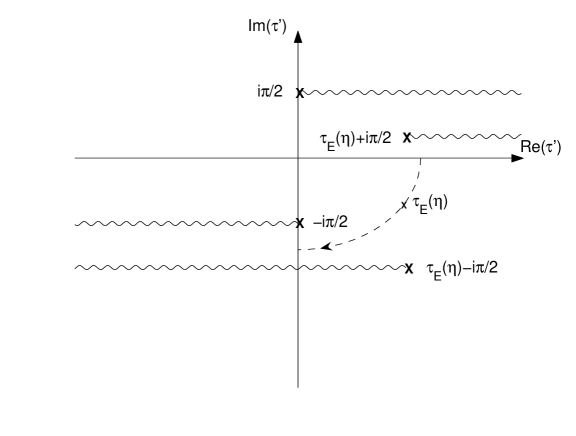
Figure 3: The branch cuts of the function $\cosh^{-\Delta_{1}}(\tau^{\prime}-\tau_{E}(\eta))\cosh^{-\Delta_{2}}(\tau^{\prime})$ during the $\tau_{E}$ rotation. The dashed curve shows the trajectory followed by the point $\tau_{E}(\eta)$, and the branch cuts are drawn for a particular point on this trajectory.

The way to perform this rotation depends on the value of $\tau$. We analyze 2 cases :

Case 1) $\tau<\pi$ : In this case we can choose the integration contour while rotating $\tau_{E}$ to be the contour parallel to the real axis at $i\frac{\textrm{Im}(\tau_{E}(\eta))}{2}$, ending up at the contour $\textrm{Im}(\tau^{\prime})=-\frac{i\tau}{2}$. After completing the rotation we end up with the integral (see figure 4):

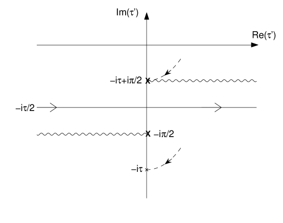
Figure 4: The $\tau^{\prime}$ contour after $\tau_{E}$ rotation for $0<\tau<\pi$. The relevant branch cuts of the function $\cosh^{-\Delta_{1}}(\tau^{\prime}+i\tau)\cosh^{-\Delta_{2}}(\tau^{\prime})$ are shown on the figure. The dashed curves show the last part of the trajectory followed by the points $\tau_{E}(\eta)$ and $\tau_{E}(\eta)+i\pi/2$ during the rotation.

$$G^{12}(\theta_{1}=0, \tau_{1}=\tau;\theta_{2}=0,\tau_{2}=0)=$$ (55)

$$hA\int_{-\infty}^{\infty}\cosh^{-\Delta_{1}}(\tau^{\prime}+i\frac{1}{2}\tau)\cosh^{-\Delta_{2}}(\tau^{\prime}-i\frac{1}{2}\tau)d\tau^{\prime},$$ (56)

the complex conjugate of which is (see appendix B):

$$(G^{12})^{*} =hA\int_{-\infty}^{\infty}\cosh^{-\Delta_{1}}(\tau^{\prime}-i\frac{1}{2}\tau)\cosh^{-\Delta_{2}}(\tau^{\prime}+i\frac{1}{2}\tau)d\tau^{\prime}=$$ (57)

$$=hA\int_{-\infty}^{\infty}\cosh^{-\Delta_{1}}(-\tau^{\prime}+i\frac{1}{2}\tau)\cosh^{-\Delta_{2}}(-\tau^{\prime}-i\frac{1}{2}\tau)d\tau^{\prime}=$$ (58)

$$=hA\int_{-\infty}^{\infty}\cosh^{-\Delta_{1}}(\tau^{\prime}+i\frac{1}{2}\tau)\cosh^{-\Delta_{2}}(\tau^{\prime}-i\frac{1}{2}\tau)d\tau^{\prime}=G^{12}.$$ (59)

So, the first order correction to the commutator of the two fields vanishes in this case,

$$i\textrm{Im}(G^{12})=0.$$ (60)

This is consistent with our expectations, since in this case $x_{1}$ is not in the ‘boundary affected’ region.

Case 2) $\pi<\tau<2\pi$ :

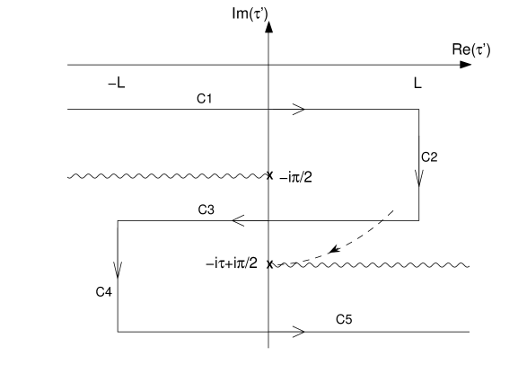
Figure 5: The $\tau^{\prime}$ contour after $\tau_{E}$ rotation for $\pi<\tau<2\pi$. The relevant branch cuts of the function $\cosh^{-\Delta_{1}}(\tau^{\prime}+i\tau)\cosh^{-\Delta_{2}}(\tau^{\prime})$ are shown on the figure. The dashed curve shows the last part of the trajectory followed by the point $\tau_{E}(\eta)+i\pi/2$ during the rotation.

In this case, in order to avoid the poles at $\tau^{\prime}=-i\frac{1}{2}\pi$ and $\tau^{\prime}=\tau_{E}(\eta)+i\frac{1}{2}\pi$, we need to deform the contour while rotating $\tau$. After the rotation is complete we end up with the contour shown in figure 5. Divide this contour into 5 straight contours: $C=C_{1}+C_{2}+C_{3}+C_{4}+C_{5}$ as shown in the figure,

$$C_{1}=(-\infty-i\frac{1}{2}\tau+i\frac{1}{2}\pi)\rightarrow(L-i\frac{1}{2}\tau+i\frac{1}{2}\pi)$$ (61)

$$C_{2}=(L-i\frac{1}{2}\tau+i\frac{1}{2}\pi)\rightarrow(L-i\frac{1}{2}\tau)$$ (62)

$$C_{3}=(L-i\frac{1}{2}\tau)\rightarrow(-L-i\frac{1}{2}\tau)$$ (63)

$$C_{4}=(-L-i\frac{1}{2}\tau)\rightarrow(-L-i\frac{1}{2}\tau-i\frac{1}{2}\pi)$$ (64)

$$C_{5}=(-L-i\frac{1}{2}\tau-i\frac{1}{2}\pi)\rightarrow(\infty-i\frac{1}{2}\tau-i\frac{1}{2}\pi)$$ (65)

where $L$ is some real positive number. The specific location and form of the contour were chosen for convenience.

By taking $L$ to infinity, the contribution of the sections $C_{2}$ and $C_{4}$ goes to zero and we end up with the union of

$$C_{1}=(-\infty-i\frac{1}{2}\tau+i\frac{1}{2}\pi)\rightarrow(\infty-i\frac{1}{2}\tau+i\frac{1}{2}\pi)$$ (66)

$$C_{3}=(\infty-i\frac{1}{2}\tau)\rightarrow(-\infty-i\frac{1}{2}\tau)$$ (67)

$$C_{5}=(-\infty-i\frac{1}{2}\tau-i\frac{1}{2}\pi)\rightarrow(\infty-i\frac{1}{2}\tau-i\frac{1}{2}\pi)$$ (68)

It is not hard to see that (see (133),(135))

$$\int_{C_{5}}=e^{i\pi(\Delta_{1}+\Delta_{2})}(\int_{C_{1}})^{*},$$ (69)

$$\int_{C_{3}}=e^{2\pi i(\Delta_{1}+\Delta_{2})}(\int_{C_{3}})^{*},$$ (70)

where $\int_{\gamma}$ stands for $\int_{\gamma}\cosh^{-\Delta_{1}}(\tau^{\prime}+i\tau)\cosh^{-\Delta_{2}}(\tau^{\prime})d\tau^{\prime}$. Thus, when $\Delta_{1}+\Delta_{2}=n$ for some integer even $n$, the sum of the integrals is real and the commutator is zero. However, for odd $n$ or for non-integer $\Delta_{1}+\Delta_{2}$ it is not zero in general. In particular there is a simple argument that it is not zero for $\tau\rightarrow\pi^{+}$. From (69) we can deduce that the phase of $\int_{C_{3}}$ is $\pi(\Delta_{1}+\Delta_{2})$ (up to addition of $\pi k$), $\int_{C_{3}}=\pm\left|\int_{C_{3}}\right|e^{i\pi(\Delta_{1}+\Delta_{2})}$. For general $\Delta_{1},\Delta_{2}$, for $\tau\rightarrow\pi^{+}$, the integrals $\int_{C_{1}}$ and $\int_{C_{5}}$ are finite, while the integral $\int_{C_{3}}$ goes to infinity. Since for $\Delta_{1}+\Delta_{2}$ non-integer the phase of $\int_{C_{3}}$ is not zero, the commutator which is its imaginary part goes to infinity as well. In particular it is not zero. This proves that the commutator of $\Phi_{1}$ and $\Phi_{2}$ does not vanish for the pairs of points we are interested in after the deformation (at least for specific values of $\tau$; we expect similar arguments to apply for any $\tau>\pi$).

4.2 Marginal deformation

A special case where we can compute the effect of the deformation (11) to all orders is the classically marginal case:

$$\Delta_{1}=d-\Delta_{2}\equiv\Delta.$$ (71)

Equation (71) means that $m_{1}^{2}=m^{2}_{2}\equiv m^{2}$, the only difference between the fields in the non-deformed case is their boundary condition. The fact that $\phi_{1}$ and $\phi_{2}$ have the same mass allows us to make the rotation:

$$\rho_{1}=\frac{1}{\sqrt{1+\tilde{h}^{2}}}(\phi_{1}+\tilde{h}\phi_{2}),~{}~{}~{}\rho_{2}=\frac{1}{\sqrt{1+\tilde{h}^{2}}}(-\tilde{h}\phi_{1}+\phi_{2}),$$ (72)

where $\tilde{h}=(2\Delta-d)h$. It is easy to show that if $\phi_{1}$ and $\phi_{2}$ satisfy the deformed boundary conditions (12) then the new fields, $\rho_{1}$ and $\rho_{2}$, satisfy the same bulk equations as $\phi_{1}$ and $\phi_{2}$ but have the undeformed boundary conditions, with $\rho_{1}$ behaving like a field dual to an operator with dimension $\Delta$ and $\rho_{2}$ with dimension $d-\Delta$. Since these are decoupled fields their propagator is trivial and we can substitute back to compute the propagator of $\phi_{1}$ and $\phi_{2}$ :

$$G_{E}^{ij}=\frac{1}{1+\tilde{h}^{2}}\left(\begin{array}[]{cc}G_{E\Delta}+\tilde{h}^{2}G_{E(d-\Delta)}&~{}~{}~{}~{}\tilde{h}G_{E\Delta}-\tilde{h}G_{E(d-\Delta)}\\ \tilde{h}G_{E\Delta}-\tilde{h}G_{E(d-\Delta)}&~{}~{}~{}~{}\tilde{h}^{2}G_{E\Delta}+G_{E(d-\Delta)}\end{array}\right).$$ (75)

To first order in $h$, there is only a correction to $G_{E}^{12}$,

$$G_{E}^{12}=\tilde{h}(G_{E\Delta}-G_{E(d-\Delta)}),$$ (76)

which can be shown to agree with (48).

5 Summary

In this paper we analyzed the effect of multi-trace deformations of the CFT on the bulk to bulk propagators of the corresponding $AdS_{d+1}\times M$ theory. We found that the resulting ‘bulk to bulk’ commutators of fields on $AdS_{d+1}\times M$ have a non-local property: they do not vanish for pairs of points in $AdS_{d+1}\times M$ that are connected by a space-like geodesic but not by a time-like geodesic (we would expect a commutator of fields to vanish at such points since the path integral over paths would be expected to be dominated by the space-like geodesic; these points are connected by a causal curve so the result does not violate causality). We showed that in a standard theory (with only single-trace deformations) the commutator of two scalar fields vanishes at any such pairs of points (at least for odd-dimensional AdS spaces). However, this is no longer true after deforming by multi-trace deformations (at least for the specific deformation we considered, and for specific choices of pairs of points, but we expect the result to be much more general).

Acknowledgements

We would like to thank T. Kashti, A. Patir, D. Reichmann and E. Silverstein for useful discussions. The work of OA and MB was supported in part by the Israel-U.S. Binational Science Foundation, by the Israel Science Foundation (grant number 1399/04), by the Braun-Roger-Siegl foundation, by the European network HPRN-CT-2000-00122, by a grant from the G.I.F., the German-Israeli Foundation for Scientific Research and Development, and by Minerva.

Appendix A Propagators in AdS space

In this appendix we will review some properties of the Feynman propagators in AdS space. The main result used in the text is the relation between the Feynman propagators in different space-time dimensions (100).

A.1 Propagator in Euclidean signature

Instead of working with the metric (3), we define a new radial coordinate $l$ by the geodesic distance from the origin, and then we can write the $EAdS_{d+1}$ metric as

$$ds^{2}=R^{2}(dl^{2}+\sinh^{2}(l)d\Omega_{d}^{2}).$$ (77)

The Laplacian in $EAdS_{d+1}$ in these coordinates is

$$\nabla^{2}\phi =\frac{1}{R^{2}}(R\sinh l)^{-d}\partial_{l}((R\sinh l)^{d}\partial_{l}\phi)+\frac{1}{R^{2}\sinh^{2}l}\nabla^{2}_{d}\phi=$$ (78)

$$=\frac{1}{R^{2}}\left(\partial_{l}^{2}+d\coth(l)\partial_{l}+\frac{1}{\sinh^{2}(l)}\nabla^{2}_{d}\right)\phi,$$ (79)

where $\nabla^{2}_{d}$ is the Laplacian on $S^{d}$. The Klein-Gordon (KG) equation, $(\nabla^{2}-m^{2})\phi=0$, in the case of spherical symmetry is:

$$\left(\partial_{l}^{2}+d\coth(l)\partial_{l}\right)\phi=R^{2}m^{2}\phi,$$ (80)

or:

$$f^{\prime\prime}+d\frac{c}{s}f^{\prime}=R^{2}m^{2}f,$$ (81)

where

$$\phi=f(l),$$ (82)

$$s\equiv\sinh(l),c\equiv\cosh(l),$$ (83)

$$f^{\prime}\equiv\partial_{l}f\Rightarrow c^{\prime}=s,~{}~{}~{}s^{\prime}=c.$$ (84)

Suppose we have a solution $f$ to equation (81). Define

$$g=f^{\prime}/s\Leftrightarrow f^{\prime}=sg\Rightarrow f^{\prime\prime}=cg+sg^{\prime}.$$ (85)

Plug this in (81):

$$sg^{\prime}+(d+1)cg=R^{2}m^{2}f\Rightarrow$$ (86)

$$sg^{\prime\prime}+(d+1)sg+(d+2)cg^{\prime}=R^{2}m^{2}sg\Rightarrow$$ (87)

$$g^{\prime\prime}+(d+2)\frac{c}{s}g^{\prime}=R^{2}(m^{2}-\frac{(d+1)}{R^{2}})g.$$ (88)

So, $g$ is a solution to (81) in $EAdS_{d+3}$ with mass

$$m_{d+2}^{2}=m_{d}^{2}-\frac{(d+1)}{R^{2}}.$$ (89)

Note that (89) means (using (4)):

$$\Delta_{d+2}-\frac{1}{2}(d+2)=\sqrt{(\frac{1}{2}(d+2))^{2}+m_{d+2}^{2}R^{2}}=\sqrt{(\frac{1}{2}d)^{2}+R^{2}m_{d}^{2}}=\Delta_{d}-\frac{1}{2}d.$$ (90)

So, if $\phi_{d}$ is a spherically symmetric solution to the KG equation in $EAdS_{d+1}$ corresponding to dimension $\Delta_{d}$, then $\phi_{d+2}$ defined as:

$$\phi_{d+2}(l)=\frac{1}{\sinh(l)}\frac{d}{dl}\phi_{d}$$ (91)

is a spherically symmetric solution to the KG equation in $EAdS_{d+3}$ corresponding to a conformal dimension $\Delta_{d+2}=\Delta_{d}+1$. The propagator is the solution to the KG equation for $l>0$ with the large $l$ behavior:

$$\phi_{d}(l)\propto e^{-\Delta_{d}l}.$$ (92)

By using (91) we see that $\phi_{d+2}$ has the same behavior as $\phi_{d}$, with $\Delta_{d+2}$. We conclude that the propagators in dimensions $d+1$ and $d+3$ are related:

$$G_{EAdS_{d+3}}(l,\Delta)\propto\frac{1}{\sinh(l)}\frac{d}{dl}G_{EAdS_{d+1}}(l,\Delta-1).$$ (93)

To check that this works we can calculate the propagator for some low dimensions. For $d=0$, (81) has the solutions $e^{\pm mRl}=e^{\Delta_{\pm}l}=e^{\pm\Delta l}$. For any even $d$, we can get the relevant solution by recursion using (93). For the lowest odd dimension $AdS_{3}$ we get

$$G_{EAdS_{3}}(l)\propto\frac{e^{-(\Delta-1)l}}{\sinh(l)}.$$ (94)

We can calculate the normalization factor by the requirement that the propagator should approach the flat space propagator for $Rl<<R,1/m$. We get:

$$G_{EAdS_{3}}(l)=-\frac{1}{4\pi R}\frac{e^{-(\Delta-1)l}}{\sinh(l)},$$ (95)

in agreement with the literature [18].

A.2 Propagator in Lorentzian signature

It will be convenient to work in global coordinates $(\rho,\tau,\Omega_{d-1})$ with the metric

$$ds^{2}=R^{2}(-\cosh^{2}\rho~{}d\tau^{2}+d\rho^{2}+\sinh^{2}\rho~{}d\Omega_{d-1}^{2}).$$ (96)

The propagator in Lorentzian signature is expressed as an analytic continuation of the propagator in $EAdS$, as a function of $\tau_{E}$, back to real time $\tau=-i\tau_{E}$. This means rotating $\tau_{E}$ along the contour:

$$\tau_{E}(\eta)=e^{-i\eta}\tau,~{}~{}~{}~{}\eta:0\rightarrow\frac{1}{2}\pi.$$ (97)

For $\rho=0$, $l=\tau_{E}$, the expressions (95) are analytic functions of $\tau_{E}$ without any branch cuts, so the rotation can be done trivially and we get the Feynman propagator

$$G_{AdS_{3}}(x,0)=i\frac{1}{4\pi R}\frac{e^{i(\Delta-1)\tau}}{\sin\tau}.$$ (98)

Since the propagator is invariant under the isometries of AdS, it must be a function of the geodesic proper time $\mu$ between the two points (this is true for pairs of points that have a timelike geodesic connecting them, which are the pairs that interest us; assume that the first point has a larger $\tau$ so that the time ordering has no effect). Thus we get:

$$G_{AdS_{3}}(\mu;m^{2})=i\frac{1}{4\pi R}\frac{e^{i(\Delta-1)\frac{\mu}{R}}}{\sin\frac{\mu}{R}}=i\frac{1}{4\pi R}\frac{e^{i\mu\sqrt{m^{2}+\frac{1}{R^{2}}}}}{\sin\frac{\mu}{R}}.$$ (99)

Similarly, by analytically continuing (93) we get

$$G_{AdS_{d+3}}(\mu,m^{2})\propto\frac{1}{\sin(\frac{\mu}{R})}\frac{d}{d\mu}G_{AdS_{d+1}}(\mu,m^{2}+\frac{d+1}{R^{2}}).$$ (100)

Appendix B Properties of the function $\cosh^{-\Delta_{1}}(\tau^{\prime}-\tau)\cosh^{-\Delta_{2}}(\tau^{\prime})$

B.1 Properties of $\cosh^{\alpha}(z)$

The function $\cosh(z)$ has zeros at $z=i\frac{1}{2}\pi+i\pi k$ for integer $k$. Define the branch cut of the function $z^{\alpha}$ to be at $(0+0i,0+i\infty)$. This means we write

$$z^{\alpha}\equiv\left|z\right|^{\alpha}e^{i\sigma\alpha},~{}~{}\textrm{where}~{}~{}z=\left|z\right|e^{i\sigma}~{}~{}\textrm{with}~{}~{}-\frac{3}{2}\pi<\sigma\leq\frac{1}{2}\pi.$$ (101)

With this choice the function $\cosh^{\alpha}(z)$ has branch cuts along the half-lines $(\textrm{Im}(z)=\frac{1}{2}\pi+2\pi k,\textrm{Re}(z)>0)$ and $(\textrm{Im}(z)=-\frac{1}{2}\pi+2\pi k,\textrm{Re}(z)<0)$ (see figure 6 for the first few branch cuts).

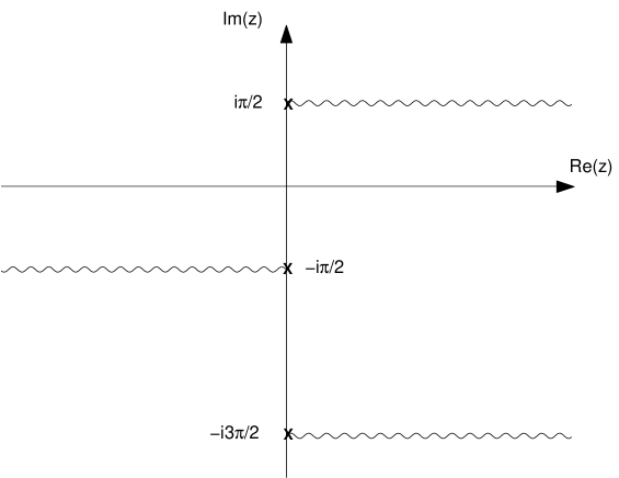
Figure 6: The branch cuts of the function $\cosh^{\alpha}(z)$

Note that with the definition (101)

$$(z^{\alpha})^{*}=\left\{\begin{array}[]{cc}(z^{*})^{\alpha}&-\frac{1}{2}\pi\leq\sigma\leq\frac{1}{2}\pi\\ e^{2\pi i\alpha}(z^{*})^{\alpha}&-\frac{3}{2}\pi<\sigma<-\frac{1}{2}\pi\\ \end{array}\right.$$ (104)

$$(-z)^{\alpha}=\left\{\begin{array}[]{cc}e^{-i\pi\alpha}z^{\alpha}&-\frac{1}{2}\pi\leq\sigma\leq\frac{1}{2}\pi\\ e^{i\pi\alpha}z^{\alpha}&-\frac{3}{2}\pi<\sigma<-\frac{1}{2}\pi\\ \end{array}\right.$$ (107)

The function $\cosh(z)$ with $z=\textrm{Re}(z)+i\textrm{Im}(z)$ obeys

$$\cosh(z)=\cosh(\textrm{Re}(z))\cos(\textrm{Im}(z))+i\sinh(\textrm{Re}(z))\sin(\textrm{Im}(z)).$$ (108)

Note that for

$$\cosh(z)=\left|\cosh(z)\right|e^{i\sigma}~{}~{}\textrm{with}~{}~{}-\frac{3}{2}\pi<\sigma\leq\frac{1}{2}\pi$$ (109)

we find that (up to $z\rightarrow z+2\pi ik$)

$$-\frac{1}{2}\pi\leq\sigma\leq\frac{1}{2}\pi\Leftrightarrow-\frac{1}{2}\pi\leq\textrm{Im}(z)\leq\frac{1}{2}\pi$$ (110)

$$-\frac{3}{2}\pi<\sigma<-\frac{1}{2}\pi\Leftrightarrow-\frac{3}{2}\pi<\textrm{Im}(z)<-\frac{1}{2}\pi,$$ (111)

so

$$(\cosh(z)^{\alpha})^{*}=\left\{\begin{array}[]{cc}\cosh^{\alpha}(z^{*})&-\frac{1}{2}\pi\leq\textrm{Im}(z)\leq\frac{1}{2}\pi\\ e^{2\pi i\alpha}\cosh^{\alpha}(z^{*})&-\frac{3}{2}\pi<\textrm{Im}(z)<-\frac{1}{2}\pi\\ \end{array}\right.$$ (114)

$$(-\cosh(z))^{\alpha}=\left\{\begin{array}[]{cc}e^{-i\pi\alpha}\cosh^{\alpha}(z)&-\frac{1}{2}\pi\leq\textrm{Im}(z)\leq\frac{1}{2}\pi\\ e^{i\pi\alpha}\cosh^{\alpha}(z)&-\frac{3}{2}\pi<\textrm{Im}(z)<-\frac{1}{2}\pi.\\ \end{array}\right.$$ (117)

To summarize, the poles and branch cuts of $\cosh^{\alpha}(z)$ are :

$$\cosh(z) =0\Leftrightarrow\textrm{Re}(z)=0,\textrm{Im}(z)=\frac{1}{2}\pi+\pi k,$$ (118)

$$\cosh(z) \in(0+i0,0+i\infty)\Leftrightarrow$$ (119)

$$(\textrm{Im}(z)=\frac{1}{2}\pi+2\pi k,~{}\textrm{Re}(z)>0)~{}\textrm{or}~{}(\textrm{Im}(z)=-\frac{1}{2}\pi+2\pi k,~{}\textrm{Re}(z)<0).$$ (120)

B.2 Derivation of equation (4.14)

Divide each contour into two parts (-infinity to zero and zero to infinity) :

$$C_{1a}=(-\infty-i\frac{1}{2}\tau+i\frac{1}{2}\pi)\rightarrow(0-i\frac{1}{2}\tau+i\frac{1}{2}\pi)$$ (121)

$$C_{1b}=(0-i\frac{1}{2}\tau+i\frac{1}{2}\pi)\rightarrow(\infty-i\frac{1}{2}\tau+i\frac{1}{2}\pi)$$ (122)

$$C_{3a}=(\infty-i\frac{1}{2}\tau)\rightarrow(0-i\frac{1}{2}\tau)~{}~{}~{}C_{3b}=(0-i\frac{1}{2}\tau)\rightarrow(-\infty-i\frac{1}{2}\tau)$$ (123)

$$C_{5a}=(-\infty-i\frac{1}{2}\tau-i\frac{1}{2}\pi)\rightarrow(0-i\frac{1}{2}\tau-i\frac{1}{2}\pi)$$ (124)

$$C_{5b}=(0-i\frac{1}{2}\tau-i\frac{1}{2}\pi)\rightarrow(\infty-i\frac{1}{2}\tau-i\frac{1}{2}\pi)$$ (125)

Note that:

$$(\int_{C_{1a}})^{*}=e^{-2\pi i\Delta_{1}}\int_{-\infty}^{0}\cosh^{-\Delta_{1}}(\tau^{\prime}-i\frac{1}{2}\tau-i\frac{1}{2}\pi)\cosh^{-\Delta_{2}}(\tau^{\prime}+i\frac{1}{2}\tau-i\frac{1}{2}\pi)d\tau^{\prime}=$$ (126)

$$=e^{-2\pi i\Delta_{1}}\int^{\infty}_{0}\cosh^{-\Delta_{1}}(\tau^{\prime}+i\frac{1}{2}\tau+i\frac{1}{2}\pi)\cosh^{-\Delta_{2}}(\tau^{\prime}-i\frac{1}{2}\tau+i\frac{1}{2}\pi)d\tau^{\prime}=$$ (127)

$$=e^{-2\pi i\Delta_{1}}\int_{C_{1b}}=$$ (128)

$$=e^{-2\pi i\Delta_{1}}e^{+i\pi\Delta_{1}}e^{-i\pi\Delta_{2}}\int^{\infty}_{0}\cosh^{-\Delta_{1}}(\tau^{\prime}+i\frac{1}{2}\tau-i\frac{1}{2}\pi)\cosh^{-\Delta_{2}}(\tau^{\prime}-i\frac{1}{2}\tau-i\frac{1}{2}\pi)d\tau^{\prime}=$$ (129)

$$=e^{-i\pi(\Delta_{1}+\Delta_{2})}\int_{C_{5b}},$$ (130)

where in the last line, we used the relation $\cosh(z\pm i\pi)=-\cosh(z)$.

Using similar relations we find:

$$\int_{C_{5a}}=e^{i\pi(\Delta_{2}-\Delta_{1})}\int_{C_{1a}}=e^{i\pi(\Delta_{1}+\Delta_{2})}(\int_{C_{1b}})^{*}$$ (131)

$$\int_{C_{3b}}=e^{2\pi i(\Delta_{1}+\Delta_{2})}(\int_{C_{3a}})^{*}.$$ (132)

Thus,

$$\int_{C_{5}} =\int_{C_{5a}}+\int_{C_{5b}}=e^{i\pi(\Delta_{1}+\Delta_{2})}(\int_{C_{1b}})^{*}+e^{i\pi(\Delta_{1}+\Delta_{2})}(\int_{C_{1a}})^{*}=$$ (133)

$$=e^{i\pi(\Delta_{1}+\Delta_{2})}(\int_{C_{1}})^{*}$$ (134)

and

$$\int_{C_{3}} =\int_{C_{3a}}+\int_{C_{3b}}=e^{2\pi i(\Delta_{1}+\Delta_{2})}(\int_{C_{3b}})^{*}+e^{2\pi i(\Delta_{1}+\Delta_{2})}(\int_{C_{3a}})^{*}=$$ (135)

$$=e^{2\pi i(\Delta_{1}+\Delta_{2})}(\int_{C_{3}})^{*}.$$ (136)

References

- [1] J. M. Maldacena, “The large N limit of superconformal field theories and supergravity,” Adv. Theor. Math. Phys. 2, 231 (1998) [Int. J. Theor. Phys. 38, 1113 (1999)] [arXiv:hep-th/9711200].
- [2] S. S. Gubser, I. R. Klebanov and A. M. Polyakov, “Gauge theory correlators from non-critical string theory,” Phys. Lett. B 428, 105 (1998) [arXiv:hep-th/9802109].
- [3] E. Witten, “Anti-de Sitter space and holography,” Adv. Theor. Math. Phys. 2, 253 (1998) [arXiv:hep-th/9802150].
- [4] G. T. Horowitz and N. Itzhaki, “Black holes, shock waves, and causality in the AdS/CFT correspondence,” JHEP 9902 (1999) 010 [arXiv:hep-th/9901012].
- [5] D. Kabat and G. Lifschytz, “Gauge theory origins of supergravity causal structure,” JHEP 9905, 005 (1999) [arXiv:hep-th/9902073].
- [6] J. P. Gregory and S. F. Ross, “Looking for event horizons using UV/IR relations,” Phys. Rev. D 63 (2001) 104023 [arXiv:hep-th/0012135].
- [7] V. E. Hubeny, M. Rangamani and S. F. Ross, “Causal structures and holography,” arXiv:hep-th/0504034.
- [8] O. Aharony, M. Berkooz and E. Silverstein, “Multiple-trace operators and non-local string theories,” JHEP 0108 (2001) 006 [arXiv:hep-th/0105309].
- [9] E. Witten, “Multi-trace operators, boundary conditions, and AdS/CFT correspondence,” arXiv:hep-th/0112258.
- [10] M. Berkooz, A. Sever and A. Shomer, “Double-trace deformations, boundary conditions and spacetime singularities,” JHEP 0205, 034 (2002) [arXiv:hep-th/0112264].
- [11] A. Sever and A. Shomer, “A note on multi-trace deformations and AdS/CFT,” JHEP 0207, 027 (2002) [arXiv:hep-th/0203168].
- [12] O. Aharony, M. Berkooz and E. Silverstein, “Non-local string theories on and stable non-supersymmetric backgrounds,” Phys. Rev. D 65 (2002) 106007 [arXiv:hep-th/0112178].
- [13] I. R. Klebanov and E. Witten, “AdS/CFT correspondence and symmetry breaking,” Nucl. Phys. B 556, 89 (1999) [arXiv:hep-th/9905104].
- [14] W. Muck, “An improved correspondence formula for AdS/CFT with multi-trace operators,” Phys. Lett. B 531, 301 (2002) [arXiv:hep-th/0201100].
- [15] S. S. Gubser and I. R. Klebanov, “A universal result on central charges in the presence of double-trace deformations,” Nucl. Phys. B 656, 23 (2003) [arXiv:hep-th/0212138].
- [16] P. Minces, “Multi-trace operators and the generalized AdS/CFT prescription,” Phys. Rev. D 68, 024027 (2003) [arXiv:hep-th/0201172].
- [17] P. Breitenlohner and D. Z. Freedman, “Stability In Gauged Extended Supergravity,” Annals Phys. 144, 249 (1982).
- [18] T. Inami and H. Ooguri, “One Loop Effective Potential In Anti-De Sitter Space,” Prog. Theor. Phys. 73, 1051 (1985).