hep-th/0504176

RIKEN-TH-40

Localization on the D-brane, two-dimensional gauge theory and matrix models

So Matsuura and Kazutoshi Ohta

Theoretical Physics Laboratory
The Institute of Physical and Chemical Research (RIKEN)
2-1 Hirosawa, Wako
Saitama 351-0198, JAPAN

Abstract

We consider the effective topological field theory on Euclidean D-strings wrapping on a 2-cycle in the internal space. We evaluate the vev of a suitable operator corresponding to the chemical potential of vortices bounded to the D-strings, and find that it reduces to the partition function of generalized two-dimensional Yang-Mills theory as a result of localization. We argue that the partition function gives a grand canonical ensemble of multi-instanton corrections for four-dimensional ${\cal N}{=}2$ gauge theory in a suitable large $N$ limit. We find two-dimensional gauge theories that provide the instanton partition function for four-dimensional ${\cal N}{=}2$ theories with the hypermultiplets in the adjoint and fundamental representations. We also propose a partition function that gives the instanton contributions to four-dimensional ${\cal N}{=}2$ quiver gauge theory. We discuss the relation between Nekrasov’s instanton partition function and the Dijkgraaf-Vafa theory in terms of large $N$ phase transitions of the generalized two-dimensional Yang-Mills theory.

1 Introduction and Summary

One of the most significant developments in supersymmetric (SUSY) gauge theories in recent years is that non-perturbative dynamics including instanton corrections becomes to be captured by interesting physical/mathematical systems. In particular, the prepotential of four-dimensional ${\cal N}{=}2$ SUSY gauge theory and the superpotential of ${\cal N}{=}1$ SUSY gauge theory, which are both holomorphic, are obtained from the free energy of a random partition [1] and a random matrix model [2, 3, 4], respectively. It is also pointed out that the random partition describing the prepotential of the ${\cal N}{=}2$ theory is related to a large $N$ limit of two-dimensional Yang-Mills theory [5]. Similar developments have also come to topological string theories. For example, amplitudes on a singular Calabi-Yau manifold are obtained from some statistical model like the melting crystal [6, 7]. Furthermore, the closed topological string amplitude also has a dual open string picture which is described by the large $N$ limit of three-dimensional Chern-Simons gauge theory [8, 9].

An interesting fact is that these systems are “bosonic” even though the original gauge theories and the topological string theories are preserving SUSY. In prior to the discovery of the relationship between the holomorphic quantities of the SUSY systems and the bosonic partition functions, relations between SUSY gauge theories and “bosonic” integrable systems are already pointed out (see for review [10]). In fact, the Seiberg-Witten curve of the four-dimensional ${\cal N}{=}2$ SUSY gauge theory is especially the spectrum curve for the integrable system and vacua in the four-dimensional ${\cal N}{=}1$ theory are equilibrium points of the related integrable system [11].

The key to understand these relations should exist in a localization of the path integral in an effective theory on D-branes. The non-perturbative corrections to the SUSY gauge theory are coming from corrections of Euclidean BPS D-branes, whose world-volume does not contain the time direction and which are wrapping on non-trivial cycles in an internal space, if we embed the gauge theory into a string theoretical configuration with a suitable compactification. According to [12], the effective theory on the Euclidean D-brane must be topologically twisted. Moreover, if we use the feature of the topological field theory, the partition function is reduced to a “bosonic” system after integrating out all fermionic fields due to the localization [13, 14].

In this paper, we discuss the relation between SUSY gauge theories and two-dimensional (bosonic) gauge theories from the first principle, that is, from the view point of the localization. We first give a configuration of D-branes that realize an ${\cal N}{=}2$ SUSY gauge theory and consider the effective theory on the D-branes wrapping on the internal 2-cycle in section 2. We evaluate the expectation value of an operator, which corresponds to the chemical potential of vortices on the cycle, and show that it reduces to the BF-theory. If we deform generically the D-brane effective theory by adding a “potential” term, we obtain the partition function of the so-called generalized two-dimensional Yang-Mills (${{\rm gYM}_{2}}$) theory [15, 16]. This reduction is essential reason why the prepotential of the SUSY gauge theory and the partition function of the two-dimensional Yang-Mills theory are related with each other. In this section, we also discuss the relation between our analysis and the argument given in [17, 18] where the authors derive the $q$-deformed two-dimensional Yang-Mills theory using a similar setup.

Moreover, in section 3, we proceed the path integral of ${{\rm gYM}_{2}}$ following the standard gauge theoretical method [19, 20]. We will see that the system finally reduces to a “discrete matrix model”. The difference between the discrete matrix model and an ordinary random matrix model, which is a model for $c{=}0$ string theory and effective superpotential calculations by Dijkgraaf and Vafa, is that eigenvalues of the discrete matrix model are discretized in a unit while the eigenvalues of the ordinary matrix model are continuous variables. Each eigenvalue can not exist at the same position (value) due to the existence of the Vandermonde determinant. So a possible set of eigenvalues is given by a strongly decreasing (non-colliding) integer sequence. Thus the integral over possible eigenvalues in the partition function of the random matrix model is replaced by a summation over possible sets of non-colliding ordered integers. On the other hand, if we map these discrete eigenvalue distributions to a weakly decreasing sequence by a suitable shift, we can identify the integer sequence with numbers of rows of a Young diagram. Using this identification, we can see the relation between the discrete matrix model and Migdal’s partition function [21], which is expressed as a summation over sets of the Young diagrams (representations of $U(N)$). In addition, we regard the eigenvalues as states of free fermions obeying the exclusion principle by using the famous Young diagram/Maya diagram (free fermion states) correspondence [22].

We find that the discrete matrix model possesses an essential structure of Nekrasov’s instanton partition function. If we consider a potential term, the eigenvalues of the discrete matrix model are accumulated around the critical points of the potential, then each lump of the eigenvalues has two end points (fermi surfaces). We show that a suitable large $N$ limit decouples these fermi surfaces with each other. Then the partition function is factorized into two sectors, and one of them produces the instanton partition function whose rank of the gauge group and moduli parameters of ${\cal N}{=}2$ theory are determined by the critical points of the ${{\rm gYM}_{2}}$ potential. This manner to take the large $N$ limit is similar to the chiral decomposition by Gross and Taylor [23, 24, 25] (and see for review [26]).

In section 4, we extend the arguments in section 3 to the ${\cal N}{=}2$ theories including the hypermultiplets in various representations. We first derive Nekrasov’s partition function of theory with the hypermultiplet in the adjoint representation given in [27, 1] from a suitable two-dimensional model. To obtain the initial two-dimensional theory, we add extra observables to the topological theory, and the additional terms have the same form as the (tree level) superpotential of the corresponding four-dimensional theory. This extension very looks like the Dijkgraaf-Vafa’s construction to determine the matrix model actions, which is simply obtained from the tree level superpotential by replacing the superfields with the hermitian matrices. Then we get Nekrasov’s partition function of this model from the large $N$ limit again. Once we obtain the manner to make the observables for adjoint matters, it is easy to generalize it to the quiver theory and the theory with the hypermultiplets in the fundamental representation, since these theories are essentially reproduced by flows from the theory with the adjoint matter. We exhibit an $U(r)\times U(s)$ $A_{2}$-type quiver theory and an $U(r)$ gauge theory with $s$ flavors in the fundamental representation.

In section 5, we discuss the relationship between the discrete matrix model and usual continuous matrix model more explicitly. There we see the discrete matrix model in the continuum and large $N$ limit has two different type of third order phase transitions. One is called as the Douglas-Kazakov phase transition [29] and another is the Gross-Witten phase transition [30]. We give a correspondence between the limiting shape of the Young diagram and the eigenvalue density (free fermion states). We find that the Douglas-Kazakov and Gross-Witten phase transition are dual under electron/hall exchanges (exchanges of the eigenvalue and vacant positions). Combining these observations with the arguments in section 3, we also find the continuum and large $N$ limit to derive the Nekrasov’s instanton partition function and Dijkgraaf-Vafa’s matrix model analysis should lie on different phases of the discrete matrix model. We expect that relations among various phases may connect non-perturbative dynamics of ${\cal N}{=}2$ and ${\cal N}{=}1$ theories.

2 Localization on D-brane and two-dimensional YM theory

Four-dimensional gauge theories with eight supercharges can be realized in string theory in various ways like the geometric engineering [31, 32] and Hanany-Witten type brane configuration [33, 34]. Among them, we consider Type IIB superstring theory on $\mathbb{R}^{1,3}\times\mathbb{C}\times{\cal M}_{4}$, where ${\cal M}_{4}$ is a four-dimensional ALE space. If D5-branes are wrapped on 2-cycles in ${\cal M}_{4}$, a four-dimensional gauge theory will appear on the extra $\mathbb{R}^{1,3}$ space on the D5-branes except for the compactified internal 2-cycles. The configuration for the four-dimensional gauge theory preserves 8 supercharges at least when the 2-cycle is $\mathbb{C}{\rm P}^{1}$, which is T-dual to the Hanany-Witten Type IIA brane configuration of the four-dimensional ${\cal N}{=}2$ SUSY gauge theory. So it is sufficient to consider the case of $\mathbb{C}{\rm P}^{1}$ from the field theoretical point of view, but we will treat genus of the 2-cycle as generic one throughout the paper. So we assume the structure near a single cycle is $T^{*}\Sigma_{G}$, where $\Sigma_{G}$ is a Riemann surface with genus $G$, that is, the world-volume of the D5-branes is thought to be spanned along $\mathbb{R}^{1,3}\times\Sigma_{G}$. The gauge coupling of the four-dimensional system relates to the area $A$ of $\Sigma_{G}$ by

$$\frac{1}{g_{\rm YM_{4}}^{2}}=\frac{A}{g_{s}l_{s}^{2}}.$$ (2.1)

We set $l_{s}=1$ hereafter.

In this article, we are interested in contribution of instantons to the partition function of the four-dimensional ${\cal N}{=}2$ SUSY gauge theory. To this end, we start from the worldvolume theory of D5-branes on $\mathbb{R}^{1,3}\times\Sigma_{G}$ described above. It is known that the theory admits noncommutative deformation on $\mathbb{R}^{1,3}$ and it does not affect to the final result of the prepotential [35, 36]. According to the concept of the large $N$ reduction due to the noncommutativity [37, 38, 39], the worldvolume theory on D5-branes is reduced to the two-dimensional gauge theory on a large number of Euclidean D-strings wrapping on $\Sigma_{G}$. As discussed in [12], the low energy effective theory on D-branes wrapping on the cycle must be (partially) topologically twisted to preserve the SUSY. In this case, the topological theory should be localized on the Hitchin system,

$$F_{z\bar{z}}=\left[W_{z},\overline{W}_{\bar{z}}\right],\qquad\overline{D}_{\bar{z}}W_{z}=D_{z}\overline{W}_{\bar{z}}=0\,,$$ (2.2)

where $W_{z}$ and $\overline{W}_{\bar{z}}$ are 1-forms on $\Sigma_{G}$ associated with the normal bundle of $\Sigma_{G}$. Notice that these fields correspond to the fluctuation of $\Sigma_{G}$ in ${\cal M}_{4}$. However, we can simplify the analysis by giving a huge mass to $W_{z}$ [17]. Correspondingly, we freeze the degrees of freedom as $W_{z}=\overline{W}_{\bar{z}}=0$ and the system is localized on the flat connection $F=0$.

The twisted theory on the internal cycles enjoys the BRST symmetry and contains essentially a two-dimensional gauge field $A\equiv A_{i}dx^{i}$ ($i=1,2$), its (fermionic) BRST partner $\lambda\equiv\lambda_{i}dx^{i}$ and a complex scalar field $\Phi$ in the adjoint representation of the gauge group $U(N)$ which corresponds to the position of D-strings in the flat directions $\mathbb{C}$. These fields transform under the BRST symmetry as

$$QA=\lambda,\quad Q\lambda=-d_{A}\Phi,\quad Q\Phi=0,$$ (2.3)

where $d_{A}\Phi\equiv d\Phi+\left[A,\Phi\right]$. The BRST operator $Q$ is nilpotent up to the gauge transformation, and $A$, $\lambda$ and $\Phi$ have the ghost (BRST) charges of 0,1 and 2, respectively. As mentioned above, we need to impose the condition $F\equiv dA+A\wedge A=0$. To make this constraint and write down Lagrangian, we need additional BRST multiplets $(\bar{\Phi},\eta)$ and $(H,\chi)$, which transform as

$$\begin{array}[]{ll}Q\bar{\Phi}=\eta,&Q\eta=[\Phi,\bar{\Phi}],\\ QH=[\Phi,\chi],&Q\chi=H.\end{array}$$ (2.4)

Using these BRST multiplets, the action of the twisted theory can be written in the BRST exact form as

$$S_{\rm top}=\frac{1}{h^{2}}Q\int_{\Sigma_{G}}{\rm Tr}\,\Xi(A,\lambda,\Phi,\bar{\Phi},\eta,H,\chi),$$ (2.5)

where $h^{2}$ is a coupling constant which is proportional to the string coupling $g_{s}$ and

$$\Xi=\frac{1}{4}\eta[\Phi,\bar{\Phi}]+\frac{1}{2}\chi(H-2\ast F)+d_{A}\bar{\Phi}\wedge\lambda.$$ (2.6)

If we write the bosonic and fermionic fields together as $\vec{\cal B}=(A,H,\bar{\Phi})$ and $\vec{\cal F}=(\lambda,\chi,\eta)$, respectively (note that $\Phi$ does not have any fermionic partner), the partition function is given by a path integral over these fields;

$$Z_{\rm top}=\int{\cal D}\vec{\cal B}{\cal D}\vec{\cal F}{\cal D}\Phi e^{-\frac{1}{h^{2}}Q\int_{\Sigma_{G}}{\rm Tr}\,\Xi(\vec{\cal B},\vec{\cal F},\Phi)}.$$ (2.7)

Here we notice that the action (2.5) can be obtained from the dimensional or large $N$ reduction from the four-dimensional twisted ${\cal N}{=}2$ gauge theory, where an adjoint scalar field and a Lagrange multiplier corresponding to the moduli and constraints of the normal direction to the 2-cycle are thrown away by turning on a huge mass [40].

From the variation of the partition function with respect to the coupling constant $h^{2}$, we find the partition function (2.7) is independent of the coupling. This means that the path integral can be evaluated exactly in the WKB (weak coupling) limit. So the path integral dominates around the Gaussian integrals with the constraints. In particular, by integrating out $H$, this integral gives a flat connection constraint $F=0$. Therefore, any physical observables must be evaluated around the flat connections and the path integral (2.7) gives schematically the “volume” of the moduli space of the flat connections, namely the genus $G$ Riemann surface with marked points.

Next we consider BPS bound states on the D-strings. In the context of the topological field theory, we can introduce the chemical potentials for the BPS objects bounded on the D-strings by evaluating the vacuum expectation value of observables in the topological field theory [17]. In general, observables in topological field theory are cohomology classes of the BRST operator, which are constructed from $p$-forms ${\cal O}_{p}$ obeying the descent equations [40],

$$\begin{array}[]{l}d_{A}{\cal O}_{0}=Q{\cal O}_{1},\qquad d_{A}{\cal O}_{1}=Q{\cal O}_{2},\end{array}$$ (2.8)

where,

$$\begin{array}[]{l}{\cal O}_{0}=\frac{1}{2}{\rm Tr}\,\Phi^{2},\\ {\cal O}_{1}={\rm Tr}\,\Phi\lambda,\\ {\cal O}_{2}={\rm Tr}\,\left(i\Phi F+\frac{1}{2}\lambda\wedge\lambda\right).\end{array}$$ (2.9)

Let us first consider the integral of 2-form ${\cal O}_{2}$;

$$I_{2}(\Sigma_{G})=\int_{\Sigma_{G}}{\rm Tr}\,\left(i\Phi F+\frac{1}{2}\lambda\wedge\lambda\right),$$ (2.10)

and consider the vacuum expectation value,

$$\left\langle e^{-\frac{1}{g_{s}}I_{2}(\Sigma_{G})}\right\rangle_{\rm top}\equiv\int{\cal D}\vec{\cal B}{\cal D}\vec{\cal F}{\cal D}\Phi\exp\left\{\int_{\Sigma_{G}}{\rm Tr}\,\left[-\frac{1}{h^{2}}Q\Xi-\frac{1}{g_{s}}\left(i\Phi F+\lambda\wedge\lambda\right)\right]\right\},$$ (2.11)

in the topological field theory discussed above. This observable corresponds to the chemical potential of vortices on the D-strings. In fact, in the next section, we will show that $I_{2}(\Sigma_{G})$ introduces a coupling of the eigenvalues of $\Phi$ with the instanton numbers corresponding to the maximally broken gauge symmetry $U(1)^{N}$. The localization onto the moduli space of the flat connection due to the topological action does not affect to the physical part of the action $\frac{1}{g_{s}}\int_{\Sigma_{G}}\left(i\Phi F+\lambda\wedge\lambda\right)$, since the e.o.m. of the BF-theory also gives the flat connection constraint $F=0$. So, after integrating out the bilinear of $\lambda$, we find (2.11) exactly reduces to a partition function of the bosonic BF theory [13],

$$\left\langle e^{-\frac{1}{g_{s}}I_{2}(\Sigma_{G})}\right\rangle_{\rm top}=\int{\cal D}A{\cal D}\Phi\exp\left[-\frac{1}{g_{s}}\int_{\Sigma_{G}}{\rm Tr}\,i\Phi F\right].$$ (2.12)

We can also consider zero-form observables in the topological field. Especially, we consider operators in the form of the trace of polynomials of $\Phi$, which are actuarially observables since $\Phi$ is BRST closed itself. Recall that $\Phi$ corresponds to the positions of D5-branes in the $\mathbb{C}$-direction, which are the moduli parameters of vacua in Coulomb phase of the four-dimensional theory. To fix the moduli parameters in the four-dimensional theory, we add a generic $(r+1)$-the order superpotential for the adjoint scalar field manually, then the moduli parameters are expected to be fixed around the critical points of the superpotential [2]. We can realize this procedure in the two-dimensional theory by deforming the expectation value (2.11) by the observable,

$${\rm Tr}\,W(\Phi)\equiv\sum_{j=1}^{r+1}\frac{\mu_{j}}{j}{\rm Tr}\,\Phi^{j}.$$ (2.13)

In contrast to the previous case without potential, we cannot claim that the expectation value of the observable deformed by the potential, $I_{2}(\Sigma_{G})+\int_{\Sigma_{G}}{\rm Tr}\,W(\Phi)\omega$ (where $\omega$ is a volume form on $\Sigma_{G}$), is the same as the partition function of the deformed BF theory, since higher critical points corresponding to $F\neq 0$ may contribute to the path integral. However, as discussed in [13], the contributions from the higher critical points are exponentially small. Thus, after integrating out $\lambda$, we can again evaluate approximately the expectation value in the topological field theory as the partition function of a “physical” theory up to the contribution from the higher critical points;

$$\left\langle\exp\left[-\frac{1}{g_{s}}\int_{\Sigma_{G}}{\rm Tr}\,\left(i\Phi F+\lambda\wedge\lambda\right)-\frac{1}{g_{s}}\int_{\Sigma_{G}}{\rm Tr}\,W(\Phi)\omega\right]\right\rangle_{\rm top}\\ \cong\int{\cal D}A{\cal D}\Phi\exp\left[-\frac{1}{g_{s}}\int_{\Sigma_{G}}{\rm Tr}\,\Bigl{(}i\Phi F+W(\Phi)\omega\Bigr{)}\right].$$ (2.14)

Fortunately, however, the e.o.m of the r.h.s. theory with respect to $\Phi$ gives

$$iF=W^{\prime}(\Phi)\omega.$$ (2.15)

So we can expect that the above approximation becomes much better, if we take into account configurations only around the critical points $W^{\prime}=0$, where the contribution from the flat connection $F=0$ is dominated.

Hereafter we investigate the bosonic BF type theory deformed by the potential as an effective theory of the D-strings with vortices. This model is known as the generalized two-dimensional Yang-Mills theory (${{\rm gYM}_{2}}$) [15], which is a generalization of the ordinary two-dimensional $U(N)$ Yang-Mills theory. Indeed, if we choose a quadratic potential $W(\Phi)=\frac{\mu_{2}}{2}\Phi^{2}$, the above partition function reduces to the usual two-dimensional Yang-Mills theory after integrating out $\Phi$,

$$Z_{\rm YM_{2}}=\int{\cal D}A\exp\left[-\frac{1}{2g_{\rm YM_{2}}^{2}}\int d^{2}x{\rm Tr}\,F^{2}\right],$$ (2.16)

with an identification of $g_{\rm YM_{2}}=g_{s}\mu_{2}$.

Before closing this section, we need to mention on the relationship between our model and a system argued in [18]. In the context of [18], the adjoint scalar $\Phi$ comes from the holonomy of the gauge field at infinity of a fiber direction, which causes the periodicity of the field $\Phi\sim\Phi+2\pi$. Then one needs to use a unitary measure for it and the model gets the $q$-deformation. On the other hand, in our model, we do not assume such a periodicity in the $\mathbb{C}$-direction, which is associated with the vev for the adjoint scalar field $\Phi$. Namely, a range of value of $\Phi$ is non-compact and we do not need to use the unitary measure. In other words, our model is thought to be a decompacified limit of the periodic direction in the fiber. So we have the ${{\rm gYM}_{2}}$, not the $q$-deformed one.

3 Instanton counting from two-dimensional gauge theory

3.1 Migdal’s partition function (Gaussian model)

In prior to investigating the partition function of the ${{\rm gYM}_{2}}$, we derive Migdal’s partition function [21] for the ordinary two-dimensional Yang-Mills theory by using the Abelianization technique developed in [19, 20]. As mentioned in the previous section, the partition function of the two-dimensional Yang-Mills theory can be written as the ${{\rm gYM}_{2}}$ with the quadratic potential,

$$Z=\int{\cal D}A{\cal D}\Phi\exp\left[-\frac{1}{g_{s}}\int_{\Sigma_{G}}d^{2}z{\rm Tr}\,\left(i\Phi F+\frac{\mu}{2}\Phi^{2}\right)\right].$$ (3.1)

We now decompose the Lie algebra valued fields $\Phi$ and $A$ into

$$\Phi=\sum_{i}\Phi_{i}T_{i}+\sum_{\alpha}\Phi_{\alpha}E_{\alpha},\qquad A=\sum_{i}A_{i}T_{i}+\sum_{\alpha}A_{\alpha}E_{\alpha},$$ (3.2)

where $T_{i}$’s and $E_{\alpha}$’s are the Cartan subalgebra and the root, respectively. We introduce the following Faddeev-Popov determinant corresponding to the gauge fixing $\Phi_{\alpha}=0$;

$$\Delta_{\rm FP}^{-1} \equiv \int{\cal D}\theta\prod_{x,\alpha}\delta(\Phi^{\theta}_{\alpha}(z))$$ (3.3)

$$= {\rm Det}^{-1}\,(i\sum_{i}\alpha_{i}\Phi_{i}(z)),$$

where $\alpha_{i}$ is a root vector determined by $[T_{i},E_{\alpha}]=\alpha_{i}E_{\alpha}$. Then we get

$$Z=\int{\cal D}A_{i}{\cal D}A_{\alpha}{\cal D}\Phi_{i}{\cal D}c_{\alpha}{\cal D}\bar{c}_{\alpha}e^{-\frac{1}{g_{s}}(S_{\rm GF}+S_{\rm ghost})},$$ (3.4)

where

$$S_{\rm GF} = \int_{\Sigma_{G}}\sum_{i}\left(i\Phi_{i}dA_{i}+i\sum_{\alpha}(\alpha\cdot\Phi)A_{\alpha}\wedge A_{-\alpha}+\frac{\mu}{2}\Phi_{i}^{2}\omega\right),$$ (3.5)

$$S_{\rm ghost} = \int_{\Sigma_{G}}i\sum_{\alpha}(\alpha\cdot\Phi)\bar{c}_{-\alpha}c_{\alpha}\omega.$$ (3.6)

We first integrate out one forms $A_{\alpha}$ and complex scalars $(\bar{c}_{-\alpha},c_{\alpha})$. According to the Hodge decomposition theorem, any $p$-form $\xi_{p}$ on a compact orientable Riemann surface $\Sigma_{G}$ can be uniquely decomposed as

$$\xi_{p}=d\alpha_{p-1}+d^{\dagger}\beta_{p+1}+\gamma,$$ (3.7)

where $d^{\dagger}=-*d*$, $\alpha_{p-1}\in\Omega^{p-1}(\Sigma_{G})$, $\beta_{p+1}\in\Omega^{p+1}(\Sigma_{G})$ and $\gamma$ is a harmonic $p$-form. Applying this to $A_{\alpha}$ and $(\bar{c}_{-\alpha},c_{\alpha})$, we find that the number of modes of $A_{\alpha}$ and $(\bar{c}_{-\alpha},c_{\alpha})$ is $2\dim\Omega^{0}(\Sigma_{G})+\dim H^{1}(\Sigma_{G})$ and $2\dim\Omega^{0}(\Sigma_{G})+2\dim H^{0}(\Sigma_{G})$, respectively. So, all non-harmonic modes cancel each other out and only harmonic zero modes, whose number is equal to $2\dim H^{0}(\Sigma_{G})-\dim H^{1}(\Sigma_{G})=\chi(\Sigma_{G})$, contribute to the path integral in (3.4). So we obtain the Abelian gauge theory with the partition function,

$$Z=\int\prod_{i}{\cal D}A_{i}{\cal D}\Phi_{i}\prod_{i\neq j}(\Phi_{i}-\Phi_{j})^{1-G}\exp\left[-\frac{1}{g_{s}}\int_{\Sigma_{G}}\sum_{i}\left(i\Phi_{i}dA_{i}+\frac{\mu}{2}\Phi_{i}^{2}\omega\right)\right],$$ (3.8)

where we use $\chi(\Sigma_{G})=2-2G$.

Recall that the BRST transformation of $\Phi$ in (2.3), the localization at fixed points of the BRST transformations, or the Gauss law constraint, tells us that the diagonal $U(1)$ parts $\Phi_{i}(z)$ are holomorphic everywhere on the closed Riemann surface $\Sigma_{G}$. This means that net effect of the path integral over $\Phi_{i}$ is coming from an independent part in $z$. Therefore, we can put $\Phi_{i}(z)=\lambda_{i}$, where $\lambda_{i}$ are $z$-independent variables. So the partition function becomes

$$Z=\int\prod_{i}{\cal D}A_{i}d\lambda_{i}\prod_{i\neq j}(\lambda_{i}-\lambda_{j})^{1-G}\exp\left[-\frac{1}{g_{s}}\int_{\Sigma_{G}}\sum_{i}\left(i\lambda_{i}dA_{i}+\frac{\mu}{2}\lambda_{i}^{2}\omega\right)\right].$$ (3.9)

Thus the integration over the gauge fields becomes simply a summation over $U(1)^{N}$ non-trivial maximal torus bundles, which are classified by the first Chern class,

$$\int_{\Sigma_{G}}dA_{i}=2\pi p_{i},\quad p_{i}\in\mathbb{Z}.$$ (3.10)

Then the combination $\frac{\lambda_{i}}{2\pi g_{s}}$ plays a role of the chemical potential for vortices on $i$th D-string wrapping on the 2-cycle as mentioned in the previous section. The integration over $A_{i}$ reduces to the summation over a set of integers $p_{i}$ $(i=1,\ldots,N)$ as

$$Z =\frac{1}{N!}\prod_{k}\sum_{p_{k}\in\mathbb{Z}}\int d\lambda_{k}\prod_{i<j}(\lambda_{i}-\lambda_{j})^{2-2G}\exp\left[-\frac{1}{g_{s}}\left(2\pi i\lambda_{k}p_{k}+\frac{\mu A}{2}\lambda_{k}^{2}\right)\right]$$

$$=\frac{1}{N!}\prod_{k}\int d\lambda_{k}\prod_{i<j}(\lambda_{i}-\lambda_{j})^{2-2G}\sum_{n_{k}\in\mathbb{Z}}\delta(\lambda_{k}/g_{s}-n_{k})\exp\left[-\frac{\mu A}{2g_{s}}\lambda_{i}^{2}\right]$$

$$=\frac{1}{N!}\sum_{n_{k}\in\mathbb{Z}}\prod_{i<j}(g_{s}n_{i}-g_{s}n_{j})^{2-2G}\exp\left[-\frac{g_{s}\mu A}{2}\sum_{i}n_{i}^{2}\right].$$ (3.11)

where the factor $1/N!$ corresponds to the Weyl denominator in an identification of $U(N)\simeq U(1)\times SU(N)/\mathbb{Z}_{N}$, and we have used the Poisson resummation formula,

$$\sum_{p_{i}\in\mathbb{Z}}\exp\left(-2\pi i\frac{\lambda_{i}}{g_{s}}p_{i}\right)=\sum_{n_{i}\in\mathbb{Z}}\delta(\lambda_{i}/g_{s}-n_{i}).$$ (3.12)

The summation over integers $n_{i}$ is unconstrained, but the the case of $n_{i}=n_{j}$ drops from the above summation due to the factor $\prod_{i<j}(n_{i}-n_{j})^{2-2G}$ if $G=0$. For $G>1$, the partition function diverges at $n_{i}=n_{j}$, but we also simply drop these singular terms in the summation to obtain regular results. Therefore, we can assume that $n_{i}$’s are in a set of strongly decreasing integer sequences $n_{1}>n_{2}>\cdots>n_{N}$ by using the Weyl permutation, too. Thus we finally get a discretized version of the random matrix model with the quadratic potential,

$$Z=\sum_{n_{1}>n_{2}>\cdots>n_{N}}\prod_{i<j}(g_{s}n_{i}-g_{s}n_{j})^{2-2G}\exp\left[-\frac{g_{s}\mu A}{2}\sum_{i}n_{i}^{2}\right].$$ (3.13)

The difference from the ordinary random matrix model is that the integral over eigenvalues is replaced by the summation over possible sets of integer sequences.

So far, we have ignored the normalization factor of the above path integral. In order to determine it, we require that a “ground state” configuration give $Z=1$. The ground state configuration must be a densest sequence of $n_{i}$ and satisfy $\sum_{i}n_{i}=0$ (setting the “origin” of sequence at zero) since the quadratic potential purposes to gather the eigenvalues $n_{i}$ at the origin as much as possible. The densest sequence means each difference between neighbors is 1, and from the condition $\sum_{i}n_{i}=0$, we have $n_{i}=\frac{N+1}{2}-i$. Plugging back this configuration into the sum, the ground state contributes to the partition function as

$$Z_{0} = \prod_{i<j}(g_{s}i-g_{s}j)^{2-2G}e^{-\frac{g_{s}\mu A}{2}\sum_{i}(\frac{N+1}{2}-i)^{2}}$$ (3.14)

$$= \prod_{i<j}(g_{s}i-g_{s}j)^{2-2G}e^{-\frac{g_{s}\mu A}{2}\frac{N(N^{2}-1)}{12}}.$$

This normalization factor itself has an important meaning since it is proportional to the volume of $U(N)$ [42]. Therefore, the partition function including the normalization factor becomes

$$Z=\sum_{n_{1}>n_{2}>\cdots>n_{N}}\prod_{i<j}\left(\frac{n_{i}-n_{j}}{i-j}\right)^{2-2G}\exp\left[-\frac{g_{s}\mu A}{2}\left(\sum_{i}n_{i}^{2}-\frac{N(N^{2}-1)}{12}\right)\right].$$ (3.15)

In order to make clear the relation to Migdal’s partition function, where the partition function is expressed as a summation over irreducible representations of the gauge group $U(N)$, we rewrite the above partition function further. The strongly decreasing sequence $n_{i}$ can be represented by a weakly decreasing integer sequence $k_{1}\geq k_{2}\geq\cdots\geq k_{N}$ through a relation,

$$n_{i}=k_{i}-i+c,$$ (3.16)

with a constant $c$, since these $n_{i}$’s always satisfy

$$n_{i}-n_{j}=k_{i}-k_{j}-i+j>0,$$ (3.17)

for any $i<j$. Here we can regard $k_{i}$ as the number of boxes in $i$-th row of a Young diagram corresponding to an irreducible representation of $U(N)$.

Using the parametrization $\{k_{i}\}$, the partition function reduces to

$$Z=\sum_{\{k_{i}\}}\prod_{i<j}\left(\frac{k_{i}-k_{j}-i+j}{i-j}\right)^{2-2G}\exp\left[-\frac{g_{s}\mu A}{2}\left(\sum_{i}\left(Nk_{i}+k_{i}(k_{i}-2i+1)\right)\right)\right].$$ (3.18)

Notice that the dimension of the representation $R$ associated with the Young diagram with $\{k_{i}\}$ is given by

$$\dim R=\prod_{1\leq i<j\leq N}\frac{k_{i}-k_{j}-i+j}{i-j},$$ (3.19)

and the quadratic Casimir is

$$C_{2}(R)=\sum_{i}(Nk_{i}+k_{i}(k_{i}-2i+1)).$$ (3.20)

Thus we finally get Migdal’s partition function,

$$Z=\sum_{R}(\dim R)^{2-2G}e^{-\frac{\lambda A}{2N}C_{2}(R)},$$ (3.21)

where $\lambda=g_{s}\mu N$ is the ’t Hooft coupling constant. Thus we now understand that the discrete matrix model with the quadratic potential and Migdal’s partition function are related with each other by a simple variable change, and both describe the non-perturbative dynamics of the two-dimensional Yang-Mills theory.

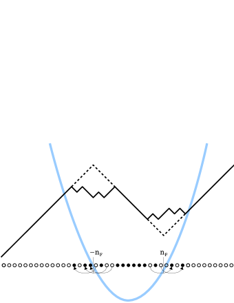
Figure 1: An eigenvalue distribution in the quadratic potential. Black dots stand for the positions of the eigenvalues and white ones are vacant positions. If we draw the right-down and right-up line for the black and white dots, respectively, we obtain the Young diagram drawing above the dots. The $n_{F}$ and $-n_{F}$ mean the positions of two fermi surfaces.

Let us finally discuss the behavior of the eigenvalues $\{n_{i}\}$ for the gaussian model. We first identify the positions of the eigenvalues $n_{i}$ with the so-called Maya diagram. The correspondence between the eigenvalues of the discrete matrix model and a Young diagram is depicted in Fig. 1. We also regard the positions of the eigenvalues as the Fock space of free fermions. The states of the free fermions have two fermi surface. The fermions are exciting from the fermi surfaces and the corresponding Young diagram is scraped away (melting) from the corner. If we determine the constant $c$ by a condition $\sum_{i}n_{i}=\sum_{i}k_{i}$, we have $c=\frac{N+1}{2}$ and the fermi surfaces exist at $\frac{N-1}{2}$ and $-\frac{N-1}{2}$. The ground state distribution is symmetric with respect to the critical point of the quadratic potential, which is now at the origin.

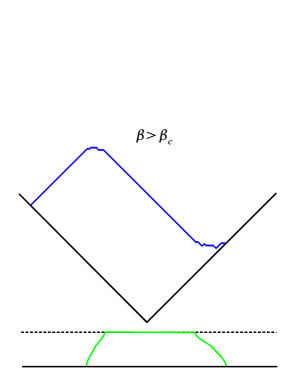
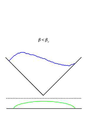
Figure 2: These are results from Monte-Carlo simulations for $N=100$ and $G=0$. When $\beta>\beta_{c}$, the eigenvalues are accumulated around the origin exceeding the maximal value of the density. The corresponding Young diagram has a planar edge. If the inverse temperature is below the critical value $\beta_{c}$, the system enters a different phase. The eigenvalue density behaves as the semi-circle.

This choice or assumption for the ground state is also supported by the numerical analysis of the discrete matrix model (3.13) by using Monte-Carlo simulation. For the symmetric quadratic potential, the ground state is realized in the zero temperature limit where the potential term is dominated and the eigenvalues are symmetrically distributed. We can also see the fermionic eigenvalues are excited from two fermi surface if the repulsive force originated in the Vandermonde determinant is taken into account. We draw some results of the Monte-Carlo simulation for $G=0$ in Fig.2. We vary a combination of the parameters $\beta\equiv g_{s}\mu A$, which can be regarded as the inverse temperature of the system. In the low temperature (large $\beta$) limit, we see that the eigenvalues gather at the origin, namely it approaches to the ground state configuration. The corresponding Young diagram is rigid and has a long planar edge of a rectangle shape. As the temperature becomes higher, the eigenvalues leave from the two fermi surfaces because of the repulsive effect from the Vandermonde determinant. Correspondingly, the Young diagram is crumbling (melting) from the corner. On the other hand, if we define a density of the eigenvalue distribution,

$$\rho(x)=\frac{1}{N}\sum_{i=1}^{N}\delta(x-g_{s}n_{i}),$$ (3.22)

we find that there exists a maximal value of the density reflecting the discreteness of the eigenvalues. A region where the eigenvalue density meets the maximal value corresponds to a planar (right-down) edge of the Young diagram. Looking at the behavior of the eigenvalue distribution (density) or the shape of the Young diagram, we notice a phase transition at a critical temperature. In fact, if the temperature becomes higher, the planar region of the Young diagram finally disappears. From the eigenvalue density point of view, the flat head which hits the maximal value of the density is pinched at the critical temperature and the so-called Wigner’s semi-circle is realized in the high temperature phase. This type of the phase transition is known as the Douglas-Kazakov phase transition of third order [29] by considering a continuum limit of Migdal’s partition function or discrete matrix model. We will discuss it in detail in section 5.

3.2 Nekrasov’s partition function

Here we derive the Nekrasov’s instanton partition function from ${{\rm gYM}_{2}}$ using the similar technique in the previous subsection.

The partition function of the ${{\rm gYM}_{2}}$ is

$$Z=\int{\cal D}A{\cal D}\Phi\exp\left[-\frac{1}{g_{s}}\int_{\Sigma_{G}}{\rm Tr}\,\left(i\Phi F+W(\Phi)\omega\right)\right].$$ (3.23)

To make the eigenvalues of $\Phi$ localize at suitable positions, we choose that critical points of the potential $W(\Phi)$ exist at $x=q_{l}$, namely,

$$W^{\prime}(x)=\mu_{r+1}\prod_{l=1}^{r}(x-q_{l}).$$ (3.24)

The parameters $q_{l}$ will be related with the moduli parameters in four-dimensional $SU(r)$ Yang-Mills theory by a rescaling and we finally allow each $q_{l}$ to have a complex value by an analytic continuation.

The ${{\rm gYM}_{2}}$ (3.23) can be solved exactly by using the previous procedure for Migdal’s partition function. The result is

$$Z=\sum_{\{n_{i}\}}\prod_{1\leq i<j\leq N}\left(g_{s}n_{i}-g_{s}n_{j}\right)^{2-2G}e^{-\frac{A}{g_{s}}\sum_{i}W(g_{s}n_{i})},$$ (3.25)

up to a normalization factor. So the partition function of ${{\rm gYM}_{2}}$ can be regarded as a discretized version of the random matrix model with a generic potential (action). In the case of $\mu_{r+1}\gg 1$, the above summation over $n_{i}$ dominates near the critical points $q_{l}$, so we can assume that $N_{l}$ eigenvalues are around the critical point $q_{l}$ as

$$g_{s}n_{i}=(\underbrace{q_{1}+g_{s}h^{(1)}_{1},\ldots,q_{1}+g_{s}h^{(1)}_{N_{1}}}_{N_{1}},\underbrace{q_{2}+g_{s}h^{(2)}_{1},\ldots,q_{2}+g_{s}h^{(2)}_{N_{2}}}_{N_{2}},\\ \ldots,\underbrace{q_{r}+g_{s}h^{(r)}_{1},\ldots,q_{r}+g_{s}h^{(r)}_{N_{r}}}_{N_{r}}),$$ (3.26)

where $h^{(l)}_{i}$ $(i=1,\ldots,N_{l})$ represent fluctuations around the critical points, which satisfy

$$h^{(l)}_{1}>h^{(l)}_{2}>\cdots>h^{(l)}_{N_{l}},$$ (3.27)

for each $l$. The $U(N)$ gauge symmetry is broken to $\prod_{l=1}^{r}U(N_{l})$ around this configuration. In contrast to the previous Gaussian case (quadratic potential), we can not say the eigenvalues are distributed symmetrically around each critical point in general since we can not ignore effects from neighbor critical points. However, in the large $N$ limit which we will discuss later, the generic potential decouples into a union of the quadratic potentials in an approximation. So we hereafter proceed our analysis by assuming the eigenvalues are symmetrical at each critical point, although this is valid only for a suitable scaling large $N$ limit.

Under this assumption, we introduce a parametrization $\{K_{i}^{(l)}\}$ as

$$h^{(l)}_{i}=K^{(l)}_{i}-i+\frac{N_{l}+1}{2},$$ (3.28)

and we only consider the case $\sum_{i=1}^{N_{l}}g_{s}K_{i}^{(l)}\ll|q_{l}-q_{n}|$ for ${}^{\forall}n\neq l$ so that the lumps of the eigenvalues separate enough each other. Here we have assumed $N_{l}$’s are odd numbers for simplicity. As well as the argument in the previous subsection, $\{K_{i}^{(l)}\}$ is weakly decreasing integer sequence;

$$K^{(l)}_{1}\geq K^{(l)}_{2}\geq\cdots\geq K^{(l)}_{N_{l}},$$ (3.29)

and we call the densest configuration $\{K_{i}^{(l)}=0\}$ as the “ground state” of this system.

Let us next consider excitations from the ground state, that is, non-trivial configurations of $\{K_{i}^{(l)}\}$. Since we assume symmetrical distribution of eigenvalues around each critical point, $\{K_{i}^{(l)}\}$ is assumed to be separated into two parts (positive $K^{(l)}_{i}$ and negative $K^{(l)}_{i}$) as

$$K_{i}^{(l)}=\begin{cases}k_{i}^{(l)}\geq 0,&(i=1,\cdots,\frac{N_{l}-1}{2})\\ -\widetilde{k}_{N_{l}-i+1}^{(l)}\leq 0&(i=\frac{N_{l}+3}{2},\cdots,N_{l}),\end{cases}$$ (3.30)

where both of $\{k_{i}^{(l)}\}$ and $\{\widetilde{k}_{j}^{(l)}\}$ are weakly decreasing sequences of non-negative integer. (We assume $K_{(N_{l}+1)/2}^{(l)}=0$.) If we consider the case that the numbers of the excitations are much smaller than $N_{l}$, most of $\{k_{i}^{(l)}\}$ and $\{\widetilde{k}_{j}^{(l)}\}$ are zero and the non-zero elements express excitations from “fermi surfaces” at $a_{l}\equiv q_{l}+g_{s}\frac{N_{l}-1}{2}$ and $\tilde{a}_{l}\equiv q_{l}-g_{s}\frac{N_{l}-1}{2}$. (See Fig.3.) Note that this decomposition corresponds to the chiral decomposition discussed in [23, 24, 25].

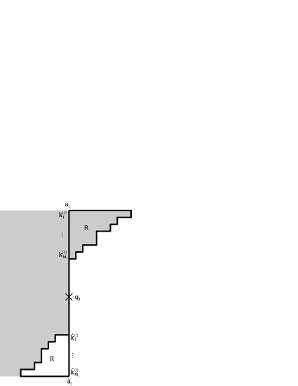
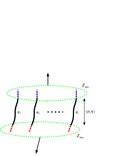
Figure 3: We decompose the excitations from two fermi surfaces. We denote these excitations as $k_{i}^{(l)}$ and $\tilde{k}_{i}^{(l)}$ and positions of the surfaces as $a_{l}$ and $\tilde{a}_{l}$. In the large $N$ limit, the two surfaces are decoupled with each other. And one surface contributes to the instanton partition function.

Using these notations, the potential part of the partition function becomes

$$\frac{A}{g_{s}}\sum_{i=1}^{N}W(g_{s}n_{i}) =\frac{A}{g_{s}}\sum_{l=1}^{r}\sum_{i=1}^{\frac{N_{l}-1}{2}}\left[W\left(a_{l}+g_{s}(k^{(l)}_{i}-i+1)\right)+W\left(a^{-}_{l}-g_{s}(\tilde{k}^{(l)}_{i}-i+1)\right)\right]$$

$$\simeq\frac{A}{g_{s}}\sum_{l=1}^{r}\sum_{i=1}^{\frac{N_{l}-1}{2}}\Bigl{[}W\left(a_{l}+g_{s}(-i+1)\right)+W^{\prime}\left((a_{l}+g_{s}(-i+1)\right)g_{s}k_{i}^{(l)}$$

$$\hskip 79.66771pt+W\left(\widetilde{a}_{l}-g_{s}(-i+1)\right)-W^{\prime}\left((\widetilde{a}_{l}-g_{s}(-i+1)\right)g_{s}\widetilde{k}_{i}^{(l)}\Bigr{]},$$ (3.31)

where we have expanded each term by “small” fluctuations $g_{s}k^{(l)}_{i}$ and $g_{s}\tilde{k}^{(l)}_{i}$. Note that $k_{i}^{(l)}$ and $\widetilde{k}_{i}^{l}$ have non-zero values only for $i\ll N_{l}$, where the arguments of $W^{\prime}$ in (3.31) can be evaluated as

$$a_{l}+g_{s}(-i+1)\simeq\frac{g_{s}N_{l}}{2}+{\cal O}(1).$$ (3.32)

Therefore, from the definition of the potential (3.24), we see that the potential part of the partition function is evaluated as

$$\exp\left[-\frac{A}{g_{s}}\sum_{l=1}^{r}\sum_{i=1}^{N_{l}}W(g_{s}n_{i}^{(l)})\right] \simeq C_{0}\exp\left[-\mu_{r+1}A\sum_{l=1}^{r}\left(\frac{g_{s}N_{l}}{2}\right)^{r}(k_{l}+\widetilde{k}_{l})\right],$$ (3.33)

where $C_{0}$ is the contribution from the ground state; $C_{0}=e^{-\frac{A}{g_{s}}\sum_{l=1}^{r}\sum_{i=1}^{N_{l}}W\left(a_{l}+g_{s}(-i+\frac{N_{l}+1}{2})\right)}$, and we have used a suitable analytic continuation in the anti-chiral sector.

On the other hand, the discrete Vandermonde determinant (measure) part of the partition function is decomposed as

$$\prod_{i\neq j}(g_{s}n_{i}-g_{s}n_{j})=\mu_{++}^{(N)}\mu_{+-}^{(N)}\mu_{-+}^{(N)}\mu_{--}^{(N)}$$ (3.34)

where

$$\mu_{++}^{(N)} = \prod_{(l,i_{l})\neq(n,j_{n})}^{\{N_{l,n}/2\}}\left({a_{l}-a_{n}+g_{s}(k^{(l)}_{i_{l}}-k^{(n)}_{j_{n}}-i_{l}+j_{n})}\right),$$ (3.35)

$$\mu_{+-}^{(N)} = \prod_{(l,i_{l})\neq(n,j_{n})}^{\{N_{l,n}/2\}}\left({a_{l}-\widetilde{a}_{n}+g_{s}(k^{(l)}_{i_{l}}+\tilde{k}^{(n)}_{j_{n}}-i_{l}-j_{n}+1)}\right),$$ (3.36)

$$\mu_{-+}^{(N)} = \prod_{(l,i_{l})\neq(n,j_{n})}^{\{N_{l,n}/2\}}\left({\widetilde{a}_{l}-a_{n}-g_{s}(\tilde{k}^{(l)}_{i_{l}}+k^{(n)}_{j_{n}}-i_{l}-j_{n}+1)}\right),$$ (3.37)

$$\mu_{--}^{(N)} = \prod_{(l,i_{l})\neq(n,j_{n})}^{\{N_{l,n}/2\}}\left({\widetilde{a}_{l}-\widetilde{a}_{n}-g_{s}(\tilde{k}^{(l)}_{i_{l}}-\tilde{k}^{(n)}_{j_{n}}-i_{l}+j_{n})}\right),$$ (3.38)

where the symbol $\{N_{l,n}/2\}$ over the product represents that each $i_{l}$ ($j_{n}$) runs from 1 to $\frac{N_{l}-1}{2}$ ($\frac{N_{n}-1}{2}$), and we have used the suffix $(N)$ to stress that they are defined for finite $N$. Here we find that the cross terms $\mu_{\pm\mp}^{2}$ of are decoupled from the partition function in the large $N$ limit since $a_{l}-a_{n}\sim{\cal O}(1)$, $\widetilde{a}_{l}-\widetilde{a}_{n}\sim{\cal O}(1)$ and $a_{l}-\widetilde{a}_{n}\sim{\cal O}(g_{s}N)$.

Now we would like to take a large $N$ limit. In our case, we must also take the limit of $\mu_{r+1}\to 0$ to recover ${\cal N}{=}2$ SUSY in the four-dimensional space-time, thus it is proper to take the large $N$ limit with $N_{l}=N_{n}$ for all $l=1,\cdots,r$ since the positions of the critical points are in the flat direction of the ${\cal N}{=}2$ SUSY theory. Then, we set $N_{l}$ as

$$N_{l}\equiv 2M+1,\qquad(l=1,\cdots,r)$$ (3.39)

and take the limit $M\to\infty$. In this limit, $\mu_{++}^{(N)}$ can be evaluated as

$$\mu_{++}^{(N)} =Z_{0}(\mbox{\boldmath$a$})\prod_{(l,i_{l})\neq(n,j_{n})}^{M}\left(\frac{a_{l}-a_{n}+g_{s}(k^{(l)}_{i_{l}}-k^{(n)}_{j_{n}}-i_{l}+j_{n})}{a_{l}-a_{n}+g_{s}(-i_{l}+j_{n})}\right)$$

$$\simeq Z_{0}(\mbox{\boldmath$a$})(g_{s}M)^{2rk}\prod_{(l,i)\neq(n,j)}\left(\frac{a_{l}-a_{n}+g_{s}(k^{(l)}_{i}-k^{(n)}_{j}-i+j)}{a_{l}-a_{n}+g_{s}(-i+j)}\right),$$ (3.40)

with

$$Z_{0}(\mbox{\boldmath$a$}) =\prod_{(l,i)\neq(n,j)}\Bigl{(}a_{l}-a_{n}+g_{s}(-i+j)\Bigr{)},$$ (3.41)

where $k=\sum_{l=1}^{r}\sum_{i}k_{i}^{(l)}$ and $i$ and $j$ now run from $1$ to $\infty$. For the proof from the first line to the second line of (3.41), see the appendix A. This normalization factor is coming from a contribution of the ground state to the Vandermonde measure, and will give the perturbative part of the prepotential of the four-dimensional ${\cal N}{=}2$ SUSY gauge theory [43, 1, 44]. In addition, we take a scaling limit $\mu_{r+1}\to 0$ with fixing,

$$(g_{s}M)^{2r}\exp\left(-A\mu_{r+1}(g_{s}M)^{r}\right)\equiv\Lambda^{2r}.$$ (3.42)

On the other hand, we can also show that $\mu_{--}$ gives the same contribution with $\mu_{++}$ under the setup (3.39) since $\widetilde{a}_{l}-\widetilde{a}_{n}$ and $a_{l}-a_{n}$ coincide in the large $N$ limit (3.39). Therefore, in this double scaling limit, the partition function of the ${{\rm gYM}_{2}}$ becomes

$${Z}_{gYM_{2}}=Z_{\rm inst}\left(\mbox{\boldmath$a$};\Lambda\right)^{2}$$ (3.43)

with

$$Z_{\rm inst}\left(\mbox{\boldmath$a$};\Lambda\right) =Z_{0}(\mbox{\boldmath$a$})\sum_{\vec{\mbox{\boldmath$k$}}}\Lambda^{2rk}\prod_{(l,i)\neq(n,j)}\left(\frac{a_{l}-a_{n}+g_{s}(k^{(l)}_{i}-k^{(n)}_{j}+j-i)}{a_{l}-a_{n}+g_{s}(j-i)}\right)^{1-G}.$$ (3.44)

In particular, if we set $G=0$, $Z_{\rm inst}$ coincides with the Nekrasov’s partition function exactly.

Finally we note that, if we introduce the $\theta$-term in the action of the gYM₂, we can easily show that the “QCD scale” $\Lambda$ in (3.42) becomes complex and $\bar{\Lambda}$ appears in $\mu_{--}$. Then, we expect that $\mu_{++}$ and $\mu_{--}$ describe the instanton and the anti-instanton contributions to the prepotential, respectively, and we could verify

$$Z_{gYM_{2}}=\left|Z_{\rm inst}(\mbox{\boldmath$a$};\Lambda)\right|^{2},$$ (3.45)

by taking a suitable analytic continuation of $a$.

4 Adding matters

In this section, we derive the instanton partition function for other ${\cal N}{=}2$ theories from suitable two-dimensional theories. We first consider the ${\cal N}{=}2$ theory with massive hypermultiplets in the adjoint representation, and next we present a formula for quiver gauge theory [28] as a conjecture. We also show that a formula for theory with fundamental hypermultiplets given in [1] is obtained by a flow from the quiver theory.

4.1 Addition of adjoint matter

To construct a two-dimensional theory that provides the instanton counting of the ${\cal N}{=}2$ theory with the massive adjoint hypermultiplet, we first introduce an additional BRST multiplets $(X,\psi_{X})$ and $(Y,\psi_{Y})$ whose (deformed) BRST transformation is given by

$$\begin{array}[]{ll}QX=\psi_{X},&Q\psi_{X}=[\Phi,X]+mX,\\ QY=\psi_{Y},&Q\psi_{Y}=[\Phi,Y]-mY,\end{array}$$ (4.1)

where $X$ and $Y$ are both Hermitian in the adjoint representation of $U(N)$. Using them, we add the following BRST exact expression to the action of the topological field theory (2.5),

$$\delta S_{\rm adj} =\frac{1}{2g_{s}}\int_{\Sigma_{G}}Q\left(Y\psi_{X}-X\psi_{Y}\right)$$

$$=\frac{1}{g_{s}}\int_{\Sigma_{G}}\left(\Phi[X,Y]+mXY-\psi_{X}\psi_{Y}\right),$$ (4.2)

and consider the expectation value in this topological field theory,

$$\left\langle\exp\left[-\frac{1}{g_{s}}\int_{\Sigma_{G}}{\rm Tr}\,\left(i\Phi F+\frac{1}{2}\lambda\wedge\lambda+W(\Phi)\omega\right)\right]\right\rangle_{\rm top},$$ (4.3)

where $W(\Phi)$ is again defined by (3.24). As discussed in the section 2, it can be evaluated as the partition function of a corresponding two-dimensional gauge theory,

$$Z_{\rm adj}=\int{\cal D}A{\cal D}\Phi{\cal D}X{\cal D}Y\exp\left\{-\frac{1}{g_{s}}\int_{\Sigma_{G}}\,{\rm Tr}\,\Bigl{[}i\Phi F+\bigl{(}W(\Phi)+\Phi[X,Y]+mXY\bigr{)}\omega\Bigr{]}\right\},$$ (4.4)

after integrating out $\lambda$, $\psi_{X}$ and $\psi_{Y}$, up to contributions from higher critical points. We assume that these “matter” fields are localized at several points as impurities (sources) on the Riemann surface $\Sigma_{G}$ as well as the Hitchin system in [45].

In the following, we show that (4.4) reproduces the instanton counting of the four-dimensional ${\cal N}{=}2$ theory with the massive hypermultiplet in the adjoint representation given in [27, 1]. Fixing the gauge by $\Phi_{\alpha}=0$, as discussed in the section 3.1, we obtain (3.25) by performing the Gaussian integrals over the gauge fields $A_{\alpha}$ and the ghost fields $(c_{\alpha},\bar{c}_{\alpha})$. In the case of (4.4), we must also perform the integration over $X$ and $Y$,

$$\int\prod_{i\neq j}^{N}{\cal D}X_{ij}{\cal D}Y_{ij}\exp\left\{-\frac{A}{g_{s}}\sum_{i\neq j}^{N}\left(m+\lambda_{i}-\lambda_{j}\right)X_{ij}Y_{ij}\right\}=\prod_{i\neq j}^{N}\frac{1}{m+\lambda_{i}-\lambda_{j}},$$ (4.5)

where we use the assumption that $X$ and $Y$ are delta-functionally localized at a point on $\Sigma_{G}$. Then, except for an overall factor, (4.4) can be evaluated as

$$Z_{\rm adj}=\sum_{n_{i}\in\mathbb{Z}}\prod_{i\neq j}^{N}\frac{\left(g_{s}n_{i}-g_{s}n_{j}\right)^{1-G}}{m+g_{s}n_{i}-g_{s}n_{j}}e^{-\frac{A}{g_{s}}\sum_{i=1}^{N}W(g_{s}n_{i})}.$$ (4.6)

Now we take the double scaling limit $N\to\infty$ and $\mu_{r+1}\to 0$ with the condition (3.42). Repeating the discussion in the section 3.2, we can show that the partition function (4.4) becomes

$$Z_{\rm adj}=Z_{\rm inst}^{\rm adj}\left(\mbox{\boldmath$a$},m;\Lambda\right)^{2}$$ (4.7)

with

$$Z_{\rm inst}^{\rm adj} =Z_{\rm pert}^{\rm adj}(\mbox{\boldmath$a$},m)\sum_{\vec{\mbox{\boldmath$k$}}}\Lambda^{2rk}\prod_{(l,i)\neq(n,j)}\left(\frac{a_{l}-a_{n}+g_{s}(k^{(l)}_{i}-k^{(n)}_{j}+j-i)}{a_{l}-a_{n}+g_{s}(j-i)}\right)^{1-G}$$

$$\hskip 99.58464pt\times\frac{m+a_{l}-a_{n}+g_{s}(j-i)}{m+a_{l}-a_{n}+g_{s}(k^{(l)}_{i}-k^{(n)}_{j}+j-i)},$$ (4.8)

where

$$Z_{\rm pert}^{\rm adj}(\mbox{\boldmath$a$},m) =\prod_{(l,i)\neq(n,j)}\frac{\left(a_{l}-a_{n}+g_{s}(j-i)\right)^{1-G}}{m+a_{l}-a_{n}+g_{s}(j-i)}.$$ (4.9)

If we set $G=0$, the chiral part $Z_{\rm inst}^{\rm adj}$ reproduces the instanton counting for the ${\cal N}{=}2$ theory with the massive adjoint hypermultiplet. Here we have again used the fact that $\widetilde{a}_{l}-\widetilde{a}_{n}$ can be replaced with $a_{l}-a_{n}$ under the condition (3.39).

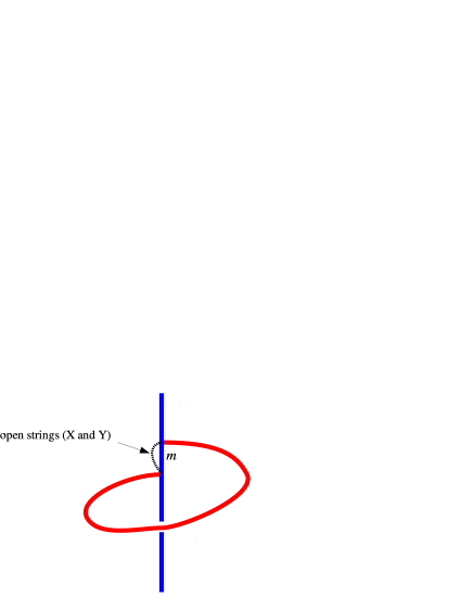
	$\begin{array}[]{c}\Longrightarrow\\ m\rightarrow 0\end{array}$
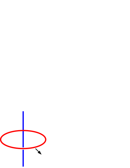
(a)		(b)

Figure 4: A brane configuration of ${\cal N}{=}2$ theory with adjoint hypermultiplets. D4-branes are wrapping around a circle with a shift of the end points on a NS5-brane. The shift disappears in the massless limit and the D4-branes can be removed from the NS5-brane. T-duals of these brane configurations explain why the effective genus in the instanton partition function is increased by one.

We would like to comment on the massless limit of the above model. If we see the expressions (4.8) and (4.9), we notice that the contribution from $X$ and $Y$ cancels one of the $(1-G)$ contributions from ${{\rm gYM}_{2}}$ in the limit of $m\to 0$. This means that the genus $G$ of the Riemann surface effectively shifts to $G+1$. This phenomenon can be easily understood by using a brane configuration for the $G=0$ case. The brane configuration for ${\cal N}{=}2^{*}$ (Donagi-Witten) [46] is shown in Fig.4 where $N$ D4-branes are ending on a single NS5-brane and wrapping around a compact circle. The end points of the D4-branes are separated by $m$. Open strings between two end points have a minimal length and get mass proportional to $m$. They correspond to the hypermultiplets $X$ and $Y$. In the massless limit, the theory enhances to ${\cal N}{=}4$ since the two adjoint hypermultiplets are put into the ${\cal N}{=}4$ vector multiplet. This means the D4-branes can be removed from the NS5-brane in the brane configuration and they are T-dual to parallel D3-branes. T-dual of the brane configuration maps the D4-branes to the D5-branes wrapping on $S^{2}$ and the NS5-brane to a deficit in the geometry. On the other hand, the D4-branes wrapping the compact circle without any shift is the T-dual of D5-branes wrapping on $T^{2}$ where the SUSY enhances to ${\cal N}{=}4$. Therefore, we expect that two punctures on $S^{2}$ corresponding to the end points on the NS5-brane join with each other and the topology changes from $S^{2}$ to $T^{2}$ in the massless limit, namely, the genus of the cycle is increased by one. This phenomenon should be extended to any genus $G$. If two punctures on the Riemann surface with genus $G$ join in the massless limit, the genus is increased by one. This picture agrees with our derived formula.

4.2 Quiver theory

In this succeeding subsection, we construct a two-dimensional theory which is thought to provide the instanton counting of the ${\cal N}{=}2$ $A_{2}$-type quiver gauge theory. The generalization to an arbitrary $A_{n}$-type quiver theory should be straightforward.

The $A_{2}$ quiver theory is realized on two Riemann surfaces which intersect at a point. Bi-fundamental matters in the quiver gauge theory come from open strings connecting D-branes wrapping on the Riemann surfaces independently. So let us consider the system with $N_{1}$ D-strings on Riemann surface $\Sigma_{G_{1}}$ with genus $G_{1}$ and $N_{2}$ D-strings on $\Sigma_{G_{2}}$ with genus $G_{2}$. As discussed in the section 2, the low energy effective theory of this system is a topologically twisted theory constructed from BRST multiplets $(A_{1},\lambda_{1},\Phi_{1})$ and $(A_{2},\lambda_{2},\Phi_{2})$, $(\bar{\Phi}_{1},\eta_{1})$ and $(\bar{\Phi}_{2},\eta_{2})$, and $(H_{1},\chi_{1})$ and $(H_{2},\chi_{2})$, which are in the adjoint representation of $U(N_{1})$ and $U(N_{2})$, respectively. The BRST transformations are given as well as (2.3) and (2.4), and the action is given by

$$S_{\rm top}=Q\Bigl{(} \frac{1}{h_{1}^{2}}\int_{\Sigma_{G_{1}}}{\rm Tr}\,_{N_{1}}\Xi(A_{1},\lambda_{1},\Phi_{1},\bar{\Phi}_{1},\eta_{1},H_{1},\chi_{1})$$

$$+\frac{1}{h_{2}^{2}}\int_{\Sigma_{G_{2}}}{\rm Tr}\,_{N_{2}}\Xi(A_{2},\lambda_{2},\Phi_{2},\bar{\Phi}_{2},\eta_{2},H_{2},\chi_{2})\Bigr{)}.$$ (4.10)

where ${\rm Tr}\,_{N_{a}}$ denotes the trace over an $N_{a}\times N_{a}$ matrix, and the function $\Xi$ is defined like (2.6). This theory is again independent of the coupling constants $h_{1}$ and $h_{2}$.

As in section 2, we first consider following observables of the topological field theory,

$$e^{-\frac{1}{g_{s}}I_{2}^{(a)}}\equiv\exp\left\{-\frac{1}{g_{s}}\int_{\Sigma_{G_{a}}}{\rm Tr}\,_{N_{a}}\left(i\Phi_{a}F_{a}+\frac{1}{2}\lambda_{a}\wedge\lambda_{a}+W_{a}(\Phi_{a})\omega_{a}\right)\right\},\qquad(a=1,2)$$ (4.11)

where $\omega_{a}$ is the volume form on $\Sigma_{G_{a}}$ and we assume that the potentials $W_{1}(x)$ and $W_{2}(x)$ satisfy

$$W^{\prime}_{1}(x) =\mu_{r+1}(x-q^{(1)}_{1})\cdots(x-q^{(1)}_{r}),$$ (4.12)

$$W^{\prime}_{2}(x) =\nu_{s+1}(x-q^{(2)}_{1})\cdots(x-q^{(2)}_{s}),$$ (4.13)

respectively. If we evaluate the expectation value of $e^{-\frac{1}{g_{s}}I_{2}}$ in the topological field theory, we obtain the product of Nekrasov’s partition functions corresponding to pure ${\cal N}{=}2$ SYM theories with the gauge groups $SU(r)\times SU(s)$ after taking a suitable large $N$ limit.

Furthermore, we would like to construct another “potential term” that produces the quiver-type interaction in the four-dimensional ${\cal N}{=}2$ theory. To achieve this, we again introduce an additional BRST multiplets $(B,\psi_{B})$ and $({\widetilde{B}},\psi_{\widetilde{B}})$ which are $N_{1}\times N_{2}$ and $N_{2}\times N_{1}$ matrices, respectively. The BRST transformations are given by

$$QB =\psi_{B},\quad Q\psi_{B}=\Phi_{1}B-B\Phi_{2},$$ (4.14)

$$Q{\widetilde{B}} =-\psi_{\widetilde{B}},\quad Q\psi_{\widetilde{B}}={\widetilde{B}}\Phi_{1}-\Phi_{2}{\widetilde{B}},$$ (4.15)

or, in component,

$$(QB)_{i_{1}i_{2}} =(\psi_{B})_{i_{1}i_{2}},\quad(Q{\psi_{B}})_{i_{1}i_{2}}=\sum_{j_{1}=1}^{N_{1}}(\Phi_{1})_{i_{1}j_{1}}B_{j_{1}i_{2}}-\sum_{j_{2}=1}^{N_{2}}B_{i_{1}j_{2}}(\Phi_{2})_{j_{2}i_{2}},$$ (4.16)

$$(Q{\widetilde{B}})_{i_{2}i_{1}} =-(\psi_{\widetilde{B}})_{i_{2}i_{1}},\quad(Q{\psi_{\widetilde{B}}})_{i_{2}i_{1}}=\sum_{j_{1}=1}^{N_{1}}{\widetilde{B}}_{i_{2}j_{1}}(\Phi_{1})_{j_{1}i_{1}}-\sum_{j_{2}=1}^{N_{2}}(\Phi_{2})_{i_{2}j_{2}}{\widetilde{B}}_{j_{2}i_{1}},$$ (4.17)

where $i_{1},j_{1}=1,\cdots,N_{1}$ and $i_{2},j_{2}=1,\cdots,N_{2}$. We assume that these “matter” fields are also localized at points as impurities. Now let us define the topological field theory by adding the following BRST exact term,

$$\delta S_{\rm quiv} \equiv\frac{1}{2g_{s}}\int_{\Sigma_{G_{1}}\cup\Sigma_{G_{2}}}Q{\rm Tr}\,\left({\widetilde{B}}\psi_{B}+B\psi_{\widetilde{B}}\right)$$

$$=\frac{1}{g_{s}}\int_{\Sigma_{G_{1}}\cup\Sigma_{G_{2}}}\left[{\rm Tr}\,_{N_{2}}\left({\widetilde{B}}\Phi_{1}B\right)-{\rm Tr}\,_{N_{1}}\left(B\Phi_{2}{\widetilde{B}}\right)-{\rm Tr}\,_{N_{2}}\left(\psi_{\widetilde{B}}\psi_{B}\right)\right],$$ (4.18)

to the action (4.10). The instanton partition function of the quiver gauge theory can be obtained from the evaluation of the expectation value,

$$\left\langle e^{-\frac{1}{g_{s}}\left(I_{2}^{(1)}+I_{2}^{(2)}\right)}\right\rangle_{\rm top}.$$ (4.19)

If we ignore contributions from higher critical points again, it reduces to the partition function of a two-dimensional theory,

$$Z_{\rm quiv}=\int {\cal D}A_{1}{\cal D}\Phi_{1}{\cal D}A_{2}{\cal D}\Phi_{2}{\cal D}B{\cal D}{\widetilde{B}}$$

$$\exp\Biggl{\{}-\frac{1}{g_{s}}\int_{\Sigma_{G_{1}}}\left[{\rm Tr}\,_{N_{1}}\left(i\Phi_{1}F_{1}+W_{1}(\Phi_{1})\omega_{1}\right)+{\rm Tr}\,_{N_{2}}\left({\widetilde{B}}\Phi_{1}B\right)\omega_{1}\right]$$

$$\hskip 28.45274pt-\frac{1}{g_{s}}\int_{\Sigma_{G_{2}}}\left[{\rm Tr}\,_{N_{2}}\left(i\Phi_{2}F_{2}+W_{2}(\Phi_{2})\omega_{2}\right)-{\rm Tr}\,_{N_{1}}\left(B\Phi_{2}{\widetilde{B}}\right)\omega_{2}\right]\Biggr{\}},$$ (4.20)

where we have used the assumption that $\Phi_{1}$ $(\Phi_{2})$ takes non-zero value only on $\Sigma_{1}$ $(\Sigma_{2})$. Repeating the discussion in the section 3.2, the partition function (4.20) can be expressed as a summation over sets of integers $\{n^{(1)}_{i_{1}}\}$ and $\{n^{(2)}_{i_{2}}\}$;

$$Z_{\rm quiv}=\sum_{n^{(1)}_{i_{1}},n^{(2)}_{i_{2}}\in\mathbb{Z}} \prod_{i_{1}\neq j_{1}}^{N_{1}}\left(g_{s}n_{i_{1}}^{(1)}-g_{s}n_{j_{1}}^{(1)}\right)^{1-G_{1}}\prod_{i_{2}\neq j_{2}}^{N_{2}}\left(g_{s}n_{i_{2}}^{(2)}-g_{s}n_{j_{2}}^{(2)}\right)^{1-G_{2}}$$

$$\times\prod_{i_{1}=1}^{N_{1}}\prod_{i_{2}=1}^{N_{2}}\left(g_{s}n_{i_{1}}^{(1)}-g_{s}n_{i_{2}}^{(2)}\right)^{-1}e^{-\frac{A_{1}}{g_{s}}\sum_{i_{1}=1}^{N_{1}}W_{1}(g_{s}n_{i_{1}}^{(1)})}e^{-\frac{A_{2}}{g_{s}}\sum_{i_{2}=1}^{N_{2}}W_{2}(g_{s}n_{i_{2}}^{(2)})},$$ (4.21)

where $A_{1}$ and $A_{2}$ are the areas of $\Sigma_{G_{1}}$ and $\Sigma_{G_{2}}$, respectively. In deriving (4.21), we have used the assumption that $B$’s are localized at points.

Now let us evaluate (4.21) in the limit of $N_{1}\to\infty$, $N_{2}\to\infty$ and $\mu_{r+1}\to 0$ and $\nu_{s+1}\to 0$ with a suitable scaling. Since it is almost the product of the partition function of gYM₂ on $\Sigma_{G_{1}}$ and that on $\Sigma_{G_{2}}$, we can apply the same discussion to derive (3.43). Namely, we can assume that there are $2N^{(1)}_{l_{1}}+1$ eigenvalues around $q_{l_{1}}^{(1)}$ and $2N^{(2)}_{l_{2}}+1$ eigenvalues around $q_{l_{2}}^{(2)}$, respectively, whose distribution can be expressed as excitations from the ground states, i.e. the densest and symmetrical distribution of eigenvalues around the critical points. When $N_{1}$ and $N_{2}$ are sufficiently large, the excitations are thought to occur at the “fermi levels” at $a^{(a)}_{l_{a}}=q^{(a)}_{l_{a}}+g_{s}\frac{N_{l_{a}}-1}{2}$ and $\widetilde{a}^{(a)}_{l_{a}}=q^{(a)}_{l_{a}}-g_{s}\frac{N_{l_{a}}-1}{2}$ $(a=1,2)$, which are labeled by sets of partitions $(\{k_{i_{1}}^{l_{1}}\}_{l_{1}=1}^{r},\{k_{i_{2}}^{l_{2}}\}_{l_{2}=1}^{s})$ and $(\{\widetilde{k}_{i_{1}}^{l_{1}}\}_{l_{1}=1}^{r},\{\widetilde{k}_{i_{2}}^{l_{2}}\}_{l_{2}=1}^{s})$. In the case of $\mu_{r+1}\to 0$ and $\nu_{s+1}\to 0$, it is natural to assume $N^{(a)}_{l_{a}}=2M_{a}+1$ for each $l_{a}$, and we can take the double scaling limit $M_{1}\to\infty$, $M_{2}\to\infty$ and $\mu_{r+1}\to 0$ and $\nu_{s+1}\to 0$ with fixing,

$$(g_{s}M_{1})^{2r}\exp\left(-A_{1}\mu_{r+1}(g_{s}M_{1})^{r}\right) \equiv\Lambda_{1}^{2r},$$

$$(g_{s}M_{2})^{2s}\exp\left(-A_{2}\mu_{s+1}(g_{s}M_{2})^{r}\right) \equiv\Lambda_{2}^{2s}.$$ (4.22)

(See the discussion around (3.42).) In this limit, the partition function (4.21) becomes

$$Z_{\rm quiv}=\left[Z_{\rm inst}\left(\mbox{\boldmath$a$}^{(1)};\Lambda_{1}\right)Z_{\rm inst}\left(\mbox{\boldmath$a$}^{(2)};\Lambda_{2}\right)Z_{12}\left(\mbox{\boldmath$a$}^{(1)},\mbox{\boldmath$a$}^{(2)};M_{1}-M_{2}\right)\right]^{2},$$ (4.23)

where $Z_{\rm inst}\left(\mbox{\boldmath$a$};\Lambda\right)$ is given in (3.43) and

$$Z_{12} \left(\mbox{\boldmath$a$}^{(1)},\mbox{\boldmath$a$}^{(2)};M_{1}-M_{2}\right)$$

$$=\sum_{\vec{\mbox{\boldmath$k$}}^{(1)},\vec{\mbox{\boldmath$k$}}^{(2)}}\prod_{(l_{1},i_{1})}\prod_{(l_{2},i_{2})}\left(a_{l_{1}}^{(1)}-a_{l_{2}}^{(2)}+g_{s}(M_{1}-M_{2})+g_{s}\left(k_{i_{1}}^{(l_{1})}-k_{i_{2}}^{(l_{2})}-i_{1}+i_{2}\right)\right)^{-1}.$$ (4.24)

Here we have ignored terms that contain $g_{s}(M_{1}+M_{2})$ since it suppresses the fluctuations by $\vec{\mbox{\boldmath$k$}}_{1}$ and $\vec{\mbox{\boldmath$k$}}_{2}$. Therefore, the partition function (4.20) is factorized into two parts in the double scaling limit. Especially, under the additional condition $M_{1}=M_{2}$, it can be expressed as

$$Z_{\rm quiv}=Z_{\rm inst}^{\rm quiv}\left(\mbox{\boldmath$a$}^{(1)},\mbox{\boldmath$a$}^{(2)};\Lambda_{1},\Lambda_{2};G_{1},G_{2}\right)^{2},$$ (4.25)

with

$$Z_{\rm inst}^{\rm quiv} \left(\mbox{\boldmath$a$}^{(1)},\mbox{\boldmath$a$}^{(2)};\Lambda_{1},\Lambda_{2};G_{1},G_{2}\right)=Z_{\rm pert}^{\rm quiv}\left(\mbox{\boldmath$a$}^{(1)},\mbox{\boldmath$a$}^{(2)}\right)\sum_{\vec{\mbox{\boldmath$k$}}^{(1)},\vec{\mbox{\boldmath$k$}}^{(2)}}\Lambda_{1}^{k_{1}}\Lambda_{2}^{k_{2}}$$

$$\times\prod_{(l_{1},i_{1})\neq(n_{1},j_{1})}\left(\frac{a^{(1)}_{l_{1}}-a^{(1)}_{n_{1}}+g_{s}(k^{(l_{1})}_{i_{1}}-k^{(n_{1})}_{j_{1}}+j_{1}-i_{1})}{a^{(1)}_{l}-a^{(1)}_{n}+g_{s}(j_{1}-i_{1})}\right)^{1-G_{1}}$$

$$\times\prod_{(l_{2}.i_{2})\neq(n_{2},j_{2})}\left(\frac{a^{(2)}_{l_{2}}-a^{(2)}_{n_{2}}+g_{s}(k^{(l_{2})}_{i_{2}}-k^{(n_{2})}_{j_{2}}+j_{2}-i_{2})}{a^{(2)}_{l}-a^{(2)}_{n}+g_{s}(j_{2}-i_{2})}\right)^{1-G_{2}}$$

$$\times\prod_{(l_{1},i_{1})}\prod_{(l_{2},i_{2})}\frac{a_{l_{1}}^{(1)}-a_{l_{2}}^{(2)}+g_{s}\left(-i_{1}+i_{2}\right)}{a_{l_{1}}^{(1)}-a_{l_{2}}^{(2)}+g_{s}\left(k_{i_{1}}^{(l_{1})}-k_{i_{2}}^{(l_{2})}-i_{1}+i_{2}\right)},$$ (4.26)

and

$$Z_{\rm pert}^{\rm quiv} \left(\mbox{\boldmath$a$}^{(1)},\mbox{\boldmath$a$}^{(2)}\right)$$

$$=\prod_{(l_{1},i_{1})\neq(n_{1},j_{1})}\left(a_{l_{1}}^{(1)}-a_{n_{1}}^{(1)}+g_{s}(j_{1}-i_{1})\right)^{1-G_{1}}\prod_{(l_{2},i_{2})\neq(n_{2},j_{2})}\left(a_{l_{2}}^{(2)}-a_{n_{2}}^{(2)}+g_{s}(j_{2}-i_{2})\right)^{1-G_{2}}$$

$$\hskip 28.45274pt\times\prod_{(l_{1},i_{1})}\prod_{(l_{2},i_{2})}\left(a_{l_{1}}^{(1)}-a_{l_{2}}^{(2)}+g_{s}\left(-i_{1}+i_{2}\right)\right)^{-1},$$ (4.27)

where $k_{a}=\sum_{l_{a},i_{a}}k_{i_{a}}^{(l_{a})}$. We have again used the fact that $\widetilde{a}_{l_{a}}^{(a)}$ can be replaced by $a_{l_{a}}^{(a)}$ as long as $M_{1}=M_{2}$. We conjecture that the expression (4.26) gives the instanton contribution to the ${\cal N}{=}2$ $A_{2}$-quiver theory with the gauge symmetry $SU(r)\times SU(s)$ with the bi-fundamental matters.

4.3 Fundamental matters

In this subsection, we derive the instanton partition function for ${\cal N}{=}2$ theories with the hypermultiplets in the fundamental representation from a two-dimensional gauge theory. Since we already have the formula for the quiver theory in hand, it can be obtained by considering a limited case of the previous section, namely, the limit of $A_{2}\to\infty$.

Let us start with the partition function (4.21). Before taking the double scaling limit (4.22), we perform the limit of $A_{2}\to\infty$. Then the eigenvalues $\{n_{i_{2}}^{(2)}\}$ cannot excite from the ground state since the potential becomes infinitely deep effectively, that is, we must take

$$k_{i_{2}}^{l_{2}}=0,\quad\widetilde{k}_{i_{2}}^{l_{2}}=0,$$ (4.28)

for all $l_{2}$ and $i_{l_{2}}$. Putting $\Lambda_{1}$ to $\Lambda$, $G_{1}$ to $G$, $\{a_{l_{1}}^{(1)}\}_{l_{1}=1}^{r}$ to $\{a_{l}\}_{l=1}^{r}$ and $\{a_{l_{2}}^{(2)}\}_{l_{2}=1}^{s}$ to $\{m_{f}\}_{f=1}^{s}$, the factorized partition function (4.26) becomes

$$Z_{\rm quiv}\Bigr{|}_{A_{2}\to\infty}=Z_{\rm inst}^{\rm fund}\left(\mbox{\boldmath$a$},\mbox{\boldmath$m$};\Lambda;G\right)^{2}$$ (4.29)

with

$$Z_{\rm inst}^{\rm fund}\left(\mbox{\boldmath$a$},\mbox{\boldmath$m$};\Lambda;G\right)=Z_{\rm pert}^{\rm fund}\left(\mbox{\boldmath$a$},\mbox{\boldmath$m$}\right)\sum_{\vec{\mbox{\boldmath$k$}}}\Lambda^{k} \prod_{(l,i)\neq(n,j)}\left(\frac{a_{l}-a_{n}+g_{s}(k^{(l)}_{i}-k^{(n)}_{j}+j-i)}{a_{l}-a_{n}+g_{s}(j-i)}\right)^{1-G}$$

$$\times\prod_{(l,i)}\prod_{(f,j)}\frac{a_{l}-m_{f}+g_{s}\left(-i+j\right)}{a_{l}-m_{f}+g_{s}\left(k_{i}^{(l)}-i+j\right)},$$ (4.30)

where

$$Z_{\rm pert}^{\rm fund}\left(\mbox{\boldmath$a$},\mbox{\boldmath$m$}\right) =\prod_{(l,i)\neq(n,j)}\left(a_{l}-a_{n}+g_{s}(j-i)\right)^{1-G}\prod_{(l,i)}\prod_{(f,j)}\left(a_{l}-m_{f}+g_{s}\left(-i+j\right)\right)^{-1}.$$ (4.31)

If we set $G=0$, (4.30) is nothing but the instanton counting for ${\cal N}{=}2$ theory with massive fundamental hypermultiplets given in [1]. This fact supports our conjecture presented in the previous subsection.

5 Continuum Limit

5.1 Eigenvalue density vs profile function

We first would like to mention on the relationship between the eigenvalue density and the profile function introduced in [1]. Both quantities are essentially connected through difference equations. The profile function expression of the discrete matrix model is useful to see a series expansion with respect to $g_{s}$, which gives the graviphoton corrections to ${\cal N}{=}2$ SUSY gauge theory.

We now define an eigenvalue density for (3.25) in the standard way,

$$\rho(x)\equiv\frac{1}{N}\sum_{i=1}^{N}\delta(x-g_{s}n_{i}),$$ (5.1)

which follows $\int dx\rho(x)=1$. The Vandermonde determinant part can be written in terms of the eigenvalue density as

$$\prod_{1\leq i<j\leq N}(g_{s}n_{i}-g_{s}n_{j})^{2-2G}=\exp\left\{(1-G)N^{2}-\int dxdy\log(x-y)\rho(x)\rho(y)\right\},$$ (5.2)

where the integral stands for a principal part. Similarly, the potential part is

$${\rm Tr}\,W(\Phi)=N\int dxW(x)\rho(x).$$ (5.3)

Thus we can write the partition function of the discrete matrix model (3.25) as

$$Z=\sum_{\{\rho(x)\}}\exp\Big{\{}(1-G)N^{2}-\int dxdy\log(x-y)\rho(x)\rho(y)-\frac{AN}{g_{s}}\int dxW(x)\rho(x)\Big{\}},$$ (5.4)

where $\{\rho(x)\}$ denotes the possible sets of the eigenvalue density $\rho(x)$.

Here we introduce a function $\gamma_{g_{s}}(x)$ which obeys the following difference equation with respect to the finite parameter $g_{s}$;

$$\gamma_{g_{s}}(x+g_{s})+\gamma_{g_{s}}(x-g_{s})-2\gamma_{g_{s}}(x)=\log x.$$ (5.5)

Then the integral in (5.2) can be rewritten as

$$-\int dxdy \log(x-y)\rho(x)\rho(y)$$

$$=-\int dxdy\Bigl{(}\gamma_{g_{s}}(x-y+g_{s})+\gamma_{g_{s}}(x-y-g_{s})-2\gamma_{g_{s}}(x-y)\Bigr{)}\rho(x)\rho(y)$$

$$=--\int dxdy\,\gamma_{g_{s}}(x-y){\mit\Delta}\rho(x){\mit\Delta}\rho(y),$$ (5.6)

where

$${\mit\Delta}\rho(x)\equiv\rho(x+\frac{g_{s}}{2})-\rho(x-\frac{g_{s}}{2}),$$ (5.7)

and we have used the fact that the integral measure is invariant under a constant shift $x\rightarrow x\pm g_{s}/2$. Similarly, the potential term can be expressed as

$${\rm Tr}\,W(\Phi)=-N\int dx\,U(x){\mit\Delta}\rho(x),$$ (5.8)

using the function $U(x)$ satisfying the relation,

$$U(x+\frac{g_{s}}{2})-U(x-\frac{g_{s}}{2})=W(x).$$ (5.9)

For $r$-th order polynomial potential, we generally have the $(r+1)$-th order polynomial $U(x)$. For example, for the quadratic potential $W(x)=\frac{\mu}{2}x^{2}$, $U(x)$ is given by

$$U(x)=\frac{\mu}{2}\left(\frac{1}{3g_{s}}x^{3}-\frac{g_{s}}{12}x\right),$$ (5.10)

up to an integral constant. Then the partition function (5.4) is expressed as

$$Z=\sum_{\{\rho(x)\}}\exp\Bigl{\{} -(1-G)N^{2}-\int dxdy\,\gamma_{g_{s}}(x-y){\mit\Delta}\rho(x){\mit\Delta}\rho(y)+\frac{AN}{g_{s}}\int dxU(x){\mit\Delta}\rho(x)\Bigr{\}},$$ (5.11)

using the expression ${\mit\Delta}\rho(x)$.

By the way, there is another useful instrument to describe the discrete matrix model; the profile function of the Young diagram utilized in [1],

$$f_{\mbox{\boldmath$k$}}(x;g_{s}) \equiv|x|+\sum_{i=1}^{\infty}\Bigl{[}|x-g_{s}(k_{i}-i+1)|-|x-g_{s}(k_{i}-i)|+|x+g_{s}i|-|x+g_{s}(i-1)|\Bigr{]}$$

$$=\sum_{i=1}^{\infty}\Bigl{[}\left|x-g_{s}(k_{i}-i+1)\right|-\left|x-g_{s}(k_{i}-i)\right|\Bigr{]},$$ (5.12)

where $\{k_{i}\}$ is a sequence of non-increasing non-negative integers. We assume that $k_{i}=0$ for $i>N$. This function is closely related to ${\mit\Delta}\rho(x)$ introduced above. To see it, let us consider the case where the discrete eigenvalues $\{n_{i}\}$ are decomposed into $r$ decoupled lumps starting from $a_{l}$ $(l=1,\cdots,r)$. The corresponding eigenvalue density is

$$\rho(x)=\frac{1}{N}\sum_{l=1}^{r}\sum_{i_{l}=1}^{N_{l}}\delta\left(x-a_{l}-g_{s}\left(k_{i_{l}}^{(l)}-i+\frac{1}{2}\right)\right),$$ (5.13)

where $N=N_{1}+\cdots+N_{r}$, $\{k_{i_{l}}^{(l)}\}_{i_{l}=1}^{N_{l}}$ is a sequence of non-increasing non-negative integer, and $1/2$ in the delta function is a convention. Particularly, if we define the eigenvalue density for the “ground state” by setting all $k^{(l)}_{i}$ to be zero,

$$\rho_{0}(x)=\frac{1}{N}\sum_{l=1}^{r}\sum_{i_{l}=1}^{N_{l}}\delta\left(x-a_{l}+g_{s}\left(i_{l}-\frac{1}{2}\right)\right),$$ (5.14)

we find

$${\mit\Delta}\rho_{0}(x) \equiv\rho_{0}(x+\frac{g_{s}}{2})-\rho_{0}(x-\frac{g_{s}}{2})$$

$$=\frac{1}{N}\sum_{l=1}^{r}\Bigl{(}\delta(x-a_{l}+g_{s}N_{l})-\delta(x-a_{l})\Bigr{)},$$ (5.15)

since the intermediate $\delta$-functions are canceled with each other. Using (5.13), we can easily show that ${\mit\Delta}\rho(x)$ and the (colored) profile function is related by

$$-\frac{1}{2N}\sum_{l=1}^{r}f^{\prime\prime}_{\mbox{\boldmath$k$}^{(l)}}(x-a_{l}) ={\mit\Delta}\rho(x)-\frac{1}{N}\sum_{l=1}^{r}\delta(x-a_{l}+g_{s}N_{l}),$$ (5.16)

where the second term in r.h.s. is a counterpart of the contribution to the summation from $N_{l}$ to infinity.

Now we have a dictionary to translate the eigenvalue density into the profile function in hand. As an application, let us write down the normalized Vandermonde determinant (measure part),

$$\mu_{\vec{\mbox{\boldmath$k$}}}^{2}(\mbox{\boldmath$a$},g_{s})\equiv\prod_{(l,i_{l})\neq(n,j_{n})}\left(\frac{a_{l}-a_{n}+g_{s}(k^{(l)}_{i_{l}}-k^{(n)}_{j_{n}}+j_{n}-i_{l})}{a_{l}-a_{n}+g_{s}(j_{n}-i_{l})}\right),$$ (5.17)

using both of the eigenvalue density and the profile function. In terms of the eigenvalue density, (5.17) can be written as

$$\mu_{\vec{\mbox{\boldmath$k$}}}^{2}(\mbox{\boldmath$a$},g_{s})=\exp\left\{-N^{2}-\int dxdy\,\gamma_{g_{s}}(x-y)({\mit\Delta}\rho(x){\mit\Delta}\rho(y)-{\mit\Delta}\rho_{0}(x){\mit\Delta}\rho_{0}(y))\right\}.$$ (5.18)

On the other hand, it can be also written as

$$\mu_{\vec{\mbox{\boldmath$k$}}}^{2}(\mbox{\boldmath$a$},g_{s})=\exp\Bigg{\{} -\frac{1}{4}-\int dxdy\gamma_{g_{s}}(x-y)\sum_{l\neq n}f^{\prime\prime}_{\mbox{\boldmath$k$}^{(l)}}(x-a_{l})f^{\prime\prime}_{\mbox{\boldmath$k$}^{(n)}}(x-a_{n})$$

$$+\int dx\sum_{l,n}\gamma_{g_{s}}(x-a_{l}+g_{s}N_{l})\left(f^{\prime\prime}_{\mbox{\boldmath$k$}^{(n)}}(x-a_{n})-2\delta(x-a_{n})\right)$$

$$+\sum_{l\neq n}\gamma_{g_{s}}(a_{l}-a_{n})\Bigg{\}},$$ (5.19)

using the profile function. The second term in the exponential represents the finite $N$ effect (cut-off at $g_{s}N_{l}$) and the third is the perturbative contribution to the prepotential. These results also agree with [5] up to irrelevant constants.

5.2 Dijkgraaf-Vafa theory and Douglas-Kazakov phase transition

The discrete version of the matrix model (3.25) has obviously a continuous limit of $g_{s}\rightarrow 0$. In this limit, the summation over a set of possible integers reduces to an integration over continuous variables if we restrict the case as $G=0$ (on sphere),

$$Z=\int\prod_{i=1}^{N}d\lambda_{i}\prod_{i<j}(\lambda_{i}-\lambda_{j})^{2}e^{-\frac{1}{{{\widetilde{g}}}_{s}}\sum_{i}W(\lambda_{i})},$$ (5.20)

where $\lambda_{i}\equiv g_{s}n_{i}$ and we have rescaled the coupling constant as $g_{s}/A={\widetilde{g}}_{s}$. So we have an ordinary type of the Hermitian (holomorphic) matrix model with the potential (action) $W$. Following [2, 3, 4], we can obtain an ${\cal N}{=}1$ effective superpotential from a free energy of the matrix model (5.20) in a large $N$ limit by

$$W_{\rm eff}=\sum_{i}N_{i}\frac{\partial{\cal F}_{0}(S_{i})}{\partial S_{i}}+2\pi i\tau\sum_{i}S_{i},$$ (5.21)

where ${\cal F}_{0}$ is a planar contribution to the free energy of the matrix model and $S_{i}\equiv{\widetilde{g}}_{s}\hat{N}_{i}$ are fixed for large matrix sizes $\hat{N}_{i}$ and identified with glueball superfields $S_{i}={\rm Tr}\,{\cal W}^{(i)}_{\alpha}{\cal W}^{(i)\alpha}$ for $i$-th $U(1)$ sector.

This continuum limit can be understood from a point of view of the profile function mentioned in the previous subsection. All difference equations with the spacing $g_{s}$ turn to differential equations. For example, eqs. (5.5), (5.7) and (5.9) become

$$g_{s}^{2}\gamma_{g_{s}}^{\prime\prime}(x) \to\log x,$$ (5.22)

$$g_{s}^{-1}{\mit\Delta}\rho(x) \to\rho^{\prime}(x),$$ (5.23)

$$g_{s}U^{\prime}(x) \to W(x),$$ (5.24)

in the continuum limit $g_{s}\rightarrow 0$, respectively. Thus the partition function of the discrete matrix model in terms of the profile function (5.11) reduces to

$$Z\to\int{\cal D}\rho\exp\left\{(1-G)N^{2}-\int dxdy\log(x-y)\rho(x)\rho(y)-\frac{N}{{\widetilde{g}}_{s}}\int dxW(x)\rho(x)\right\},$$ (5.25)

where we use the relations (5.22)-(5.24) and a partial integral from the first line to the second line.

Similarly, the partition functions including various type of matter discussed in the previous section agree with the Dijkgraaf-Vafa theory with matters in the continuum limit, for the adjoint matter:

$$Z_{\rm adj} = \int d\Phi dXdYe^{-\frac{1}{{\widetilde{g}}_{s}}{\rm Tr}\,\left[\Phi[X,Y]+mXY+W(\Phi)\right]}$$ (5.26)

$$= \int\prod_{i}d\lambda_{i}\frac{\prod_{i\neq j}(\lambda_{i}-\lambda_{j})}{\prod_{i,j}(m+\lambda_{i}-\lambda_{j})}e^{-\frac{1}{{\widetilde{g}}_{s}}\sum_{i}W(\lambda_{i})},$$

the $A_{2}$ quiver theory:

$$Z_{\rm quiver} =\int d\Phi_{1}d\Phi_{2}dBd\tilde{B}e^{-\frac{1}{{\widetilde{g}}_{s}}{\rm Tr}\,\left[\tilde{B}\Phi_{1}B-B\Phi_{2}\tilde{B}+W_{1}(\Phi_{1})+W_{2}(\Phi_{2})\right]}$$

$$=\int\prod_{i}d\lambda_{i}\prod_{i}d\nu_{i}\frac{\prod_{i\neq j}(\lambda_{i}-\lambda_{j})\prod_{i\neq j}(\nu_{i}-\nu_{j})}{\prod_{i,j}(\lambda_{i}-\nu_{j})}e^{-\frac{1}{{\widetilde{g}}_{s}}\left[\sum_{i}W_{1}(\lambda_{i})+\sum_{i}W_{2}(\nu_{i})\right]},$$ (5.27)

and the fundamental matters:

$$Z_{\rm fund} =\int d\Phi dBd\tilde{B}e^{-\frac{1}{{\widetilde{g}}_{s}}{\rm Tr}\,\left[\tilde{B}\Phi B+m\tilde{B}B+W(\Phi)\right]}$$

$$=\int\prod_{i}d\lambda_{i}\frac{\prod_{i\neq j}(\lambda_{i}-\lambda_{j})}{\prod_{i}\prod_{f}(m_{f}+\lambda_{i})}e^{-\frac{1}{{\widetilde{g}}_{s}}\sum_{i}W(\lambda_{i})}.$$ (5.28)

Thus it seems that we can reproduce all results of the effective superpotential for ${\cal N}{=}1$ theory from the continuum limit of the discrete matrix model, which also produces the prepotential for ${\cal N}{=}2$ theory with the same matter contents.

However these continuum limits are too naive since the discrete matrix model has an unavoidable constraint,

$$n_{i}-n_{i+1}\geq 1,$$ (5.29)

for any $i$. Following [29], let us consider the continuum limit $g_{s}\rightarrow 0$ and large $N$ limit simultaneously, with fixing the following quantities:

$$t\equiv g_{s}i,\qquad n(t)\equiv g_{s}n_{i}.$$ (5.30)

The parameter $t$ has a range of $0\leq t\leq S\equiv g_{s}N$. The constraint (5.29) means

$$n^{\prime}(t)\geq-1,$$ (5.31)

in this continuum limit and it gives the constraint for the eigenvalue density:

$$\rho(x)\leq 1,$$ (5.32)

since the $n(t)$ and $\rho(x)$ are related by

$$\rho(x)=-\frac{dn^{-1}(x)}{dx}=-\frac{1}{n^{\prime}(t)}.$$ (5.33)

Therefore we must carefully take account of the constraint for the eigenvalue density when we solve the discrete matrix model in the continuum and large $N$ limit.

This essential difference between the discrete matrix model and ordinary continuous matrix model causes the third order phase transition, which is called as the Douglas-Kazakov phase transition [29]. This phase transition occurs when maximum value of the eigenvalue density reaches at the upper limit $1$. The Wigner’s semi-circle type solution does not admit in this phase.

On the other hand, there exists another type of third order phase transition in the ordinary continuous matrix models, namely, the Gross-Witten phase transition. Originally, this type of the phase transition was found in a unitary matrix model, which is the dimensionally reduced matrix model of two-dimensional Yang-Mills theory on the lattice. It occurs when the end points of the lump of the eigenvalue density meet at the opposite side on a circle since the eigenvalues distribute on the circle due to the unitarization. If we consider a covering space of the unitary circle, we can regard the phase transition as the joining of the cuts on a line of the covering space. In this sense, we can say that the Gross-Witten phase transition occurs when the end points of lumps of eigenvalues joins with each other in the continuous matrix models.

In Fig.5, we sketch the shapes of the Young diagrams (the upper figures) and the corresponding eigenvalue densities (the lower figures) in various phases. Looking at these figures, we notice that the shape of each Young diagram is constructed from three pieces: (1) a right-down planar edge with 45 degree, (2) a right-up planar edge with 45 degree, and (3) a melting corner. Correspondingly, the shape of each eigenvalue density is constructed from (1) a “ceiling” (a flat region with the upper limit), (2) a “floor” (a flat region with $\rho=0$), and (3) a curve connecting them. In fact, a right-down planar edge of the Young diagram corresponds to the densest eigenvalues on every $g_{s}$ interval, and the right-up planar edge of the Young diagram corresponds to the complete vacant space (no eigenvalues region), as typically like as the ground state distribution (a). As the corner of a Young diagram is melting (eigenvalues of the free fermions are exciting from the fermi surface), the planar edge regions get narrower. At the end, when at least one of the planar edge of the Young diagram disappears, a third order phase transition occurs as we mentioned above. The disappearance of a right-down edge means that the ceilings of the eigenvalue density are pinched and the Douglas-Kazakov phase transition occurs. Similarly, if a right-up planar edge disappears, the Gross-Witten phase transition occurs.

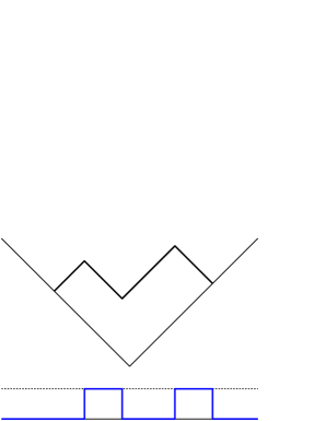
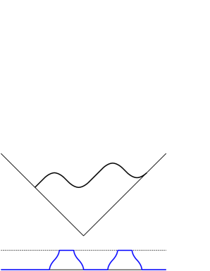
(a) Ground state		(b) Douglas-Kazakov phase
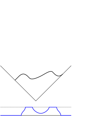
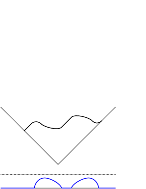
(c) Gross-Witten phase		(d) Matrix model phase

Figure 5: Various phases in the continuum limit of the discrete matrix model. Here we show a two-cuts solution for instance.

From these observations, we notice that the following important fact: If we exchange a role of the right-down and right-up edge in the Young diagram, or correspondingly, the positions of eigenvalues (electron) and vacuums (hall), the Douglas-Kazakov phase transition and the Gross-Witten phase transition exchange each other. In this sense, these phase transitions are essentially the same phenomena and are dual under the above operation.

Finally, we comment on the relation to the Nekrasov’s instanton partition function and Dijkgraaf-Vafa theory. As we discussed in section 3, we need to take a suitable double scaling large $N$ limit in order to obtain the instanton partition function from the discrete matrix model (${{\rm gYM}_{2}}$). In this limit, the chiral decomposition is also needed. To decompose the partition function into two parts, we assume the melting of the corner of the Young diagram is sufficiently small comparing with the planar right-down edge. We have scaled up the planar region and decoupled the two fermi surface with each other. Namely, we need to take the large $N$ limit at least in the phase (b). The scaled-up melting corner of one of the fermi surface will correspond to the limiting shape of the instanton partition function. On the other hand, the holomorphic matrix model using in the Dijkgraaf-Vafa theory does not have the Douglas-Kazakov type phase transition since there is no upper limitation in the eigenvalue densities. So all eigenvalue densities have the semi-circle shape. Thus, we find the Dijkgraaf-Vafa analysis is valid only for the phase (d). We need to take the large $N$ and continuum limit in this phase to get the effective superpotential of ${\cal N}{=}1$ theories.

We can obtain all order graviphoton corrections for the ${\cal N}{=}2$ prepotential from an asymptotic expansion of Nekrasov’s formula. It however is still difficult to obtain all order graviphoton correction for the superpotential of ${\cal N}{=}1$ theory since we need sub-leading terms in the $1/N$ expansion of the random matrix models, where we can not use the WKB (saddle point) approximation. The discretization of the random matrix model seems to connect the two approaches by Nekrasov and Dijkgraaf-Vafa. We expect that our observation sheds new lights on the exact relation between them and gives a new closed formula for the effective superpotential of ${\cal N}{=}1$ theory which gives all graviphoton corrections as the asymptotic expansion like Nekrasov’s formula, beyond the correspondence between ${\cal N}{=}2$ and ${\cal N}{=}1$ theories at the algebraic geometry (curve) level [48].

Appendix A Generalized $\zeta$-function and perturbative contribution

The perturbative contribution to the partition function is obtained essentially from infinite products,

$$\prod_{(i,j)\in\mathbb{N}^{2}}(a_{l}-a_{n}+g_{s}(j-i)),$$ (A.1)

where $\mathbb{N}$ is a set of natural numbers (non-zero positive integers). This type of the infinite product can be understood as the determinant of an operator (the product of eigenvalue spectra). This infinite product can be evaluated by using the $\zeta$-function regularization technique.

We define the generalized $\zeta$-function as

$$\zeta_{\vec{\epsilon}}(s;x)\equiv\sum_{\vec{n}\in\mathbb{N}^{d}}\frac{1}{(x+\vec{\epsilon}\cdot\vec{n})^{s}},$$ (A.2)

where $\epsilon=(\epsilon_{1},\epsilon_{2},\ldots,\epsilon_{d})$ is a vector of parameters and $n=(n_{1},n_{2},\ldots,n_{d})$ is a set of non-zero positive integers. Using this $\zeta$-function, the logarithm of infinite products like (A.1) can be expressed as

$$\log\prod_{\vec{n}\in\mathbb{N}^{d}}(x+\vec{\epsilon}\cdot\vec{n}) = \sum_{\vec{n}\in\mathbb{N}^{d}}\log(x+\vec{\epsilon}\cdot\vec{n})$$ (A.3)

$$= -\left.\frac{d}{ds}\zeta_{\vec{\epsilon}}(s;x)\right|_{s\rightarrow 0}.$$

Multiplying the gamma function,

$$\Gamma(s)=\int_{0}^{\infty}u^{s-1}e^{-u}du,$$ (A.4)

by $\zeta_{\vec{\epsilon}}(s;x)$, we find

$$\Gamma(s)\zeta_{\vec{\epsilon}}(s;x)=\sum_{\vec{n}\in\mathbb{Z}_{+}^{d}}\int_{0}^{\infty}du(x+\vec{\epsilon}\cdot\vec{n})^{-s}u^{s-1}e^{-u}.$$ (A.5)

After changing variable by $u=t(x+\vec{\epsilon}\cdot\vec{n})$, we obtain

$$\zeta_{\vec{\epsilon}}(s;x) = \frac{1}{\Gamma(s)}\int_{0}^{\infty}\frac{dt}{t}t^{s}\sum_{\vec{n}\in\mathbb{Z}_{+}^{d}}e^{-(x+\vec{\epsilon}\cdot\vec{n})t}$$ (A.6)

$$= \frac{1}{\Gamma(s)}\int_{0}^{\infty}\frac{dt}{t}t^{s}\frac{e^{-tx}}{\prod_{i=1}^{d}(e^{\epsilon_{i}t}-1)}.$$

Especially, in the case of (A.1), we have

$$\prod_{(i,j)\in\mathbb{N}^{2}}(a_{l}-a_{n}+g_{s}(j-i))=e^{-\gamma_{g_{s}}(a_{l}-a_{n})},$$ (A.7)

where

$$\gamma_{g_{s}}(x)=-\left.\frac{d}{ds}\left(\frac{1}{\Gamma(s)}\int_{0}^{\infty}\frac{dt}{t}t^{s}\frac{e^{-tx}}{(e^{g_{s}t}-1)(e^{-g_{s}t}-1)}\right)\right|_{s\rightarrow 0}.$$ (A.8)

It is easy to find from this expression to show that it satisfies the difference equation,

$$\gamma_{g_{s}}(x+g_{s})+\gamma_{g_{s}}(x-g_{s})-2\gamma_{g_{s}}(x)=\log x,$$ (A.9)

and that the series expansion with respect to $g_{s}$ becomes

$$\gamma_{g_{s}}(x)=\sum_{g}g_{s}^{2g-2}f_{g}(x),$$ (A.10)

with

$$\begin{split}&f_{0}(x)=\frac{1}{2}x^{2}\log x-\frac{3}{4}x^{2},\\ &f_{1}(x)=-\frac{1}{12}\log x,\\ &f_{2}(x)=-\frac{1}{240}\frac{1}{x^{2}},\\ &\qquad\vdots\\ &f_{g}(x)=\frac{B_{2g}}{2g(2g-2)x^{2g-2}}.\end{split}$$ (A.11)

References

• [1] N. Nekrasov and A. Okounkov, Seiberg-Witten theory and random partitions, hep-th/0306238.
• [2] R. Dijkgraaf and C. Vafa, Matrix models, topological strings, and supersymmetric gauge theories, Nucl. Phys. B644 (2002) 3–20 [hep-th/0206255].
• [3] R. Dijkgraaf and C. Vafa, On geometry and matrix models, Nucl. Phys. B644 (2002) 21–39 [hep-th/0207106].
• [4] R. Dijkgraaf and C. Vafa, A perturbative window into non-perturbative physics, hep-th/0208048.
• [5] T. Matsuo, S. Matsuura and K. Ohta, Large N limit of 2D Yang-Mills theory and instanton counting, hep-th/0406191.
• [6] A. Okounkov, N. Reshetikhin and C. Vafa, Quantum Calabi-Yau and classical crystals, hep-th/0309208.
• [7] A. Iqbal, N. Nekrasov, A. Okounkov and C. Vafa, Quantum foam and topological strings, hep-th/0312022.
• [8] R. Gopakumar and C. Vafa, Topological gravity as large N topological gauge theory, Adv. Theor. Math. Phys. 2 (1998) 413–442 [hep-th/9802016].
• [9] R. Gopakumar and C. Vafa, On the gauge theory/geometry correspondence, Adv. Theor. Math. Phys. 3 (1999) 1415–1443 [hep-th/9811131].
• [10] A. Gorsky and A. Mironov, Integrable many-body systems and gauge theories, hep-th/0011197.
• [11] T. J. Hollowood, Critical points of glueball superpotentials and equilibria of integrable systems, JHEP 10 (2003) 051 [hep-th/0305023].
• [12] M. Bershadsky, C. Vafa and V. Sadov, D-Branes and Topological Field Theories, Nucl. Phys. B463 (1996) 420–434 [hep-th/9511222].
• [13] E. Witten, Two-dimensional gauge theories revisited, J. Geom. Phys. 9 (1992) 303–368 [hep-th/9204083].
• [14] G. W. Moore, N. Nekrasov and S. Shatashvili, Integrating over Higgs branches, Commun. Math. Phys. 209 (2000) 97–121 [hep-th/9712241].
• [15] O. Ganor, J. Sonnenschein and S. Yankielowicz, The String theory approach to generalized 2-D Yang-Mills theory, Nucl. Phys. B434 (1995) 139–178 [hep-th/9407114].
• [16] R. Dijkgraaf and C. Vafa, N = 1 supersymmetry, deconstruction, and bosonic gauge theories, hep-th/0302011.
• [17] C. Vafa, Two dimensional Yang-Mills, black holes and topological strings, hep-th/0406058.
• [18] M. Aganagic, H. Ooguri, N. Saulina and C. Vafa, Black holes, q-deformed 2d Yang-Mills, and non-perturbative topological strings, hep-th/0411280.
• [19] M. Blau and G. Thompson, Derivation of the Verlinde formula from Chern-Simons theory and the G/G model, Nucl. Phys. B408 (1993) 345–390 [hep-th/9305010].
• [20] M. Blau and G. Thompson, Lectures on 2-d gauge theories: Topological aspects and path integral techniques, hep-th/9310144.
• [21] A. A. Migdal, Recursion equations in gauge field theories, Sov. Phys. JETP 42 (1975) 413.
• [22] T. Maeda, T. Nakatsu, K. Takasaki and T. Tamakoshi, Free fermion and Seiberg-Witten differential in random plane partitions, hep-th/0412329.
• [23] D. J. Gross and I. Taylor, Washington, Two-dimensional QCD is a string theory, Nucl. Phys. B400 (1993) 181–210 [hep-th/9301068].
• [24] D. J. Gross and I. Taylor, Washington, Twists and Wilson loops in the string theory of two- dimensional QCD, Nucl. Phys. B403 (1993) 395–452 [hep-th/9303046].
• [25] D. J. Gross and W. Taylor, Two-dimensional QCD and strings, hep-th/9311072.
• [26] S. Cordes, G. W. Moore and S. Ramgoolam, Lectures on 2-d Yang-Mills theory, equivariant cohomology and topological field theories, Nucl. Phys. Proc. Suppl. 41 (1995) 184–244 [hep-th/9411210].
• [27] U. Bruzzo, F. Fucito, J. F. Morales and A. Tanzini, Multi-instanton calculus and equivariant cohomology, JHEP 05 (2003) 054 [hep-th/0211108].
• [28] F. Fucito, J. F. Morales and R. Poghossian, Instantons on quivers and orientifolds, JHEP 10 (2004) 037 [hep-th/0408090].
• [29] M. R. Douglas and V. A. Kazakov, Large N phase transition in continuum QCD in two- dimensions, Phys. Lett. B319 (1993) 219–230 [hep-th/9305047].
• [30] D. J. Gross and E. Witten, POSSIBLE THIRD ORDER PHASE TRANSITION IN THE LARGE N LATTICE GAUGE THEORY, Phys. Rev. D21 (1980) 446–453.
• [31] S. Katz, A. Klemm and C. Vafa, Geometric engineering of quantum field theories, Nucl. Phys. B497 (1997) 173–195 [hep-th/9609239].
• [32] S. Katz, P. Mayr and C. Vafa, Mirror symmetry and exact solution of 4D N = 2 gauge theories. I, Adv. Theor. Math. Phys. 1 (1998) 53–114 [hep-th/9706110].
• [33] A. Hanany and E. Witten, Type IIB superstrings, BPS monopoles, and three-dimensional gauge dynamics, Nucl. Phys. B492 (1997) 152–190 [hep-th/9611230].
• [34] E. Witten, Solutions of four-dimensional field theories via M-theory, Nucl. Phys. B500 (1997) 3–42 [hep-th/9703166].
• [35] N. Nekrasov and A. Schwarz, Instantons on noncommutative R**4 and (2,0) superconformal six dimensional theory, Commun. Math. Phys. 198 (1998) 689–703 [hep-th/9802068].
• [36] N. A. Nekrasov, Seiberg-Witten prepotential from instanton counting, hep-th/0206161.
• [37] T. Eguchi and H. Kawai, Reduction of Dynamical Degrees of Freedom in the Large N Gauge Theory, Phys. Rev. Lett. 48 (1982) 1063.
• [38] N. Ishibashi, H. Kawai, Y. Kitazawa and A. Tsuchiya, A large-N reduced model as superstring, Nucl. Phys. B498 (1997) 467–491 [hep-th/9612115].
• [39] N. Seiberg, A note on background independence in noncommutative gauge theories, matrix model and tachyon condensation, JHEP 09 (2000) 003 [hep-th/0008013].
• [40] E. Witten, TOPOLOGICAL QUANTUM FIELD THEORY, Commun. Math. Phys. 117 (1988) 353.
• [41] D. J. Gross, Two-dimensional QCD as a string theory, Nucl. Phys. B400 (1993) 161–180 [hep-th/9212149].
• [42] H. Ooguri and C. Vafa, Worldsheet derivation of a large N duality, Nucl. Phys. B641 (2002) 3–34 [hep-th/0205297].
• [43] A. S. Losev, A. Marshakov and N. A. Nekrasov, Small instantons, little strings and free fermions, hep-th/0302191.
• [44] T. Maeda, T. Nakatsu, K. Takasaki and T. Tamakoshi, Five-dimensional supersymmetric Yang-Mills theories and random plane partitions, JHEP 03 (2005) 056 [hep-th/0412327].
• [45] A. Kapustin and S. Sethi, The Higgs branch of impurity theories, Adv. Theor. Math. Phys. 2 (1998) 571–591 [hep-th/9804027].
• [46] R. Donagi and E. Witten, Supersymmetric Yang-Mills Theory And Integrable Systems, Nucl. Phys. B460 (1996) 299–334 [hep-th/9510101].
• [47] D. J. Gross and A. Matytsin, Some properties of large N two-dimensional Yang-Mills theory, Nucl. Phys. B437 (1995) 541–584 [hep-th/9410054].
• [48] F. Cachazo and C. Vafa, N = 1 and N = 2 geometry from fluxes, hep-th/0206017.