Introduction to the Gribov Ambiguities In Euclidean Yang-Mills Theories

Abstract

An introduction to the Gribov ambiguities and their consequences on the infrared behavior of Euclidean Yang-Mills theories is presented.

1 Introduction

Nowadays, that the Gribov ambiguities play an important role in the quantization of Yang-Mills theories is becoming more and more evident. These ambiguities, affecting the Faddeev-Popov quantization formula, deeply modify the infrared behavior of the theory and might have a crucial role in the understanding of color confinement.

The aim of these notes is to give a simple introduction to Gribov’s work and to its consequences on the infrared regime of nonabelian Euclidean gauge theories. The discussion will be focused mainly on the original paper by Gribov [1], whose content will be reproduced in a somewhat detailed way.

This work is divided in two parts. Part I is devoted to the study of the Gribov ambiguities. We begin by reviewing the examples provided by Gribov [1]. Further, a class of Gribov copies proposed by Henyey [2] will be considered.

In Part II we introduce the so called Gribov horizons and we analyze their properties. Following Gribov’s suggestion, the restriction of the domain of integration in the Feynman path integral to the first horizon will be discussed. The ensuing modifications on the infrared behavior of the gluon and ghost propagators in the Landau gauge will be worked out.

We conclude this short introduction by mentioning a result due to Singer [3]. Although the examples of the Gribov copies which we shall consider in the following will be worked out in the transverse gauge, $\partial A=0$, the existence of the Gribov ambiguities is not related to a specific gauge condition. As pointed out in [3], the presence of Gribov copies is in fact a general feature of nonabelian gauge theories.

2 Part I: The Gribov Pendulum

2.1 The Gribov ambiguities

2.1.1 Quantization of Euclidean Yang-Mills theories. Non-uniqueness of the gauge condition

The Euclidean Yang-Mills action

$$S_{YM}=\frac{1}{4g^{2}}\int{d^{4}x}F_{\mu\nu}^{a}F_{\mu\nu}^{a}\;,$$ (1)

is left invariant if one replaces $A_{\mu}$ by the gauge transformed field $\widetilde{A}_{\mu}$

$$A_{\mu}\rightarrow\widetilde{A}_{\mu}={S}^{\dagger}\partial_{\mu}{S}+S^{\dagger}A_{\mu}{S}\;.$$ (2)

The fields $A_{\mu}$ and $\widetilde{A}_{\mu}$ define equivalent configurations, leading to the same value for the expression $\left(\ref{eq1}\right)$. In order to properly quantize the theory, only inequivalent configurations should be taken into account in the Feynman path integral. The first step towards the implementation of this procedure is provided by the Faddeev-Popov quantization formula. One integrates over configurations which have a certain divergence, i.e.

$$\partial_{\mu}A_{\mu}=f\;.$$ (3)

Therefore, for the partition function one gets

$$\mathcal{Z=N}\int DA_{\mu}\delta(\partial A-f)\mathrm{\det}\left(\mathcal{M}^{ab}(A)\right)e^{-\frac{1}{4g^{2}}\int{d^{4}x}F_{\mu\nu}^{a}F_{\mu\nu}^{a}\;}\;,$$ (4)

where

$$\mathcal{M}^{ab}(A)=-\partial_{\mu}(\partial_{\mu}\delta^{ab}-f^{abc}A_{\mu}^{c})\;,$$ (5)

is the Faddeev-Popov operator and $\mathcal{N}$ a normalization factor. In the following we shall limit ourselves to the choice $f=0$, which amounts to impose the following transversality condition

$$\partial A=0\;.$$ (6)

This condition is known as the Landau gauge condition. Thus

$$\mathcal{Z=N}\int DA_{\mu}\delta(\partial A)\mathrm{\det}\left(\mathcal{M}^{ab}\right)e^{-\frac{1}{4g^{2}}\int{d^{4}x}F_{\mu\nu}^{a}F_{\mu\nu}^{a}\;}\;.$$ (7)

However, as pointed out by Gribov [1], the condition $\partial A=0$ does not fix uniquely the gauge configurations. This means that, for a given $A_{\mu}$ satisfying the gauge condition $\partial A=0$, there exist equivalent fields $\widetilde{A}_{\mu}$ obeying the same condition, i.e.

$$\widetilde{A}_{\mu} = {S}^{\dagger}\partial_{\mu}{S}+S^{\dagger}A_{\mu}{S}=A_{\mu}+S^{\dagger}(\partial_{\mu}S+[A_{\mu},S])\;,$$

$$\partial\widetilde{A} = \partial A=0\;.$$ (8)

Field configurations $\widetilde{A}_{\mu}$ satisfying the conditions $\left(\ref{eq8}\right)$ are copies of $A_{\mu}$. In terms of the gauge transformation $S$, the condition $\partial\widetilde{A}=\partial A=0$ reads

$$\partial_{\mu}(S^{\dagger}(\partial_{\mu}S+[A_{\mu},S]))=0\;,$$ (9)

which, due to $\partial A=0$, becomes

$$\partial_{\mu}S^{\dagger}\partial_{\mu}{S+S}^{\dagger}\partial_{\mu}\partial_{\mu}{S+\partial}_{\mu}S^{\dagger}A_{\mu}{S+}S^{\dagger}A_{\mu}{\partial}_{\mu}{S=0\;.}$$ (10)

• Remark

  At the infinitesimal level, $S=1+\alpha,$ $\alpha\ll 1$, expression $\left(\ref{eq10}\right)$ reduces to

  $$\partial^{2}\alpha-(\partial_{\mu}\alpha)A_{\mu}+A_{\mu}(\partial_{\mu}\alpha)=0\;,$$ (11)

  i.e.

  $$\partial_{\mu}\left(\partial_{\mu}\alpha+\left[A_{\mu},\alpha\right]\right)=0\;.$$ (12)

  We see that, in the infinitesimal case, the condition for the existence of Gribov’s copies is equivalent to state that the operator $-\partial_{\mu}\left(\partial_{\mu}\cdot+\left[A_{\mu},\cdot\right]\right)$, whose determinant enters the Faddeev-Popov quantization formula $\left(\ref{eq7}\right)$, has zero eigenvalues. Notice that the eigenvalues equation for the Faddeev-Popov operator $-\partial_{\mu}\left(\partial_{\mu}\cdot+\left[A_{\mu},\cdot\right]\right)$,

  $$-\partial_{\mu}\left(\partial_{\mu}\psi+\left[A_{\mu},\psi\right]\right)=\epsilon(A)\psi\;,$$ (13)

  can be seen as a kind of Schrödinger equation, with $A_{\mu}$ playing the role of the potential. Therefore, for large enough values of the field $A_{\mu}$, we might expect that zero energy solutions, $\epsilon=0$, of eq.$\left(\ref{eq13}\right)$ do in fact exist.

2.1.2 The Gribov pendulum

In order to analyze the condition for the existence of Gribov’s copies, we shall consider the three-dimensional case, $A_{i}$,$\;i=1,2,3$, assuming that the gauge group is $SU(2)$ and that the gauge field is spherically symmetric, i.e. $A_{i}$ depends on the unit vector $n_{i}=x_{i}/r$, $r=\sqrt{x_{i}x_{i}}$, $n_{i}n_{i}=1$. Let $\sigma_{i}$ denote the $2\times 2$ Pauli matrices

$$\sigma_{i}\sigma_{j}=\delta_{ij}+i\varepsilon_{ijk}\sigma_{k}\;.$$ (14)

$$\sigma_{1}=\left(\begin{array}[]{ll}0&1\\ 1&0\end{array}\right),\;\;\;\;\sigma_{2}=\left(\begin{array}[]{ll}0&i\\ -i&0\end{array}\right),\;\;\;\;\sigma_{3}=\left(\begin{array}[]{ll}1&0\\ 0&-1\end{array}\right)\;.$$ (15)

It follows that the quantity $\widehat{n}$

$$\widehat{n}=in_{i}\sigma_{i}\;,$$ (16)

obeys

$$\widehat{n}^{2}=-n_{i}n_{j}\sigma_{i}\sigma_{j}=-n_{i}n_{i}=-1\;.$$ (17)

Since the gauge field $A_{i}$ is Lie algebra valued, it can be parametrized as

$$A_{i}=a_{1}(r)In_{i}+a_{2}(r)\sigma_{i}+a_{3}(r)n_{i}(\overrightarrow{n}\cdot\overrightarrow{\sigma})+a_{4}(r)\sigma_{i}(\overrightarrow{n}\cdot\overrightarrow{\sigma})\;,$$ (18)

where $I$ stands for the $2\times 2$ unit matrix and where we have taken into account that $A_{i}$ is spherically symmetric. Notice that, due to $n_{i}n_{i}=1$, and $(\overrightarrow{n}\cdot\overrightarrow{\sigma})^{2}=1$, higher powers of $\left(n_{i}n_{i}\right)^{n}$ and $(\overrightarrow{n}\cdot\overrightarrow{\sigma})^{m}$ are absent in the expression $\left(\ref{eq17}\right)$. Also, we observe that

$$i\varepsilon_{ijk}n_{j}\sigma_{k}=n_{j}\left(\sigma_{i}\sigma_{j}-\delta_{ij}\right)=\sigma_{i}(\overrightarrow{n}\cdot\overrightarrow{\sigma})-n_{i}\;,$$ (19)

meaning that this term is not independent. In addition, from eq.$\left(\ref{eq14}\right)$, it follows that

$$(\overrightarrow{n}\cdot\overrightarrow{\sigma})\sigma_{i}=-\sigma_{i}(\overrightarrow{n}\cdot\overrightarrow{\sigma})+2n_{i}\;.$$ (20)

Thus, expression $\left(\ref{eq17}\right)$ yields the most general form for a $SU(2)$ field which is spherically symmetric. Moreover, due to the traceless condition

$$Tr\sigma^{a}A_{i}^{a}=0\;,$$

we get the relationship

$$a_{4}=-a_{1}\;,$$ (21)

so that $A_{i}$ turns out to be parametrized by three independent quantities

$$A_{i}=a_{1}(r)In_{i}+a_{2}(r)\sigma_{i}+a_{3}(r)n_{i}(\overrightarrow{n}\cdot\overrightarrow{\sigma})-a_{1}(r)\sigma_{i}(\overrightarrow{n}\cdot\overrightarrow{\sigma})\;.$$ (22)

Of course, we can adopt the same parametrization employed by Gribov [1], namely

$$A_{i}=f_{1}(r)\frac{\partial\widehat{n}}{\partial x_{i}}+f_{2}(r)\widehat{n}\frac{\partial\widehat{n}}{\partial x_{i}}+f_{3}(r)\widehat{n}n_{i}\;.$$ (23)

Indeed, from

$$\frac{\partial\widehat{n}}{\partial x_{i}}=\frac{i}{r}\sigma_{k}(\delta_{ik}-n_{i}n_{k})=\frac{i}{r}\left(\sigma_{i}-(\overrightarrow{n}\cdot\overrightarrow{\sigma})n_{i}\right)\;,$$ (24)

it follows

$$A_{i}=\frac{i}{r}f_{1}(r)\sigma_{i}-\frac{i}{r}f_{1}(r)(\overrightarrow{n}\cdot\overrightarrow{\sigma})n_{i}-\frac{1}{r}f_{2}(r)(\overrightarrow{n}\cdot\overrightarrow{\sigma})\sigma_{i}+\frac{1}{r}f_{2}(r)n_{i}+if_{3}(r)(\overrightarrow{n}\cdot\overrightarrow{\sigma})n_{i}\;$$ (25)

which has precisely the same form of expression $\left(\ref{eq21}\right)$.

• Observe that for $f_{1}=f_{3}=0$, expression $\left(\ref{eq22}\right)$ becomes

  $$A_{i} = -\frac{1}{r}f_{2}(r)(\overrightarrow{n}\cdot\overrightarrow{\sigma})\sigma_{i}+\frac{1}{r}f_{2}(r)n_{i}\;$$

  $$= -\frac{1}{r}f_{2}(r)\left(\delta_{ij}+i\varepsilon_{jik}\sigma_{k}\right)n_{j}+\frac{1}{r}f_{2}(r)n_{i}$$

  $$= \frac{i}{r^{2}}\varepsilon_{ijk}x_{j}\sigma_{k}f_{2}(r)\;,$$

  which is purely transverse, i.e.

  $$\partial_{i}A_{i}=0\;.$$ (27)

Having found the most general parametrization for the $SU(2)$ gauge field, eq.$\left(\ref{eq22}\right)$, let us work out the condition for the existence of copies, i.e.

$$\widetilde{A}_{i} = {S}^{\dagger}\partial_{i}{S}+S^{\dagger}A_{i}{S\;,}$$ (28)

$$\partial_{i}\widetilde{A}_{i} = \partial_{i}A_{i}\;,$$

where we shall consider the class of gauge transformations $S$ parametrized by

$$S=e^{\frac{i}{2}\alpha(r)\overrightarrow{n}\cdot\overrightarrow{\sigma}}=\cos\frac{\alpha(r)}{2}+i\overrightarrow{n}\cdot\overrightarrow{\sigma}\sin\frac{\alpha(r)}{2}\;.$$ (29)

From eqs.$\left(\ref{eq27}\right)$, $\left(\ref{eq28}\right)$ it follows

$$\widetilde{A}_{i} = \left(\cos\frac{\alpha}{2}-\widehat{n}\sin\frac{\alpha}{2}\right)\left[\left(-\sin\frac{\alpha}{2}+\widehat{n}\cos\frac{\alpha}{2}\right)\frac{1}{2}\frac{\partial\alpha}{\partial x_{i}}+\;\sin\frac{\alpha}{2}\frac{\partial\widehat{n}}{\partial x_{i}}\right]$$

$$+\left(\cos\frac{\alpha}{2}-\widehat{n}\sin\frac{\alpha}{2}\right)\left(f_{1}(r)\frac{\partial\widehat{n}}{\partial x_{i}}+f_{2}(r)\widehat{n}\frac{\partial\widehat{n}}{\partial x_{i}}+f_{3}(r)\widehat{n}n_{i}\right)\left(\cos\frac{\alpha}{2}+\widehat{n}\sin\frac{\alpha}{2}\right)$$

$$= \left(\widehat{n}\cos^{2}\frac{\alpha}{2}+\widehat{n}\sin^{2}\frac{\alpha}{2}\right)\frac{1}{2}\frac{\partial\alpha}{\partial x_{i}}+\cos\frac{\alpha}{2}\sin\frac{\alpha}{2}\frac{\partial\widehat{n}}{\partial x_{i}}-\sin^{2}\frac{\alpha}{2}\widehat{n}\frac{\partial\widehat{n}}{\partial x_{i}}$$

$$+\left(f_{1}\cos\frac{\alpha}{2}\frac{\partial\widehat{n}}{\partial x_{i}}+f_{2}\cos\frac{\alpha}{2}\widehat{n}\frac{\partial\widehat{n}}{\partial x_{i}}+f_{3}\cos\frac{\alpha}{2}\widehat{n}n_{i}-f_{1}\sin\frac{\alpha}{2}\widehat{n}\frac{\partial\widehat{n}}{\partial x_{i}}\right.$$

$$\left.+f_{2}\sin\frac{\alpha}{2}\frac{\partial\widehat{n}}{\partial x_{i}}+f_{3}\sin\frac{\alpha}{2}n_{i}\right)\left(\cos\frac{\alpha}{2}+\widehat{n}\sin\frac{\alpha}{2}\right)\;.$$

Since

$$\frac{\partial\alpha}{\partial x_{i}}=\alpha^{\prime}(r)n_{i}\;,$$ (31)

we obtain

$$\widetilde{A}_{i} = \frac{1}{2}\alpha^{\prime}(r)\widehat{n}n_{i}+\frac{1}{2}\sin\alpha\frac{\partial\widehat{n}}{\partial x_{i}}-\sin^{2}\frac{\alpha}{2}\widehat{n}\frac{\partial\widehat{n}}{\partial x_{i}}$$ (32)

$$+f_{1}\left(\cos^{2}\frac{\alpha}{2}\frac{\partial\widehat{n}}{\partial x_{i}}+\cos\frac{\alpha}{2}\sin\frac{\alpha}{2}\left[\frac{\partial\widehat{n}}{\partial x_{i}},\widehat{n}\right]-\sin^{2}\frac{\alpha}{2}\widehat{n}\frac{\partial\widehat{n}}{\partial x_{i}}\widehat{n}\right)$$

$$+f_{2}\left(\cos^{2}\frac{\alpha}{2}\widehat{n}\frac{\partial\widehat{n}}{\partial x_{i}}+\cos\frac{\alpha}{2}\sin\frac{\alpha}{2}\widehat{n}\frac{\partial\widehat{n}}{\partial x_{i}}\widehat{n}+\cos\frac{\alpha}{2}\sin\frac{\alpha}{2}\frac{\partial\widehat{n}}{\partial x_{i}}+\sin^{2}\frac{\alpha}{2}\frac{\partial\widehat{n}}{\partial x_{i}}\widehat{n}\right)$$

$$+f_{3}\widehat{n}n_{i}\;.$$

Observing that

$$\frac{\partial n_{k}}{\partial x_{i}}n_{j}(\sigma_{k}\sigma_{j}+\sigma_{j}\sigma_{k})=2\frac{\partial n_{k}}{\partial x_{i}}n_{j}\delta_{kj}=2\frac{\partial n_{k}}{\partial x_{i}}n_{k}=\frac{\partial\left(n_{k}n_{k}\right)}{\partial x_{i}}=0\;,$$ (33)

one has

$$\frac{\partial\widehat{n}}{\partial x_{i}}\widehat{n}=-\widehat{n}\frac{\partial\widehat{n}}{\partial x_{i}}\;,$$ (34)

and

$$\widehat{n}\frac{\partial\widehat{n}}{\partial x_{i}}\widehat{n}=-\widehat{n}\widehat{n}\frac{\partial\widehat{n}}{\partial x_{i}}=\frac{\partial\widehat{n}}{\partial x_{i}}\;.$$ (35)

Therefore

$$\widetilde{A}_{i} = \left(f_{1}\left(\cos^{2}\frac{\alpha}{2}-\sin^{2}\frac{\alpha}{2}\right)+2f_{2}\cos\frac{\alpha}{2}\sin\frac{\alpha}{2}\right)\frac{\partial\widehat{n}}{\partial x_{i}}$$

$$+\left(f_{2}\left(\cos^{2}\frac{\alpha}{2}-\sin^{2}\frac{\alpha}{2}\right)-2f_{1}\cos\frac{\alpha}{2}\sin\frac{\alpha}{2}\right)\widehat{n}\frac{\partial\widehat{n}}{\partial x_{i}}$$

$$+\left(f_{3}+\frac{1}{2}\alpha^{\prime}(r)\right)\widehat{n}n_{i}+\frac{1}{2}\sin\alpha\frac{\partial\widehat{n}}{\partial x_{i}}-\frac{1}{2}\left(1-\cos\alpha\right)\widehat{n}\frac{\partial\widehat{n}}{\partial x_{i}}\;.$$

Finally, recalling that

$$\cos^{2}\frac{\alpha}{2}-\sin^{2}\frac{\alpha}{2} = \cos\alpha\;,$$ (37)

$$2\cos\frac{\alpha}{2}\sin\frac{\alpha}{2} = \sin\alpha\;,$$

we get

$$\widetilde{A}_{i} = \left(f_{1}\cos\alpha+\left(f_{2}+\frac{1}{2}\right)\sin\alpha\right)\frac{\partial\widehat{n}}{\partial x_{i}}$$ (38)

$$+\left(\left(f_{2}+\frac{1}{2}\cos\alpha\right)-f_{1}\sin\alpha-\frac{1}{2}\right)\widehat{n}\frac{\partial\widehat{n}}{\partial x_{i}}+\left(f_{3}+\frac{1}{2}\alpha^{\prime}(r)\right)\widehat{n}n_{i}\;.$$

It remains now to work out the condition $\partial_{i}\widetilde{A}_{i}=\partial_{i}A_{i}$. After a little algebra, one obtains the differential equation

$$\alpha^{\prime\prime}(r)+\frac{2}{r}\alpha^{\prime}(r)-\frac{4}{r^{2}}\left(\left(f_{2}+\frac{1}{2}\right)\sin\alpha+f_{1}\left(\cos\alpha-1\right)\right)=0\;.$$ (39)

Setting

$$\tau=\log r\;,{\ }{\ }{\ }{\ }r=e^{\tau}\;,$$

equation $\left(\ref{eq38}\right)$ becomes

$$\frac{\partial^{2}\alpha(\tau)}{\partial\tau^{2}}+\frac{\partial\alpha(\tau)}{\partial\tau}-4\left(\left(f_{2}+\frac{1}{2}\right)\sin\alpha+f_{1}\left(\cos\alpha-1\right)\right)=0\;,$$ (40)

which is the equation of a pendulum in the presence of a damping term $\alpha^{\prime}(\tau)$, see Fig.1.

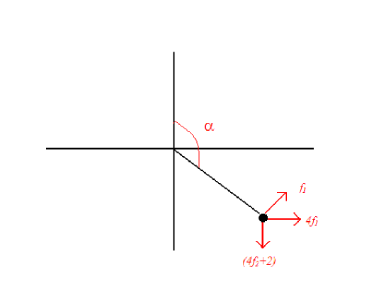
Figure 1: The Gribov pendulum

• Summary

  We have started with the most general spherically symmetric $SU(2)$ field

  $$A_{i}=f_{1}(r)\frac{\partial\widehat{n}}{\partial x_{i}}+f_{2}(r)\widehat{n}\frac{\partial\widehat{n}}{\partial x_{i}}+f_{3}(r)\widehat{n}n_{i}\;.$$ (41)

  For the gauge transformed field

  $$\widetilde{A}_{i} = {S}^{\dagger}\partial_{i}{S}+S^{\dagger}A_{i}{S\;,}$$ (42)

  $$S = e^{\frac{i}{2}\alpha(r)\overrightarrow{n}\cdot\overrightarrow{\sigma}}=\cos\frac{\alpha}{2}+i\overrightarrow{n}\cdot\overrightarrow{\sigma}\sin\frac{\alpha}{2}\;,$$

  we have

  $$\widetilde{A}_{i} = \widetilde{f_{1}}(r)\frac{\partial\widehat{n}}{\partial x_{i}}+\widetilde{f_{2}}(r)\widehat{n}\frac{\partial\widehat{n}}{\partial x_{i}}+\widetilde{f_{3}}(r)\widehat{n}n_{i}\;,$$ (43)

  $$\widetilde{f_{1}}(r) = f_{1}\cos\alpha+\left(f_{2}+\frac{1}{2}\right)\sin\alpha\;,$$

  $$\widetilde{f_{2}}(r) = f_{2}+\frac{1}{2}\cos\alpha-f_{1}\sin\alpha-\frac{1}{2}\;,$$

  $$\widetilde{f_{3}}(r) = f_{3}+\frac{1}{2}\alpha^{\prime}(r)\;.$$

  Finally, the condition $\partial_{i}\widetilde{A}_{i}=\partial_{i}A_{i}$ yields

  $$\frac{\partial^{2}\alpha(\tau)}{\partial\tau^{2}}+\frac{\partial\alpha(\tau)}{\partial\tau}-4\left(\left(f_{2}+\frac{1}{2}\right)\sin\alpha+f_{1}\left(\cos\alpha-1\right)\right)=0\;.$$ (44)

  This is the equation of a pendulum in the presence of a damping term $\alpha^{\prime}(\tau)$. The components $f_{1},f_{2}$ of the gauge field $\left(\ref{eq40}\right)$ correspond to the forces acting on the pendulum, Fig.1, see also Appendix B.

2.2 Examples of Gribov’s copies

In this section we shall work out explicit examples of Gribov’s copies. We shall restrict ourselves to the transversality condition

$$\partial_{i}\widetilde{A}_{i}=\partial_{i}A_{i}=0\;.$$ (45)

As initial gauge configuration we shall take

$$A_{i}=\frac{i}{r^{2}}\varepsilon_{ijk}x_{j}\sigma_{k}f(r)\;,\;\;\;\;\partial_{i}A_{i}=0\;,\;\;\;$$ (46)

corresponding to setting $f_{1}=f_{3}=0$, $f_{2}=f$ in expression $\left(\ref{eq40}\right)$. The gauge transformed field, eq.$\left(\ref{eq41}\right)$, is given by

$$\widetilde{A}_{i}=\left(f+\frac{1}{2}\right)\sin\alpha\frac{\partial\widehat{n}}{\partial x_{i}}+\left(f+\frac{1}{2}\cos\alpha-\frac{1}{2}\right)\widehat{n}\frac{\partial\widehat{n}}{\partial x_{i}}+\frac{1}{2}\alpha^{\prime}(r)\widehat{n}n_{i}\;.$$ (47)

Also, the condition $\partial_{i}\widetilde{A}_{i}=0$, gives

$$\alpha^{\prime\prime}(r)+\frac{2}{r}\alpha^{\prime}(r)-\frac{4}{r^{2}}\left(f+\frac{1}{2}\right)\sin\alpha=0\;,$$ (48)

or, $\tau=\log r$,

$$\frac{\partial^{2}\alpha(\tau)}{\partial\tau^{2}}+\frac{\partial\alpha(\tau)}{\partial\tau}-4\left(f+\frac{1}{2}\right)\sin\alpha=0\;,$$ (49)

which corresponds to the damped pendulum of Fig.2.

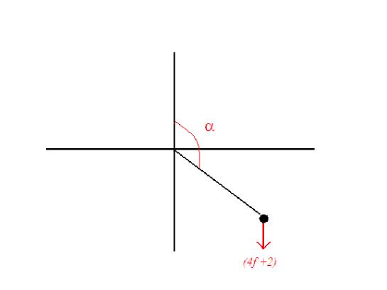
Figure 2:

The presence of the function $f(r)$ in eq.$\left(\ref{eq45}\right)$ is needed to ensure that expression $\left(\ref{eq45}\right)$ is a regular configuration. More precisely, we shall require that $A_{i}$ is regular at the origin, $r=0$, and that it goes to zero at infinity, $r=\infty$. Essentially, we shall consider two types of boundary conditions, namely the so called weak $\left(WBC\right)$ and strong $\left(SBC\right)$ boundary conditions [4, 5].

• For the $WBC$ we have

  $$A_{i} \;{is\;regular\;at\;the\;origin,}\;\;\;\;\;f(r)_{r\rightarrow 0}\rightarrow O(r)\;,$$

  $$A_{i} \;{decays\;as\;1/r\;for\;r\rightarrow\infty},\;\;\;\;f(r)_{r\rightarrow\infty}\rightarrow{constant}\;.$$

• For the $SBC$

  $$A_{i} \;{is\;regular\;at\;the\;origin,}\;\;\;\;\;f(r)_{r\rightarrow 0}\rightarrow O(r)\;,$$ (51)

  $$A_{i} \;decays\;faster\;than\;1/r\;for\;r\rightarrow\infty,\;\;\;\;\;f(r)_{r\rightarrow\infty}\rightarrow 0\;,$$

  $$(rA_{i})_{r\rightarrow\infty} \rightarrow 0\;.$$

Let us begin with the case of $SBC$. Recalling that $\partial\widehat{n}/\partial x_{i}\sim 1/r$ as $r\rightarrow\infty$, it follows that the equivalent field $\widetilde{A}_{i}$ in eq.$\left(\ref{eq46}\right)$ will obey $SBC$ if

$$\alpha(r) \rightarrow 2\pi m+\gamma r\;\;\;\;{for\;\;}{r\rightarrow 0\;,\;\;\;\;\;}m{\;\;{integer}}$$ (52)

$$\alpha(\tau) \rightarrow 2\pi m+\gamma e^{\tau}\;\;{for}\;\;{\tau\rightarrow-\infty\;,}$$

and

$$\alpha(r) \rightarrow 2\pi n\;\;\;{for}\;\;{r\rightarrow\infty}\;,\;\;\;\;n\;{{integer}}\;\;$$ (53)

$$\alpha(\tau) \rightarrow 2\pi n\;\;\;{for}\;\;{\tau\rightarrow\infty\;.}$$

Two situations are possible, according to the strength and the orientation of the force $f$.

• $i)\;$The first case corresponds to $\left(1+2f\;\right)>0$, see Fig.3.

  

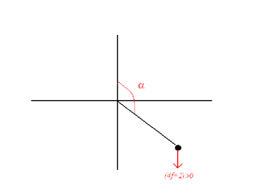
  Figure 3:

  At $\tau\rightarrow-\infty$, the pendulum starts at a position of unstable equilibrium, $\alpha=2\pi m$, with velocity $\alpha^{\prime}\sim\gamma e^{\tau}$, $\gamma\neq 0$, see Fig.4.

  

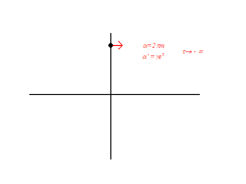
  Figure 4:

  For $\tau\rightarrow\infty$, after a certain number of oscillations, the pendulum falls down in the stable equilibrium point, see Fig.5, corresponding to $\alpha=(2p+1)\pi$, $p\;$integer, due to the force $\left(1+2f\;\right)$ and to the damping term. This situation does not correspond to $SBC$, since $\alpha=(2p+1)\pi$ for $\tau\rightarrow\infty$. Rather, it gives a copy $\widetilde{A}_{i}$ obeying $WBC$. Indeed, from eq.$\left(\ref{eq46}\right)$ we get

  $$\widetilde{A}_{r\rightarrow\infty}\sim\left(const.+\frac{(\cos(2p+1)\pi)-1}{2}\right)\frac{1}{r}\sim\frac{1}{r}\;.$$ (54)

  

  Figure 5:

• $ii)$ The second case corresponds to a force $f$ which, for a sufficiently large interval of time $\tau$, is negative enough, i.e., $f<-1/2$, see Fig.6. In this case we have the following configuration, see Fig.7. The pendulum starts at $\tau\rightarrow-\infty$ from an unstable position, $\alpha=2\pi m$, with velocity $\alpha^{\prime}\sim\gamma e^{\tau}$. After some oscillations, it can come back to the unstable position, $2\pi n$, at $\tau\rightarrow\infty$, under the effect of the force $f$, and finally it can remain there, see Fig.8. This situation corresponds to $SBC$, implying that the field $\widetilde{A}_{i}$ decays faster than $1/r$.

  

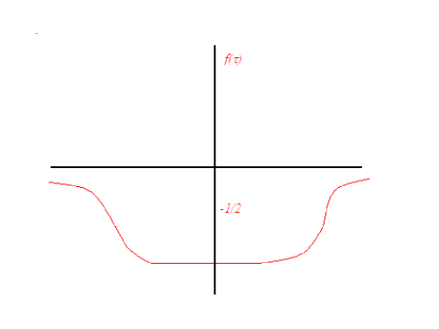
  Figure 6:

  

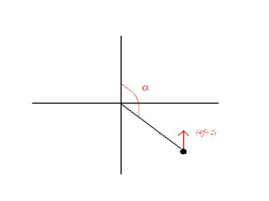
  Figure 7:

  

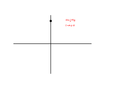
  Figure 8:

• Summary

  This example shows that, starting from the configuration

  $$A_{i}=\frac{i}{r^{2}}\varepsilon_{ijk}x_{j}\sigma_{k}f(r)\;,\;\;\;\;\partial_{i}A_{i}=0\;,\;\;$$ (55)

  we can obtain an equivalent field

  $$\widetilde{A}_{i}={S}^{\dagger}\partial_{i}{S}+S^{\dagger}A_{i}{S\;,\;\;\;}\partial_{i}\widetilde{A}_{i}=0\;,$$ (56)

  compatible with both $WBC$ and $\;SBC.\;$

  In the case of $SBC$

  $$\alpha(r)_{r\rightarrow\infty} \rightarrow 2\pi n\;,\;\;\;\;S_{r\rightarrow\infty}\rightarrow\;const.$$ (57)

  $$\left(r\widetilde{A}\right)_{r\rightarrow\infty} \rightarrow 0\;.$$

  For $WBC$

  $$\alpha(r)_{r\rightarrow\infty} \rightarrow\left(2p+1\right)\pi\;,\;\;\;\;$$ (58)

  $$S_{r\rightarrow\infty} \rightarrow\;\overrightarrow{\sigma}\cdot\overrightarrow{n}\;,\;S\;{depends\;on\;the\;orientation},\;S_{r\rightarrow\infty}\rightarrow S(\theta,\varphi)$$

  $$\widetilde{A}_{r\rightarrow\infty} \sim\frac{1}{r}\;.$$

2.2.1 The winding number of the Gribov copies

Let us evaluate now the winding number, see Appendix C, of the gauge transformation $S$

$$S=e^{\frac{i}{2}\alpha(r)\overrightarrow{n}\cdot\overrightarrow{\sigma}}=\cos\frac{\alpha}{2}+i\overrightarrow{n}\cdot\overrightarrow{\sigma}\sin\frac{\alpha}{2}\;.$$ (59)

We shall discuss in detail the case of $SBC$, namely

$$\alpha(r)_{r\rightarrow\infty}\rightarrow 2\pi n\;,$$ (60)

so that

$$S_{r\rightarrow\infty}\rightarrow\;const.$$ (61)

Equation $\left(\ref{w3}\right)$ implies that the space $\;R^{3}$ turns out to be compactified to the sphere $S^{3}$, by identifying all points at infinity. We have to evaluate

$$\nu=\frac{1}{24\pi^{2}}Tr\int dx_{1}dx_{2}dx_{3}\varepsilon_{ijk}\left(S^{\dagger}\partial_{i}S\right)\left(S^{\dagger}\partial_{j}S\right)\left(S^{\dagger}\partial_{k}S\right)\;.$$ (62)

From

$$S^{\dagger}\partial_{i}S=-\left(\partial_{i}S^{\dagger}\right)S\;,$$ (63)

we get

$$\nu=-\frac{1}{24\pi^{2}}Tr\int d^{3}x\varepsilon_{ijk}\left(\partial_{i}S\right)\left(S^{\dagger}\partial_{j}S\right)\left(\partial_{k}S^{\dagger}\right)\;.$$ (64)

It is useful to employ the notation

$$S = N_{4}+i\overrightarrow{N}\cdot\overrightarrow{\sigma}\;,\;\;\;\;\;\;S^{\dagger}=N_{4}-i\overrightarrow{N}\cdot\overrightarrow{\sigma}\;,$$

$$N_{4} = \cos\frac{\alpha}{2}\;,\;\;\;\;N_{i}=n_{i}\sin\frac{\alpha}{2}\;,\;\;\;\;$$ (65)

$$N_{a}N_{a} = 1\;,\;\;\;\;a=1,2,3,4\;.$$

In what follows we shall take in due account the surface terms originating from integration by parts. Thus

$$\nu = -\frac{1}{24\pi^{2}}Tr\int d^{3}x\varepsilon_{ijk}\left(\partial_{i}N_{4}+i\left(\partial_{i}\overrightarrow{N}\cdot\overrightarrow{\sigma}\right)\right)\left(N_{4}-i\overrightarrow{N}\cdot\overrightarrow{\sigma}\right)$$ (66)

$$\times\left(\partial_{j}N_{4}+i\left(\overrightarrow{\partial_{j}N}\cdot\overrightarrow{\sigma}\right)\right)\left(\partial_{k}N_{4}-i\left(\partial_{k}\overrightarrow{N}\cdot\overrightarrow{\sigma}\right)\right)\;$$

$$= -\frac{1}{24\pi^{2}}Tr\int d^{3}x\varepsilon_{ijk}\left[\left(\partial_{i}N_{4}\left(N_{4}-i\overrightarrow{N}\cdot\overrightarrow{\sigma}\right)+\left(\partial_{i}\overrightarrow{N}\cdot\overrightarrow{\sigma}\right)\left(iN_{4}+\overrightarrow{N}\cdot\overrightarrow{\sigma}\right)\right)\;\right.$$

$$\times\left.\left(\partial_{j}N_{4}\left(\partial_{k}N_{4}-i\partial_{k}\overrightarrow{N}\cdot\overrightarrow{\sigma}\right)+\left(\partial_{j}\overrightarrow{N}\cdot\overrightarrow{\sigma}\right)\left(i\partial_{k}N_{4}+\partial_{k}\overrightarrow{N}\cdot\overrightarrow{\sigma}\right)\right)\right]\;.$$

Since

$$\varepsilon_{ijk}\partial_{j}N_{4}\partial_{k}N_{4}=0\;,$$ (67)

we have

$$\nu = -\frac{Tr}{24\pi^{2}}\int d^{3}x\varepsilon_{ijk}\left[\partial_{i}N_{4}\left(\left(N_{4}-i\overrightarrow{N}\cdot\overrightarrow{\sigma}\right)\left(\partial_{j}\overrightarrow{N}\cdot\overrightarrow{\sigma}\right)\left(\partial_{k}\overrightarrow{N}\cdot\overrightarrow{\sigma}\right)\right)\right.$$

$$+N_{4}\left(\partial_{i}\overrightarrow{N}\cdot\overrightarrow{\sigma}\right)\left(\left(\partial_{j}N_{4}\right)\left(\partial_{k}\overrightarrow{N}\cdot\overrightarrow{\sigma}\right)-\left(\partial_{k}N_{4}\right)\left(\partial_{j}\overrightarrow{N}\cdot\overrightarrow{\sigma}\right)\right)$$

$$+\left(\partial_{i}\overrightarrow{N}\cdot\overrightarrow{\sigma}\right)\left(iN_{4}\left(\partial_{j}\overrightarrow{N}\cdot\overrightarrow{\sigma}\right)\left(\partial_{k}\overrightarrow{N}\cdot\overrightarrow{\sigma}\right)-i\left(\partial_{j}N_{4}\right)\left(\overrightarrow{N}\cdot\overrightarrow{\sigma}\right)\left(\partial_{k}\overrightarrow{N}\cdot\overrightarrow{\sigma}\right)\right)$$

$$\left.+\left(\partial_{i}\overrightarrow{N}\cdot\overrightarrow{\sigma}\right)\left(\overrightarrow{N}\cdot\overrightarrow{\sigma}\right)\left(\partial_{j}\overrightarrow{N}\cdot\overrightarrow{\sigma}\right)\left(i\partial_{k}N_{4}+\partial_{k}\overrightarrow{N}\cdot\overrightarrow{\sigma}\right)\right]\;.$$

From

$$\sigma_{i}\sigma_{j}=\delta_{ij}+i\varepsilon_{ijk}\sigma_{k}\;,$$ (69)

we find

$$Tr\sigma_{i}\sigma_{j} = 2\delta_{ij}\;,$$ (70)

$$Tr\left(\sigma_{i}\sigma_{j}\sigma_{k}\right) = 2i\varepsilon_{ijk}\;,$$

$$Tr\left(\sigma_{i}\sigma_{j}\sigma_{k}\sigma_{p}\right) = 2\left(\delta_{ij}\delta_{kp}-\delta_{ik}\delta_{jp}+\delta_{ip}\delta_{jk}\right)\;.$$

Furthermore, observing that

$$Tr\varepsilon_{ijk}\left(\partial_{i}N_{m}\right)N_{p}\left(\partial_{j}N_{q}\right)\left(\partial_{k}N_{r}\right)\sigma_{m}\sigma_{p}\sigma_{q}\sigma_{r}$$ (71)

$$= 2\varepsilon_{ijk}\left(\partial_{i}N_{m}\right)N_{p}\left(\partial_{j}N_{q}\right)\left(\partial_{k}N_{r}\right)\left(\delta_{mp}\delta_{qr}-\delta_{mq}\delta_{pr}+\delta_{mr}\delta_{pq}\right)$$

$$= 2\varepsilon_{ijk}\left[\left(\partial_{i}N_{m}\right)N_{m}\left(\partial_{j}N_{q}\right)\left(\partial_{k}N_{q}\right)-\left(\partial_{i}N_{m}\right)N_{p}\left(\partial_{j}N_{m}\right)\left(\partial_{k}N_{p}\right)\right]$$

$$+2\varepsilon_{ijk}\left(\partial_{i}N_{m}\right)N_{p}\left(\partial_{j}N_{p}\right)\left(\partial_{k}N_{m}\right)$$

$$= 0\;,$$

it follows

$$\nu=\frac{1}{24\pi^{2}}\int d^{3}x\varepsilon_{ijk}\varepsilon_{mpq}\left[2N_{4}\left(\partial_{i}N_{m}\right)\left(\partial_{j}N_{p}\right)\left(\partial_{k}N_{q}\right)-6\left(\partial_{i}N_{4}\right)N_{m}\left(\partial_{j}N_{p}\right)\left(\partial_{k}N_{q}\right)\right]\;.$$ (72)

Integrating by parts the second term, one obtains

$$\nu = \frac{1}{3\pi^{2}}\int d^{3}x\varepsilon_{ijk}\varepsilon_{mpq}N_{4}\left(\partial_{i}N_{m}\right)\left(\partial_{j}N_{p}\right)\left(\partial_{k}N_{q}\right)$$ (73)

$$-\frac{1}{4\pi^{2}}\int d^{3}x\varepsilon_{ijk}\partial_{i}\left(\varepsilon_{mpq}N_{4}N_{m}\left(\partial_{j}N_{p}\right)\left(\partial_{k}N_{q}\right)\right)\;.$$

Concerning the surface term in eq.$\left(\mathrm{{\ref{w14}}}\right)$, it turns out that

$$\varepsilon_{ijk}\varepsilon_{mpq}N_{4}N_{m}\left(\partial_{j}N_{p}\right)\left(\partial_{k}N_{q}\right)$$ (74)

$$= \cos\frac{\alpha}{2}\sin\frac{\alpha}{2}n_{m}\left(\partial_{j}\left(n_{p}\sin\frac{\alpha}{2}\right)\right)\left(\partial_{k}\left(n_{q}\sin\frac{\alpha}{2}\right)\right)\varepsilon_{ijk}\varepsilon_{mpq}$$

$$= \cos\frac{\alpha}{2}\sin^{3}\frac{\alpha}{2}n_{m}\left(\partial_{j}n_{p}\right)\left(\partial_{k}n_{q}\right)\varepsilon_{ijk}\varepsilon_{mpq}$$

$$= \frac{1}{r^{2}}\cos\frac{\alpha}{2}\sin^{3}\frac{\alpha}{2}n_{m}\left(\delta_{jp}-n_{j}n_{p}\right)\left(\delta_{kq}-n_{k}n_{q}\right)\varepsilon_{ijk}\varepsilon_{mpq}$$

$$= \frac{1}{r^{2}}\cos\frac{\alpha}{2}\sin^{3}\frac{\alpha}{2}n_{m}\varepsilon_{ijk}\varepsilon_{mjk}=\frac{2}{r^{2}}\cos\frac{\alpha}{2}\sin^{3}\frac{\alpha}{2}n_{i}\;.$$

Thus

$$\int d^{3}x\varepsilon_{ijk}\partial_{i}\left(\varepsilon_{mpq}N_{4}N_{m}\left(\partial_{j}N_{p}\right)\left(\partial_{k}N_{q}\right)\right)=\int d^{3}x\partial_{i}\left(\frac{2}{r^{2}}\cos\frac{\alpha}{2}\sin^{3}\frac{\alpha}{2}n_{i}\right)\;.$$ (75)

Moreover, recalling that $\alpha(r)_{r\rightarrow\infty}\rightarrow 2\pi n$, it follows that the surface term $\left(\ref{w16}\right)$ vanishes.

• Remark

  It is worth noticing that the surface term $\left(\ref{w16}\right)$ also vanishes in the case of $WBC$, due to the presence of $\cos\frac{\alpha}{2}$. Indeed, for $WBC$, $\alpha(r)_{r\rightarrow\infty}\rightarrow\left(2p+1\right)\pi$, so that $\cos\frac{\alpha(\infty)}{2}=\cos(p\pi+\frac{\pi}{2})=0.\;$Thus, for both $SBC$ and $WBC$, we have

  $$\nu=\frac{1}{3\pi^{2}}\int d^{3}x\varepsilon_{ijk}\varepsilon_{mpq}N_{4}\left(\partial_{i}N_{m}\right)\left(\partial_{j}N_{p}\right)\left(\partial_{k}N_{q}\right)\;.$$ (76)

Let us proceed then with the evaluation of expression $\left(\ref{w18}\right)$. We have

$$\nu = \frac{1}{3\pi^{2}}\int d^{3}x\varepsilon_{ijk}\varepsilon_{mpq}\cos\frac{\alpha}{2}\left(\partial_{i}\left(n_{m}\sin\frac{\alpha}{2}\right)\right)\left(\partial_{j}\left(n_{p}\sin\frac{\alpha}{2}\right)\right)\left(\partial_{k}\left(n_{q}\sin\frac{\alpha}{2}\right)\right)$$

$$= \frac{1}{3\pi^{2}}\int d^{3}x\varepsilon_{ijk}\varepsilon_{mpq}\cos\frac{\alpha}{2}\left[\left(\sin\frac{\alpha}{2}\left(\partial_{i}n_{m}\right)+\frac{n_{m}}{2}\cos\frac{\alpha}{2}\left(\partial_{i}\alpha\right)\right)\right.$$

$$\left.\times\left(\sin\frac{\alpha}{2}\left(\partial_{j}n_{p}\right)+\frac{n_{p}}{2}\cos\frac{\alpha}{2}\left(\partial_{j}\alpha\right)\right)\left(\sin\frac{\alpha}{2}\left(\partial_{k}n_{q}\right)+\frac{n_{q}}{2}\cos\frac{\alpha}{2}\left(\partial_{k}\alpha\right)\right)\right]\;$$

$$= \frac{1}{3\pi^{2}}\int d^{3}x\varepsilon_{ijk}\varepsilon_{mpq}\cos\frac{\alpha}{2}\left[\left(\sin^{2}\frac{\alpha}{2}\left(\partial_{i}n_{m}\right)\left(\partial_{j}n_{p}\right)+\frac{n_{p}}{2}\sin\frac{\alpha}{2}\cos\frac{\alpha}{2}\left(\partial_{i}n_{m}\right)\left(\partial_{j}\alpha\right)\right.\right.$$

$$\left.\left.+\frac{n_{m}}{2}\sin\frac{\alpha}{2}\cos\frac{\alpha}{2}\left(\partial_{i}\alpha\right)\left(\partial_{j}n_{p}\right)\right)\times\left(\sin\frac{\alpha}{2}\left(\partial_{k}n_{q}\right)+\frac{n_{q}}{2}\cos\frac{\alpha}{2}\left(\partial_{k}\alpha\right)\right)\right]\;$$

$$= \frac{1}{3\pi^{2}}\int d^{3}x\varepsilon_{ijk}\varepsilon_{mpq}\cos\frac{\alpha}{2}\left(\sin^{3}\frac{\alpha}{2}\left(\partial_{i}n_{m}\right)\left(\partial_{j}n_{p}\right)\left(\partial_{k}n_{q}\right)\right.$$

$$\;\;\;\;\;\;\;\;\;\;+\sin^{2}\frac{\alpha}{2}\cos\frac{\alpha}{2}\frac{n_{q}}{2}\left(\partial_{i}n_{m}\right)\left(\partial_{j}n_{p}\right)\left(\partial_{k}\alpha\right)$$

$$\;\;\;\;\;\;\;\;\;\;+\frac{n_{p}}{2}\sin^{2}\frac{\alpha}{2}\cos\frac{\alpha}{2}\left(\partial_{i}n_{m}\right)\left(\partial_{j}\alpha\right)\left(\partial_{k}n_{q}\right)$$

$$\;\;\;\;\;\;\;\;\;\;\left.+\frac{n_{m}}{2}\sin^{2}\frac{\alpha}{2}\cos\frac{\alpha}{2}\left(\partial_{i}\alpha\right)\left(\partial_{j}n_{p}\right)\left(\partial_{k}n_{q}\right)\right)$$

$$= \frac{1}{3\pi^{2}}\int d^{3}x\varepsilon_{ijk}\varepsilon_{mpq}\cos\frac{\alpha}{2}\left(\sin^{3}\frac{\alpha}{2}\left(\partial_{i}n_{m}\right)\left(\partial_{j}n_{p}\right)\left(\partial_{k}n_{q}\right)\;\right.$$

$$\left.+\frac{3}{2}\sin^{2}\frac{\alpha}{2}\cos\frac{\alpha}{2}n_{q}\left(\partial_{i}n_{m}\right)\left(\partial_{j}n_{p}\right)\left(\partial_{k}\alpha\right)\right)$$

Furthermore

$$\nu = \frac{1}{3\pi^{2}}\int d^{3}x\frac{1}{r^{3}}\cos\frac{\alpha}{2}\sin^{3}\frac{\alpha}{2}\varepsilon_{ijk}\varepsilon_{mpq}\left(\delta_{im}-n_{i}n_{m}\right)\left(\delta_{jp}-n_{j}n_{p}\right)\left(\delta_{kq}-n_{k}n_{q}\right)$$ (78)

$$+\frac{1}{2\pi^{2}}\int d^{3}x\sin^{2}\frac{\alpha}{2}\cos^{2}\frac{\alpha}{2}\alpha^{\prime}\frac{1}{r^{2}}\varepsilon_{ijk}\varepsilon_{mpq}n_{q}n_{k}\left(\delta_{im}-n_{i}n_{m}\right)\left(\delta_{jp}-n_{j}n_{p}\right)\;$$

$$= \frac{1}{3\pi^{2}}\int d^{3}x\frac{1}{r^{3}}\cos\frac{\alpha}{2}\sin^{3}\frac{\alpha}{2}\varepsilon_{ijk}\varepsilon_{mpq}\left(\left(\delta_{im}\delta_{jp}-\delta_{im}n_{j}n_{p}-\delta_{jp}n_{i}n_{m}\right)\left(\delta_{kq}-n_{k}n_{q}\right)\right)$$

$$+\frac{1}{2\pi^{2}}\int d^{3}x\sin^{2}\frac{\alpha}{2}\cos^{2}\frac{\alpha}{2}\alpha^{\prime}\frac{1}{r^{2}}\varepsilon_{ijk}\varepsilon_{mpq}n_{q}n_{k}\left(\delta_{im}\delta_{jp}-\delta_{im}n_{j}n_{p}-\delta_{jp}n_{i}n_{m}\right)$$

$$= \frac{1}{3\pi^{2}}\int d^{3}x\frac{1}{r^{3}}\cos\frac{\alpha}{2}\sin^{3}\frac{\alpha}{2}\varepsilon_{ijk}\varepsilon_{mpq}\left(\delta_{im}\left(\delta_{jp}\delta_{kq}-\delta_{jp}n_{k}n_{q}-\delta_{kq}n_{j}n_{p}\right)-\delta_{jp}\delta_{kq}n_{i}n_{m}\right)$$

$$+\frac{1}{2\pi^{2}}\int d^{3}x\sin^{2}\frac{\alpha}{2}\cos^{2}\frac{\alpha}{2}\alpha^{\prime}\frac{1}{r^{2}}\varepsilon_{ijk}\varepsilon_{mpq}n_{q}n_{k}\delta_{im}\delta_{jp}$$

$$= \frac{1}{3\pi^{2}}\int d^{3}x\frac{1}{r^{3}}\cos\frac{\alpha}{2}\sin^{3}\frac{\alpha}{2}\varepsilon_{ijk}\varepsilon_{mpq}\left(\delta_{im}\delta_{jp}\delta_{kq}-3\delta_{im}\delta_{jp}n_{k}nq\right)$$

$$+\frac{1}{2\pi^{2}}\int d^{3}x\sin^{2}\frac{\alpha}{2}\cos^{2}\frac{\alpha}{2}\alpha^{\prime}\frac{1}{r^{2}}\varepsilon_{ijk}\varepsilon_{ijq}n_{q}n_{k}$$

$$= \frac{1}{3\pi^{2}}\int d^{3}x\frac{1}{r^{3}}\cos\frac{\alpha}{2}\sin^{3}\frac{\alpha}{2}\left(\varepsilon_{ijk}\varepsilon_{ijk}-3\varepsilon_{ijk}\varepsilon_{ijq}n_{k}nq\right)$$

$$+\frac{1}{\pi^{2}}\int d^{3}x\sin^{2}\frac{\alpha}{2}\cos^{2}\frac{\alpha}{2}\alpha^{\prime}\frac{1}{r^{2}}$$

$$= \frac{1}{\pi^{2}}\int d^{3}x\sin^{2}\frac{\alpha}{2}\cos^{2}\frac{\alpha}{2}\alpha^{\prime}\frac{1}{r^{2}}$$

In order to evaluate this last integral we shall make use of polar coordinates

$$\nu = \frac{4}{\pi}\int_{0}^{\infty}dr\sin^{2}\frac{\alpha}{2}\cos^{2}\frac{\alpha}{2}\alpha^{\prime}=-\frac{1}{4\pi}\int_{0}^{\infty}dr\alpha^{\prime}\left(e^{i\frac{\alpha}{2}}+e^{-i\frac{\alpha}{2}}\right)^{2}\left(e^{i\frac{\alpha}{2}}-e^{-i\frac{\alpha}{2}}\right)^{2}$$ (79)

$$= -\frac{1}{4\pi}\int_{0}^{\infty}dr\alpha^{\prime}\left(e^{i\alpha}+e^{-i\alpha}+2\right)\left(e^{i\alpha}+e^{-i\alpha}-2\right)$$

$$= \frac{1}{2\pi}\int_{0}^{\infty}dr\alpha^{\prime}\left(1-\cos 2\alpha\right)\;.$$

Finally, for the winding number $\nu$ associated to the gauge transformation $S$, we find

$$\nu=\frac{1}{2\pi}\left(\alpha(\infty)-\alpha(0)\right)-\frac{1}{4\pi}\left(\sin 2\alpha(\infty)-\sin 2\alpha(0)\right)\;.$$ (80)

• Summary

  Let us consider first the case of $SBC.$ From

  $$\alpha(r)_{r\rightarrow\infty} \rightarrow 2\pi n\;,\;\;\;n\;\;\;\;{integer}\;$$

  $$\alpha(r)_{r\rightarrow 0} \rightarrow 2\pi m\;,\;\;\;m\;\;{integer}\;,$$ (81)

  it follows

  $$\nu_{SBC}=\;\;{{integer}}$$ (82)

  For $WBC$

  $$\alpha(r)_{r\rightarrow\infty} \rightarrow \left(2p+1\right)\pi\;,\;\;\;\;p\;\;{integer}\;$$

  $$\alpha(r)_{r\rightarrow 0} \rightarrow 2\pi m\;,\;\;\;\;\;\;\;\;\;\;m\;\;{\;}{integer}{\;},$$ (83)

  we have

  $$\nu_{WBC}=\;\left({integer}+\frac{1}{2}\right)\;.$$ (84)

• Remark

  It should be noted that, in the case of WBC, the expression $\left(\ref{w4}\right)$ does not have the meaning of a winding number. In fact, due to the behavior of the gauge transformation $S$ at infinity, eq.$\left(\ref{eq57}\right)$, the space $\;R^{3}$ cannot be compactified to the sphere $S^{3}$. As a consequence, expression $\left(\ref{w4}\right)$ may now take non integer values.

2.2.2 The Gribov copies of the vacuum

Let us discuss now the existence of the Gribov copies of the vacuum, $A_{i}=0$, which obviously satisfies $\partial_{i}A_{i}=0$. We look at the equivalent field

$$\widetilde{A}_{i} = {S}^{\dagger}\partial_{i}{S\;=}\frac{1}{2}\sin\alpha\frac{\partial\widehat{n}}{\partial x_{i}}+\left(\frac{1}{2}\cos\alpha-\frac{1}{2}\right)\widehat{n}\frac{\partial\widehat{n}}{\partial x_{i}}+\frac{1}{2}\alpha^{\prime}(r)\widehat{n}n_{i}\;,$$

$$S = e^{\frac{i}{2}\alpha(r)\overrightarrow{n}\cdot\overrightarrow{\sigma}}=\cos\frac{\alpha}{2}+i\overrightarrow{n}\cdot\overrightarrow{\sigma}\sin\frac{\alpha}{2}\;,$$ (85)

which corresponds to a pure gauge

$$\widetilde{A}_{i}=S^{\dagger}\partial_{i}S\;,\;\;\;\;F_{ij}(\widetilde{A})=0\;.$$

The gauge condition $\partial_{i}\widetilde{A}_{i}=0$ reads now

$$\alpha^{\prime\prime}(r)+\frac{2}{r}\alpha^{\prime}(r)-\frac{2}{r^{2}}\sin\alpha=0\;,$$ (86)

or, $\tau=\log r$,

$$\frac{\partial^{2}\alpha(\tau)}{\partial\tau^{2}}+\frac{\partial\alpha(\tau)}{\partial\tau}-2\sin\alpha=0\;,$$ (87)

corresponding to the damped pendulum of Fig.9.

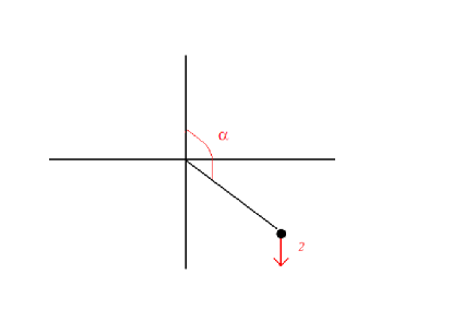
Figure 9:

The regularity condition of the equivalent field $\widetilde{A}_{i}$ at the origin, $r=0$, $\tau=-\infty$, gives

$$\alpha(r) \rightarrow 2\pi m+\gamma r\;\;{for\;}{\ r\rightarrow 0}\;,\;\;\;\;\;m\;\;{{integer}}$$ (88)

$$\alpha(\tau) \rightarrow 2\pi m+\gamma e^{\tau}\;{for}\;{\tau\rightarrow-\infty\;,}$$

which holds for both $WBC$ and $SBC$. Since the force $f$ is now absent, the pendulum starts at $\tau\rightarrow-\infty$ from the unstable position, $\alpha=2\pi m$, with velocity $\alpha^{\prime}=\gamma e^{\tau}$, see Fig.10.

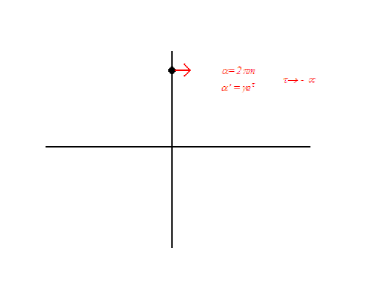
Figure 10:

After a certain number of oscillations it comes to the stable position $\alpha_{\tau\rightarrow\infty}=\left(2p+1\right)\pi$, due to the constant force and to the damping, see Fig.11.

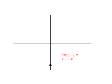
Figure 11:

Thus, in the absence of the force $f$, there are no Gribov copies of the vacuum if $SBC$ are imposed. However, if $WBC$ are adopted, even the vacuum has Gribov copies. As we have already seen, this corresponds to an equivalent field $\widetilde{A}_{i}$ which, for $\alpha_{\tau\rightarrow\infty}=\left(2p+1\right)\pi$, behaves as

$$\widetilde{A}_{r\rightarrow\infty}\sim\left(\cos(2p+1)\pi-1\right)\frac{1}{r}\sim\frac{1}{r}\;.$$ (89)

2.3 The Henyey example

In this section we shall discuss a class of Gribov’s copies proposed by Henyey [2]. The relevance of Henyey’s work is due to the fact that Gribov’s copies with vanishing winding number and which fall off faster than $1/r$, for $r\rightarrow\infty$, are explicitly obtained.

The starting configuration is

$$\overrightarrow{A}=i\overrightarrow{a}\sigma_{3}\;,\;\;\;\partial_{i}A_{i}=0\;.$$ (90)

Notice that the gauge configuration, eq.$\left(\ref{h1}\right)$, lies in the abelian diagonal subgroup of $SU(2)$. We shall consider the set of gauge transformations parametrized by

$$S=e^{i\alpha\overrightarrow{f}\cdot\overrightarrow{\sigma}}=\cos\alpha+i\overrightarrow{f}\cdot\overrightarrow{\sigma}\sin\alpha\;,$$ (91)

where $\overrightarrow{f}$ is the unit vector

$$\overrightarrow{f}\cdot\overrightarrow{f} = 1\;,$$ (92)

$$\overrightarrow{f} = \overrightarrow{e}_{x}\cos\beta+\overrightarrow{e}_{y}\sin\beta\;,$$

and $\left(\overrightarrow{e}_{x},\overrightarrow{e}_{y},\overrightarrow{e}_{z}\right)$ are the unit orthogonal cartesian vectors. Introducing the vector $\overrightarrow{g}$

$$\overrightarrow{g}=-\overrightarrow{e}_{x}\sin\beta+\overrightarrow{e}_{y}\cos\beta\;,$$ (93)

it turns out that the set $\left(\overrightarrow{f},\overrightarrow{g},\overrightarrow{e}_{z}\right)$ yields a right-handed orthonormal triad which rotates about the $z$-axis. Also,

$$\partial_{i}\overrightarrow{f}=\overrightarrow{g}\partial_{i}\beta\;,\;\;\;\;\;\partial_{i}\overrightarrow{g}=-\overrightarrow{f}\partial_{i}\beta\;.$$ (94)

Let us evaluate the gauge transformed field $\widetilde{A}_{i}$

$$\widetilde{A}_{i} = {S}^{\dagger}\partial_{i}{S}+S^{\dagger}A_{i}{S}$$

$$= i\left(\cos\alpha-i\overrightarrow{f}\cdot\overrightarrow{\sigma}\sin\alpha\right)a_{i}\sigma_{3}\left(\cos\alpha+i\overrightarrow{f}\cdot\overrightarrow{\sigma}\sin\alpha\right)\;$$

$$+\left(\cos\alpha-i\overrightarrow{f}\cdot\overrightarrow{\sigma}\sin\alpha\right)\left(-\sin\alpha+i\overrightarrow{f}\cdot\overrightarrow{\sigma}\cos\alpha\right)\partial_{i}\alpha$$

$$+i\left(\cos\alpha-i\overrightarrow{f}\cdot\overrightarrow{\sigma}\sin\alpha\right)\overrightarrow{g}\cdot\overrightarrow{\sigma}\sin\alpha\partial_{i}\beta\;.$$

Recalling that $\left(\overrightarrow{f}\cdot\overrightarrow{\sigma}\right)^{2}=1$, it follows that

$$\widetilde{A}_{i} = ia_{i}\left(\cos^{2}\alpha\sigma_{3}+i\sin\alpha\cos\alpha f_{k}\left[\sigma_{3},\sigma_{k}\right]+\sin^{2}\alpha f_{k}f_{m}\sigma_{k}\sigma_{3}\sigma_{m}\right)$$

$$+i\partial_{i}\alpha\overrightarrow{f}\cdot\overrightarrow{\sigma}+\partial_{i}\beta\left(i\sin\alpha\cos\alpha\overrightarrow{g}\cdot\overrightarrow{\sigma}+\sin^{2}\alpha\left(\overrightarrow{f}\cdot\overrightarrow{\sigma}\right)\left(\overrightarrow{g}\cdot\overrightarrow{\sigma}\right)\right)\;$$

$$= ia_{i}\left(\cos^{2}\alpha\sigma_{3}-2\sin\alpha\cos\alpha\varepsilon_{3km}\sigma_{m}f_{k}+\sin^{2}\alpha f_{k}f_{m}\sigma_{k}\left(\delta_{3m}+i\varepsilon_{3mp}\sigma_{p}\right)\right)$$

$$+i\partial_{i}\alpha\overrightarrow{f}\cdot\overrightarrow{\sigma}+\partial_{i}\beta\left(i\sin\alpha\cos\alpha\overrightarrow{g}\cdot\overrightarrow{\sigma}+\sin^{2}\alpha f_{i}g_{k}\left(\delta_{ik}+i\varepsilon_{ikm}\sigma_{m}\right)\right)\;.$$

From

$$\varepsilon_{3km}\sigma_{m}f_{k} = \left(\overrightarrow{e}_{z}\times\overrightarrow{f}\right)\cdot\overrightarrow{\sigma}=\left(\overrightarrow{e}_{z}\times\left(\overrightarrow{e}_{x}\cos\beta+\overrightarrow{e}_{y}\sin\beta\right)\right)\cdot\overrightarrow{\sigma}$$

$$= \left(\overrightarrow{e}_{y}\cos\beta-\overrightarrow{e}_{x}\sin\beta\right)\cdot\overrightarrow{\sigma}=\overrightarrow{g}\cdot\overrightarrow{\sigma}\;,$$

$$f_{i}g_{k}\varepsilon_{ikm}\sigma_{m} = \left(\overrightarrow{f}\times\overrightarrow{g}\right)\cdot\overrightarrow{\sigma}=\left(\left(\overrightarrow{e}_{x}\cos\beta+\overrightarrow{e}_{y}\sin\beta\right)\times\left(-\overrightarrow{e}_{x}\sin\beta+\overrightarrow{e}_{y}\cos\beta\right)\right)\cdot\overrightarrow{\sigma}\;$$

$$= \overrightarrow{e}_{z}\cdot\overrightarrow{\sigma}\;=\sigma_{3}\;,$$

$$f_{k}f_{m}\varepsilon_{3mp}\sigma_{k}\sigma_{p} = f_{k}f_{m}\varepsilon_{3mp}\left(\delta_{kp}+i\varepsilon_{kpq}\sigma_{q}\right)=f_{k}f_{m}\varepsilon_{3mk}-if_{k}f_{m}\varepsilon_{3mp}\varepsilon_{pkq}\sigma_{q}$$

$$= -if_{k}f_{m}\left(\delta_{3k}\delta_{mq}-\delta_{3q}\delta_{mk}\right)\sigma_{q}=i\sigma_{3\;,}$$

$$f_{3} = 0\;,\;\;\;\overrightarrow{f}\cdot\overrightarrow{g}=0\mathrm{{\ },\;}$$ (97)

it follows

$$\widetilde{A}_{i} = \;ia_{i}\left(\cos^{2}\alpha\sigma_{3}-2\sin\alpha\cos\alpha\overrightarrow{g}\cdot\overrightarrow{\sigma}-\sin^{2}\alpha\sigma_{3}\right)+i\partial_{i}\alpha\overrightarrow{f}\cdot\overrightarrow{\sigma}$$ (98)

$$+\partial_{i}\beta\left(i\sin\alpha\cos\alpha\overrightarrow{g}\cdot\overrightarrow{\sigma}+i\sin^{2}\alpha\sigma_{3}\right)\;.$$

Finally, from $\left(\cos^{2}\alpha-\sin^{2}\alpha\right)=\cos 2\alpha$, we get

$$\widetilde{A}_{i} = i\sigma_{3}\left(a_{i}\cos 2\alpha+\partial_{i}\beta\sin^{2}\alpha\right)+i\partial_{i}\alpha\overrightarrow{f}\cdot\overrightarrow{\sigma}$$ (99)

$$+i\overrightarrow{g}\cdot\overrightarrow{\sigma}\left(-a_{i}\sin 2\alpha+\frac{1}{2}\partial_{i}\beta\sin 2\alpha\right)\;.$$

Let us turn now to the condition $\partial_{i}\widetilde{A}_{i}=0$. Computing the divergence of $\widetilde{A}_{i}$, yields

$$\partial_{i}\widetilde{A}_{i} = i\sigma_{3}\left(-2a_{i}\partial_{i}\alpha\sin 2\alpha+\partial^{2}\beta\sin^{2}\alpha+2\sin\alpha\cos\alpha\partial_{i}\beta\partial_{i}\alpha\right)$$

$$+i\partial^{2}\alpha\overrightarrow{f}\cdot\overrightarrow{\sigma}+i\partial_{i}\alpha\partial_{i}\beta\overrightarrow{g}\cdot\overrightarrow{\sigma}\;$$

$$-i\partial_{i}\beta\overrightarrow{f}\cdot\overrightarrow{\sigma}\left(-a_{i}\sin 2\alpha+\frac{1}{2}\partial_{i}\beta\sin 2\alpha\right)$$

$$+i\overrightarrow{g}\cdot\overrightarrow{\sigma}\left(-2a_{i}\partial_{i}\alpha\cos 2\alpha+\frac{1}{2}\partial^{2}\beta\sin 2\alpha+\partial_{i}\beta\partial_{i}\alpha\cos 2\alpha\right)=0\;.$$

Following Henyey [2], we shall impose

$$\partial^{2}\beta=\partial_{i}\partial_{i}\beta=0\;,\;\;\;\;a_{i}\partial_{i}\alpha=0\;,\;\;\;\;\partial_{i}\beta\partial_{i}\alpha=0\;.$$ (101)

Thus, the condition $\partial_{i}\widetilde{A}_{i}=0$ reduces to

$$\partial^{2}\alpha+a_{i}\partial_{i}\beta\sin 2\alpha-\frac{1}{2}\partial_{i}\beta\partial_{i}\beta\sin 2\alpha=0\;.$$ (102)

• Summary

  $$\overrightarrow{A}=i\overrightarrow{a}\sigma_{3}\;,\;\;\;\partial_{i}A_{i}=\partial_{i}a_{i}=0\;.$$ (103)

  $$S = e^{i\alpha\overrightarrow{f}\cdot\overrightarrow{\sigma}}=\cos\alpha+i\overrightarrow{f}\cdot\overrightarrow{\sigma}\sin\alpha\;,$$

  $$\overrightarrow{f} = \overrightarrow{e}_{x}\cos\beta+\overrightarrow{e}_{y}\sin\beta\;,\;\;\;\;\overrightarrow{f}\cdot\overrightarrow{f}=1\;.$$ (104)

  For the gauge transformed field we get

  $$\widetilde{A}_{i} = {S}^{\dagger}\partial_{i}{S}+S^{\dagger}A_{i}{S}$$ (105)

  $$= i\sigma_{3}\left(a_{i}\cos 2\alpha+\partial_{i}\beta\sin^{2}\alpha\right)+i\partial_{i}\alpha\overrightarrow{f}\cdot\overrightarrow{\sigma}$$

  $$+i\overrightarrow{g}\cdot\overrightarrow{\sigma}\left(-a_{i}\sin 2\alpha+\frac{1}{2}\partial_{i}\beta\sin 2\alpha\right)\;.$$

  The condition for the existence of Gribov’s copies, $\partial_{i}\widetilde{A}_{i}=0$ gives

  $$\partial^{2}\beta=\partial_{i}\partial_{i}\beta=0\;,\;\;\;\;a_{i}\partial_{i}\alpha=0\;,\;\;\;\;\partial_{i}\beta\partial_{i}\alpha=0\;,\;$$ (106)

  and

  $$\partial^{2}\alpha+a_{i}\partial_{i}\beta\sin 2\alpha-\frac{1}{2}\partial_{i}\beta\partial_{i}\beta\sin 2\alpha=0\;.$$ (107)

2.3.1 Henyey’s solution

In order to solve the eqs.$\left(\ref{sh4}\right)$, $\left(\ref{sh5}\right)$ it is useful to adopt polar coordinates [2], see Appendix D. We set

$$\overrightarrow{a}=a(r,\theta)\overrightarrow{e}_{\varphi}\;,\;\;\;\;\beta=\beta(\varphi)\;,\;\;\;\;\alpha=\alpha(r,\theta)\;.$$ (108)

The equations

$$\overrightarrow{\nabla}\cdot\overrightarrow{a} = \frac{1}{r\sin\theta}\frac{\partial}{\partial\varphi}a(r,\theta)=0\;,$$ (109)

$$\overrightarrow{a}\cdot\overrightarrow{\nabla}\alpha = a(r,\theta)\frac{1}{r\sin\theta}\frac{\partial}{\partial\varphi}\alpha(r,\theta)=0\;,$$

$$\overrightarrow{\nabla}\alpha\cdot\overrightarrow{\nabla}\beta = 0\;,$$

are fulfilled. From

$$\overrightarrow{\nabla}^{2}\beta=\frac{1}{r^{2}\sin^{2}\theta}\frac{\partial^{2}}{\partial\varphi^{2}}\beta=0\;,$$ (110)

it follows that we may take

$$\beta=\varphi\;.$$ (111)

It remains to solve the condition $\left(\ref{sh5}\right)$, which now reads

$$\frac{1}{r^{2}}\frac{\partial}{\partial r}\left(r^{2}\frac{\partial\alpha}{\partial r}\right)+\frac{1}{r^{2}\sin\theta}\frac{\partial}{\partial\theta}\left(\sin\theta\frac{\partial\alpha}{\partial\theta}\right)+\sin 2\alpha\left(\frac{a}{r\sin\theta}-\frac{1}{2r^{2}\sin^{2}\theta}\right)=0\;.$$ (112)

Setting

$$\alpha(r,\theta)=rb(r)\sin\theta\;,$$ (113)

equation $\left(\ref{h18}\right)$ becomes

$$b+\left(r^{2}b^{\prime\prime}+4rb^{\prime}\right)\sin^{2}\theta+\left(a-\frac{1}{2r\sin\theta}\right)\sin\left(2rb\sin\theta\right)=0\;.$$ (114)

The strategy adopted by Henyey [2] in order to solve this equation is that of expressing $a$ in terms of $b$, and then searching for a suitable $b$ which gives the desired behavior for $a$. Accordingly, we write

$$a=\frac{1}{2r\sin\theta}-\frac{1}{\sin\left(2rb\sin\theta\right)}\left(b+r^{2}\sin^{2}\theta\left(b^{\prime\prime}+4\frac{b^{\prime}}{r}\right)\right)\;.$$ (115)

We look then for a function $b$ such that:

$$a\;{\ }{\ }{\ }\mathrm{is\;regular\;at\;the\;origin},\;\;r \rightarrow 0\;,$$ (116)

$$a\;{\ }{\ }{\ }\mathrm{decays\;faster\;than}\;1/r\;\mathrm{for}\;r \rightarrow \infty\;.$$

First of all we notice that expression $\left(\ref{h21}\right)$ is not singular at $\theta=0$. Although each term of eq.$\left(\ref{h21}\right)$ is singular, their sum has no singularity at $\theta=0$, i.e.

$$a_{\theta\rightarrow 0}\approx\frac{1}{2r\theta}-\frac{1}{2rb\theta}\left(b+r^{2}\theta^{2}\left(b^{\prime\prime}+4\frac{b^{\prime}}{r}\right)\right)=0\;.$$ (117)

Also, in order to avoid possible singularities in the term $\left(1/\sin\left(2rb\sin\theta\right)\right)$ we require

$$2rb(r)<\pi\;.$$ (118)

Since $\sin\theta\leq 1$, the condition $\left(\ref{h24}\right)$ implies that the argument of $\sin\left(2rb\sin\theta\right)$ cannot be equal to $\pi$, i.e. $2rb\sin\theta<\pi$.

Let us look now at $r=0$. We have

$$a_{r\rightarrow 0}\approx\frac{1}{2r\sin\theta}-\frac{1}{2rb\sin\theta}\left(b+r^{2}\sin^{2}\theta\left(b^{\prime\prime}+4\frac{b^{\prime}}{r}\right)\right)\;.$$ (119)

Requiring that

$$\left.b(r)\right._{r\rightarrow 0}\approx b_{0}+b_{2}r^{2}+O(r^{3})\;,\;\;\;\;\;\;\mathrm{with}\;\;b_{0}\neq 0\;,$$ (120)

it follows

$$a_{r\rightarrow 0}\approx\frac{1}{2r\sin\theta}-\frac{1}{2rb\sin\theta}+O(r)\approx O(r)\;,$$ (121)

so that $a$ is regular at the origin. It remains now to discuss the limit $r\rightarrow\infty$. In this case we search for a $b(r)$ such that $r^{2}a\rightarrow 0$ for $r\rightarrow\infty$. Let us set

$$\left.b(r)\right._{r\rightarrow\infty}\approx\frac{1}{r^{n}}\;,$$ (122)

and let us determine $n$. From

$$\left.r^{2}a\right._{r\rightarrow\infty} \approx r^{2}\left(\frac{1}{2r\sin\theta}-\frac{1}{r^{n}}\frac{1}{\sin\left(\frac{2\sin\theta}{r^{n-1}}\right)}\right)-\frac{r^{4}\sin^{2}\theta}{\sin\left(\frac{2\sin\theta}{r^{n-1}}\right)}\left(n(n+1)-4n)\right)\frac{1}{r^{n+2}}$$ (123)

$$\approx r^{2}\left(\frac{1}{2r\sin\theta}-\frac{1}{r^{n}}\frac{1}{\left(\frac{2\sin\theta}{r^{n-1}}\right)+O\left(\frac{1}{r^{3n-3}}\right)}\right)-n(n-3)\frac{r^{4}}{r^{n+2}}\frac{\sin^{2}\theta}{\sin\left(\frac{2\sin\theta}{r^{n-1}}\right)}$$

$$\approx O\left(\frac{1}{r^{2n-5}}\right)-n(n-3)\frac{r\sin\theta}{2}\;.$$

Thus, if $n=3$,

$$\left.b(r)\right._{r\rightarrow\infty} \approx \frac{1}{r^{3}}\;,$$ (124)

$$\left.r^{2}a(r)\right._{r\rightarrow\infty} \approx O\left(\frac{1}{r}\right)\;.$$

• Summary

  In summary, any function $b(r)$ such that

  $$\left.b(r)\right._{r\rightarrow 0} \approx b_{0}+b_{2}r^{2}+O(r^{3})\;,\;\;\;\;\;\;\mathrm{with}\;\;b_{0}\neq 0\;,$$

  $$2rb(r) < \pi\;,$$

  $$\left.b(r)\right._{r\rightarrow\infty} \approx \frac{1}{r^{3}}\;,$$ (125)

  will give a gauge field $\overrightarrow{A}$

  $$\overrightarrow{A} = i\overrightarrow{a}\sigma_{3}\;,\;\;\;\partial_{i}A_{i}=\partial_{i}a_{i}=0\;.$$ (126)

  $$\overrightarrow{a} = a(r,\theta)\overrightarrow{e}_{\varphi}$$

  $$a(r,\theta) = \frac{1}{2r\sin\theta}-\frac{1}{\sin\left(2rb\sin\theta\right)}\left(b+r^{2}\sin^{2}\theta\left(b^{\prime\prime}+4\frac{b^{\prime}}{r}\right)\right)$$

  which is regular at the origin, $r=0$, and decays faster than $1/r^{2}$ at infinity, $r\rightarrow\infty$

  $$a_{r\rightarrow 0} \approx O(r)\;,$$

  $$\left.r^{2}a(r)\right._{r\rightarrow\infty} \approx O\left(\frac{1}{r}\right)\;.$$ (127)

  An example of such a function $b(r)$ is given by

  $$b(r) = \frac{k}{\left(r^{2}+r_{0}^{2}\right)^{3/2}}\;,$$

  $$k < \frac{3^{3/2}\pi}{4}r_{0}^{2}\;,$$ (128)

  where the condition $k<\left(3^{3/2}\pi r_{0}^{2}\right)/4\;$stems from the requirement $2rb(r)<\pi.$

2.3.2 The winding number of Henyey’s solution

It remains now to discuss the winding number of Henyey’s solution. Let us begin with the evaluation of the winding number corresponding to the gauge transformation $\left(\ref{h2}\right)$

$$S=e^{i\alpha\overrightarrow{f}\cdot\overrightarrow{\sigma}}=\cos\alpha+i\overrightarrow{f}\cdot\overrightarrow{\sigma}\sin\alpha\;.$$ (129)

From expression $\left(\ref{w14}\right)$, we have

$$\nu = \frac{1}{3\pi^{2}}\int d^{3}x\varepsilon_{ijk}\varepsilon_{mpq}N_{4}\left(\partial_{i}N_{m}\right)\left(\partial_{j}N_{p}\right)\left(\partial_{k}N_{q}\right)$$ (130)

$$-\frac{1}{4\pi^{2}}\int d^{3}x\varepsilon_{ijk}\partial_{i}\left(\varepsilon_{mpq}N_{4}N_{m}\left(\partial_{j}N_{p}\right)\left(\partial_{k}N_{q}\right)\right)\;,$$

with

$$N_{4}=\cos\alpha\;,\;\;\;\;N_{i}=f_{i}\sin\alpha\;.$$ (131)

Recalling that

$$\partial_{i}\overrightarrow{f}=\overrightarrow{g}\partial_{i}\beta\;,\;\;\;\;\overrightarrow{f}\cdot\overrightarrow{g}=0\;,$$ (132)

it follows

$$\nu = \frac{1}{3\pi^{2}}\int d^{3}x\varepsilon_{ijk}\varepsilon_{mpq}\cos\alpha\left[\left(\sin\alpha g_{m}\partial_{i}\beta+f_{m}\cos\alpha\partial_{i}\alpha\right)\left(\sin\alpha g_{p}\partial_{j}\beta+f_{p}\cos\alpha\partial_{j}\alpha\right)\right.$$

$$\;\;\;\;\;\;\;\;\;\;\;\;\;\;\;\;\left.\;\times\left(\sin\alpha g_{q}\partial_{k}\beta+f_{q}\cos\alpha\partial_{k}\alpha\right)\right]$$

$$-\frac{1}{4\pi^{2}}\int d^{3}x\varepsilon_{ijk}\partial_{i}\left[\varepsilon_{mpq}\sin\alpha\cos\alpha f_{m}\left(\sin\alpha g_{p}\partial_{j}\beta+f_{p}\cos\alpha\partial_{j}\alpha\right)\right.$$

$$\;\;\;\;\;\;\;\;\;\;\;\;\;\;\;\;\left.\times\left(\sin\alpha g_{q}\partial_{k}\beta+f_{q}\cos\alpha\partial_{k}\alpha\right)\right]$$

$$= \frac{1}{3\pi^{2}}\int d^{3}x\varepsilon_{ijk}\varepsilon_{mpq}\cos\alpha\left[\left(\sin\alpha\cos\alpha g_{m}f_{p}\partial_{i}\beta\partial_{j}\alpha+\sin\alpha\cos\alpha f_{m}g_{p}\partial_{i}\alpha\partial_{j}\beta\right)\right.$$

$$\;\;\;\;\;\;\;\;\;\;\;\;\;\;\;\;\left.\times\left(\sin\alpha g_{q}\partial_{k}\beta+f_{q}\cos\alpha\partial_{k}\alpha\right)\right]$$

$$-\frac{1}{4\pi^{2}}\int d^{3}x\varepsilon_{ijk}\partial_{i}\left(\varepsilon_{mpq}\sin\alpha\cos\alpha f_{m}\left(\sin\alpha g_{p}\partial_{j}\beta\right)\left(\sin\alpha g_{q}\partial_{k}\beta\right)\right)$$

$$= 0\;.$$ (134)

We proceed now with the computation of the winding number of the starting gauge configuration $\left(\ref{h2}\right)$ and of the gauge copy $\left(\ref{h6}\right)$. To obtain the winding number of the expression $\left(\ref{h2}\right)$, we start from the Pontryagin index, eqs.$\left(\ref{c50}\right)-\left(\ref{c52}\right)\;$of Appendix C,

$$\nu\;=-\frac{1}{8\pi^{2}}Tr\int_{S_{\infty}^{3}}dS_{\mu}\varepsilon_{\mu\nu\rho\sigma}\left(A_{\nu}\partial_{\rho}A_{\sigma}+\frac{2}{3}A_{\nu}A_{\rho}A_{\sigma}\right)\;.$$ (135)

From

$$\overrightarrow{A}=i\overrightarrow{a}\sigma_{3}\;,\;\;\;\partial_{i}A_{i}=0\;,\;\;$$ (136)

and

$$A_{4}=0\;,$$ (137)

expression $\left(\ref{h40}\right)$ becomes

$$\nu\;=-\frac{1}{8\pi^{2}}Tr\int_{S_{\infty}^{3}}dS_{4}\varepsilon_{4ijk}\left(A_{i}\partial_{j}A_{k}+\frac{2}{3}A_{i}A_{j}A_{k}\right)\;.$$ (138)

Since the starting field is in the abelian subgroup of $SU(2)$, it follows that

$$TrA_{i}A_{j}A_{k}=-ia_{i}a_{j}a_{k}Tr\left(\sigma_{3}\sigma_{3}\sigma_{3}\right)=0\;.$$ (139)

Also

$$\varepsilon_{4ijk}Tr\left(A_{i}\partial_{j}A_{k}\right)=-2\varepsilon_{4ijk}a_{i}\partial_{j}a_{k}=-2\overrightarrow{a}\cdot\left(\overrightarrow{\nabla}\times\overrightarrow{a}\right)\;.$$ (140)

Furthermore, since $\overrightarrow{a}=a(r,\theta)\overrightarrow{e}_{\varphi}$, eq.$\left(\ref{h32}\right)$, has component only along the direction $\overrightarrow{e}_{\varphi}$ and $\overrightarrow{\nabla}\times\overrightarrow{a}$ has components along the directions $\overrightarrow{e}_{r}$, $\overrightarrow{e}_{\theta}$, it follows that

$$\overrightarrow{a}\cdot\left(\overrightarrow{\nabla}\times\overrightarrow{a}\right)=0\;.$$ (141)

We see therefore that the Pontryagin density $\varepsilon_{4ijk}\left(A_{i}\partial_{j}A_{k}+\frac{2}{3}A_{i}A_{j}A_{k}\right)$ associated to the starting gauge configuration vanishes. Finally, for the winding number of the copy $\left(\ref{h6}\right)$ one has

$$\nu_{\mathrm{copy}}=\nu_{\mathrm{original}}+\nu_{\mathrm{transformation}}=0\;.$$ (142)

Therefore, we have shown that it is possible to construct Gribov copies with vanishing winding number and which fall off faster than $1/r$ for $r\rightarrow\infty$. This concludes the discussion of Henyey’s example.

3 Part II: The Gribov Horizons

3.1 Generalities

In order to introduce the notion of Gribov horizon let us look at the eigenvalues of the Faddeev-Popov operator, i.e.

$$-\partial_{\mu}\left(\partial_{\mu}\psi+\left[A_{\mu},\psi\right]\right)=\epsilon(A)\psi\;.$$ (143)

As already underlined in Part I, equation $\left(\ref{ho1}\right)$ can be seen as a kind of Schrödinger equation, with $A_{\mu}$ playing the role of the potential. For small values of $A_{\mu}$, eq.$\left(\ref{ho1}\right)$ is solvable for positive $\epsilon$ only. More precisely, denoting by $\epsilon_{1}(A),\epsilon_{2}(A),\epsilon_{3}(A),....,$ the eigenvalues corresponding to a given field configuration $A_{\mu}$, one has that, for small $A_{\mu}$, all $\epsilon_{i}(A)$ are positive, i.e. $\epsilon_{i}(A)>0$. However, for a sufficiently large value of the field $A_{\mu}$, one of the eigenvalues, say $\epsilon_{1}(A)$, turns out to vanish, becoming negative as the field increases further. As in the case of the Schrödinger equation, this means that the field $A_{\mu}$ is large enough to ensure the existence of negative energy solutions, i.e. bound states. For a greater magnitude of the field $A_{\mu}$, a second eigenvalue, say $\epsilon_{2}(A)$, will vanish, becoming negative as the field increases again. Following Gribov [1], we may thus divide the functional space of the fields into regions $C_{0},C_{1},C_{2},...,C_{n}$ over which the Faddeev-Popov operator, $-\partial_{\mu}\left(\partial_{\mu}\cdot+\left[A_{\mu},\cdot\right]\right)$, has $0,1,2,....,n$ negative eigenvalues, see Fig.12.

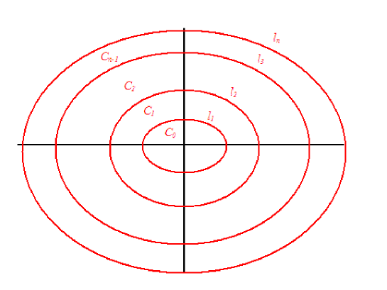
Figure 12: The Gribov horizons

These regions are separated by lines $l_{1},l_{2},l_{3},...,l_{n}$ on which the Faddeev-Popov operator has zero energy solutions. The meaning of Fig.12 is as follows. In the region $C_{0}$ all eigenvalues of the Faddeev-Popov operator are positive, i.e. $-\partial_{\mu}\left(\partial_{\mu}\cdot+\left[A_{\mu},\cdot\right]\right)>0$. At the boundary $l_{1}$ of the region $C_{0}$ the first vanishing eigenvalue appears, namely on $l_{1}$ the Faddeev-Popov operator possesses a normalizable zero mode $\chi$

$$\partial_{\mu}\left(\partial_{\mu}\chi+\left[A_{\mu},\chi\right]\right)=0\;.$$ (144)

In the region $C_{1}$ the Faddeev-Popov operator has one bound state, i.e. one negative energy solution. At the boundary $l_{2}$, a zero eigenvalue reappears. In the region $C_{2}\;$the Faddeev-Popov operator has two bound states, i.e. two negative energy solutions. On $l_{3}$ a zero eigenvalue shows up again, and so on. The boundaries $l_{1},\;l_{2},\;l_{3},\;....,\;l_{n}$,  on which the Faddeev-Popov operator has zero eigenvalues are called Gribov horizons. In particular, the boundary $l_{1}$ where the first vanishing eigenvalue appears is called the first horizon.

• Remark

  It is useful to emphasize that in the region $C_{0}$ the Faddeev-Popov operator has only positive eigenvalues. Therefore, this region can be defined as the set of all transverse fields for which the Faddeev-Popov operator is positive definite, namely

  $$C_{0}=\{A_{\mu},\;\partial A=0,\;-\partial_{\mu}\left(\partial_{\mu}\cdot+\left[A_{\mu},\cdot\right]\right)>0\}\;.$$

• Remark

  In order to obtain a better understanding of the notion of the Gribov horizons, let us remark that there is a close relationship between the horizons and the existence of Gribov copies. In part I, we have discussed the existence of equivalent fields by considering finite gauge transformations

  $$\widetilde{A}_{\mu}={S}^{\dagger}\partial_{\mu}{S}+S^{\dagger}A_{\mu}{S}\;.$$ (145)

  The requirement that the field $\widetilde{A}_{\mu}$ obeys the same transversality condition as $A_{\mu}$

  $$\partial\widetilde{A}=\partial A=0\;,$$ (146)

  yields the equation

  $$\partial_{\mu}S^{\dagger}\partial_{\mu}{S+S}^{\dagger}\partial_{\mu}\partial_{\mu}{S+\partial}_{\mu}S^{\dagger}A_{\mu}{S+}S^{\dagger}A_{\mu}{\partial}_{\mu}{S=0\;.}$$ (147)

  For $S$ close to unit, $S=1+\alpha,$ $\alpha\ll 1$, expression $\left(\ref{ho5}\right)$ reduces to

  $$\partial_{\mu}\left(\partial_{\mu}\alpha+\left[A_{\mu},\alpha\right]\right)=0\;.$$ (148)

  We see therefore that the condition for the existence of an equivalent field $\widetilde{A}_{\mu}$ close to $A_{\mu}$, i.e.

  $$\widetilde{A}_{\mu}=A_{\mu}+\left(\partial_{\mu}\alpha+\left[A_{\mu},\alpha\right]\right)\;,$$ (149)

  relies on the existence of a zero mode for the Faddeev-Popov operator.

• Remark

  The transversality condition of the Landau gauge, $\partial_{\mu}A_{\mu}=0$, implies that the space-time derivative $\partial_{\mu}$ and the covariant derivative $D_{\mu}(A)=\left(\partial_{\mu}\cdot+\left[A_{\mu},\cdot\right]\right)$ obey the following commutation relation

  $$\partial_{\mu}D_{\mu}(A)=D_{\mu}(A)\partial_{\mu}\;.$$ (150)

  As a consequence, the Faddeev-Popov operator $\mathcal{M}=-\partial_{\mu}D_{\mu}(A)$ turns out to be Hermitian, $\mathcal{M}=\mathcal{M}^{\dagger}$. Its eigenvalues are thus real. In fact, integrating by parts, one has

  $$\int d^{4}x\left(\left(\partial_{\mu}D_{\mu}\psi\right)^{a}\right)^{\dagger}\varphi^{a} = \int d^{4}x\left(\partial_{\mu}\partial_{\mu}\psi^{a\dagger}+f^{abc}A_{\mu}^{b}\partial_{\mu}\psi^{c\dagger}\right)\varphi^{a}$$ (151)

  $$= \int d^{4}x\left(\psi^{a\dagger}\partial_{\mu}\partial_{\mu}\varphi^{a}-f^{abc}\psi^{c\dagger}A_{\mu}^{b}\partial_{\mu}\varphi^{a}\right)$$

  $$= \int d^{4}x\left(\psi^{a\dagger}\partial_{\mu}\partial_{\mu}\varphi^{a}+f^{abc}\psi^{a\dagger}A_{\mu}^{b}\partial_{\mu}\varphi^{c}\right)$$

  $$= \int d^{4}x\psi^{a\dagger}\left(\partial_{\mu}D_{\mu}\varphi^{a}\right)\;.$$

3.2 Example of a zero mode of the Faddeev-Popov operator

It is useful to provide here an example of a normalizable zero mode of the Faddeev-Popov operator. We shall work in three dimensions, the gauge group being $SU(2)$. The aim is to obtain a normalizable zero mode $\chi$, solution of

$$\overrightarrow{\nabla}^{2}\chi+\left[A_{i},\partial_{i}\chi\right]=0\;.$$ (152)

We shall follow Henyey’s strategy [2], see also [6], and write

$$\overrightarrow{A}=i\overrightarrow{a}\sigma_{3}\;,\;\;\;\partial_{i}A_{i}=0\;.$$ (153)

Adopting polar coordinates, see App.D, we shall set

$$\overrightarrow{a}=a(r,\theta)\overrightarrow{e}_{\varphi}\;.\;\;\;$$ (154)

We look now at a zero mode $\chi$ of the form

$$\chi=\alpha(r,\theta)\left(\sigma_{1}\cos\varphi+\sigma_{2}\sin\varphi\right)\;.$$ (155)

From

$$\left[\sigma_{i},\sigma_{j}\right]=2i\varepsilon_{ijk}\sigma_{k}\;,$$ (156)

it follows

$$\left[\sigma_{1},\sigma_{2}\right]=2i\sigma_{3}\;,\;\;\;\;\;\;\;\left[\sigma_{3},\sigma_{1}\right]=2i\sigma_{2}\;,\;\;\;\;\;\;\;\;\left[\sigma_{3},\sigma_{2}\right]=-2i\sigma_{1}\;.$$ (157)

Therefore

$$\left[A_{i},\partial_{i}\chi\right] = i\;\left[\sigma_{3},\sigma_{1}\right]a_{i}\partial_{i}\left(\alpha\cos\varphi\right)+i\;\left[\sigma_{3},\sigma_{2}\right]a_{i}\partial_{i}\left(\alpha\sin\varphi\right)$$

$$= -2\sigma_{2}a_{i}\partial_{i}\left(\alpha\cos\varphi\right)+2\sigma_{1}a_{i}\partial_{i}\left(\alpha\sin\varphi\right)$$

$$= -2\sigma_{2}\frac{a}{r\sin\theta}\frac{\partial\left(\alpha\cos\varphi\right)}{\partial\varphi}+2\sigma_{1}\frac{a}{r\sin\theta}\frac{\partial\left(\alpha\sin\varphi\right)}{\partial\varphi}\;.$$

Setting

$$\alpha(r,\theta)=rb(r)\sin\theta\;,$$ (159)

we get

$$\left[A_{i},\partial_{i}\chi\right]=2ab\sin\varphi\sigma_{2}+2ab\cos\varphi\sigma_{1}\;.$$ (160)

Also,

$$\overrightarrow{\nabla}^{2}\chi = \frac{1}{r^{2}}\frac{\partial}{\partial r}\left(r^{2}\frac{\partial\chi}{\partial r}\right)+\frac{1}{r^{2}\sin\theta}\frac{\partial}{\partial\theta}\left(\sin\theta\frac{\partial\chi}{\partial\theta}\right)+\frac{1}{r^{2}\sin^{2}\theta}\frac{\partial^{2}\chi}{\partial\varphi^{2}}\;$$ (161)

$$= \sin\theta\left(\sigma_{1}\cos\varphi+\sigma_{2}\sin\varphi\right)\frac{1}{r^{2}}\frac{\partial}{\partial r}\left(r^{2}\frac{\partial\left(rb(r)\right)}{\partial r}\right)$$

$$+\left(\sigma_{1}\cos\varphi+\sigma_{2}\sin\varphi\right)\frac{b(r)}{r\sin\theta}\frac{\partial}{\partial\theta}\left(\sin\theta\frac{\partial\sin\theta}{\partial\theta}\right)$$

$$+\frac{b(r)}{r\sin\theta}\frac{\partial^{2}\left(\sigma_{1}\cos\varphi+\sigma_{2}\sin\varphi\right)\;}{\partial\varphi^{2}}\;$$

$$= \sin\theta\left(\sigma_{1}\cos\varphi+\sigma_{2}\sin\varphi\right)\frac{1}{r^{2}}\frac{\partial}{\partial r}\left(r^{3}b^{\prime}+r^{2}b\right)$$

$$+\left(\sigma_{1}\cos\varphi+\sigma_{2}\sin\varphi\right)\frac{b}{r\sin\theta}\frac{\partial}{\partial\theta}\left(\sin\theta\cos\theta\right)$$

$$-\frac{b(r)}{r\sin\theta}\left(\sigma_{1}\cos\varphi+\sigma_{2}\sin\varphi\right)$$

$$= \sin\theta\left(\sigma_{1}\cos\varphi+\sigma_{2}\sin\varphi\right)\frac{1}{r^{2}}(4r^{2}b^{\prime}+r^{3}b^{\prime\prime}+2rb)$$

$$+\left(\sigma_{1}\cos\varphi+\sigma_{2}\sin\varphi\right)\frac{b}{r\sin\theta}\left(\cos^{2}\theta-\sin^{2}\theta\right)$$

$$-\frac{b(r)}{r\sin\theta}\left(\sigma_{1}\cos\varphi+\sigma_{2}\sin\varphi\right)$$

$$= (4b^{\prime}+rb^{\prime\prime})\sin\theta\left(\sigma_{1}\cos\varphi+\sigma_{2}\sin\varphi\right)$$

$$+\frac{b}{r}\left(2\sin\theta+\frac{\left(\cos^{2}\theta-\sin^{2}\theta\right)}{\sin\theta}\right)\left(\sigma_{1}\cos\varphi+\sigma_{2}\sin\varphi\right)$$

$$-\frac{b(r)}{r\sin\theta}\left(\sigma_{1}\cos\varphi+\sigma_{2}\sin\varphi\right)$$

$$= (4b^{\prime}+rb^{\prime\prime})\sin\theta\left(\sigma_{1}\cos\varphi+\sigma_{2}\sin\varphi\right)$$

$$+\frac{b}{r\sin\theta}\left(\sigma_{1}\cos\varphi+\sigma_{2}\sin\varphi\right)-\frac{b(r)}{r\sin\theta}\left(\sigma_{1}\cos\varphi+\sigma_{2}\sin\varphi\right)$$

$$= (4b^{\prime}+rb^{\prime\prime})\sin\theta\left(\sigma_{1}\cos\varphi+\sigma_{2}\sin\varphi\right)$$

Finally,

$$\overrightarrow{\nabla}^{2}\chi=(4b^{\prime}+rb^{\prime\prime})\sin\theta\left(\sigma_{1}\cos\varphi+\sigma_{2}\sin\varphi\right)\;.$$ (162)

The equation $\left(\ref{ho8}\right)$ is thus equivalent to

$$(4b^{\prime}+rb^{\prime\prime})\sin\theta\left(\sigma_{1}\cos\varphi+\sigma_{2}\sin\varphi\right)+2ab\sin\varphi\sigma_{2}+2ab\cos\varphi\sigma_{1}=0\;,$$ (163)

which yields

$$(4b^{\prime}+rb^{\prime\prime})\sin\theta+2ab=0\;.$$ (164)

Following Henyey [2], for $a$ we obtain

$$a=-\frac{r}{2b}\sin\theta\left(b^{\prime\prime}+\frac{4b^{\prime}}{r}\right)\;.$$ (165)

We now look for a function $b$ which yields a field configuration $a(r,\theta)$ which is regular at the origin, $r=0$, and which decays faster than $1/r$ for $r\rightarrow\infty$. As done in Part I, for $b$ we choose

$$b(r)=\frac{k}{\left(r^{2}+r_{0}^{2}\right)^{3/2}}\;,\;\;\;\;\;k\;\;\;\mathrm{const.\;\;and\;}r_{0}\neq 0\;.$$ (166)

Therefore, for $a(r,\theta)$ we find [6]

$$a(r,\theta) = -\frac{r}{2}\left(r^{2}+r_{0}^{2}\right)^{3/2}\sin\theta\left(-3\frac{\partial}{\partial r}\frac{r}{\left(r^{2}+r_{0}^{2}\right)^{5/2}}-\frac{12}{\left(r^{2}+r_{0}^{2}\right)^{5/2}}\right)$$ (167)

$$= -\frac{r}{2}\left(r^{2}+r_{0}^{2}\right)^{3/2}\sin\theta\left(15\frac{r^{2}}{\left(r^{2}+r_{0}^{2}\right)^{7/2}}-\frac{15}{\left(r^{2}+r_{0}^{2}\right)^{5/2}}\right)$$

$$= \frac{15}{2}\frac{rr_{0}^{2}}{\left(r^{2}+r_{0}^{2}\right)^{2}}\sin\theta\;.$$

Observe that

$$a(r,\theta) \rightarrow 0\;\;\mathrm{for\;\;}r\rightarrow 0\;,$$ (168)

$$a(r,\theta) \sim \frac{1}{r^{3}}\;\;\mathrm{for\;}r\rightarrow\infty\;.$$

It remains to check that $\chi$ is a normalizable zero mode with respect to the scalar product

$$\left\langle X\mid Y\right\rangle=Tr\int d^{3}xX^{\dagger}Y\;.$$ (169)

From

$$\chi=rb\sin\theta\left(\sigma_{1}\cos\varphi+\sigma_{2}\sin\varphi\right)\;,$$ (170)

we have

$$\chi^{\dagger}=rb\sin\theta\left(\sigma_{1}\cos\varphi+\sigma_{2}\sin\varphi\right)\;,$$ (171)

and

$$Tr\left(\chi^{\dagger}\chi\right)=2r^{2}b^{2}\sin^{2}\theta\;.$$ (172)

Thus

$$\left\langle\chi\mid\chi\right\rangle=2\int d^{3}xr^{2}b^{2}\sin^{2}\theta=4\pi k^{2}\int_{0}^{\pi}\sin^{3}\theta d\theta\int_{0}^{\infty}dr\frac{r^{4}}{\left(r^{2}+r_{0}^{2}\right)^{3}}<\infty\;,$$ (173)

showing that we have found a normalizable zero mode of the Faddeev-Popov operator.

• Summary

  For the zero mode we have

  $$\overrightarrow{\nabla}^{2}\chi+\left[A_{i},\partial_{i}\chi\right]=0\;,$$ (174)

  with

  $$\overrightarrow{A}=i\overrightarrow{a}\sigma_{3}\;,\;\;\;\partial_{i}A_{i}=0\;,$$

  $$\overrightarrow{a}=a(r,\theta)\overrightarrow{e}_{\varphi}\;,$$ (175)

  and

  $$\chi=rb\sin\theta\left(\sigma_{1}\cos\varphi+\sigma_{2}\sin\varphi\right)\;,$$ (176)

  $$b(r)=\frac{k}{\left(r^{2}+r_{0}^{2}\right)^{3/2}}\;,\;\;\;\;\;k\;\mathrm{{\mathrm{const.}}\mathrm{\;\;and\;}r_{0}\neq 0\;.}$$ (177)

  $$\left\langle\chi\mid\chi\right\rangle=\int d^{3}xTr\left(\chi^{\dagger}\chi\right)<\infty\;\;.$$ (178)

  For $a(r,\theta)$  one finds

  $$a=-\frac{r}{2b}\sin\theta\left(b^{\prime\prime}+\frac{4b^{\prime}}{r}\right)\;=\frac{15}{2}\frac{rr_{0}^{2}}{\left(r^{2}+r_{0}^{2}\right)^{2}}\sin\theta\;,$$ (179)

  $$a(r,\theta)\rightarrow 0\;\;\mathrm{for\;\;}r\rightarrow 0\;,$$ (180)

  $$a(r,\theta)\sim\frac{1}{r^{3}}\;\;\mathrm{for\;}r\rightarrow\infty\;.$$

  Also, $\overrightarrow{a}$ is transverse

  $$\partial_{i}a_{i}=\frac{1}{r\sin\theta}\frac{\partial a(r,\theta)}{\partial\varphi}=0\;.$$ (181)

3.3 An important statement

Let us prove the following statement [1]:

• Statement

  For any field located within the region $C_{1}$, close to the boundary $l_{1}$, there is an equivalent field within the region $C_{0}$, close to the same boundary $l_{1}$, see Fig.13

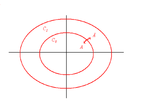
Figure 13: The Equivalent Fields

Let $A_{\mu}$ be the field located in $C_{0}$, close to the first horizon $l_{1}$. We write

$$A_{\mu}=C_{\mu}+a_{\mu}\;,\;\;\;\;\;a_{\mu}\;\mathrm{small\;with\;respect\;to\;}C_{\mu}\;,$$ (182)

where the transverse field $C_{\mu}$, $\partial C=0$, lies on the Gribov horizon $l_{1}$, i.e. it exists a normalizable zero mode $\varphi_{0}$ such that

$$\partial_{\mu}\left(\partial_{\mu}\varphi_{0}+\left[C_{\mu},\varphi_{0}\right]\right)=0\;.$$ (183)

• Remark

  Notice also that, by definition, the field $A_{\mu}$ is located in the region $C_{0}$, so that

  $$-\partial_{\mu}\left(\partial_{\mu}\cdot+\left[A_{\mu},\cdot\right]\right)>0\;.$$ (184)

The eigenvalues problem for the Faddeev-Popov operator corresponding to the field $A_{\mu}$ can be easily handled by means of the perturbation theory of quantum mechanics. Let us look indeed at the eigenvalues equation

$$-\partial_{\mu}\left(\partial_{\mu}\psi+\left[C_{\mu}+a_{\mu},\psi\right]\right)=\epsilon(a)\psi\;,$$ (185)

i.e.

$$-\left(\partial^{2}\psi+\left[C_{\mu},\partial_{\mu}\psi\right]+\partial_{\mu}\left[a_{\mu},\psi\right]\right)=\epsilon(a)\psi\;.$$ (186)

One might think of $a_{\mu}$ as a small perturbation. Accordingly, the shift $\epsilon(a)$ of the eigenvalue of the Faddeev-Popov operator from zero can be obtained in perturbation theory by evaluating the expectation value of the term $\partial_{\mu}\left[a_{\mu},\cdot\right]$, namely

$$\epsilon(a)=-\frac{\left\langle\varphi_{0}\mid\partial_{\mu}\left[a_{\mu},\varphi_{0}\right]\right\rangle}{\left\langle\varphi_{0}\mid\varphi_{0}\right\rangle}=-\frac{Tr\int d^{4}x\left(\varphi_{0}\partial_{\mu}\left[a_{\mu},\varphi_{0}\right]\right)}{Tr\int d^{4}x\left(\varphi_{0}\varphi_{0}\right)}\;.$$ (187)

Since $\partial_{\mu}\left(\partial_{\mu}\varphi_{0}+\left[C_{\mu},\varphi_{0}\right]\right)=0$, it is easily verified that the field

$$\widetilde{A}_{\mu}=A_{\mu}+D_{\mu}(C)\varphi_{0}\;,$$ (188)

has the same divergence of $A_{\mu}$. In fact

$$\partial_{\mu}\widetilde{A}_{\mu}=\partial_{\mu}A_{\mu}+\partial_{\mu}D_{\mu}(C)\varphi_{0}=\partial_{\mu}A_{\mu}\;.\;$$ (189)

The fields $\widetilde{A}_{\mu}$ and $A_{\mu}$ can thus define equivalent fields. For that, we have to find a gauge transformation $S$ such that

$$\widetilde{A}_{\mu}={S}^{\dagger}\partial_{\mu}{S}+S^{\dagger}A_{\mu}{S}\;.$$ (190)

We shall look at $S$ close to unit, in the form

$$S=1+\alpha+\frac{1}{2}\alpha^{2}+....$$ (191)

Also

$$S^{\dagger}=1-\alpha+\frac{1}{2}\alpha^{2}+....$$ (192)

Indeed

$$SS^{\dagger} = \left(1+\alpha+\frac{1}{2}\alpha^{2}\right)\left(1-\alpha+\frac{1}{2}\alpha^{2}\right)+O(\alpha^{3})$$ (193)

$$= 1-\alpha+\frac{1}{2}\alpha^{2}+\alpha-\alpha^{2}+\frac{1}{2}\alpha^{2}+O(\alpha^{3})$$

$$= 1+O(\alpha^{3})\;.$$

For $\widetilde{A}_{\mu}$ we get

$$\widetilde{A}_{\mu} = \left(1-\alpha+\frac{1}{2}\alpha^{2}\right)A_{\mu}\left(1+\alpha+\frac{1}{2}\alpha^{2}\right)+\left(1-\alpha+\frac{1}{2}\alpha^{2}\right)\partial_{\mu}\left(1+\alpha+\frac{1}{2}\alpha^{2}\right)$$ (194)

$$= \left(1-\alpha+\frac{1}{2}\alpha^{2}\right)\left(A_{\mu}+A_{\mu}\alpha+\frac{1}{2}A_{\mu}\alpha^{2}\right)$$

$$+\left(1-\alpha+\frac{1}{2}\alpha^{2}\right)\left(\partial_{\mu}\alpha+\frac{1}{2}\left(\partial_{\mu}\alpha\right)\alpha+\frac{1}{2}\alpha\left(\partial_{\mu}\alpha\right)\right)$$

$$= A_{\mu}+A_{\mu}\alpha+\frac{1}{2}A_{\mu}\alpha^{2}-\alpha A_{\mu}-\alpha A_{\mu}\alpha+\frac{1}{2}\alpha^{2}A_{\mu}+\partial_{\mu}\alpha$$

$$+\frac{1}{2}\left(\partial_{\mu}\alpha\right)\alpha+\frac{1}{2}\alpha\left(\partial_{\mu}\alpha\right)-\alpha\partial_{\mu}\alpha+O(\alpha^{3})$$

$$= A_{\mu}+D_{\mu}(A)\alpha+\frac{1}{2}\left(\partial_{\mu}\alpha\right)\alpha-\frac{1}{2}\alpha\left(\partial_{\mu}\alpha\right)$$

$$+\frac{1}{2}A_{\mu}\alpha^{2}-\alpha A_{\mu}\alpha+\frac{1}{2}\alpha^{2}A_{\mu}+O(\alpha^{3})\;.$$

From

$$\left[\alpha,\partial_{\mu}\alpha+\left[A_{\mu},\alpha\right]\right]=\alpha\left(\partial_{\mu}\alpha\right)-\left(\partial_{\mu}\alpha\right)\alpha+\alpha A_{\mu}\alpha-\alpha^{2}A_{\mu}-A_{\mu}\alpha^{2}+\alpha A_{\mu}\alpha\;,$$ (195)

it follows

$$\widetilde{A}_{\mu}=A_{\mu}+D_{\mu}(A)\alpha-\frac{1}{2}\left[\alpha,\partial_{\mu}\alpha+\left[A_{\mu},\alpha\right]\right]+O(\alpha^{3})\;.$$ (196)

• Remark

  We must retain the second order term in the equation $\left(\ref{s11}\right)$  otherwise, from

  $$S=1+\alpha\;,$$ (197)

  we would obtain

  $$\widetilde{A}_{\mu}=A_{\mu}+D_{\mu}(A)\alpha\;.$$ (198)

  Condition $\left(\ref{s9}\right)$, $\partial\widetilde{A}=\partial A$, would thus imply

  $$\partial_{\mu}D_{\mu}(A)\alpha=0\;,$$ (199)

  which has no solution for $\alpha$ since $A_{\mu}$ is not located on a horizon, see eq.$\left(\ref{s4}\right)$.

From equation $\left(\ref{s16}\right)$ one obviously has

$$D_{\mu}(C)\varphi_{0}=D_{\mu}(A)\alpha-\frac{1}{2}\left[\alpha,\partial_{\mu}\alpha+\left[A_{\mu},\alpha\right]\right]+O(\alpha^{3})\;.$$ (200)

Tacking the divergence of both sides of eq.$\left(\ref{s20}\right)$, we obtain the condition to be fulfilled in order that $A_{\mu}\;$and $\widetilde{A}_{\mu}$ have the same divergence, $\partial\widetilde{A}=\partial A$, i.e.

$$\partial_{\mu}D_{\mu}(A)\alpha-\frac{1}{2}\partial_{\mu}\left[\alpha,\partial_{\mu}\alpha+\left[A_{\mu},\alpha\right]\right]=0\;.$$ (201)

This condition can be analyzed iteratively by setting

$$\alpha = \varphi_{0}+\widetilde{\alpha}\;,\,\,\,\,\,\,\,\,\,\,\,\,\,\,\,\;\widetilde{\alpha}\;\mathrm{small\;with\;respect\;to\;}\varphi_{0}\;,$$

$$A_{\mu} = C_{\mu}+a_{\mu}\;,\;\;\;\;a_{\mu}\;\mathrm{small\;with\;respect\;to\;}A_{\mu}\;,$$ (202)

It is useful to introduce an expansion parameter $\lambda$ which we shall set to one at the end

$$\alpha = \lambda\varphi_{0}+\lambda^{2}\widetilde{\alpha}\;,$$

$$A_{\mu} = C_{\mu}+\lambda a_{\mu}\;.\,$$ (203)

Condition $\left(\ref{s21}\right)$ gives

$$\partial^{2}\left(\lambda\varphi_{0}+\lambda^{2}\widetilde{\alpha}\right)+ \partial_{\mu}\left[\;C_{\mu}+\lambda a_{\mu},\lambda\varphi_{0}+\lambda^{2}\widetilde{\alpha}\right]=\frac{1}{2}\partial_{\mu}\left[\lambda\varphi_{0}+\lambda^{2}\widetilde{\alpha}\;,\partial_{\mu}\left(\lambda\varphi_{0}+\lambda^{2}\widetilde{\alpha}\right)\right]$$

$$+\frac{1}{2}\partial_{\mu}\left[\lambda\varphi_{0}+\lambda^{2}\widetilde{\alpha}\;,\left[C_{\mu}+\lambda a_{\mu},\lambda\varphi_{0}+\lambda^{2}\widetilde{\alpha}\right]\right]$$

so that, up to terms of the order $\lambda^{4}$

$$\lambda^{2}\partial_{\mu}\left(\partial_{\mu}\widetilde{\alpha}+\left[\;C_{\mu},\widetilde{\alpha}\right]\right)+\lambda^{2}\partial_{\mu}\left[\;a_{\mu},\varphi_{0}\right]+\lambda^{3}\partial_{\mu}\left[\;a_{\mu},\widetilde{\alpha}\right]=\frac{\lambda^{2}}{2}\partial_{\mu}\left[\varphi_{0}\;,\partial_{\mu}\varphi_{0}+\left[C_{\mu},\varphi_{0}\right]\right]$$

$$+\frac{\lambda^{3}}{2}\partial_{\mu}\left[\varphi_{0},\partial_{\mu}\widetilde{\alpha}+\left[C_{\mu},\widetilde{\alpha}\right]\right]+\frac{\lambda^{3}}{2}\partial_{\mu}\left[\widetilde{\alpha},\partial_{\mu}\varphi_{0}+\left[C_{\mu},\varphi_{0}\right]\right]+\frac{\lambda^{3}}{2}\partial_{\mu}\left[\varphi_{0},\left[a_{\mu},\varphi_{0}\right]\right]+O(\lambda^{4})\;.$$

(205)

In particular, to the first order $\lambda^{2}$, we find

$$\partial_{\mu}D_{\mu}(C)\widetilde{\alpha}+\partial_{\mu}\left[\;a_{\mu},\varphi_{0}\right]=\frac{1}{2}\partial_{\mu}\left[\varphi_{0},D_{\mu}(C)\varphi_{0}\right]\;,$$ (206)

from which it follows that

$$Tr\int d^{4}x\left(\varphi_{0}\partial_{\mu}D_{\mu}(C)\widetilde{\alpha}+\varphi_{0}\partial_{\mu}\left[\;a_{\mu},\varphi_{0}\right]\right)=\frac{1}{2}Tr\int d^{4}x\left(\varphi_{0}\partial_{\mu}\left[\varphi_{0},D_{\mu}(C)\varphi_{0}\right]\right)\;.$$ (207)

Moreover, due to property $\partial_{\mu}D_{\mu}(C)=D_{\mu}(C)\partial_{\mu}$, we have

$$Tr\int d^{4}x\varphi_{0}\partial_{\mu}D_{\mu}(C)\widetilde{\alpha}=Tr\int d^{4}x\left(\partial_{\mu}D_{\mu}(C)\varphi_{0}\right)\widetilde{\alpha}=0\;.$$ (208)

As a consequence, condition $\left(\ref{s2226}\right)$ reads

$$Tr\int d^{4}x\left(\varphi_{0}\partial_{\mu}\left[\;a_{\mu},\varphi_{0}\right]\right)=\frac{1}{2}Tr\int d^{4}x\left(\varphi_{0}\partial_{\mu}\left[\varphi_{0},D_{\mu}(C)\varphi_{0}\right]\right)\;.$$ (209)

• Summary

  The fields $A_{\mu}\;$and $\widetilde{A}_{\mu}$ 

  $$\widetilde{A}_{\mu}=A_{\mu}+D_{\mu}(C)\varphi_{0}\;,$$ (210)

  are equivalent fields

  $$\partial_{\mu}\widetilde{A}_{\mu}=\partial_{\mu}A_{\mu}+\partial_{\mu}D_{\mu}(C)\varphi_{0}=\partial_{\mu}A_{\mu}\;.\;$$ (211)

  For the gauge transformation $S$

  $$\widetilde{A}_{\mu}={S}^{\dagger}\partial_{\mu}{S}+S^{\dagger}A_{\mu}{S}\;,$$ (212)

  we have

  $$S=1+\alpha+\frac{1}{2}\alpha^{2}+O(\alpha^{3})\;,$$ (213)

  so that

  $$\widetilde{A}_{\mu}=A_{\mu}+D_{\mu}(A)\alpha-\frac{1}{2}\left[\alpha,\partial_{\mu}\alpha+\left[A_{\mu},\alpha\right]\right]+O(\alpha^{3})\;.$$ (214)

  The condition  $\partial\widetilde{A}=\partial A$ gives

  $$\partial_{\mu}D_{\mu}(A)\alpha=\frac{1}{2}\partial_{\mu}\left[\alpha,\partial_{\mu}\alpha+\left[A_{\mu},\alpha\right]\right]+O(\alpha^{3})\;.$$ (215)

  Setting

  $$\alpha = \varphi_{0}+\widetilde{\alpha}\;,\,\,\,\,\,\,\,\,\,\,\,\,\,\,\,\;\widetilde{\alpha}\;\mathrm{small\;with\;respect\;to\;}\varphi_{0}\;,$$

  $$A_{\mu} = C_{\mu}+a_{\mu}\;,\;\;\;\;a_{\mu}\;\mathrm{small\;with\;respect\;to\;}A_{\mu}\;,$$ (216)

  we obtain, to the first order,

$$\partial_{\mu}D_{\mu}(C)\widetilde{\alpha}+\partial_{\mu}\left[\;a_{\mu},\varphi_{0}\right]=\frac{1}{2}\partial_{\mu}\left[\varphi_{0},D_{\mu}(C)\varphi_{0}\right]\;.$$ (217)

It remains now to check on which side of the horizon $l_{1}$ the equivalent field $\widetilde{A}_{\mu}$ lies. Let us rewrite $\widetilde{A}_{\mu}$ as

$$\widetilde{A}_{\mu}=A_{\mu}+D_{\mu}(C)\varphi_{0}\;=C_{\mu}+a_{\mu}+D_{\mu}(C)\varphi_{0}=C_{\mu}+a_{\mu}^{\prime}\;.$$ (218)

As done before, we evaluate the shift $\epsilon(a^{\prime})$ of the eigenvalue of the Faddeev-Popov operator from zero. Treating the field $a_{\mu}^{\prime}=a_{\mu}+D_{\mu}(C)\varphi_{0}\;$as a perturbation, one obtains

$$\epsilon(a^{\prime})=-\frac{\left\langle\varphi_{0}\mid\partial_{\mu}\left[a_{\mu}^{\prime},\varphi_{0}\right]\right\rangle}{\left\langle\varphi_{0}\mid\varphi_{0}\right\rangle}=-\frac{Tr\int d^{4}x\left(\varphi_{0}\partial_{\mu}\left[a_{\mu},\varphi_{0}\right]+\varphi_{0}\partial_{\mu}\left[D_{\mu}(C)\varphi_{0},\varphi_{0}\right]\right)}{Tr\int d^{4}x\left(\varphi_{0}\varphi_{0}\right)}\;.$$ (219)

Furthermore, from eq.$\left(\ref{sf26}\right)$, it follows

$$\epsilon(a^{\prime})=\frac{Tr\int d^{4}x\left(\varphi_{0}\partial_{\mu}\left[a_{\mu},\varphi_{0}\right]\right)}{Tr\int d^{4}x\left(\varphi_{0}\varphi_{0}\right)}\;=-\epsilon(a)\;.$$ (220)

Thus, if $A_{\mu}$, close to $l_{1}$, is located in $C_{0}$, $\epsilon(a)>0$, there is an equivalent field, $\widetilde{A}_{\mu}=A_{\mu}+D_{\mu}(C)\varphi_{0}$, close to $l_{1}$, which is located in $C_{1}$, $\epsilon(a^{\prime})=-\epsilon(a)<0$. Also, it is worth mentioning that this derivation can be generalized to fields close to any horizon $l_{n}$. This concludes the proof of the statement.

3.4 Restriction of the domain of integration to the first horizon

The previous statement suggests that the domain of integration in the path integral should be restricted to the first horizon, i.e. to the region $C_{0}$ where the Faddeev-Popov operator is positive definite.

• Remark

  More precisely, two additional requirements should be fulfilled to justify the hypothesis that the domain of integration should be restricted to the region $C_{0}$. The first one is that one should be able to prove that not only for small neighborhoods close to the horizons $l_{n}$, but also for any field in the region $C_{n}$ there is an equivalent field in the region $C_{n-1}$. This would ensure that it is always possible to find a chain of gauge transformations which brings a field in the region $C_{n}$ to the corresponding equivalent field in the region $C_{0}$. The second requirement is that one has to be sure that the region $C_{0}$ is free from Gribov copies. We shall come back on these issues later on in the Conclusion. For the time being, we shall assume that the significant range of integration in the path-integral is determined by the region $C_{0}$.

Accordingly, for the partition function $\mathcal{Z}$ we write

$$\mathcal{Z} = \mathcal{N}\int DA_{\mu}DcD\overline{c}\delta(\partial A)e^{-\left(S_{YM}+\int d^{4}x\overline{c}^{a}\partial_{\mu}D_{\mu}^{ab}c^{b}\right)}\mathcal{V}(C_{0})$$ (221)

$$= \mathcal{N}\int DA_{\mu}\delta(\partial A)e^{-S_{YM}}\det\left(-\partial_{\mu}(\partial_{\mu}\delta^{ab}-f^{abc}A_{\mu}^{c})\right)\mathcal{V}(C_{0})\;,$$

where the presence of the factor $\mathcal{V}(C_{0})$ means that the integration is performed only over the region $C_{0}$. In order to characterize the quantity $\mathcal{V}(C_{0})$, we look at the connected two-point ghost function $\left\langle\overline{c}^{a}(x)c^{b}(y)\right\rangle_{\mathrm{c}}$. We have

$$\left\langle\overline{c}^{a}(x)c^{b}(y)\right\rangle_{\mathrm{c}} = \mathcal{N}\int DA_{\mu}DcD\overline{c}\delta(\partial A)\overline{c}^{a}(x)c^{b}(y)e^{-\left(S_{YM}+\int d^{4}x\overline{c}^{a}\partial_{\mu}D_{\mu}^{ab}c^{b}\right)}\mathcal{V}(C_{0})$$

$$= \mathcal{N}\int DA_{\mu}\delta(\partial A)e^{-S_{YM}}\det\left(-\partial_{\mu}D_{\mu}\right)\left[\left(\partial_{\mu}D_{\mu}\right)^{-1}\right]_{xy}^{ab}\mathcal{V}(C_{0})\;.$$

The presence of the factor $\mathcal{V}(C_{0})$ in eq.$\left(\ref{r2}\right)$ implies that $\left\langle\overline{c}^{a}(x)c^{b}(y)\right\rangle_{\mathrm{c}}$ can become large only when approaching the horizon $l_{1}$. On the other hand, the behavior of the two-point ghost function obtained from perturbation theory, i.e. with $\mathcal{V}(C_{0})=1$, is given by

$$\left\langle\overline{c}^{a}(x)c^{b}(y)\right\rangle_{\mathrm{c}} = \delta^{ab}\int\frac{d^{4}k}{\left(2\pi\right)^{4}}\mathcal{G}(k)e^{ik(x-y)}\;,$$

$$\mathcal{G}(k) = \frac{1}{k^{2}}\frac{1}{\left(1-\frac{11g^{2}N}{48\pi^{2}}\log\frac{\Lambda^{2}}{k^{2}}\right)^{\frac{9}{44}}}\;,$$ (223)

where $\Lambda$ is the ultraviolet cutoff and $N$ is the Casimir of the adjoint representation of the gauge group $SU(N)$

$$f^{acd}f^{bcd}=N\delta^{ab}\;.$$ (224)

The expression of $\mathcal{G}(k)$ in eq.$\left(\ref{r3}\right)$ displays two singularities, at $k^{2}=0$ and at $k_{c}^{2}=\Lambda^{2}\exp\left(-\frac{1}{g^{2}}\frac{48\pi^{2}}{11N}\right)$. However, the presence of the factor $\mathcal{V}(C_{0})$ makes it impossible for a singularity of $\mathcal{G}(k)$ to exist at nonvanishing $k$. Indeed, below the singularity position, i.e. for $k^{2}<k_{c}^{2}$, the quantity $\left(1-\frac{11g^{2}N}{48\pi^{2}}\log\frac{\Lambda^{2}}{k^{2}}\right)$ is negative. Thus, for $k^{2}<k_{c}^{2}$, $\mathcal{G}(k)$ becomes complex, indicating that the Faddeev-Popov operator $\left(-\partial_{\mu}D_{\mu}\right)$ has ceased to be a positive defined quantity, namely one has left the region $C_{0}$. It remains the singularity at $k^{2}=0$. This singularity has a simple interpretation. It means that we are approaching the boundary $l_{1}$ of $C_{0}$. In other words, at $k^{2}=0$ we feel the fields on the horizon $l_{1}$.

Therefore, following [1], a possible characterization of the factor $\mathcal{V}(C_{0})$ can be obtained by computing the connected two-point ghost function and by requiring that it has no poles at nonvanishing $k$.

• Remark

  For a better understanding of the previous statement about the characterization of the factor $\mathcal{V}(C_{0})$, it is useful to remind here that the region $C_{0}$ is defined as the set of all transverse connections for which the Faddeev-Popov operator is positive definite, namely

  $$C_{0}=\{A_{\mu},\;\partial A=0,\;-\partial_{\mu}\left(\partial_{\mu}\delta^{ab}-f^{abc}A_{\mu}^{c}\right)>0\}\;.$$

  In the region $C_{0}$, the Faddeev-Popov operator is invertible, its inverse $\left[-\partial_{\mu}\left(\partial_{\mu}\delta^{ab}-f^{abc}A_{\mu}^{c}\right)\right]^{-1}$ becoming large only when approaching the horizon $l_{1}$, due to the existence of a zero mode.
  Therefore, denoting by $\mathcal{G}(k;A)$ the color singlet Fourier transform of $\left[-\partial_{\mu}\left(\partial_{\mu}\delta^{ab}-f^{abc}A_{\mu}^{c}\right)\right]^{-1}$,

  $$\mathcal{G}(k;A)=\sum_{ab}\frac{\delta^{ab}}{N^{2}-1}<k\mid\left[-\partial_{\mu}\left(\partial_{\mu}\delta^{ab}-f^{abc}A_{\mu}^{c}\right)\right]^{-1}\mid k>\;,$$ (225)

  we shall require that $\mathcal{G}(k;A)$ has no poles for a given nonvanishing value of the momentum $k$, except for the singularity at $k=0$, corresponding to the Gribov horizon $l_{1}$. Finally, we remark that expression $\left(\ref{cosi}\right)$ can be evaluated order by order in perturbation theory. It can be obtained by computing the connected two-point ghost function in the background of the gauge field $A_{\mu}^{a}$, which plays the role of an external field. This will be task of the next section.

3.5 Characterization of $\mathcal{V}(C_{0})$

In order to characterize $\mathcal{V}(C_{0})$, we start with the expression of the connected, color singlet, two-point ghost function

$$\sum_{ab}\frac{\delta^{ab}\left\langle\overline{c}^{a}(x)c^{b}(y)\right\rangle_{\mathrm{c}}}{N^{2}-1} = \mathcal{N}\int DA_{\mu}DcD\overline{c}\delta(\partial A)\frac{\overline{c}^{a}(x)c^{a}(y)}{\left(N^{2}-1\right)}e^{-\left(S_{YM}+\int d^{4}x\overline{c}^{a}\partial_{\mu}D_{\mu}^{ab}c^{b}\right)}$$

$$= \mathcal{N}\int DA_{\mu}\delta(\partial A)e^{-S_{YM}}\mathcal{G}(x,y;A)\;,$$

where $\mathcal{G}(x,y;A)$ stands for the connected ghost two-point function with the gauge field $A_{\mu}^{a}$ considered as an external classical field, namely

$$\mathcal{G}(x,y;A) = \frac{1}{N^{2}-1}\int DcD\overline{c}\;\overline{c}^{a}(x)c^{a}(y)e^{-\int d^{4}x\overline{c}^{a}\partial_{\mu}D_{\mu}^{ab}c^{b}}\;.$$

We shall evaluate $\mathcal{G}(x,y;A)$ up to the second order in perturbation theory. Making use of the Wick theorem, we obtain

$$\left\langle\overline{c}^{a}(x)c^{b}(y)\right\rangle_{\mathrm{c}}=\left\langle\overline{c}_{0}^{a}(x)c_{0}^{b}(y)\left(1+\int d^{4}x_{1}\left(\partial_{x_{1}}^{\mu}\overline{c}_{0}^{m}(x_{1})\right)f^{mnp}A_{\mu}^{n}(x_{1})c_{0}^{p}(x_{1})\right.\right.$$ (228)

$$\left.\left.+\frac{1}{2}\int d^{4}x_{1}d^{4}x_{2}\left(\partial_{x_{1}}^{\mu}\overline{c}_{0}^{m}(x_{1})\right)f^{mnp}A_{\mu}^{n}(x_{1})c_{0}^{p}(x_{1})\left(\partial_{x_{2}}^{\nu}\overline{c}_{0}^{q}(x_{2})\right)f^{qrt}A_{\mu}^{r}(x_{2})c_{0}^{t}(x_{2})\right)\right\rangle_{\mathrm{c}}$$

(229)

where $\overline{c}_{0}^{a}(x)$, $c_{0}^{b}(y)$ stand for free fields. Performing the Wick contraction, yields

$$\left\langle\overline{c}^{a}(x)c^{b}(y)\right\rangle_{\mathrm{c}}=\left\langle\overline{c}_{0}^{a}(x)c_{0}^{b}(y)\right\rangle-\int d^{4}x_{1}f^{mnp}A_{\mu}^{n}(x_{1})\left\langle\overline{c}_{0}^{a}(x)c_{0}^{p}(x_{1})\right\rangle\partial_{x_{1}}^{\mu}\left\langle\overline{c}_{0}^{m}(x_{1})c_{0}^{b}(y)\right\rangle$$ (230)

$$+\int d^{4}x_{1}d^{4}x_{2}f^{mnp}A_{\mu}^{n}(x_{1})f^{qrt}A_{\nu}^{r}(x_{2})\left\langle\overline{c}_{0}^{a}(x)c_{0}^{p}(x_{1})\right\rangle\partial_{x_{1}}^{\mu}\left\langle\overline{c}_{0}^{m}(x_{1})c_{0}^{t}(x_{2})\right\rangle\partial_{x_{2}}^{\nu}\left\langle\overline{c}_{0}^{q}(x_{2})c_{0}^{b}(y)\right\rangle$$

(231)

From

$$\left\langle\overline{c}_{0}^{a}(x)c_{0}^{b}(y)\right\rangle=\delta^{ab}\mathcal{G}_{0}(x-y)\;,$$ (232)

with $\mathcal{G}_{0}(x-y)$ being the free ghost propagator, we get

$$\left\langle\overline{c}^{a}(x)c^{b}(y)\right\rangle_{\mathrm{c}}=\delta^{ab}\mathcal{G}_{0}(x-y)-\int d^{4}x_{1}\mathcal{G}_{0}(x-x_{1})\partial_{x_{1}}^{\mu}\mathcal{G}_{0}(x_{1}-y)f^{bna}A_{\mu}^{n}(x_{1})$$ (233)

$$+\int d^{4}x_{1}d^{4}x_{2}\mathcal{G}_{0}(x-x_{1})\partial_{x_{1}}^{\mu}\mathcal{G}_{0}(x_{1}-x_{2})\partial_{x_{2}}^{\nu}\mathcal{G}_{0}(x_{2}-y)f^{tna}A_{\mu}^{n}(x_{1})f^{brt}A_{\nu}^{r}(x_{2})\;.$$

(234)

Finally, for $\mathcal{G}(x,y;A)$ we obtain

$$\mathcal{G}(x,y;A)=\mathcal{G}_{0}(x-y)-\frac{1}{N^{2}-1}\int d^{4}x_{1}\mathcal{G}_{0}(x-x_{1})\partial_{x_{1}}^{\mu}\mathcal{G}_{0}(x_{1}-y)f^{ana}A_{\mu}^{n}(x_{1})$$ (235)

$$+\frac{1}{N^{2}-1}\int d^{4}x_{1}d^{4}x_{2}\mathcal{G}_{0}(x-x_{1})\partial_{x_{1}}^{\mu}\mathcal{G}_{0}(x_{1}-x_{2})\partial_{x_{2}}^{\nu}\mathcal{G}_{0}(x_{2}-y)f^{tna}A_{\mu}^{n}(x_{1})f^{art}A_{\nu}^{r}(x_{2})\;,$$ (236)

which, due to

$$f^{aab}=0\;,\;\;\;\;\;f^{acd}f^{bcd}=N\delta^{ab}\;,$$ (237)

reads

$$\mathcal{G}(x,y;A)=\mathcal{G}_{0}(x-y)$$

$$-\frac{N}{N^{2}-1}\int d^{4}x_{1}d^{4}x_{2}\mathcal{G}_{0}(x-x_{1})\partial_{x_{1}}^{\mu}\mathcal{G}_{0}(x_{1}-x_{2})\partial_{x_{2}}^{\nu}\mathcal{G}_{0}(x_{2}-y)A_{\mu}^{a}(x_{1})A_{\nu}^{a}(x_{2})\;.$$

(238)

It remains now to take the Fourier transformation of expression $\left(\ref{r13}\right)$. It turns out to be useful to work in a finite volume $V$, taken here to be a four-dimensional hypercube $V=L^{4}$, and to perform the thermodynamic limit, $V\rightarrow\infty$, at the end.

• Remark

  The following conventions will be adopted in a finite volume. For the Fourier transformation of the fields $\varphi^{a}=\left(A_{\mu}^{a},\overline{c}^{a},c^{b}\right)$ we have

  $$\varphi^{a}(x)=\frac{1}{\sqrt{V}}\sum_{q}\varphi^{a}(q)e^{iqx}\;,$$ (239)

  with

  $$q=\frac{2\pi}{L}\left(n_{1},n_{2},n_{3},n_{4}\right)\;,\;\;\;\;\;n_{i}\;\;integers.$$ (240)

  The inverse of the Fourier transformation is easily obtained by making use of

  $$\int_{V}d^{4}xe^{i(q-q^{\prime})x}=V\delta_{qq^{\prime}}\;.$$ (241)

  Thus

  $$\varphi^{a}(q)=\frac{1}{\sqrt{V}}\int_{V}d^{4}x\varphi^{a}(x)e^{-iqx}\;.$$ (242)

  Also,

  $$\sum_{q}\equiv\sum_{n_{1},n_{2},n_{3},n_{4}}\;,$$ (243)

  and, in the thermodynamic limit, $V\rightarrow\infty$,

  $$\sum_{q}=\sum_{n_{i}}\rightarrow\int d^{4}n=V\int\frac{d^{4}q}{\left(2\pi\right)^{4}}\;.\;$$ (244)

Let us evaluate first the Fourier transformation of the free ghost propagator

$$\left\langle\overline{c}_{0}^{a}(x)c_{0}^{b}(y)\right\rangle = \mathcal{N}\int DcD\overline{c}\;\overline{c}_{0}^{a}(x)c_{0}^{b}(y)e^{-\int d^{4}x\overline{c}^{a}\partial^{2}c^{a}}$$ (245)

$$= \frac{1}{V}\sum_{q,p}e^{i(qx+py)}\mathcal{N}\int DcD\overline{c}\;\overline{c}_{0}^{a}(q)c_{0}^{b}(p)e^{-\sum_{k}\overline{c}^{a}(k)k^{2}c^{a}(-k)}\;$$

$$= \frac{1}{V}\sum_{q,p}e^{i(qx+py)}\frac{1}{q^{2}}\delta^{ab}\delta_{q(-p)}$$

$$= \frac{1}{V}\sum_{q}e^{iq(x-y)}\frac{1}{q^{2}}\delta^{ab}\;.$$

Therefore, for $\mathcal{G}_{0}(x-y)$ we have

$$\mathcal{G}_{0}(x-y)=\frac{1}{V}\sum_{q}e^{iq(x-y)}\frac{1}{q^{2}}\;.$$ (246)

We are now ready to evaluate the Fourier transformation of $\mathcal{G}(x,y;A)$. Setting

$$\mathcal{G}(k;A)=\frac{1}{V}\int d^{4}xd^{4}ye^{ik(x-y)}\mathcal{G}(x,y;A)\;,$$ (247)

we get

$$\mathcal{G}(k;A) = \frac{1}{V}\int_{V}d^{4}xd^{4}ye^{ik(x-y)}\mathcal{G}_{0}(x-y)$$

$$-\frac{N}{N^{2}-1}\frac{1}{V}\int_{V}d^{4}xd^{4}yd^{4}x_{1}d^{4}x_{2}e^{ik(x-y)}\left(\mathcal{G}_{0}(x-x_{1})\partial_{x_{1}}^{\mu}\mathcal{G}_{0}(x_{1}-x_{2})\right.$$

$$\times\left.\partial_{x_{2}}^{\nu}\mathcal{G}_{0}(x_{2}-y)A_{\mu}^{a}(x_{1})A_{\nu}^{a}(x_{2})\;\right)\;.$$

Thus

$$\mathcal{G}(k;A) = \frac{1}{V^{2}}\sum_{q}\int_{V}d^{4}xd^{4}ye^{ix(k+q)}e^{-iy(k+q)}\frac{1}{q^{2}}\;$$ (249)

$$+\frac{N}{N^{2}-1}\frac{1}{V^{5}}\sum_{qplur}\int_{V}d^{4}xd^{4}yd^{4}x_{1}d^{4}x_{2}\left(e^{ix(k+q)}e^{-i(k+l)}e^{ix_{1}(p-q+u)}\right.$$

$$\times\left.e^{ix_{2}(l-p+r)}\frac{1}{q^{2}}\frac{p_{\mu}}{p^{2}}\frac{l_{\nu}}{l^{2}}A_{\mu}^{a}(u)A_{\nu}^{a}(r)\right)\;$$

$$= \frac{1}{V}\sum_{q}\int_{V}d^{4}ye^{-iy(k+q)}\frac{1}{q^{2}}\delta_{(q+k)0}$$

$$+\frac{N}{N^{2}-1}\frac{V^{4}}{V^{5}}\sum_{qplur}\delta_{q-k}\delta_{l-k}\delta_{(p-q+u)0}\delta_{(l-p+r)0}\frac{1}{q^{2}}\frac{p_{\mu}}{p^{2}}\frac{l_{\nu}}{l^{2}}A_{\mu}^{a}(u)A_{\nu}^{a}(r)$$

$$= \frac{1}{k^{2}}+\frac{N}{N^{2}-1}\frac{1}{V}\frac{1}{k^{2}}\frac{-k_{\nu}}{k^{2}}\sum_{p}\frac{p_{\mu}}{p^{2}}A_{\mu}^{a}(-p-k)A_{\nu}^{a}(p+k)$$

$$= \frac{1}{k^{2}}+\frac{N}{N^{2}-1}\frac{1}{V}\frac{1}{k^{2}}\frac{-k_{\nu}}{k^{2}}\sum_{p}\frac{\left(p-k\right)_{\mu}}{\left(p-k\right)^{2}}A_{\mu}^{a}(-p)A_{\nu}^{a}(p)$$

$$= \frac{1}{k^{2}}\left(1+\frac{N}{N^{2}-1}\frac{1}{V}\frac{1}{k^{2}}\sum_{p}\frac{\left(k-p\right)_{\mu}k_{\nu}}{\left(k-p\right)^{2}}A_{\mu}^{a}(-p)A_{\nu}^{a}(p)\right)$$

$$= \frac{1}{k^{2}}\left(1+\sigma(k,A)\right)\approx\frac{1}{k^{2}}\frac{1}{\left(1-\sigma(k,A)\right)}\;.$$

Finally

$$\mathcal{G}(k;A)\approx\frac{1}{k^{2}}\frac{1}{\left(1-\sigma(k,A)\right)}\;,$$ (250)

with

$$\sigma(k,A)=\frac{N}{N^{2}-1}\frac{1}{V}\frac{1}{k^{2}}\sum_{q}\frac{\left(k-q\right)_{\mu}k_{\nu}}{\left(k-q\right)^{2}}A_{\mu}^{a}(-q)A_{\nu}^{a}(q)\;.$$ (251)

• Summary

  For the Fourier transformation of $\mathcal{G}(x,y;A)$ we have

  $$\mathcal{G}(k;A)=\frac{1}{V}\int d^{4}xd^{4}ye^{ik(x-y)}\mathcal{G}(x,y;A)\;,$$ (252)

  $$\mathcal{G}(k;A)\approx\frac{1}{k^{2}}\frac{1}{\left(1-\sigma(k,A)\right)}\;,$$ (253)

  with

  $$\sigma(k,A)=\frac{N}{N^{2}-1}\frac{1}{V}\frac{1}{k^{2}}\sum_{q}\frac{\left(k-q\right)_{\mu}k_{\nu}}{\left(k-q\right)^{2}}A_{\mu}^{a}(-q)A_{\nu}^{a}(q)\;.$$ (254)

  In the thermodynamic limit, $V\rightarrow\infty$,

  $$\sigma(k,A)=\frac{N}{N^{2}-1}\frac{1}{k^{2}}\int\frac{d^{4}q}{\left(2\pi\right)^{4}}\frac{\left(k-q\right)_{\mu}k_{\nu}}{\left(k-q\right)^{2}}A_{\mu}^{a}(-q)A_{\nu}^{a}(q)\;.$$ (255)

• Remark

  Notice also that, according to equation $\left(\ref{cosi}\right)$, the expression for the Fourier transformation $\left(\ref{r27}\right)$ implies that the propagation of the ghosts in the field $A^{a}_{\mu}$ occurs with conservation of the ghost momentum $k$.

3.6 The no-pole condition

We can now establish the no-pole condition for the two-point ghost function. From expression $\left(\ref{r28}\right)$ it follows that the no-pole condition at finite nonvanishing $k$ can be stated as

$$\sigma(k,A)<1\;.$$ (256)

Moreover, following [1], condition $\left(\ref{r31}\right)$ can be simplified by recalling that in the Landau gauge the field $A_{\mu}^{a}(q)$ is transverse, namely

$$q_{\mu}A_{\mu}^{a}(q)=0\;.$$ (257)

From

$$q_{\mu}A_{\mu}^{a}(-q)A_{\nu}^{a}(q)=q_{\nu}A_{\mu}^{a}(-q)A_{\nu}^{a}(q)=0\;,$$ (258)

we can set

$$A_{\mu}^{a}(-q)A_{\nu}^{a}(q)=\omega(A)\left(\delta_{\mu\nu}-\frac{q_{\mu}q_{\nu}}{q^{2}}\right)\;.$$ (259)

Contracting both sides with $\delta_{\mu\nu}$, it follows

$$\omega(A)=\frac{1}{3}A_{\lambda}^{a}(q)A_{\lambda}^{a}(-q)\;.$$ (260)

Therefore, for $\sigma(k,A)$ we obtain

$$\sigma(k,A) = \frac{1}{3}\frac{N}{N^{2}-1}\frac{1}{k^{2}}\frac{1}{V}\sum_{q}\frac{\left(k-q\right)_{\mu}k_{\nu}}{\left(k-q\right)^{2}}\left(A_{\lambda}^{a}(q)A_{\lambda}^{a}(-q)\right)\left(\delta_{\mu\nu}-\frac{q_{\mu}q_{\nu}}{q^{2}}\right)$$

$$= \frac{1}{3}\frac{N}{N^{2}-1}\frac{k_{\mu}k_{\nu}}{k^{2}}\frac{1}{V}\sum_{q}\frac{1}{\left(k-q\right)^{2}}\left(A_{\lambda}^{a}(q)A_{\lambda}^{a}(-q)\right)\left(\delta_{\mu\nu}-\frac{q_{\mu}q_{\nu}}{q^{2}}\right)\;\;.$$

In the thermodynamic limit

$$\sigma(k,A) = \frac{1}{3}\frac{N}{N^{2}-1}\frac{k_{\mu}k_{\nu}}{k^{2}}\mathcal{I}_{\mu\nu}(k)\;,$$

$$\mathcal{I}_{\mu\nu}(k) = \int\frac{d^{4}q}{\left(2\pi\right)^{4}}\frac{1}{\left(k-q\right)^{2}}\left(A_{\lambda}^{a}(q)A_{\lambda}^{a}(-q)\right)\left(\delta_{\mu\nu}-\frac{q_{\mu}q_{\nu}}{q^{2}}\right)\;.$$ (262)

As it will be checked later on, the quantity $\left(A_{\lambda}^{a}(q)A_{\lambda}^{a}(-q)\right)$ turns out to decrease with $q^{2}$, so that $\sigma(k,A)$ decreases as $k^{2}$ increases. Hence, as no-pole condition one can take

$$\sigma(0,A)<1\;,$$ (263)

where

$$\sigma(0,A)=\frac{1}{4}\frac{N}{N^{2}-1}\int\frac{d^{4}q}{\left(2\pi\right)^{4}}\frac{1}{q^{2}}\left(A_{\lambda}^{a}(q)A_{\lambda}^{a}(-q)\right)\;.$$ (264)

This expression follows by observing that

$$\mathcal{I}_{\mu\nu}(0) = \int\frac{d^{4}q}{\left(2\pi\right)^{4}}\frac{1}{q^{2}}\left(A_{\lambda}^{a}(q)A_{\lambda}^{a}(-q)\right)\left(\delta_{\mu\nu}-\frac{q_{\mu}q_{\nu}}{q^{2}}\right)$$ (265)

$$= \frac{3}{4}\delta_{\mu\nu}\int\frac{d^{4}q}{\left(2\pi\right)^{4}}\frac{1}{q^{2}}\left(A_{\lambda}^{a}(q)A_{\lambda}^{a}(-q)\right)\;,$$

where the last equality follows from Lorentz covariance. In fact, setting

$$\int\frac{d^{4}q}{\left(2\pi\right)^{4}}\frac{1}{q^{2}}\left(A_{\lambda}^{a}(q)A_{\lambda}^{a}(-q)\right)\left(\delta_{\mu\nu}-\frac{q_{\mu}q_{\nu}}{q^{2}}\right)=\mathcal{J}\delta_{\mu\nu}\;,$$ (266)

and contracting both sides with $\delta_{\mu\nu}$, we get

$$\mathcal{J=}\frac{3}{4}\int\frac{d^{4}q}{\left(2\pi\right)^{4}}\frac{1}{q^{2}}\left(A_{\lambda}^{a}(q)A_{\lambda}^{a}(-q)\right)\;.$$ (267)

• Summary

  In the Landau gauge, the factor $\sigma(k,A)$ is given by the expression

  $$\sigma(k,A)=\frac{1}{3}\frac{N}{N^{2}-1}\frac{k_{\mu}k_{\nu}}{k^{2}}\frac{1}{V}\sum_{q}\frac{1}{\left(k-q\right)^{2}}\left(A_{\lambda}^{a}(q)A_{\lambda}^{a}(-q)\right)\left(\delta_{\mu\nu}-\frac{q_{\mu}q_{\nu}}{q^{2}}\right)\;.$$ (268)

  For the no-pole condition for the two-point ghost function we have

  $$\sigma(0,A)<1\;,$$ (269)

  with

  $$\sigma(0,A)=\frac{1}{4}\frac{N}{N^{2}-1}\frac{1}{V}\sum_{q}\frac{1}{q^{2}}\left(A_{\lambda}^{a}(q)A_{\lambda}^{a}(-q)\right)\;,$$ (270)

  which, in the thermodynamic limit, reads

  $$\sigma(0,A)=\frac{1}{4}\frac{N}{N^{2}-1}\int\frac{d^{4}q}{\left(2\pi\right)^{4}}\frac{1}{q^{2}}\left(A_{\lambda}^{a}(q)A_{\lambda}^{a}(-q)\right)\;.$$ (271)

3.7 An expression for $\mathcal{V}(C_{0})$

According to [1], the expression for the factor $\mathcal{V}(C_{0})$ which implements the no-pole condition $\left(\ref{r45}\right)$ in the path integral can be taken as

$$\mathcal{V}(C_{0})=\theta(1-\sigma(0,A))\;,$$ (272)

where $\theta(x)$ stands for the step function. Therefore, for the partition function $\mathcal{Z}$ we have

$$\mathcal{Z}=\mathcal{N}\int DA_{\mu}\delta(\partial A)e^{-S_{YM}}\det\left(-\partial_{\mu}D_{\mu}\right)\theta(1-\sigma(0,A))\mathcal{\;}.$$ (273)

Using the integral representation for the step function

$$\theta(x)=\int_{-i\infty+\varepsilon}^{i\infty+\varepsilon}\frac{d\beta}{2\pi i\beta}e^{\beta x}\;,$$ (274)

we arrive at the expression

$$\mathcal{Z}=\mathcal{N}\int\frac{d\beta}{2\pi i\beta}DA_{\mu}\delta(\partial A)e^{\beta(1-\sigma(0,A))}e^{-S_{YM}}\det\left(-\partial_{\mu}D_{\mu}\right)\mathcal{\;},$$ (275)

which is suitable for analyzing the structure of the gauge propagator. This will be the task of the next section.

3.8 The gluon propagator in the Landau gauge

In order to work out the gluon propagator, it is sufficient to retain only the quadratic terms in the expression for the partition function $\left(\ref{r53}\right)$, i.e. we start from

$$\mathcal{Z}_{\mathrm{quadr}} = \mathcal{N}\int\frac{d\beta}{2\pi i\beta}DA_{\mu}e^{\beta(1-\sigma(0,A))}e^{-\frac{1}{4g^{2}}\int d^{4}x\left(\partial_{\mu}A_{\nu}^{a}-\partial_{\nu}A_{\mu}^{a}\right)^{2}-\frac{1}{2g^{2}\alpha}\int d^{4}x\left(\partial_{\mu}A_{\mu}^{a}\right)^{2}}\mathcal{\;},$$

where the limit $\alpha\rightarrow 0$ has to be taken at the end in order to recover the Landau gauge. Passing to momentum space, we get

$$\mathcal{Z}_{\mathrm{quadr}} = \mathcal{N}\int\frac{d\beta}{2\pi i\beta}DA_{\mu}e^{-\frac{1}{2g^{2}}\sum_{q}A_{\mu}^{a}(q)\left(q^{2}\delta_{\mu\nu}+\left(\frac{1}{\alpha}-1\right)q_{\mu}q_{\nu}\right)A_{\nu}^{a}(-q)\;}\mathcal{\;}$$ (277)

$$\times e^{\beta}e^{-\beta\frac{N}{N^{2}-1}\frac{1}{4}\frac{1}{V}\sum_{q}\frac{1}{q^{2}}\left(A_{\lambda}^{a}(q)A_{\lambda}^{a}(-q)\right)}\;$$

$$= \mathcal{N}\int\frac{d\beta e^{\beta}}{2\pi i\beta}DA_{\mu}e^{-\frac{1}{2g^{2}}\sum_{q}A_{\mu}^{a}(q)\mathcal{Q}_{\mu\nu}^{ab}A_{\nu}^{b}(-q)}\;,$$

with

$$\mathcal{Q}_{\mu\nu}^{ab}=\left(q^{2}\delta_{\mu\nu}+\left(\frac{1}{\alpha}-1\right)q_{\mu}q_{\nu}+\frac{\beta Ng^{2}}{N^{2}-1}\frac{1}{2V}\frac{1}{q^{2}}\delta_{\mu\nu}\right)\delta^{ab}\;.$$ (278)

Thus

$$\mathcal{Z}_{\mathrm{quadr}}=\mathcal{N}\int\frac{d\beta e^{\beta}}{2\pi i\beta}\left(\det\mathcal{Q}_{\mu\nu}^{ab}\right)^{-\frac{1}{2}}\;.$$ (279)

From

$$\left(\det\mathcal{Q}_{\mu\nu}^{ab}\right)^{-\frac{1}{2}} = e^{-\frac{1}{2}\log\det\mathcal{Q}_{\mu\nu}^{ab}}$$ (280)

$$= e^{-\frac{3}{2}\left(N^{2}-1\right)\sum_{q}\log\left(q^{2}+\frac{\beta Ng^{2}}{N^{2}-1}\frac{1}{2V}\frac{1}{q^{2}}\right)\;,}$$

we get

$$\mathcal{Z}_{\mathrm{quadr}}=\mathcal{N}\int\frac{d\beta}{2\pi i}e^{f(\beta)}\;,$$ (281)

with

$$f(\beta)=\beta-\log\beta-\frac{3}{2}\left(N^{2}-1\right)\sum_{q}\log\left(q^{2}+\frac{\beta Ng^{2}}{N^{2}-1}\frac{1}{2V}\frac{1}{q^{2}}\right)\;.$$ (282)

Expression $\left(\ref{r60}\right)$ can be evaluated at the saddle point, namely

$$\mathcal{Z}_{\mathrm{quadr}}\approx e^{f(\beta_{0})}\;,$$ (283)

where $\beta_{0}$ is determined by the minimum condition

$$f^{\prime}(\beta_{0})=0\;,$$ (284)

which yields

$$1-\frac{1}{\beta_{0}}-\frac{3}{4}\frac{Ng^{2}}{V}\sum_{q}\frac{1}{q^{4}+\frac{\beta_{0}Ng^{2}}{N^{2}-1}\frac{1}{2V}}=0\;.$$ (285)

Taking the thermodynamic limit, $V\rightarrow\infty$, and setting

$$\gamma^{4}=\frac{\beta_{0}Ng^{2}}{N^{2}-1}\frac{1}{2V}\;\;\;\mathrm{with}\;\;\;\;\;V\rightarrow\infty\;,$$ (286)

we get the following gap equation for the parameter $\gamma$

$$\frac{3Ng^{2}}{4}\int\frac{d^{4}q}{\left(2\pi\right)^{4}}\frac{1}{q^{4}+\gamma^{4}}=1\;,$$ (287)

where the term $1/\beta_{0}$ has been neglected in the thermodynamic limit, according to eq.$\left(\ref{r65}\right)$. The parameter $\gamma$ has the dimension of a mass. It is defined by the gap equation $\left(\ref{r66}\right)$. In particular, from

$$\int\frac{d^{4}q}{\left(2\pi\right)^{4}}\frac{1}{q^{4}+\gamma^{4}}=\frac{\Omega_{4}}{\left(2\pi\right)^{4}}\int_{0}^{\Lambda}dq\frac{q^{3}}{q^{4}+\gamma^{4}}=\frac{1}{16\pi^{2}}\log\frac{\Lambda^{2}}{\gamma^{2}}\;,$$ (288)

where $\Omega_{4}=2\pi^{2}$ stands for the four-dimensional solid angle and $\Lambda$ is the ultraviolet cutoff, one gets

$$\gamma^{2}=\Lambda^{2}e^{-\frac{64\pi^{2}}{3N}\frac{1}{g^{2}}}\;.$$ (289)

To obtain the gluon propagator, we can now go back to expression $\left(\ref{r56}\right)$ which, after substituting the saddle point value $\beta=\beta_{0}$, becomes

$$\mathcal{Z}_{\mathrm{quadr}}=\mathcal{N}^{\prime}\mathcal{\;}\int DA_{\mu}e^{-\frac{1}{2g^{2}}V\int\frac{d^{4}q}{\left(2\pi\right)^{4}}A_{\mu}^{a}(q)\mathcal{Q}_{\mu\nu}^{ab}A_{\nu}^{b}(-q)}\;,$$ (290)

with

$$\mathcal{Q}_{\mu\nu}^{ab}=\left(\left(q^{2}+\frac{\gamma^{4}}{q^{2}}\right)\delta_{\mu\nu}+\left(\frac{1}{\alpha}-1\right)q_{\mu}q_{\nu}\right)\delta^{ab}\;.$$ (291)

The gluon propagator is obtained by evaluating the inverse of $\mathcal{Q}_{\mu\nu}^{ab}$ and taking the limit $\alpha\rightarrow 0$. After a straightforward computation we get

$$\mathcal{D}_{\mu\nu}^{ab}(q)=\left\langle A_{\mu}^{a}(q)A_{\nu}^{b}(-q)\right\rangle=\delta^{ab}g^{2}\frac{q^{2}}{q^{4}+\gamma^{4}}\left(\delta_{\mu\nu}-\frac{q_{\mu}q_{\nu}}{q^{2}}\right)\;.$$ (292)

One sees that for large $q$, $q^{2}\gg\gamma^{2}$, one recovers the usual perturbative behavior

$$\delta^{ab}g^{2}\frac{1}{q^{2}}\left(\delta_{\mu\nu}-\frac{q_{\mu}q_{\nu}}{q^{2}}\right)\;.$$ (293)

However, for small values of $q$, corresponding to the infrared region, the behavior of the gluon propagator deeply differs from the perturbative behavior. Notice in fact that $\mathcal{D}_{\mu\nu}^{ab}(q)$ is suppressed in the infrared.

• Remark

  In the thermodynamic limit, $V\rightarrow\infty$, we have neglected the term $1/\beta_{0}$ in eq.$\left(\ref{r64}\right)$. As a consequence, the factor $\mathcal{V}(C_{0})$ in eq.$\left(\ref{r1}\right)$ becomes equivalent to the $\delta$-function $\delta\left(1-\sigma(0,A)\right)$. This means that the significant range of integration in the path-integral turns out to coincide with the region near the horizon $l_{1}$.

• Summary

  As a consequence of the restriction of the domain of integration up to the first horizon $l_{1}$ in the path-integral, the gluon propagator in the Landau gauge gets deeply modified in the infrared, namely

  $$\mathcal{D}_{\mu\nu}^{ab}(q)=\left\langle A_{\mu}^{a}(q)A_{\nu}^{b}(-q)\right\rangle=\delta^{ab}g^{2}\frac{q^{2}}{q^{4}+\gamma^{4}}\left(\delta_{\mu\nu}-\frac{q_{\mu}q_{\nu}}{q^{2}}\right)\;.$$ (294)

  The parameter $\gamma$, known as the Gribov mass, is defined by the gap equation

  $$\frac{3Ng^{2}}{4}\int\frac{d^{4}q}{\left(2\pi\right)^{4}}\frac{1}{q^{4}+\gamma^{4}}=1\;.$$ (295)

• Remark

  Needless to say, the integral entering the equation $\left(\ref{r75}\right)$ is divergent. Within the present approximation, the gap equation $\left(\ref{r75}\right)$ has to be understood in a regularized way by means of the introduction of a cutoff $\Lambda$, as done in equations $\left(\ref{r67}\right)$, $\left(\ref{r68}\right)$. In order to have a more precise meaning of this equation and of the Gribov parameter $\gamma$, we should be able to introduce a suitable set of counterterms allowing for a renormalized version of the gap equation $\left(\ref{r75}\right)$. In other words, we should have at our disposal a local renormalizable effective theory implementing the restriction to the region $C_{0}$. Without entering in details, we mention that such a local formulation has been constructed by Zwanziger [7]. Remarkably, the resulting effective theory implementing the restriction to the first Gribov horizon $l_{1}$ turns out to be renormalizable [7].

3.9 The ghost propagator in the Landau gauge

It remains now to discuss the infrared behavior of the ghost propagator, which is obtained from expression $\left(\ref{r28}\right)$ upon contraction of the gauge fields, namely

$$\mathcal{G}(k)\approx\frac{1}{k^{2}}\frac{1}{\left(1-\sigma(k)\right)}\;,$$ (296)

with

$$\sigma(k) = \frac{N}{N^{2}-1}\frac{1}{k^{2}}\int\frac{d^{4}q}{\left(2\pi\right)^{4}}\frac{\left(k-q\right)_{\mu}k_{\nu}}{\left(k-q\right)^{2}}\left\langle A_{\mu}^{a}(-q)A_{\nu}^{a}(q)\right\rangle\;$$

$$= Ng^{2}\frac{k_{\mu}k_{\nu}}{k^{2}}\int\frac{d^{4}q}{\left(2\pi\right)^{4}}\frac{1}{\left(k-q\right)^{2}}\frac{q^{2}}{q^{4}+\gamma^{4}}\left(\delta_{\mu\nu}-\frac{q_{\mu}q_{\nu}}{q^{2}}\right)\;.$$

Let us analyze the infrared behavior, $k\approx 0$, of $\left(1-\sigma(k)\right)$. Making use of the gap equation $\left(\ref{r75}\right)$ and of

$$\int\frac{d^{4}q}{\left(2\pi\right)^{4}}\frac{1}{q^{4}+\gamma^{4}}\left(\delta_{\mu\nu}-\frac{q_{\mu}q_{\nu}}{q^{2}}\right)=\frac{3}{4}\delta_{\mu\nu}\int\frac{d^{4}q}{\left(2\pi\right)^{4}}\frac{1}{q^{4}+\gamma^{4}}\;,$$ (298)

it follows that

$$Ng^{2}\frac{k_{\mu}k_{\nu}}{k^{2}}\int\frac{d^{4}q}{\left(2\pi\right)^{4}}\frac{1}{q^{4}+\gamma^{4}}\left(\delta_{\mu\nu}-\frac{q_{\mu}q_{\nu}}{q^{2}}\right)=1\;.$$ (299)

Thus, for $\left(1-\sigma(k)\right)$, we obtain

$$\left(1-\sigma(k)\right) = Ng^{2}\frac{k_{\mu}k_{\nu}}{k^{2}}\int\frac{d^{4}q}{\left(2\pi\right)^{4}}\left(1-\frac{q^{2}}{\left(k-q\right)^{2}}\right)\frac{1}{q^{4}+\gamma^{4}}\left(\delta_{\mu\nu}-\frac{q_{\mu}q_{\nu}}{q^{2}}\right)$$ (300)

$$= Ng^{2}\frac{k_{\mu}k_{\nu}}{k^{2}}\int\frac{d^{4}q}{\left(2\pi\right)^{4}}\frac{\left(k^{2}-2kq\right)}{\left(k-q\right)^{2}}\frac{1}{q^{4}+\gamma^{4}}\left(\delta_{\mu\nu}-\frac{q_{\mu}q_{\nu}}{q^{2}}\right)$$

$$= Ng^{2}\frac{k_{\mu}k_{\nu}}{k^{2}}\mathcal{P}_{\mu\nu}(k)\;,$$

where

$$\mathcal{P}_{\mu\nu}(k)=\int\frac{d^{4}q}{\left(2\pi\right)^{4}}\frac{\left(k^{2}-2kq\right)}{\left(k-q\right)^{2}}\frac{1}{q^{4}+\gamma^{4}}\left(\delta_{\mu\nu}-\frac{q_{\mu}q_{\nu}}{q^{2}}\right)\;.$$ (301)

From this expression one sees that $\mathcal{P}_{\mu\nu}(k)$ is convergent and non singular at $k=0$. In fact

$$\mathcal{P}_{\mu\nu}(0)=0\;,$$ (302)

from which it follows that, for $k\approx 0$,

$$\left.\mathcal{P}_{\mu\nu}(k)\right._{k\rightarrow 0}\approx k^{2}\int\frac{d^{4}q}{\left(2\pi\right)^{4}}\frac{1}{q^{2}}\frac{1}{q^{4}+\gamma^{4}}\left(\delta_{\mu\nu}-\frac{q_{\mu}q_{\nu}}{q^{2}}\right)\;.$$ (303)

Since

$$\int\frac{d^{4}q}{\left(2\pi\right)^{4}}\frac{1}{q^{2}}\frac{1}{q^{4}+\gamma^{4}}\left(\delta_{\mu\nu}-\frac{q_{\mu}q_{\nu}}{q^{2}}\right) = \frac{3}{4}\delta_{\mu\nu}\int\frac{d^{4}q}{\left(2\pi\right)^{4}}\frac{1}{q^{2}}\frac{1}{q^{4}+\gamma^{4}}$$ (304)

$$= \delta_{\mu\nu}\frac{3}{4}\frac{\Omega_{4}}{\left(2\pi\right)^{4}}\int dq\frac{q}{q^{4}+\gamma^{4}}$$

$$= \delta_{\mu\nu}\frac{3}{8}\frac{\Omega_{4}}{\left(2\pi\right)^{4}}\frac{\pi}{2}\frac{1}{\gamma^{2}}$$

$$= \delta_{\mu\nu}\frac{3}{128\pi}\frac{1}{\gamma^{2}}\;,$$

we get

$$\left.\mathcal{P}_{\mu\nu}(k)\right._{k\rightarrow 0}\approx k^{2}\delta_{\mu\nu}\frac{3}{128\pi}\frac{1}{\gamma^{2}}\;.$$ (305)

Therefore

$$\left(1-\sigma(k)\right)_{k\rightarrow 0}\approx\frac{3Ng^{2}}{128\pi}\frac{1}{\gamma^{2}}k^{2}\;,$$ (306)

and, for the infrared behavior of the ghost propagator

$$\left.\mathcal{G}(k)\right._{k\rightarrow 0}\approx\frac{128\pi\gamma^{2}}{3Ng^{2}}\frac{1}{k^{4}}\;.$$ (307)

One sees thus that, while the gauge propagator is suppressed in the infrared, the ghost propagator is enhanced at $k\approx 0$, being indeed more singular than $1/k^{2}$.

4 Conclusions

• Following Gribov’s suggestion, we have discussed the implementation of the restriction of the domain of integration in the path-integral up to the first horizon $l_{1}$. As a consequence of this restriction, we have seen that, in the Landau gauge, the gluon and ghost propagators get deeply modified. The gluon propagator is suppressed in the infrared region, while the ghost propagator is enhanced. These remarkable features might signal that the Gribov copies could play a crucial role for a better understanding of the behavior of Yang-Mills theories in the infrared. Let us conclude this short excursion through Gribov’s work by mentioning a few important results which have been obtained in the last two decades.

• General properties of the Gribov region $C_{0}$.

  The Gribov region $C_{0}$ is defined as the set of the gauge connections $\left\{A_{\mu}\right\}$ which are transverse, $\partial A=0$, and for which the Faddeev-Popov operator is positive definite, $-\partial_{\mu}D_{\mu}>0$. The boundary of $C_{0}$ is the first horizon $l_{1}$, where the first vanishing eigenvalue of the operator $-\partial_{\mu}D_{\mu}$ appears. General properties of the region $C_{0}$ have been established, namely

  • The region $C_{0}$ is convex and bounded in every direction [8]. Essentially, this means that any point on $l_{1}$ can be seen to have a finite distance to the origin of field space.

  • Every gauge orbit passes inside the Gribov horizon $l_{1}$ [9]. This result provides a well defined support to Gribov’s proposal of restricting the domain of integration in the path integral to the region $C_{0}$.

  • The configuration $A_{\mu}=0$ is contained in $C_{0}$. This means that the usual perturbation theory lies within this region.

• Nowadays, it is known that the Gribov region $C_{0}$ is not free from Gribov copies, i.e. Gribov copies still exist inside $C_{0}$ [10, 9, 11, 6]. To avoid the presence of these additional copies, a further restriction to a smaller region, known as the fundamental modular region $\Lambda$, should be implemented. However, it is difficult to give an explicit description of the region $\Lambda$. A review on the implementation of the restriction to the modular region $\Lambda$ at the Hamiltonian level can be found in [12].

• In spite of the presence of copies inside the first horizon, Gribov’s suggestion of restricting the domain of integration in the path-integral to the region $C_{0}$ captures nontrivial nonperturbative aspects of Yang-Mills theories, as expressed by the infrared suppression and the infrared enhancement of the gluon and ghost propagators in the Landau gauge. Recently, it has been argued in [13] that the additional copies existing inside $C_{0}$ have no influence on the expectation values, so that averages calculated over $\Lambda$ or $C_{0}$ are expected to give the same result. It is worth mentioning that this behavior of the gluon and ghost propagators has received many confirmations from lattice simulations [14, 15, 16, 17, 18, 19]. Also, the suppression of the gluon propagator and the enhancement of the ghost in the Landau gauge have been obtained within the Schwinger-Dyson approach [20].

• Finally, we remark that a local action for Yang-Mills theories implementing the restriction of the domain of integration to the interior of the first Gribov horizon has been obtained by D. Zwanziger [7]. The restriction to the region $C_{0}$ is achieved through the introduction of a nonlocal horizon function in the Boltzmann weight defining the Yang-Mills measure. This nonlocal term may be written in local form through the introduction of suitable additional fields. Remarkably, the resulting local action turns out to be multiplicatively renormalizable to all orders, obeying the renormalization group equations [7].

Appendix A Appendix A. Notations

The pure Yang-Mills action in Euclidean space-time reads

$$S_{YM}=\frac{1}{4g^{2}}\int{d^{4}x}F_{\mu\nu}^{a}F_{\mu\nu}^{a}\;,$$ (308)

where $F_{\mu\nu}^{a}$ is the field strength

$$F_{\mu\nu}^{a}=\partial_{\mu}{A}_{\nu}^{a}-\partial_{\nu}{A}_{\mu}^{a}+f^{abc}A_{\mu}^{b}{A}_{\nu}^{c}\;.$$ (309)

The color index $a$ refers to the adjoint representation of a semi-simple Lie group $G$ whose structure constants are given by $f^{abc}$. The generators $\left\{\lambda^{a}\right\}$ of the gauge group $G$ are chosen to be anti-hermitian

$$\lambda^{a}=-\lambda^{a\dagger},$$ (310)

with

$$\left[\lambda^{a},\lambda^{b}\right]=f^{abc}\lambda^{c}.$$ (311)

Thus,

$$F_{\mu\nu}=\partial_{\mu}A_{\nu}-\partial_{\nu}{A}_{\mu}+\left[A_{\mu},A_{\nu}\right]\;,$$ (312)

where

$$A_{\mu}=A_{\mu}^{a}\lambda^{a}\;,\;\;\;\;F_{\mu\nu}=F_{\mu\nu}^{a}\lambda^{a}\;.$$ (313)

For the gauge transformations we have

$$A_{\mu} \rightarrow\widetilde{A}_{\mu}={S}^{\dagger}\partial_{\mu}{S}+S^{\dagger}A_{\mu}{S}\;,$$ (314)

$$S =e^{\alpha^{a}\lambda^{a}}\;,$$

from which it follows

$$\widetilde{F}_{\mu\nu}={S}^{\dagger}F_{\mu\nu}S\;.$$ (315)

At the infinitesimal level,

$$S = 1+\alpha\;,$$ (316)

$$\alpha = \alpha^{a}\lambda^{a},$$

one has

$$\delta A_{\mu} = \partial_{\mu}\alpha+\left[A_{\mu},\alpha\right]=D_{\mu}\alpha\;,$$ (317)

$$\delta F_{\mu\nu} = \left[F_{\mu\nu},\alpha\right]\;.$$ (318)

In components, these transformations read

$$\delta A_{\mu}^{a} = \partial_{\mu}\alpha^{a}+f^{abc}A_{\mu}^{b}\alpha^{c}=D_{\mu}^{ab}\alpha^{b},$$ (319)

$$\delta F_{\mu\nu}^{a} = f^{abc}F_{\mu\nu}^{b}\alpha^{c}.$$ (320)

with the covariant derivative $D_{\mu}$ defined as

$$D_{\mu} = \partial_{\mu}+[A_{\mu},\;]\;,$$ (321)

$$D_{\mu}^{ab} = \delta^{ab}\partial_{\mu}-f^{abc}A_{\mu}^{c}\;.$$ (322)

Appendix B Appendix B. The Gribov pendulum

As we have seen, eq.$\left(\ref{eq39}\right)$, the condition for the existence of Gribov copies gives a differential equation corresponding to a damped pendulum under the action of several forces, see Fig.14. Let us discuss here its equations of motion.

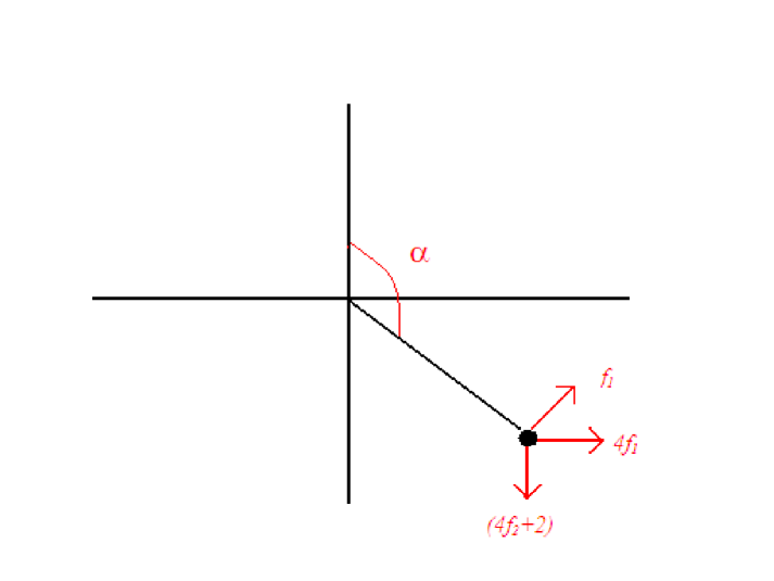
Figure 14: The Gribov pendulum

From Fig.14, we have

$$\frac{d^{2}y}{d\tau^{2}} = -(2+4f_{2})+4f_{1}\cos(\alpha-\frac{\pi}{2})+T\cos(\pi-\alpha)\;,$$ (323)

$$\frac{d^{2}x}{d\tau^{2}} = 4f_{1}-T\cos(\alpha-\frac{\pi}{2})+4f_{1}\sin(\alpha-\frac{\pi}{2})\;,$$

where $T$ stands for the tension. From

$$y = -\cos(\pi-\alpha)\;,$$ (324)

$$x = \sin(\pi-\alpha)\;,$$

we have

$$-\frac{d^{2}\cos(\pi-\alpha)}{d\tau^{2}} = -(2+4f_{2})+4f_{1}\cos(\alpha-\frac{\pi}{2})+T\cos(\pi-\alpha)\;,$$

$$\frac{d^{2}\sin(\pi-\alpha)\;}{d\tau^{2}} = 4f_{1}-T\cos(\alpha-\frac{\pi}{2})+4f_{1}\sin(\alpha-\frac{\pi}{2})\;.$$ (325)

Recalling that

$$\cos(\pi-\alpha) = -\cos\alpha\;,$$ (326)

$$\cos(\alpha-\frac{\pi}{2}) = \sin\alpha\;,$$

$$\sin(\pi-\alpha) = \sin\alpha\;,$$

$$\sin(\alpha-\frac{\pi}{2}) = -\cos\alpha\;,$$

it follows

$$\frac{d^{2}\cos\alpha}{d\tau^{2}} = -(2+4f_{2})+4f_{1}\sin\alpha-T\cos\alpha\;,$$ (327)

$$\frac{d^{2}\sin\alpha\;}{d\tau^{2}} = 4f_{1}-T\sin\alpha-4f_{1}\cos\alpha\;,$$

i.e.

$$\sin\alpha\frac{d^{2}\cos\alpha}{d\tau^{2}} = -(2+4f_{2})\sin\alpha+4f_{1}\sin^{2}\alpha-T\sin\alpha\cos\alpha\;,$$ (328)

$$\cos\alpha\frac{d^{2}\sin\alpha\;}{d\tau^{2}} = 4f_{1}\cos\alpha-T\sin\alpha\cos\alpha-4f_{1}\cos^{2}\alpha\;.$$

Eliminating the tension $T$, one gets

$$\sin\alpha\frac{d^{2}\cos\alpha}{d\tau^{2}}-\cos\alpha\frac{d^{2}\sin\alpha\;}{d\tau^{2}}=-(2+4f_{2})\sin\alpha+4f_{1}\sin^{2}\alpha-4f_{1}\cos\alpha+4f_{1}\cos^{2}\alpha\;,$$ (329)

which becomes

$$-\sin\alpha\frac{d\left(\alpha^{\prime}\sin\alpha\right)}{d\tau}-\cos\alpha\frac{d\left(\alpha^{\prime}\cos\alpha\right)\;}{d\tau}=-(2+4f_{2})\sin\alpha-4f_{1}\cos\alpha+4f_{1}\;.$$ (330)

Thus

$$\alpha^{\prime\prime}-(2+4f_{2})\sin\alpha+4f_{1}(1-\cos\alpha)=0\;.$$ (331)

Finally, adding the damping term $\alpha^{\prime}$, one gets

$$\alpha^{\prime\prime}+\alpha^{\prime}-(2+4f_{2})\sin\alpha+4f_{1}(1-\cos\alpha)=0\;,$$ (332)

which is precisely the Gribov condition $\left(\ref{eq39}\right)$.

Appendix C Appendix C. Brief introduction to homotopy and winding number

We shall give here a short introduction to the homotopy and to the winding number, following the references by S. Coleman [21] and by P. Goddard and P. Mansfield [22].

C.1 Homotopy

We shall be interested in the study of continuous mappings $\left\{\phi\right\}$ between the $n-$dimensional hyper-sphere $S^{n}$ and the coset space $\mathcal{M}=G/H$, where $G$ is a Lie group and $H$ a subgroup

$$\phi(x):S^{n}\rightarrow\mathcal{M}\;,\;\;\;x\in S^{n}$$ (333)

• Definition: Two continuous maps $\phi$, $g$ are said to be homotopic if there exists a map $F(x,t)$, with $0\leq t\leq 1$

  $$F(x,t):S^{n}\times\left[0,1\right]\rightarrow\mathcal{M\;},\;$$ (334)

  which interpolates continuously between them, namely

  $$F(x,0)=\phi\;,\;\;\;{{\mathrm{and\ \,\,\,\,\,\,}}F(x,1)=g\;\;.}$$ (335)

The existence of a homotopy between $\phi$ and $g$ will be denoted by $\phi\sim$ $g$. The set of maps $\left\{\phi:S^{n}\rightarrow\mathcal{M}\right\}$ can be divided into disjoint classes of mutually homotopic maps, the homotopy classes, denoted by $\pi_{n}(\mathcal{M})$.

C.2 The winding number

In the case in which $\mathcal{M}=S^{n}$, i.e.

$$\phi:S^{n}\rightarrow S^{n}\;,$$ (336)

it can be shown that the equivalence homotopy classes are labelled by the winding number: two maps, $\phi$, $g:S^{n}\rightarrow S^{n}$, can be continuously deformed into one another if and only if $\phi(x)$ and $g(x)\;$cover $S^{n}$ the same number of times as $x$ covers it once. Thus $\pi_{n}(S^{n})=\mathcal{Z}$, the set of all integers.

• Example 1. $g:S^{1}\rightarrow S^{1}$

  Let us consider the mapping $g(\theta):S^{1}\rightarrow S^{1}$, where $\theta\in\left[0,2\pi\right]$ and $S^{1}$ is the unit circle. For the identity map we have

  $$g^{(1)}(\theta)=e^{i\theta}=\cos\theta+i\sin\theta\;.$$ (337)

  As $\theta\in\left[0,2\pi\right]$ covers $S^{1}$, $g^{(1)}(\theta)$ covers $S^{1}$ once. The map

  $$g^{(2)}(\theta)=e^{i2\theta}=\cos 2\theta+i\sin 2\theta\;,$$ (338)

  covers $S^{1}$ twice as $\theta$ covers $S^{1}$. In general,

  $$g^{(\nu)}(\theta)=e^{i\nu\theta}=\cos\nu\theta+i\sin\nu\theta\;,$$ (339)

  with $\nu$ integer, covers $S^{1}$ $\nu-$times as $\theta$ covers $S^{1}$ once. The integer $\nu$ is called the winding number. It measures the number of times we wind around $S^{1}$ as we go once around the circle in two-space.

• The following result holds:

  Every mapping from $S^{1}\rightarrow S^{1}$ is homotopic to one of the mappings $g^{(\nu)}(\theta)$, with $\nu$ integer. From this result it follows that we can associate a winding number with every continuous mapping from $S^{1}\rightarrow S^{1}$.

The winding number can be represented by the integral

$$\nu=-\frac{i}{2\pi}\int_{0}^{2\pi}d\theta\left(g^{(\nu)}(\theta)\right)^{-1}\frac{d}{d\theta}g^{(\nu)}(\theta)\;.$$ (340)

Moreover, it can be proven that the quantity $\int_{0}^{2\pi}d\theta g^{-1}\partial_{\theta}g$ is invariant under continuous deformations, i.e. it has a topological meaning. Indeed, denoting by $\delta g=i\left(\delta\lambda\right)g$ a general infinitesimal deformation, where $\delta\lambda$ is an infinitesimal real function on the circle $S^{1}$, it follows

$$gg^{-1} = 1\;\Longrightarrow\left(\delta g\right)g^{-1}=-g\left(\delta g^{-1}\right)\;,$$ (341)

$$\delta g^{-1} = -g^{-1}\left(\delta g\right)g^{-1}\;=-ig^{-1}\delta\lambda\;.$$

Thus

$$\delta\int_{0}^{2\pi}d\theta g^{-1}\partial_{\theta}g = \int_{0}^{2\pi}d\theta\left(-ig^{-1}\delta\lambda\partial_{\theta}g+ig^{-1}\left(\partial_{\theta}\delta\lambda\right)g+ig^{-1}\delta\lambda\partial_{\theta}g\right)$$ (342)

$$= i\int_{0}^{2\pi}d\theta\partial_{\theta}\delta\lambda=0\;.$$

Also, if

$$g(\theta)=g^{(\nu_{1})}(\theta)g^{(\nu_{2})}(\theta)\;,$$ (343)

it follows that

$$\nu=\nu_{1}+\nu_{2}\;.$$ (344)

• Example 2. $g:S^{3}\rightarrow SU(2)$

  Let us discuss now the homotopy between the three-dimensional hyper-sphere $S^{3}$ and the group $SU(2)$

  $$g:S^{3}\rightarrow SU(2)\;.$$ (345)

  The unit hyper-sphere $S^{3}$ can be parametrized by local coordinates $x_{\mu},\;\mu=1,2,3,4,\;x_{\mu}x_{\mu}=1$. We may also choose three angles $\left\{\theta_{1},\;\theta_{2},\;\theta_{3}\right\}$ to parametrize $S^{3}$. The group $SU(2)$ is the group of unitary unimodular two by two matrices. Any such matrix can be written as

  $$g=aI+i\overrightarrow{b}\cdot\overrightarrow{\sigma}\;,$$ (346)

  where $a,\overrightarrow{b}$ are real parameters and $I$, $\overrightarrow{\sigma}$are the unit and the Pauli matrices, respectively. From

  $$\sigma_{1}=\left(\begin{array}[]{ll}0&1\\ 1&0\end{array}\right),\;\;\;\;\sigma_{2}=\left(\begin{array}[]{ll}0&i\\ -i&0\end{array}\right),\;\;\;\;\sigma_{3}=\left(\begin{array}[]{ll}1&0\\ 0&-1\end{array}\right)\;.$$ (347)

  it turns out

  $$g=\left(\begin{array}[]{ll}a+ib_{3}&b_{2}+ib_{1}\\ -b_{2}+ib_{1}&a-ib_{3}\end{array}\right)\;,$$ (348)

  so that the condition $\det g=1$ gives

  $$\det g=1\Longrightarrow a^{2}+\overrightarrow{b}\cdot\overrightarrow{b}=1\;.$$ (349)

  Thus $SU(2)$ has the topology of the sphere $S^{3}$. Therefore, the mapping $\left(\ref{c13}\right)$ becomes a mapping between two hyper-spheres $S^{3}$

  $$g:S^{3}\rightarrow S^{3}\;,$$ (350)

  the homotopy classes being classified by the winding number $\pi_{3}(S^{3})=\mathcal{Z}$. Examples of the mapping $g:S^{3}\rightarrow S^{3}$ are given by

  $$g^{(0)}(x) = 1\;,\;\;\mathrm{trivial\;mapping}\;\nu=0\;,$$ (351)

  $$g^{(1)}(x) = x_{4}I+i\overrightarrow{x}\cdot\overrightarrow{\sigma}\;\;,\;\;\;\mathrm{identity\;mapping}\;\nu=1\;,$$

  $$g^{(\nu)}(x) = \left(g^{(1)}(x)\right)^{\nu},\;\;\nu\mathrm{{\ }\mathrm{integer}{,\ }\mathrm{\;winding}\;\nu\;.}$$

• The following results hold:

• Result 1. Every mapping from $S^{3}$ to $S^{3}$ is homotopic to one of the mapping $g^{(\nu)}(x)$ of equation $\left(\ref{c19}\right)$.

• Result 2 (R. Bott). Let $G$ be a simple Lie group. Any continuous mapping from $S^{3}$ to $G$ can be continuously deformed into a mapping of $S^{3}$ into an $SU(2)$ subgroup of $G$. Thus, everything that can be established for $SU(2)$ is true for an arbitrary simple Lie group, in particular for $SU(N)$.

In the case of the mapping $g:S^{3}\rightarrow S^{3}$, the expression $\left(\ref{c8}\right)$ for the winding number generalizes to

$$\nu=\frac{1}{24\pi^{2}}Tr\int_{S^{3}}dS_{\mu}\varepsilon_{\mu\nu\rho\sigma}\left(g^{-1}\frac{\partial}{\partial x_{\nu}}g\right)\left(g^{-1}\frac{\partial}{\partial x_{\rho}}g\right)\left(g^{-1}\frac{\partial}{\partial x_{\sigma}}g\right)\;,$$ (352)

where $dS_{\mu}$ stands for the surface element of $S^{3}$. This expression can also be rewritten as

$$\nu=\frac{1}{24\pi^{2}}Tr\int_{S^{3}}d\theta_{1}d\theta_{2}d\theta_{3}\varepsilon_{ijk}\left(g^{-1}\frac{\partial}{\partial\theta_{i}}g\right)\left(g^{-1}\frac{\partial}{\partial\theta_{j}}g\right)\left(g^{-1}\frac{\partial}{\partial\theta_{k}}g\right)\;.$$ (353)

C.3 Application: Instantons in Euclidean Yang-Mills theories

As an application of the homotopy and of the winding number, let us discuss here the instanton solution of Euclidean Yang-Mills theories. Instantons are classical solutions of the equations of motion of pure Euclidean Yang-Mills theories which have finite action. Let $\left\{T^{a}\right\}$ be the anti-hermitian generators of a Lie group $G$,

$$\left[T^{a},T^{b}\right]=f^{abc}T^{c}\;.$$ (354)

Following Coleman [21], the Cartan inner product is defined by

$$\left(T^{a},T^{b}\right)=\delta^{ab}\;.$$ (355)

For instance, in the case of $SU(2)$, which we shall take as gauge group $G$, we have

$$T^{a} = -\frac{i}{2}\sigma^{a}\;,\;\;\;\;Tr\left(T^{a}T^{b}\right)=-\frac{1}{2}\delta^{ab}\;,$$ (356)

$$\left[T^{a},T^{b}\right] = -\frac{1}{4}\left[\sigma^{a},\sigma^{b}\right]=-\frac{i}{2}\varepsilon^{abc}\sigma^{c}=\varepsilon^{abc}T^{c}\;.$$

Thus

$$\left(T^{a},T^{b}\right)=-2Tr\left(T^{a}T^{b}\right)\;.$$ (357)

Let us start with the Yang-Mills Euclidean action

$$S_{YM}=\frac{1}{4g^{2}}\int{d^{4}x}\left(F_{\mu\nu},F_{\mu\nu}\right)\;,$$ (358)

with

$$F_{\mu\nu}(A)=\partial_{\mu}A_{\nu}-\partial_{\nu}{A}_{\mu}+\left[A_{\mu},A_{\nu}\right]\;.$$ (359)

The classical equations of motion are

$$D_{\mu}F_{\mu\nu}=\partial_{\mu}F_{\mu\nu}+\left[A_{\mu},F_{\mu\nu}\right]=0\;.$$ (360)

In order to have finite action, and recalling that ${d^{4}x=d\Omega}_{4}r^{3}dr$, one requires that $F_{\mu\nu}$ falls off faster than $1/r^{3}$ when $r\rightarrow\infty$, namely

$$F_{\mu\nu}\sim 1/r^{3}\;\;\;\mathrm{for}\;\;\;r\rightarrow\infty\;.$$ (361)

This condition implies that, when $r\rightarrow\infty$

$$A_{\mu}=g^{-1}\partial_{\mu}g+O(1/r^{2})\;\;\;\;\mathrm{for\;\;\;}r\rightarrow\infty\;.$$ (362)

Notice that, for a pure gauge configuration, $A_{\mu}=g^{-1}\partial_{\mu}g$, one has

$$F_{\mu\nu}(g^{-1}\partial g)=0\;.$$

In fact

$$F_{\mu\nu}(g^{-1}\partial g) = \partial_{\mu}(g^{-1}\partial_{\nu}g)-\partial_{\nu}(g^{-1}\partial_{\mu}g)+\left[(g^{-1}\partial_{\mu}g),(g^{-1}\partial_{\nu}g)\right]$$ (363)

$$= \left(\partial_{\mu}g^{-1}\right)\partial_{\nu}g+g^{-1}\partial_{\mu}\partial_{\nu}g-\left(\partial_{\nu}g^{-1}\right)\partial_{\mu}g-g^{-1}\partial_{\nu}\partial_{\mu}g$$

$$+g^{-1}\left(\partial_{\mu}g\right)g^{-1}\partial_{\nu}g-g^{-1}\left(\partial_{\nu}g\right)g^{-1}\partial_{\mu}g$$

$$= \left(\partial_{\mu}g^{-1}\right)\partial_{\nu}g-\left(\partial_{\nu}g^{-1}\right)\partial_{\mu}g-\left(\partial_{\mu}g^{-1}\right)\partial_{\nu}g+\left(\partial_{\nu}g^{-1}\right)\partial_{\mu}g$$

$$= 0$$

The boundary of the four-dimensional Euclidean space-time at infinity, $r\rightarrow\infty$, is given by the three hyper-sphere $S_{\infty}^{3}$. The behavior of the gauge field $A_{\mu}$ at infinity, eq.$\left(\ref{c32}\right)$, allows to define a map between the hyper-sphere $S_{\infty}^{3}$ and $SU(2)$;

$$g(x):S_{\infty}^{3}\rightarrow SU(2)\;.$$ (364)

Since $SU(2)$ has the topology of $S^{3}$, the mapping $\left(\ref{c34}\right)$ can be characterized by the winding number $\nu$ corresponding to the homotopy $\pi_{3}(S^{3})=\mathcal{Z}$. This means that the classical solutions of the equations of motion in pure Yang-Mills with finite action can be classified by the winding number $\nu$.

In order to find classical solutions of the equations of motion, it is useful to consider the identity

$$\int{d^{4}x}\left(F_{\mu\nu}\mp^{*}F_{\mu\nu},F_{\mu\nu}\mp^{*}F_{\mu\nu}\right)\geq 0\;,$$ (365)

where ${}^{*}F_{\mu\nu}$ is the dual of $F_{\mu\nu}$

$${}^{\ast}F_{\mu\nu} = \frac{1}{2}\varepsilon_{\mu\nu\rho\sigma}F_{\rho\sigma}\;,$$ (366)

$$\varepsilon_{\mu\nu\rho\sigma}\varepsilon_{\mu\nu\lambda\delta} = 2\left(\delta_{\rho\lambda}\delta_{\sigma\delta}-\delta_{\rho\delta}\delta_{\sigma\lambda}\right)\;.$$

From eq.$\left(\ref{c35}\right)$ we have

$$\int{d^{4}x}\left(F_{\mu\nu}\mp^{*}F_{\mu\nu},F_{\mu\nu}\mp^{*}F_{\mu\nu}\right)=\int{d^{4}x}\left(\left(F_{\mu\nu},F_{\mu\nu}\right)+\left({}^{*}F_{\mu\nu},^{*}F_{\mu\nu}\right)\mp 2\left(F_{\mu\nu},^{*}F_{\mu\nu}\right)\right)$$ (367)

Since ${}^{*}\left({}^{*}F_{\mu\nu}\right)=F_{\mu\nu}$, it follows

$$\frac{1}{4g^{2}}\int{d^{4}x}\left(F_{\mu\nu},F_{\mu\nu}\right)\geq\frac{1}{4g^{2}}\left|\int{d^{4}x}\left(F_{\mu\nu},^{*}F_{\mu\nu}\right)\right|$$ (368)

The bound $\left(\ref{c38}\right)$ is saturated when

$$F_{\mu\nu}=\pm^{*}F_{\mu\nu}=\pm\frac{1}{2}\varepsilon_{\mu\nu\rho\sigma}F_{\rho\sigma}\;.$$ (369)

This condition is a first order differential equation. The solutions to the self-dual equation

$$F_{\mu\nu}=^{*}F_{\mu\nu}=\frac{1}{2}\varepsilon_{\mu\nu\rho\sigma}F_{\rho\sigma}\;,\;$$ (370)

are called instantons (anti-instantons are solutions of $F_{\mu\nu}=-^{*}F_{\mu\nu}$). Thus, for an instanton, we have the equality

$$\frac{1}{4g^{2}}\int{d^{4}x}\left(F_{\mu\nu},F_{\mu\nu}\right)=\frac{1}{4g^{2}}\left|\int{d^{4}x}\left(F_{\mu\nu},^{*}F_{\mu\nu}\right)\right|\;.$$ (371)

• It is useful to observe that, from the self-dual condition, $F_{\mu\nu}=^{*}F_{\mu\nu}$, one has

  $$D_{\mu}F_{\mu\nu}=\frac{1}{2}\varepsilon_{\mu\nu\rho\sigma}D_{\mu}F_{\rho\sigma}=0\;,$$ (372)

  due to the Bianchi identity. This means that instantons are solutions of the equations of motion of pure Euclidean Yang-Mills theories.

• Another important property of the instantons is that they give vanishing contribution to the energy-momentum tensor $\Theta_{\mu\nu}$, as it is apparent from

  $$\Theta_{\mu\nu}=\frac{1}{2g^{2}}\left(F_{\mu\rho}^{a}+^{*}F_{\mu\rho}^{a}\right)\left(F_{\nu\rho}^{a}-^{*}F_{\nu\rho}^{a}\right)\;,$$ (373)

It is useful to show now that the quantity $\int{d^{4}x}\left(F_{\mu\nu},^{*}F_{\mu\nu}\right)=\int{d^{4}x}\left(F_{\mu\nu}^{a}{}^{*}F_{\mu\nu}^{a}\right)$ is directly related to the winding number $\nu$. In order to establish the relationship between $\int{d^{4}x}\left(F_{\mu\nu},^{*}F_{\mu\nu}\right)$ and $\nu$, let us first prove the identity

$$Tr\left(F_{\mu\nu}{}^{*}F_{\mu\nu}\right) = \partial_{\mu}\mathcal{G}_{\mu}\;,$$ (374)

$$\mathcal{G}_{\mu} = Tr\varepsilon_{\mu\nu\rho\sigma}\left(A_{\nu}F_{\rho\sigma}-\frac{2}{3}A_{\nu}A_{\rho}A_{\sigma}\right)\;.$$

Making use of the Bianchi identity, $\varepsilon_{\mu\nu\rho\sigma}D_{\mu}F_{\rho\sigma}=0$, we have

$$\partial_{\mu}\mathcal{G}_{\mu} = Tr\varepsilon_{\mu\nu\rho\sigma}\partial_{\mu}\left(A_{\nu}F_{\rho\sigma}-\frac{2}{3}A_{\nu}A_{\rho}A_{\sigma}\right)$$

$$= Tr\varepsilon_{\mu\nu\rho\sigma}\left(\left(\partial_{\mu}A_{\nu}\right)F_{\rho\sigma}+A_{\nu}\partial_{\mu}F_{\rho\sigma}-2\left(\partial_{\mu}A_{\nu}\right)A_{\rho}A_{\sigma}\right)$$

$$= Tr\varepsilon_{\mu\nu\rho\sigma}\left(\frac{1}{2}\left(\partial_{\mu}A_{\nu}-\partial_{\nu}A_{\mu}\right)F_{\rho\sigma}-A_{\nu}\left[A_{\mu},F_{\rho\sigma}\right]-\left(\partial_{\mu}A_{\nu}-\partial_{\nu}A_{\mu}\right)A_{\rho}A_{\sigma}\right)\;$$

$$= Tr\varepsilon_{\mu\nu\rho\sigma}\left(\frac{1}{2}F_{\mu\nu}F_{\rho\sigma}-\frac{1}{2}\left[A_{\mu},A_{\nu}\right]F_{\rho\sigma}-A_{\nu}A_{\mu}F_{\rho\sigma}+A_{\nu}F_{\rho\sigma}A_{\mu}-F_{\mu\nu}A_{\rho}A_{\sigma}\right)$$

$$+Tr\varepsilon_{\mu\nu\rho\sigma}\left(\left[A_{\mu},A_{\nu}\right]A_{\rho}A_{\sigma}\right)$$

$$= Tr\varepsilon_{\mu\nu\rho\sigma}\left(\frac{1}{2}F_{\mu\nu}F_{\rho\sigma}-A_{\mu}A_{\nu}F_{\rho\sigma}+A_{\mu}A_{\nu}F_{\rho\sigma}+A_{\mu}A_{\nu}F_{\rho\sigma}-A_{\rho}A_{\sigma}F_{\mu\nu}\right)$$

$$+Tr\varepsilon_{\mu\nu\rho\sigma}\left(\left[A_{\mu},A_{\nu}\right]A_{\rho}A_{\sigma}\right)$$

$$= Tr\varepsilon_{\mu\nu\rho\sigma}\left(\frac{1}{2}F_{\mu\nu}F_{\rho\sigma}+\left[A_{\mu},A_{\nu}\right]A_{\rho}A_{\sigma}\right)\;.$$

The term $Tr\varepsilon_{\mu\nu\rho\sigma}\left[A_{\mu},A_{\nu}\right]A_{\rho}A_{\sigma}$ vanishes due to the Jacoby identity

$$Tr\varepsilon_{\mu\nu\rho\sigma}\left[A_{\mu},A_{\nu}\right]A_{\rho}A_{\sigma} = \frac{1}{2}Tr\varepsilon_{\mu\nu\rho\sigma}\left[A_{\mu},A_{\nu}\right]\left[A_{\rho},A_{\sigma}\right]$$ (376)

$$= \frac{1}{2}\varepsilon_{\mu\nu\rho\sigma}A_{\mu}^{a}A_{\nu}^{b}A_{\rho}^{c}A_{\sigma}^{d}f^{abm}f^{cdn}TrT^{m}T^{n}$$

$$= -\frac{1}{4}\varepsilon_{\mu\nu\rho\sigma}A_{\mu}^{a}A_{\nu}^{b}A_{\rho}^{c}A_{\sigma}^{d}f^{abm}f^{cdm}$$

$$= 0\;.$$

Thus, we conclude that

$$\partial_{\mu}\mathcal{G}_{\mu}=Tr\varepsilon_{\mu\nu\rho\sigma}\frac{1}{2}F_{\mu\nu}F_{\rho\sigma}=Tr\left(F_{\mu\nu}{}^{*}F_{\mu\nu}\right)\;.$$ (377)

Moreover, making use of the Stokes theorem we obtain

$$Tr\int d^{4}x\left(F_{\mu\nu}{}^{*}F_{\mu\nu}\right)=\int d^{4}x\partial_{\mu}\mathcal{G}_{\mu}=Tr\int_{S_{\infty}^{3}}dS_{\mu}\varepsilon_{\mu\nu\rho\sigma}\left(A_{\nu}F_{\rho\sigma}-\frac{2}{3}A_{\nu}A_{\rho}A_{\sigma}\right)\;.$$ (378)

For a classical solution of the equations of motion with finite action, we have that on the hyper-sphere at infinity $S_{\infty}^{3}$

$$A_{\mu} = g^{-1}\partial_{\mu}g\;\;\;\;\mathrm{on}\;\;S_{\infty}^{3}\mathrm{\;}$$ (379)

$$F_{\mu\nu} = 0\;\;\;\mathrm{on}\;\;S_{\infty}^{3}\;.$$

Therefore, for an instanton solution

$$Tr\int d^{4}x\left(F_{\mu\nu}{}^{*}F_{\mu\nu}\right) = Tr\int_{S_{\infty}^{3}}dS_{\mu}\varepsilon_{\mu\nu\rho\sigma}\left(A_{\nu}F_{\rho\sigma}-\frac{2}{3}A_{\nu}A_{\rho}A_{\sigma}\right)$$

$$= -\frac{2}{3}Tr\int_{S_{\infty}^{3}}dS_{\mu}\varepsilon_{\mu\nu\rho\sigma}\left(A_{\nu}A_{\rho}A_{\sigma}\right)$$

$$= -\frac{2}{3}Tr\int_{S_{\infty}^{3}}dS_{\mu}\varepsilon_{\mu\nu\rho\sigma}\left(g^{-1}\partial_{\nu}g\right)\left(g^{-1}\partial_{\rho}g\right)\left(g^{-1}\partial_{\sigma}g\right)$$

$$= -16\pi^{2}\nu\;,$$

namely

$$\nu=-\frac{1}{16\pi^{2}}Tr\int d^{4}x\left(F_{\mu\nu}{}^{*}F_{\mu\nu}\right)\;,$$ (381)

or

$$\nu=\frac{1}{32\pi^{2}}\int d^{4}x\left(F_{\mu\nu}{},^{*}F_{\mu\nu}\right)=\frac{1}{64\pi^{2}}\;\int d^{4}x\varepsilon_{\mu\nu\rho\sigma}F_{\mu\nu}^{a}F_{\rho\sigma}^{a}\;.$$ (382)

The expression for $\nu$, eq.$\left(\ref{c52}\right)$, is called the Pontryagin index, whilst the integrand is the Pontryagin density. Thus, for an instanton with winding number $\nu$

$$S_{YM}=\frac{1}{4g^{2}}\int{d^{4}x}F_{\mu\nu}^{a}F_{\mu\nu}^{a}=\frac{8\pi^{2}}{g^{2}}\left|\nu\right|\;.\;$$ (383)

In the case of $SU(2)$, the explicit solution for the instanton with $\nu=1$ has been given by Belavin, Polyakov, Schwartz, Tyupkin, and reads

$$A_{\mu} = f(r^{2})\left(g^{(1)}\right)^{-1}\partial_{\mu}g^{(1)}\;,$$ (384)

$$g^{(1)} = \frac{x_{4}+i\overrightarrow{x}\cdot\overrightarrow{\sigma}}{r}\;,\;\;\;\;r=\sqrt{x_{\mu}x_{\mu}}\;,$$

$$f(r^{2}) = \frac{r^{2}}{r^{2}+\rho^{2}}\;,$$

where $\rho$ is an arbitrary constant, called the size of the instanton.

Appendix D Appendix D. Polar coordinates

Let us remind here some useful relationships in polar coordinates:

$$x = r\sin\theta\cos\varphi\;,$$

$$y = r\sin\theta\sin\varphi\;,$$

$$z = r\cos\theta\;.$$ (385)

Thus, for the orthonormal basis $\left(\overrightarrow{e}_{r},\;\overrightarrow{e}_{\theta},\;\overrightarrow{e}_{\varphi}\right)$ we have

$$\overrightarrow{e}_{r} = \sin\theta\cos\varphi\overrightarrow{e}_{x}+\sin\theta\sin\varphi\overrightarrow{e}_{y}+\cos\theta\overrightarrow{e}_{z}\;,$$ (386)

$$\overrightarrow{e}_{\theta} = \cos\theta\cos\varphi\overrightarrow{e}_{x}+\cos\theta\sin\varphi\overrightarrow{e}_{y}-\sin\theta\overrightarrow{e}_{z}\;,$$

$$\overrightarrow{e}_{\varphi} = \overrightarrow{e}_{r}\times\overrightarrow{e}_{\theta}=-\sin\varphi\overrightarrow{e}_{x}+\cos\varphi\overrightarrow{e}_{y}\;.$$

Let $\overrightarrow{v}$ be a vector. We have

$$\overrightarrow{v}=v_{x}\overrightarrow{e}_{x}+v_{y}\overrightarrow{e}_{y}+v_{z}\overrightarrow{e}_{z}\;=v_{r}\overrightarrow{e}_{r}+v_{\theta}\overrightarrow{e}_{\theta}+v_{\varphi}\overrightarrow{e}_{\varphi}\;,\;$$ (387)

with

$$v_{r} = \overrightarrow{v}\cdot\overrightarrow{e}_{r}=v_{x}\sin\theta\cos\varphi+v_{y}\sin\theta\sin\varphi+v_{z}\cos\theta\;,$$

$$v_{\theta} = \overrightarrow{v}\cdot\overrightarrow{e}_{\theta}=v_{x}\cos\theta\cos\varphi+v_{y}\cos\theta\sin\varphi-v_{z}\sin\theta\;,$$

$$v_{\varphi} = \overrightarrow{v}\cdot\overrightarrow{e}_{\varphi}=-v_{x}\sin\varphi+v_{y}\cos\varphi\;.$$ (388)

Also,

$$\overrightarrow{\nabla}f = \frac{\partial f}{\partial r}\overrightarrow{e}_{r}+\frac{1}{r}\frac{\partial f}{\partial\theta}\overrightarrow{e}_{\theta}+\frac{1}{r\sin\theta}\frac{\partial f}{\partial\varphi}\overrightarrow{e}_{\varphi}\;,$$

$$\overrightarrow{\nabla}^{2}f = \frac{1}{r^{2}}\frac{\partial}{\partial r}\left(r^{2}\frac{\partial f}{\partial r}\right)+\frac{1}{r^{2}\sin\theta}\frac{\partial}{\partial\theta}\left(\sin\theta\frac{\partial f}{\partial\theta}\right)+\frac{1}{r^{2}\sin^{2}\theta}\frac{\partial^{2}f}{\partial\varphi^{2}}\;,$$

$$\overrightarrow{\nabla}\cdot\overrightarrow{v} = \frac{1}{r^{2}}\frac{\partial\left(r^{2}v_{r}\right)}{\partial r}+\frac{1}{r\sin\theta}\frac{\partial\left(\sin\theta v_{\theta}\right)}{\partial\theta}+\frac{1}{r\sin\theta}\frac{\partial v_{\varphi}}{\partial\varphi}\;.$$ (389)