A transition in the spectrum of the topological sector of $\phi_{2}^{4}$ theory at strong coupling

Abstract

We investigate the strong coupling region of the topological sector of the two-dimensional $\phi^{4}$ theory. Using discrete light cone quantization (DLCQ), we extract the masses of the lowest few excitations and observe level crossings. To understand this phenomena, we evaluate the expectation value of the integral of the normal ordered $\phi^{2}$ operator and we extract the number density of constituents in these states. A coherent state variational calculation confirms that the number density for low-lying states above the transition coupling is dominantly that of a kink-antikink-kink state. The Fourier transform of the form factor of the lowest excitation is extracted which reveals a structure close to a kink-antikink-kink profile. Thus, we demonstrate that the structure of the lowest excitations becomes that of a kink-antikink-kink configuration at moderately strong coupling. We extract the critical coupling for the transition of the lowest state from that of a kink to a kink-antikink-kink. We interpret the transition as evidence for the onset of kink condensation which is believed to be the physical mechanism for the symmetry restoring phase transition in two-dimensional $\phi^{4}$ theory.

I Introduction

As is well known dashen ; rajaraman ; gj , topological excitations (kinks) exist in classical two-dimensional $\phi^{4}$ model with negative quadratic term (broken phase). However, the study of topological objects in quantum field theory is highly nontrivial. Most of the investigations to date use semi-classical or Hartree approximations. Using the techniques of constructive quantum field theory glimmj , it was proven rigorously that in quantum theory, a stable kink state is separated from the vacuum by a mass gap of the order $\lambda^{-1}$ and from the rest of the spectrum by an upper gap froh . More detailed nonperturbative information on the spectrum of the mass operator or on other observables from rigorous approaches is not available. It is worthwhile to recall that the study of these objects in lattice field theory is also highly non-trivial Ciria ; Ardekani . For very recent work on the kinks in two dimensional $\phi^{4}$ theory in the Hartree approximation, see Refs. bb ; salle .

Light front quantization offers many advantages for the study of two dimensional quantum field theories. As is well-known, of the three Poincare generators only the Hamiltonian is dynamical. In contrast, in the conventional instant form formulation, only momentum is a kinematical operator. Kinematical boost invariance allows for the extraction of Lorentz invariant observables such as the parton distribution function which has the simple interpretation of a number density. The formulation allows for the extraction of the spectrum of the invariant mass operator in a straight-forward manner. In this work we utilize the discrete version of the light front quantization, namely, discrete light cone quantization (DLCQ) dlcq for numerical investigations of two dimensional $\phi^{4}$ theory with anti periodic boundary condition (APBC) at strong coupling. Since the zero momentum mode is absent, the Hamiltonian has the simplest Fock space structure in this case.

The quantum kink on the light front was first addressed by Baacke Baacke in the context of semi-classical quantization. Recently Rozowsky and Thorn RT , with the help of a coherent state variational calculation, have shown that it is possible to extract the mass of topological excitations in DLCQ with periodic boundary condition (PBC) while dropping the zero momentum mode. Motivated by the remarkable work of these authors, we have initiated the study kinkplb of topological objects in the broken symmetry phase of two dimensional $\phi^{4}$ theory using APBC in DLCQ. We presented evidence for degenerate ground states, which is both a signature of spontaneous symmetry breaking and mandatory for the existence of kinks. Guided by a constrained variational calculation with a coherent state ansatz, we then extracted the vacuum energy and kink mass and compared with classical and semi-classical results. We compared the DLCQ results for the number density of partons in the kink state and the Fourier transform of the form factor of the kink with corresponding observables in the coherent variational kink state. We have also carried out similar investigations using PBC pp1 .

In this work, we probe the strong coupling region of the topological sector of the theory with topological charge $\pm 1$. The plan of this work is as follows. We follow the notations and conventions of Ref. kinkplb . Major aspects of Hamiltonian diagonalization are given in Sec. II. In Sec. III we extract of the mass of the lowest few excitations as a function of the coupling and display results for the gaps in mass-squared. As the coupling increases, we observe level crossing in the spectrum. In this section, we also discuss the manifestation of level crossing in another observable, namely, the expectation value of the integral of the normal ordered $\phi^{2}$ operator. To gain further insights, we need to probe other physical properties of the low-lying excitations. Toward this end, we perform DLCQ calculations of the parton density and the Fourier transform of the form factor of the lowest excitation at moderately strong couplings and the results are presented in Sec. IV. In the same section a coherent state variational calculation of the kink-antikink-kink profile and corresponding parton density are also given. Sec. V contains a discussion, summary and conclusions.

II Hamiltonian and Diagonalization

We start from the Lagrangian density

$${\cal L}=\frac{1}{2}\partial^{\mu}\phi\partial_{\mu}\phi+\frac{1}{2}\mu^{2}\phi^{2}-\frac{\lambda}{4!}\phi^{4}.$$ (1)

The light front variables are defined by $x^{\pm}=x^{0}\pm x^{1}$.

The Hamiltonian density

$${\cal P}^{-}=-\frac{1}{2}\mu^{2}\phi^{2}+\frac{\lambda}{4!}\phi^{4}$$ (2)

defines the Hamiltonian

$$P^{-} = \int dx^{-}{\cal P}^{-}~{}\equiv\frac{L}{2\pi}H$$ (3)

where $L$ defines our compact domain $-L\leq x^{-}\leq+L$. Throughout this work we address the energy spectrum of $H$.

The longitudinal momentum operator is

$$P^{+} = \frac{1}{2}\int_{-L}^{+L}dx^{-}\partial^{+}\phi\partial^{+}\phi\equiv\frac{2\pi}{L}K$$ (4)

where $K$ is the dimensionless longitudinal momentum operator. The mass squared operator $M^{2}=P^{+}P^{-}=KH$.

In DLCQ with APBC, the field expansion has the form

$$\Phi(x^{-})=\frac{1}{\sqrt{4\pi}}\sum_{n}\frac{1}{\sqrt{n}}\left[a_{n}e^{-i\frac{n\pi}{L}x^{-}}+a_{n}^{\dagger}e^{i\frac{n\pi}{L}x^{-}}\right].$$ (5)

Here $n=\frac{1}{2},\frac{3}{2},\ldots.$

The normal ordered Hamiltonian is given by

$$H = -\mu^{2}\sum_{n}\frac{1}{n}a_{n}^{\dagger}a_{n}+\frac{\lambda}{4\pi}\sum_{k\leq l,m\leq n}~{}\frac{1}{N_{kl}^{2}}~{}\frac{1}{N_{mn}^{2}}~{}\frac{1}{\sqrt{klmn}}a_{k}^{\dagger}a_{l}^{\dagger}a_{n}a_{m}\delta_{k+l,m+n}$$ (6)

$$+\frac{\lambda}{4\pi}\sum_{k,l\leq m\leq n}~{}\frac{1}{N_{lmn}^{2}}~{}\frac{1}{\sqrt{klmn}}~{}\left[a_{k}^{\dagger}a_{l}a_{m}a_{n}+a_{n}^{\dagger}a_{m}^{\dagger}a_{l}^{\dagger}a_{k}\right]~{}\delta_{k,l+m+n}$$

with

$$N_{lmn} = 1,~{}l\neq m\neq n,$$ (7)

$$= \sqrt{2!},~{}l=m\neq n,~{}l\neq m=n,$$

$$= \sqrt{3!},~{}l=m=n,$$

and

$$N_{kl} = 1,k\neq l,~{}$$ (8)

$$= \sqrt{2!},~{}k=l.$$

Since the Hamiltonian exhibits the $\phi\rightarrow-\phi$ symmetry, the even and odd particle sectors of the theory are decoupled. When the coefficient of $\phi^{2}$ in the Hamiltonian is positive, at weak coupling, the lowest state in the odd particle sector is a single particle carrying all the momentum. In the even particle sector, the lowest state consists of two particles having equal momentum. Thus for massive particles, there is a distinct mass gap between odd and even particle sectors. When the coefficient of $\phi^{2}$ in the Hamiltonian is negative, at weak coupling, the situation is drastically different. Now, the lowest states in the odd and even particle sectors consist of the maximum number of particles carrying the lowest allowed momentum. Thus, in the continuum limit, the possibility arises that the states in the even and odd particle sectors become degenerate. In this case, for any state $|e>$ in the even sector we find a state $|o>$ in the odd particle sector with the same mass. Hence, we can construct two degenerate states of mixed symmetry which are eigenstates of the Hamiltonian: $|\alpha>=|e>+|o>$ and $|-\alpha>=|e>-|o>$, Under $\phi$ parity $|\alpha>~{}\rightarrow~{}|-\alpha>$ and $|-\alpha>~{}\rightarrow|~{}\alpha>$. These eigenstates of the Hamiltonian do not respect the symmetry of the Hamiltonian and hence a clear signal of SSB is the degeneracy of the spectrum in the even and odd particle sectors. Recall that with APBC, for integer (half integer) $K$, we have even (odd) particle sectors. Thus at finite $K$, we can compare the spectra for an integer K value and its neighboring half integer $K$ value and look for degenerate states.

All the results presented here were obtained on clusters of computers ($\leq$ 15 processors) using the many fermion dynamics (MFD) code adapted to bosons mfd . The Lanczos diagonalization method is used in a highly scalable algorithm that allows us to proceed to high enough values of $K$ for smooth $K\rightarrow\infty$ extrapolations. For our largest value, $K=60$, the Hamiltonian matrix reaches the dimensionality 1,928,175, with configurations up to 120 bosons participating.

III Level crossing in the spectrum at strong coupling

In Ref. kinkplb we presented the lowest four eigenvalues as a function of $\frac{1}{K}$ for $\lambda=1.0$ and the extracted values of the vacuum energy density and kink mass. We saw that the values extracted are close to the semi-classical result.

As we increase the coupling, we find that the lowest two energy levels cross each other. The value of the coupling at which this occurs lowers as $K$ increases. In Fig. 1(a), we present the mass squared differences for the lowest five excitations as a function of $\lambda$ in the critical region for the even ($K=55$) particle sector. Many interesting features are exhibited in this figure. Not only the lowest two levels but all the low-lying levels cross. Before the occurrence of level crossing, the nature of the spectrum is as follows. There is a substantial size to the mass-squared gap between the lowest three excitations. Thereafter, the gaps become more closely packed, and more evenly spread.

In the semi-classical analysis rajaraman , the lowest states, in order of excitation, are kink, excited kink, kink plus boson, and the continuum states. The wide gaps that exist between the second and first level and the third and first level and the close packing of higher levels are consistent with the expectations from semi-classical analysis. But as we see in Fig. 1(a), the gaps vanish at strong coupling. After the level crossings, we observe almost equally spaced gaps for the mass-squared of all the low-lying excitations suggestive of a harmonic mass-squared spectrum. This indicates that the nature of low lying levels are substantially different in the two regions of the coupling.

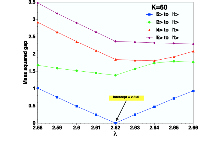
Figure 2: (Color online) Same as in Fig. 1 but for $K=60$. The upper gaps are connected by straight line segments while the straight lines of the lowest gaps are obtained as in Fig. 1(b).

In Figs. 1(b), and 2 we exhibit the finer details of level crossing for $K=55$ and $60$. Here the linearity of the disappearing mass-squared gap is clearly observed. At low $K$ values, we see evidence for the mixing of lowest levels (not shown in the figures) but that mixing disappears with increasing $K$. The vanishing of the mass-squared gap is exhibited more clearly in Fig. 2. In this case we have observed vanishing mass-squared gap to a very high precision (6 significant figures) which is of the same order as the machine accuracy in single precision. i.e., there is no mixing or the level of mixing present is at or below the level of computational noise.

Another manifestation of the level crossing phenomena is found in the expectation value of the integral of the normal ordered $\phi^{2}$ operator. In Fig. 3 we show the behavior of this observable for the lowest excitation as a function of $\lambda$ for different values of $K$. The sudden drops match with level crossing points of the lowest state in the mass-squared gap spectra. For comparison we have also shown the behavior of $\phi_{classical}^{2}=6\frac{\mu^{2}}{\lambda}$ as a function of $\lambda$ in the same figure. Note that the value of $\lambda$ at which the drop occurs, $\lambda_{c}$, decreases with increasing $K$. Furthermore, we observe that as $K$ increases the difference in the $\lambda_{c}$ extracted from the even and the odd sector transitions, systematically tends towards zero. The drop in the $\phi^{2}$ observable sharpens as a function of $\lambda$ with increasing $K$. Again, this agrees well with a sharpening of level crossing with increasing $K$. As discussed in next section, the reason for this drop is the transition of the lowest states of the system from a kink type to a dominant kink-antikink-kink type. We will show that in the number density, this transition manifests as a shift of maximal occupation from the lowest momentum mode to the next available mode.

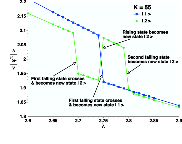
Figure 4: (Color online) $\langle\mid\phi^{2}\mid\rangle$ (see caption to Fig. 3 for the notation) as a function of $\lambda$ for $K$=55 for the lowest two excitations.

In Fig. 4 we compare the behavior of the same observable for the lowest two states for the even ($K=55$) particle sector. As one approaches the critical coupling, a set of states which are highly excited states at weak coupling drop rapidly into the low-energy region. Between the values of the coupling, 2.65 and 2.7 the first falling state crosses and becomes the new second state. In the vicinity of the coupling 2.75, the first falling state crosses and becomes the new lowest state and the rising state becomes the newest second state. Close the coupling 2.8, the second falling state becomes the new second state.

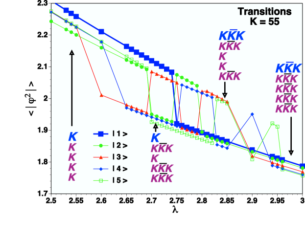
Figure 5: (Color online) $\langle\mid\phi^{2}\mid\rangle$ (see caption to Fig. 3 for the notation) as a function of $\lambda$ for $K$=55 for the lowest five excitations. The pattern of transitions correspond to 5 states falling with increasing $\lambda$ and crossing the 5 lowest states, thus replacing them and becoming the new 5 lowest states. At selected values of $\lambda$, the character of the lowest states is indicated on the figure with the top level of each column signifying the nature of the lowest state. Successive excited states are signified by the labels proceeding down the column. The letter $``$K” repesents $``$kink” while $``K{\bar{K}}K$” represents $``$kink-antikink-kink”.

In Fig. 5 we demonstrate that such level crossings occur for all the low-lying excitations. For example, at the coupling of 2.5 all the lowest five excitations are of the kink type. At the coupling of 3, all of them have become dominantly kink-antikink-kink type. It is remarkable that in the entire region of the coupling, the $\phi^{2}$ observable for all the low lying states cluster around that of either a kink or a dominantly kink-antikink-kink type. i.e., we observe no case caught in the midst of a transition. We conclude there is essentially no mixing of the lowest five states of one type with any states of the other type within numerical precision.

All these features in our results suggest we are observing the characteristics of a phase transition that can manifest in a system with a finite degrees of freedom.

IV Calculation of other observables

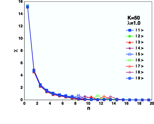
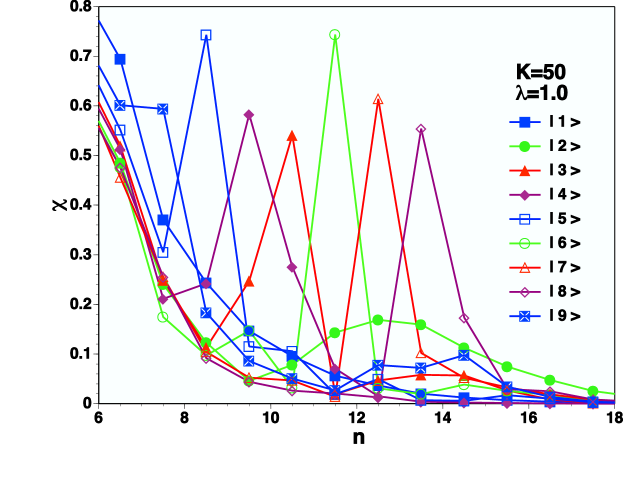
Figure 6: (Color online) (a) $\chi$ versus $n$, the half-odd integer representing light front momentum with APBC, for the lowest nine excitations for $K=50,~{}\lambda=1$. (b) Same as in (a) but showing the region from $n=6$ to $18$ in detail.

To gain further understanding of the nature of the levels that cross, we next examine the behavior of the parton density $\chi(n)$ for the lowest excitation for different values of coupling. In Figs. 6(a) and 6(b) we present the parton distribution function $\chi(n)$ for the lowest nine excitations at $\lambda=1$ and $K=50$. At small coupling, the lowest excitation is a kink state which yields a characteristic parton distribution which peaks at the lowest momentum mode available. In the semi-classical picture, the next excitation is an excited kink for which also we expect and find a smooth distribution function. The excited kink, the second excitation in the spectrum, features a broad and smooth peak spanning $n=10.5$ to $n=17.5$ as is seen in Fig. 6(b). The integrated momentum fraction under this peak accounts for 22% of the momentum sum rule.

The third and higher excitations are expected to be kink plus boson states. The characteristic peaks in Fig. 6(b) for states 3-8 are observed at $n=(10.5,9.5,8.5,11.5,12.5$ and $13.5)$ respectively. Sharp peaks suggest a boson in a pure momentum state coupling weakly to the kink. This picture is supported by the momentum fraction of approximately 20% of the sum rule carried in each of these peaks, which corresponds well to a boson positioned around n=10 in a state carrying a total light-front momentum of $K=50$.

The ninth state in the spectrum does not exhibit the simple isolated boson plus kink features and this state may indicate the onset of more complicated multi-boson excitations. It would be necessary to perform calculations at higher $K$ and for more states to further explore the higher lying features of the spectrum at this coupling.

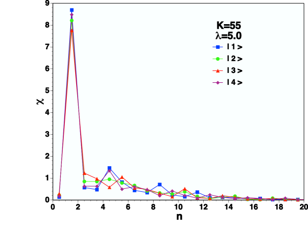
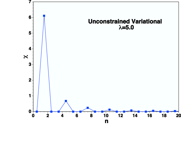
Figure 7: (Color online) (a) $\chi$ versus $n$, the half-odd integer representing light front momentum with APBC, for the lowest four excitations for $K=55,~{}\lambda=5$. (b) Kink-antikink-kink parton density in unconstrained variational calculation for $\lambda$=5.

At strong coupling the situation changes drastically. As seen from Fig. 7 (a), at $\lambda=5(K=55)$, the lowest momentum mode ($n=0.5$) for all the lowest four excitations has almost zero occupation and the next mode ($n=1.5$) has maximum occupation for all four lowest excitations. Thus, between $\lambda=1$ and $\lambda=5$, a change in the structure of the lowest excitations (kink) takes place for this $K$ value. Can one gain a better understanding of the parton structure of these states, in particular the striking feature of the absence of the lowest momentum mode? In the next subsection we carry out a coherent state variational calculation for a kink-antikink-kink state and from the calculation of the number density confirm that the lowest excitation after the first level crossing indeed corresponds dominantly to that of the kink-antikink-kink state.

IV.1 Coherent state variational calculation of kink-antikink-kink state

We have seen that a simple way to realize the parton picture of the classical kink solution in DLCQ is the unconstrained coherent state variational calculationRT . Can one understand the parton structure of other topological excitations in the same method? In particular, we are interested in the kink-antikink-kink state. (For a detailed investigation of kink-antikink-kink dynamics in classical two dimensional $\phi^{4}$ theory see Ref. mm .)

Choose as a trial state, the coherent state

$$\mid\alpha\rangle={\cal N}e^{\sum_{n}\alpha_{n}a_{n}^{\dagger}}\mid 0\rangle$$ (9)

where ${\cal N}$ is an arbitrary normalization factor.

With APBC we have

$$\frac{\langle\alpha\mid\phi(x^{-})\mid\alpha\rangle}{\langle\alpha\mid\alpha\rangle}=\frac{1}{\sqrt{4\pi}}~{}f(x^{-})$$ (10)

with

$$f(x^{-})=\sum_{n}\frac{1}{\sqrt{n}}\Big{[}\alpha_{n}e^{-i\frac{\pi}{L}nx^{-}}+\alpha_{n}^{*}e^{i\frac{\pi}{L}nx^{-}}\Big{]}~{}$$ (11)

with $n=\frac{1}{2},\frac{3}{2},...$ . Minimizing the expectation value of the Hamiltonian, we obtain

$$f_{min}=\pm\sqrt{\frac{24\pi\mu^{2}}{\lambda}}=\pm\sqrt{\frac{3}{g}}.$$ (12)

Our starting point is the expression for the function $f(x^{-})$ given in Eq. (11). With $f_{min}=\pm\sqrt{\frac{3}{g}}$, we set

$$f(x^{-}) = +\sqrt{3/g},~{}~{}-L<x^{-}<-2L/3,$$ (13)

$$= -\sqrt{3/g},~{}~{}-2L/3<x^{-}<0,$$

$$= +\sqrt{3/g},~{}~{}0<x^{-}<2L/3,$$

$$= -\sqrt{3/g},~{}~{}2L/3<x^{-}<L.$$

This yields,

$$\alpha_{n}=\sqrt{3/g}~{}\frac{i}{\pi}~{}\frac{1}{\sqrt{n}}~{}\Big{[}1-2~{}\cos(2n\pi/3)\Big{]}.$$ (14)

Thus

$$f(x^{-})=\frac{2}{\pi}\sqrt{3/g}\sum_{n}\frac{1}{n}\Big{[}1-\cos(2n\pi/3)\Big{]}\sin(2n\pi x^{-}/L)~{}.$$ (15)

The number density of constituents, i.e., parton density in light front theory is given by

$$\chi(n)=\frac{\langle\alpha\mid a_{n}^{\dagger}a_{n}\mid\alpha\rangle}{\langle\alpha\mid\alpha\rangle}=\mid\alpha_{n}\mid^{2}~{}.$$ (16)

For $\lambda=5$, the parton density of the kink-antikink-kink state is presented in Fig. 7 (b).

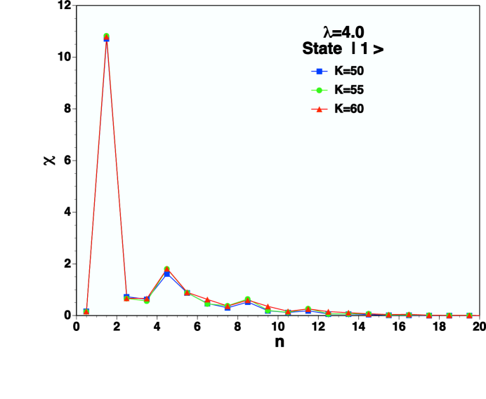
Figure 8: (Color online) $\chi$ versus $n$, the half-odd integer representing light front momentum with APBC, for the lowest excitation for $K=50,55,$ and $60$, $\lambda=4$.

In Fig. 8 we compare the number density of the lowest excitation at $\lambda=4$ for $K=50,55,60$ and show remarkable stability of results with respect to variations in $K$. Further, by comparison with the lowest state in Fig. 7(a), we see that the shape is independent of coupling and the magnitude follows the trend of the coherent state analysis.

Evaluation of the number density in the unconstrained variational calculation clearly shows that the lowest excitation after the first level crossing is definitely not a kink but a dominantly kink-antikink-kink state. It has small admixtures of other topological structures as is evident from the following. For a pure kink-antikink-kink state, $\chi(n)$ vanishes for $n=\frac{5}{2},\frac{7}{2},\frac{11}{2}$ etc as seen from Fig. 7(b) but it doesn’t vanish for these modes for the state observed after the transition as seen in Fig. 7(a). An interesting issue is whether we can identify the nature of the excitation within DLCQ, i.e., without the help from unconstrained variational calculation. This is possible since the Hamiltonian diagonalization provides us with various eigenfuctions of the lowest few excitations and we may evaluate other observables that yield more information about the structure of these states.

IV.2 Fourier transform of the form factor

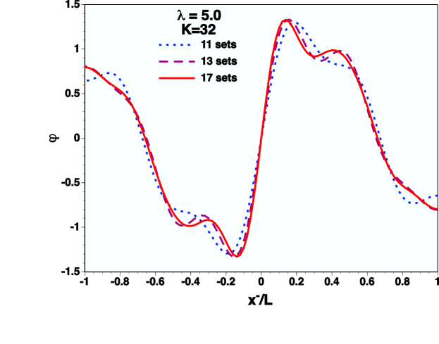
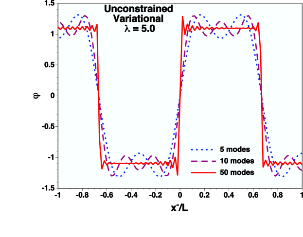
Figure 9: (Color online) (a) Fourier Transform of the kink form factor at $\lambda$=5, $K=32$. The figure legend indicates the number of adjoining momentum transfer terms (sets) included in the summation. (b) Expectation value of the field operator in the kink-antikink-kink state in the unconstrained variational calculation for $\lambda=5.0$.

An useful observable that gives direct information on the nature of the physical state is the Fourier transform of the form factor of the lowest state, which, according to Goldstone and Jackiw gj , gives the coordinate space profile of the topological excitation. The analysis of Ref. gj was restricted to weak coupling theory, whereas, we are able to perform reliable nonperturbative calculations at strong coupling. By explicitly calculating the form factor for different momentum  transfers, we perform the Fourier transform numerically. For weak coupling, the result is presented in Ref. kinkplb which reveals a kink profile. In Fig. 9(a) we present the profile of the lowest excitation in DLCQ for $\lambda=5$ and $K=32$. Results are presented for three cases where the magnitude of the maximum momentum transfer included in the sum for the Fourier transform ranges from 5 to 8. The profile is that of a dominant kink-antikink-kink state. But as we have learned from the evaluation of the number density, the state after the transition is not a pure kink-antikink-kink configuration. The appearance of more structures near the origin in Fig. 9(a) may be a consequence of this fact. In Fig. 9 (b) we present the expectation value of the field operator in the kink-antikink-kink state in the unconstrained coherent state variational calculation. It is worthwhile to note that the sharp features present in the profile in the unconstrained variational calculation as the number of modes included increases as shown in Fig. 9(b) is an artefact of the unconsrtained variational calculation which yields an infinite value for the expectation value of $K$. We expect much smoother behaviour for the constrained variational calculation which yields finite expectation value of $K$ kinkplb . Noting the close similarities of the observables in Fig. 7 (a) and (b) and Fig. 9 (a) and (b) we conclude that at a critical coupling, the lowest excitation in the topological sector with charge $\pm 1$ of broken phase of $\phi_{2}^{4}$ theory changes its character from a kink state to a state dominated by kink-antikink-kink structure.

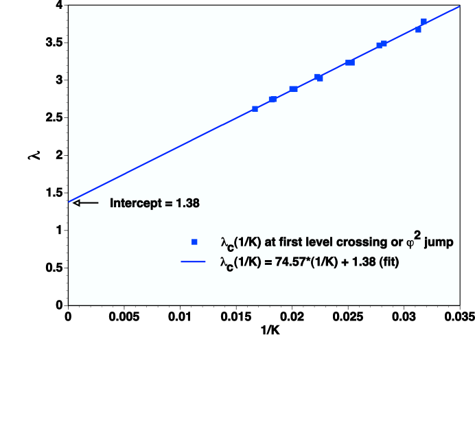
Figure 10: Critical coupling for level crossing as a function of $\frac{1}{K}$, and an indication of the critical coupling in the continuum limit.

In Fig. 10 we present the behavior of this critical coupling with $\frac{1}{K}$ from the analysis of vanishing mass-squared gaps and $\phi^{2}$ jumps as shown in Figs. 1 and 3 and extract its value in the continuum limit as $\lambda_{c}=1.38$.

We have already observed that the mass-squared gap vanishes linearly at the critical coupling for level crossing. This implies that, parameterizing the behavior of the mass-squared gap near the critical coupling as $\delta M^{2}\approx(\lambda_{c}-\lambda)^{\nu}$, we have obtained the exponent $\nu=1.0$.

V Discussion, Summary and Conclusions

To investigate the strong coupling region of the topological sector of two dimensional $\phi^{4}$ theory we have utilized DLCQ which provides us with all the advantages of the Hamiltonian approach with additional features of light front quantization.. A major bonus of using DLCQ is the detailed information we gain about the parton structure of the states. We have shown that between $\lambda=1$ and $\lambda=2$, level crossings occur in the continuum limit. The important issues to resolve are the nature of this transition and its physical implications. To settle this issue we have studied the expectation value of the integral of the normal ordered $\phi^{2}$ operator in the lowest excitations of the system. We have observed a sharp drop in this observable. We also observed a corresponding change in behavior of the number density in the lowest excitations, namely, the shift of the maximum occupation from the lowest momentum mode to the next higher momentum mode.

In the weak coupling region, one can use analytical variational calculations with a coherent state ansatz for the lowest state to gain physical insights for the DLCQ data. Following Rozowsky and Thorn RT we have carried out unconstrained variational calculations but with APBC. Variational calculations predict maximum occupation in the lowest momentum mode for the lowest eigenstate. Our numerical results show that this simple semi-classical picture becomes invalid as the coupling grows greater than 1. A coherent state variational calculation corresponding to kink-antikink-kink state predicts maximum occupation for the next higher momentum mode and almost zero occupation of the lowest momentum mode. This is consistent with the observed properties of our states above the transition.

In Ref. kinkplb , following Goldstone and Jackiw, we have calculated the Fourier transform of the form factor of the kink state in DLCQ at weak coupling and demonstrated consistency with the classical solution. At strong coupling after the drop in the $\phi^{2}$ observable, we have shown here that the profile calculated in DLCQ is approximately that of a kink-antikink-kink state. From the analysis of vanishing mass-squared gap and the drop in the $\phi^{2}$ observable we have extracted the critical coupling for the first transition in the infinite volume limit as $\lambda_{c}=1.38$.

The transition that we have observed is very sensitive to the boundary conditions. We have observed that in similar calculations performed with PBC such a transition is absent at the same value of $\lambda$. With PBC, we do observe level crossings at much higher coupling which appears to correspond to the transition from a kink-antikink state to a mixture of states with a dominant kink-antikink-kink-antikink component.

In the two-dimensional Ising model it is well-known that the physical mechanism for the symmetry restoring phase transition is the phenomena of kink condensation sf ; kogut . It is known that at strong coupling, the $\phi_{2}^{4}$ theory undergoes a symmetry restoring phase transition. As far as we know, the physical mechanism behind the phase transition has not been investigated before in the two dimensional $\phi_{2}^{4}$ quantum field theory. We have demonstrated that in this theory, at strong coupling, it is energetically favourable for a dominantly kink-antikink-kink configuration to be the lowest excitation rather than a kink configuration. At still higher coupling we have observed additional level crossings for the lowest state for both PBC and APBC. Further investigations are necessary to clarify the nature of the lowest excitation after these transitions and to quantify the critical point of the transition. In the light of all our observations, we interpret the observed level crossing presented here as the onset of kink condensation which leads to the restoration of symmetry.

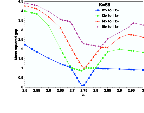
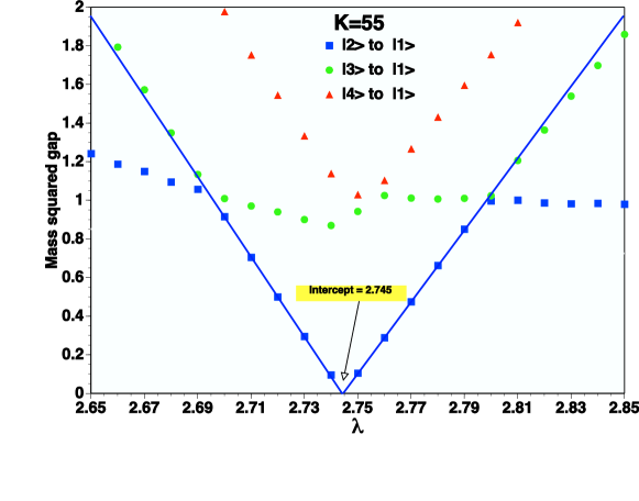
Figure 1: (Color online)(a) Mass² gap as a function of $\lambda$ for $K$=55. All calculated results are connected by straight line segments to guide the eye. (b) Same as in (a) but the detailed structure for a narrow range of $\lambda$ around the critical coupling is shown. Here, two straight lines have been fit to the lowest gap near the crossing point to extract the $``$critical” value of the coupling as indicated in the figure.

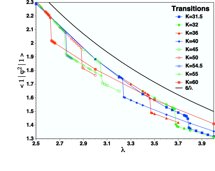
Figure 3: (Color online) $\langle 1\mid\phi^{2}\mid 1\rangle$ (short hand notation for the expectation value of the integral of the normal ordered $\phi^{2}$ operator) as a function of $\lambda$ and selected $K$ values. For comparison we have also shown $\phi_{classical}^{2}=6\frac{\mu^{2}}{\lambda}$ with $\mu^{2}=1$.

- (1) R. F. Dashen, B. Hasslacher and A. Neveu, Phys. Rev. D 10, 4130 (1974).
- (2) R. Rajaraman, An Introduction to Solitons and Instantons in Quantum Field Theory, (North-holland, Amsterdam, Netherlands, 1982).
- (3) J. Goldstone and R. Jackiw, Phys. Rev. D 11, 1486 (1975).
- (4) J. Glimm and A. Jaffe, Quantum Physics: A Functional Integral Point of View, (Springer, New York, 1981).
- (5) J. Bèllissard, J. Frohlich and B. Gidas, Phys. Rev. Lett. 38, 619 (1977); J. Frohlich and P. Marchetti, Comm. Math. Phys. 116, 127 (1988).
- (6) J. C. Ciria and A. Tarancon, Phys. Rev. D 49, 1020 (1994) [arXiv:hep-lat/9309019].
- (7) A. Ardekani and A. G. Williams, Austral. J. Phys. 52, 929 (1999) [arXiv:hep-lat/9811002].
- (8) Y. Bergner and L. M. Bettencourt, Phys. Rev. D 69, 045002 (2004); arXiv:hep-th/0305190.
- (9) M. Salle, Phys. Rev. D 69, 025005 (2004); arXiv:hep-ph/0307080.
- (10) T. Maskawa and K. Yamawaki, Prog. Theor. Phys. 56, 270 (1976); A. Casher, Phys. Rev. D 14, 452 (1976); C. B. Thorn, Phys. Rev. D 17, 1073 (1978); H.C. Pauli and S.J. Brodsky, Phys. Rev. D 32, 1993, (1985); ibid., 2001 (1985). For a review, see, S. J. Brodsky, H. C. Pauli and S. S. Pinsky, Phys. Rep. 301, 299 (1998).
- (11) J. Baacke, Z. Phys. C 1, 349 (1979).
- (12) J. S. Rozowsky and C. B. Thorn, Phys. Rev. Lett. 85, 1614 (2000) [arXiv:hep-th/0003301].
- (13) D. Chakrabarti, A. Harindranath, L. Martinovic and J. P. Vary, Phys. Lett. B 582, 196 (2004) [arXiv:hep-th/0309263]. Please note that the factors and were inadvertently dropped from the second and third lines of Eq. (6) in this paper as a result of typographical error. The computer code that generated the results presented in the paper had the correct factors in the Hamiltonian.
- (14) D. Chakrabarti, A. Harindranath, L. Martinovic, G. B. Pivovarov and J. P. Vary, arXiv:hep-th/0310290.
- (15) J.P. Vary, The Many-Fermion-Dynamics Shell-Model Code, Iowa State University, 1992 (unpublished); J.P. Vary and D.C. Zheng, ibid., 1994.
- (16) N. S. Manton and H. Merabet, Nonlinearity, 10, 3 (1997); arXiv:hep-th/9605038.
- (17) E. H. Fradkin and L. Susskind, Phys. Rev. D 17, 2637 (1978).
- (18) J. B. Kogut, Rev. Mod. Phys. 51, 659 (1979).