CALT-68-2545

ITEP-TH-30/05

An action variable of the sine-Gordon model



Andrei Mikhailov

California Institute of Technology 452-48, Pasadena CA 91125

and

Institute for Theoretical and Experimental Physics,
117259, Bol. Cheremushkinskaya, 25, Moscow, Russia

It was conjectured that the classical bosonic string in AdS times a sphere has a special action variable which corresponds to the length of the operator on the field theory side. We discuss the analogous action variable in the sine-Gordon model. We explain the relation between this action variable and the Bäcklund transformations and show that the corresponding hidden symmetry acts on breathers by shifting their phase. It can be considered a nonlinear analogue of splitting the solution of the free field equations into the positive- and negative-frequency part.

1 Introduction.

Studies of classical strings in $AdS_{5}\times S^{5}$ was an important part of the recent work on the AdS/CFT correspondence. It was observed that the energies of the fast moving classical strings reproduce the anomalous dimension of the field theory operators with the large R-charge, at least in the first and probably the second order of the perturbation theory [1, 2, 3, 4, 5, 6, 7, 8].

Classical superstring in $AdS_{5}\times S^{5}$ is an integrable system. An important tool in the study of this system is the super-Yangian symmetry discussed in [9, 10]. The nonabelian dressing symmetries were also found in the classical Yang-Mills theory, see the recent discussion in [11] and the references therein. It was conjectured in [12, 13, 14] that the super-Yangian symmetry is also a symmetry of the Yang-Mills perturbation theory. It was shown that the one-loop anomalous dimension is proportional to the first Casimir operator in the Yangian representation. It is natural to conjecture that the higher loop contributions to the anomalous dimension correspond to the higher Casimirs in the Yangian representation, in the following sense. We conjecture that there are infinitely many operators $C_{1},C_{2},C_{3},\ldots$ acting on the spin chain Hilbert space, commuting:

$$[C_{i},C_{j}]=0$$

and depending on the ’tHooft coupling constant $\lambda$ as power series:

$$C_{j}=C_{j,0}+\lambda C_{j,1}+\lambda^{2}C_{j,2}+\ldots$$

and such that the anomalous dimension $\Delta$ has an expansion:

$$\Delta=\lambda C_{1}+\lambda^{2}C_{2}+\lambda^{3}C_{3}+\ldots$$ (1)

It should be true that $C_{j,0}$ involves $j$ nearest neighbors in the chain. Notice that $C_{j}$ explicitly depends on $\lambda$. Therefore the expansion of the anomalous dimension is:

$$\Delta=\lambda\Delta_{1}+\lambda^{2}\Delta_{2}+\lambda^{3}\Delta_{3}+\ldots$$

where

$$\Delta_{j}=\sum_{k=0}^{j-1}C_{j-k,k}$$

Notice that $[\Delta_{j},\Delta_{k}]\neq 0$ for $j\neq k$.

We have argued in [15] that the relation analogous to (1) holds for the classical string in $AdS_{5}\times S^{5}$, the conserved charge $\lambda^{j}C_{j}$ corresponding to the $j$-th improved Pohlmeyer charge. We suggested to identify the anomalous dimension with the deck transformation acting on the phase space of the classical string in AdS times a sphere. The deck transformation can be defined as the action of the center of the conformal group. It is a geometric symmetry of the classical string; it comes from a geometric symmetry of the AdS space. But it can be expressed in terms of the hidden symmetries. String theory in AdS times a sphere has an infinite family of local conserved charges, the Pohlmeyer charges [16]. These Pohlmeyer charges can be thought of as the classical limit of the Yangian Casimirs. We have argued in [15] that the deck transformation is in fact generated by an infinite linear combination of the Pohlmeyer charges; the coefficients of this linear combination were fixed in [17]. We used in our arguments the existence of a special action variable in the theory of the classical string on $S^{n}$ which was discussed in [18] following [19, 20, 21]. The special property of this particular action variable is that in each order of the null-surface perturbation theory [22, 23] it is given by a local expression. In each order of the perturbation theory we can approximate this action variable by a finite sum of the Pohlmeyer charges. This action variable corresponds to the length of the spin chain on the field theory side [27].

This “length” was studied for the finite gap solutions in [28, 25]. Here we will study it for the rational solutions. We will consider the simplest case of the classical string on ${\bf R}\times S^{2}$. This system is related [16] to the sine-Gordon model and we will actually discuss mostly the sine-Gordon model. The existence of the special action variable can be understood locally on the worldsheet, at least in the null-surface perturbation theory. Therefore to study this action variable we do not have to impose the periodicity conditions on the spacial direction of the string worldsheet; we can formally consider infinitely long strings. This allows us to use the rational solutions of the sine-Gordon equation which are probably “simpler” than the finite gap solutions studied in [29, 30, 28, 31, 25] (at least if we consider the elementary functions “simpler” than the theta functions.)

In Section 2 we discuss the relation between the classical string propagating on ${\bf R}\times S^{2}$ and the sine-Gordon model. In Section 3 we discuss the tau-function and bilinear identities. In Section 4.1 we discuss Bäcklund transformations and define the “hidden” symmetry $U(1)_{L}$. In Section 4.2 we consider the plane wave limit. In Section 4.3 we explain how $U(1)_{L}$ acts on breathers. In Section 4.4 we discuss the “improved” currents and show that $U(1)_{L}$ has a local expansion in the null-surface perturbation theory. In Section 5 we summarize our construction of the action variable and outline the analogous construction for the $O(N)$ sigma model.

2 Sine-Gordon and string on ${\bf R}\times S^{2}$.

2.1 Sine-Gordon equation from the classical string.

The sine-Gordon model is one of the simplest exactly solvable models of interacting relativistic fields, and the bosonic string propagating on ${\bf R}\times S^{2}$ is one of the simplest nonlinear string worldsheet theories. On the level of classical equations of motion these two models are equivalent.

Consider the classical string propagating on ${\bf R}\times S^{2}$. Let $t$ denote the time coordinate parametrizing $\bf R$. We will choose the conformal coordinates $(\tau,\sigma)$ on the worldsheet so that the induced metric is proportional to $d\tau^{2}-d\sigma^{2}$. We will also fix the residual freedom in the choice of the conformal coordinates by putting $\tau=t$. We can parametrize the sphere by unit vectors $\vec{n}$; the embedding of the classical string in $S^{2}$ is parametrized by $\vec{n}(\tau,\sigma)$. The worldsheet equations of motion are:

$$(\partial_{\tau}^{2}-\partial_{\sigma}^{2})\vec{n}=-[(\partial_{\tau}\vec{n})^{2}-(\partial_{\sigma}\vec{n})^{2}]\vec{n}$$ (2)

These equations of motion follow from the constraints:

$$\left({\partial\vec{n}\over\partial\tau}\right)^{2}+\left({\partial\vec{n}\over\partial\sigma}\right)^{2}=1$$ (3)

$$\left({\partial\vec{n}\over\partial\tau},{\partial\vec{n}\over\partial\sigma}\right)=0$$ (4)

The map to the sine-Gordon model is given by [16]:

$$\cos 2\phi=\left({\partial\vec{n}\over\partial\tau}\right)^{2}-\left({\partial\vec{n}\over\partial\sigma}\right)^{2}$$ (5)

In other words

$$\left|\partial_{\tau}\vec{n}\right|=|\cos\phi|,\;\;\;\;\;\left|\partial_{\sigma}\vec{n}\right|=|\sin\phi|$$ (6)

The Virasoro constraints (3) are equivalent to the sine-Gordon equation:

$$\left[\partial^{2}_{\tau}-\partial^{2}_{\sigma}\right]\phi=-{1\over 2}\sin 2\phi$$ (7)

What can we say about the inverse map, from $\phi$ to $\vec{n}$? Let us consider the limit when the string moves very fast.

2.2 Null-surface limit, plane wave limit, free field limit.

When the string moves very fast $|\partial_{\tau}\vec{n}|>>|\partial_{\sigma}\vec{n}|$. As in [22, 23] we replace $\sigma$ with $s=\epsilon\sigma$ where $\epsilon$ is a small parameter. Because of (6) we should also replace $\phi$ with $\epsilon\psi$; the new field $\psi(\tau,s)$ will be finite in the null-surface limit:

$$\sigma=\epsilon^{-1}s,\;\;\;\;\;\phi(\tau,\sigma)=\epsilon\psi(\tau,s)$$ (8)

The string embedding $\vec{n}$ satisfies:

$$|\partial_{s}\vec{n}|=\psi-{\epsilon^{2}\over 6}\psi^{3}+\ldots$$ (9)

$$|\partial_{\tau}\vec{n}|=1-{\epsilon^{2}\over 2}\psi^{2}+\ldots$$ (10)

The rescaled sine-Gordon field $\psi$ satisfies:

$$[\partial_{\tau}^{2}-\epsilon^{2}\partial_{s}^{2}]\psi=-\psi+{\epsilon^{2}\over 6}\psi^{3}+\ldots$$ (11)

In the strict null-surface limit $\epsilon=0$ and

$$\psi(\tau,s)=a(s)\cos(\tau+\alpha(s))$$ (12)

In this limit the string worldsheet is a collection of null-geodesics. The $S^{2}$-part is therefore a collection of equators of $S^{2}$. For each point $(\tau_{0},s_{0})$ on the worldsheet the intersection of $S^{2}$ with the 2-plane generated by $\vec{n}(\tau_{0},s_{0})$ and $\partial_{\tau}\vec{n}(\tau_{0},s_{0})$ is the corresponding equator; this equator can be parametrized by the vector $\vec{V}=[\vec{n}\times\partial_{\tau}\vec{n}]$. We have

$$\vec{n}(\tau,s_{0})=\cos(\tau-\tau_{0})\vec{n}(\tau_{0},s_{0})+\sin(\tau-\tau_{0})\partial_{\tau_{0}}\vec{n}(\tau_{0},s_{0})$$

Eqs. (9) and (12) show that the one-parameter family of equators forming the null-surface is given by the equation

$$\partial_{s}\vec{V}(s)=[(-a(s)\;\vec{n}\;\cos(\tau_{0}+\alpha(s))+a(s)\;\partial_{\tau}\vec{n}\;\sin(\tau_{0}+\alpha(s)))\times\vec{V}(s)]$$

where $\alpha(s)$ and $a(s)$ are determined from $\psi(\tau,s)$ by (12). Therefore in the limit $\epsilon\to 0$ the null-surface is determined by $\lim_{\epsilon\to 0}\epsilon^{-1}\phi$. It should be possible in principle to extend this analysis to higher orders and find the extremal surface corresponding to the solution $\phi$ of the sine-Gordon equation. The extremal surface is determined by $\phi$ up to the rotations of $S^{2}$.

Another important limit is the plane wave limit. To get to the plane wave limit we first go to the null-surface limit (8) and then take an additional rescaling $\psi=\epsilon_{1}\chi$. In the strict limit $\epsilon_{1}=0$ the equations for $\chi$ become linear:

$$[\partial_{\tau}^{2}-\epsilon^{2}\partial_{s}^{2}]\chi=-\chi$$ (13)

The plane wave limit is therefore the free field limit.

2.3 Poisson structure.

The canonical Poisson structure of the classical string on ${\bf R}\times S^{2}$ does not agree with the canonical Poisson structure of the sine-Gordon model. But it corresponds to another Poisson structure of the sine-Gordon model, which is compatible with the canonical one [32]. Therefore, the Hamiltonian flows generated by the local conserved charges of the sine-Gordon model should differ from the flows of the Pohlmeyer charges of the classical string only by the relabelling of the charges. This means that the action variable of the sine-Gordon model which we discuss in this paper corresponds to the action variable of the classical string, which is also generated by an infinite linear combination of the local Pohlmeyer charges.

3 Rational solutions.

3.1 Tau-functions and the dependence on higher times.

In this section we will discuss the dependence of the sine-Gordon solutions on the “higher times” following mostly [33, 34, 35]. We will first introduce the tau-functions and then explain how they are related to the solutions of the sine-Gordon equations.

The tau-functions for the rational solutions are

$$\tau_{\pm} = \det(1\pm{\cal V})$$ (14)

$${\cal V}_{jk} = 2ib_{j}b_{k}{\sqrt{\lambda_{j}\lambda_{k}}\over\lambda_{j}+\lambda_{k}}\times$$

$$\times\exp\left[\sum_{p}t_{2p+1}(\lambda_{j}^{2p+1}+\lambda_{k}^{2p+1})-\sum_{p}\tilde{t}_{2p+1}(\lambda_{j}^{-2p-1}+\lambda_{k}^{-2p-1})\right]$$

Here $b_{j}$ and $\lambda_{j}$, $j=1,\ldots,N$ are parameters characterizing the solution, and $t_{2p+1},\tilde{t}_{2p+1}$, $p=0,1,2,\ldots$ are the so-called times. We identify $t_{1}={1\over 4}(\tau+\sigma)$ and $\tilde{t}_{1}={1\over 4}(\tau-\sigma)$. The “higher” times $t_{3},\tilde{t}_{3},t_{5},\tilde{t}_{5},\ldots$ correspond to the higher conserved charges. Changing the higher times corresponds to the motion on the “Liouville torus” in the phase space. Rational solutions correspond to finite $N$; the tau-functions of the rational solutions are the determinants of the $N\times N$ matrices $\delta_{ij}\pm{\cal V}_{ij}$.

Let us consider the left and right Bäcklund transformations:

$$B_{\mu}.\tau_{\pm}(\{t_{2p+1}\},\{\tilde{t}_{2q+1}\})=\tau_{\pm}\left(\left\{t_{2p+1}-{\mu^{-2p-1}\over 2p+1}\right\},\left\{\tilde{t}_{2q+1}\right\}\right)$$ (16)

$$\tilde{B}_{\tilde{\mu}}.\tau_{\pm}(\{t_{2p+1}\},\{\tilde{t}_{2q+1}\})=\tau_{\pm}\left(\left\{t_{2p+1}\right\},\left\{\tilde{t}_{2q+1}+{\tilde{\mu}^{2q+1}\over 2q+1}\right\}\right)$$ (17)

where $\mu$ and $\tilde{\mu}$ are constant parameters. The tau-functions satisfy the following bilinear identities:

$$B_{\mu}B_{\nu}\tau_{+}\tau_{-}+\tau_{+}B_{\mu}B_{\nu}\tau_{-}=B_{\mu}\tau_{+}B_{\nu}\tau_{-}+B_{\nu}\tau_{+}B_{\mu}\tau_{-}$$

$${\nu-\mu\over\nu+\mu}(B_{\mu}B_{\nu}\tau_{+}\tau_{-}-\tau_{+}B_{\mu}B_{\nu}\tau_{-})=$$ (18)

$$=B_{\mu}\tau_{+}B_{\nu}\tau_{-}-B_{\nu}\tau_{+}B_{\mu}\tau_{-}$$

$$\tilde{B}_{\tilde{\mu}}\tilde{B}_{\tilde{\nu}}\tau_{+}\tau_{-}+\tau_{+}\tilde{B}_{\tilde{\mu}}\tilde{B}_{\tilde{\nu}}\tau_{-}=\tilde{B}_{\tilde{\mu}}\tau_{+}\tilde{B}_{\tilde{\nu}}\tau_{-}+\tilde{B}_{\tilde{\nu}}\tau_{+}\tilde{B}_{\tilde{\mu}}\tau_{-}$$

$${\tilde{\nu}-\tilde{\mu}\over\tilde{\nu}+\tilde{\mu}}(\tilde{B}_{\tilde{\mu}}\tilde{B}_{\tilde{\nu}}\tau_{+}\tau_{-}-\tau_{+}\tilde{B}_{\tilde{\mu}}\tilde{B}_{\tilde{\nu}}\tau_{-})=$$ (19)

$$=-\tilde{B}_{\tilde{\mu}}\tau_{+}\tilde{B}_{\tilde{\nu}}\tau_{-}+\tilde{B}_{\tilde{\nu}}\tau_{+}\tilde{B}_{\tilde{\mu}}\tau_{-}$$

$$B_{\mu}\tilde{B}_{\tilde{\nu}}\tau_{+}\tau_{+}+B_{\mu}\tilde{B}_{\tilde{\nu}}\tau_{-}\tau_{-}=B_{\mu}\tau_{+}\tilde{B}_{\tilde{\nu}}\tau_{+}+B_{\mu}\tau_{-}\tilde{B}_{\tilde{\nu}}\tau_{-}$$

$${\tilde{\nu}-\mu\over\tilde{\nu}+\mu}(B_{\mu}\tilde{B}_{\tilde{\nu}}\tau_{-}\tau_{-}-\tau_{+}B_{\mu}\tilde{B}_{\tilde{\nu}}\tau_{+})=$$ (20)

$$=B_{\mu}\tau_{+}\tilde{B}_{\tilde{\nu}}\tau_{+}-\tilde{B}_{\tilde{\nu}}\tau_{-}B_{\mu}\tau_{-}$$

These bilinear identities can be derived from the free fermion representation of the tau-function as explained for example is [35]. We introduce free fermions $\psi(\mu)=\sum_{m\in{\bf Z}}\psi_{m}\mu^{m-1/2}$ and $\tilde{\psi}(\mu)=\sum_{m\in{\bf Z}}\tilde{\psi}_{m}\mu^{-m+1/2}$, $\{\psi_{m},\tilde{\psi}_{n}\}=\delta_{mn}$. The “vacuum vectors” are labeled by $k\in{\bf Z}$ so that $\langle k|\psi(\lambda_{1})\tilde{\psi}(\lambda_{2})|k\rangle=\left({\lambda_{1}\over\lambda_{2}}\right)^{k}{\sqrt{\lambda_{1}\lambda_{2}}\over\lambda_{1}-\lambda_{2}}$ for $|\lambda_{1}|>|\lambda_{2}|$. Let us put $k_{+}=0$ and $k_{-}=1$. We have

$$\tau_{\pm}=e^{-\sum(2p+1)t_{2p+1}\tilde{t}_{2p+1}}\times$$ (21)

$$\times\langle k_{\pm}|e^{\sum t_{2p+1}\psi_{n}\tilde{\psi}_{n+2p+1}}\prod_{j=1}^{N}\left[1+2b_{j}^{2}\psi(\lambda_{j})\tilde{\psi}(-\lambda_{j})\right]e^{\sum\tilde{t}_{2p+1}\psi_{n}\tilde{\psi}_{n-2p-1}}|k_{\pm}\rangle$$

Eq. (18) is Eq. (2.42) of [35] if we take into account that

$$\tau_{-}=\lim_{\mu\to 0}B_{\mu}\tau_{+}$$ (22)

Let us study some differential equations following from the bilinear identities. From (20) we have at the first order in $\tilde{\nu}/\mu$:

$$\tau_{-}\partial_{t_{1}}\partial_{\tilde{t}_{1}}\tau_{-}-\partial_{t_{1}}\tau_{-}\partial_{\tilde{t}_{1}}\tau_{-}=-\tau_{-}^{2}+\tau_{+}^{2}$$ (23)

$$\tau_{+}\partial_{t_{1}}\partial_{\tilde{t}_{1}}\tau_{+}-\partial_{t_{1}}\tau_{+}\partial_{\tilde{t}_{1}}\tau_{+}=-\tau_{+}^{2}+\tau_{-}^{2}$$ (24)

Therefore the equations of motion for the sine-Gordon model

$${\partial^{2}\over\partial t_{1}\partial\tilde{t}_{1}}\phi=-2\sin 2\phi$$ (25)

follow if we set

$$\phi=i\log{\tau_{+}\over\tau_{-}}$$ (26)

Expanding (18) in the powers of $1\over\nu$ we have

$$\partial_{t_{1}}\tau_{-}B_{\mu}\tau_{+}-\tau_{-}\partial_{t_{1}}B_{\mu}\tau_{+}=\mu(\tau_{-}B_{\mu}\tau_{+}-\tau_{+}B_{\mu}\tau_{-})$$ (27)

and the same equation with $\tau_{+}$ and $\tau_{-}$ exchanged. This can be rewritten as the first order differential equation relating $B_{\mu}\phi$ to $\phi$:

$${\partial\over\partial t_{1}}(B_{\mu}\phi+\phi)=-2\mu\sin(B_{\mu}\phi-\phi)$$ (28)

Expanding (20) in powers of $\tilde{\nu}$ we get:

$$\tau_{+}\partial_{\tilde{t}_{1}}B_{\mu}\tau_{+}-\partial_{\tilde{t}_{1}}\tau_{+}B_{\mu}\tau_{+}={1\over\mu}(\tau_{+}B_{\mu}\tau_{+}-\tau_{-}B_{\mu}\tau_{-})$$ (29)

and the same equation with $\tau_{+}$ exchanged with $\tau_{-}$. This gives us the second equation relating $B_{\mu}\phi$ to $\phi$:

$${\partial\over\partial\tilde{t}_{1}}(B_{\mu}\phi-\phi)={2\over\mu}\sin(B_{\mu}\phi+\phi)$$ (30)

Expanding (19) in the powers of $\tilde{\nu}$ we get

$$\tau_{-}\partial_{\tilde{t}_{1}}\tilde{B}_{\tilde{\mu}}\tau_{+}-\tilde{B}_{\tilde{\mu}}\tau_{+}\partial_{\tilde{t}_{1}}\tau_{-}={1\over\tilde{\mu}}(\tau_{-}\tilde{B}_{\tilde{\mu}}\tau_{+}-\tau_{+}\tilde{B}_{\tilde{\mu}}\tau_{-})$$ (31)

and the same equation with $\tau_{+}$ and $\tau_{-}$ exchanged. This gives us the equation relating $\tilde{B}_{\tilde{\mu}}\phi$ to $\phi$:

$${\partial\over\partial\tilde{t}_{1}}(\tilde{B}_{\tilde{\mu}}\phi+\phi)={2\over\tilde{\mu}}\sin(\tilde{B}_{\tilde{\mu}}\phi-\phi)$$ (32)

The second equation follows from (20):

$${\partial\over\partial t_{1}}(\tilde{B}_{\tilde{\mu}}\phi-\phi)=-2\tilde{\mu}\sin(\tilde{B}_{\tilde{\mu}}\phi+\phi)$$ (33)

Equations (28), (30), (32) and (33) are usually taken as the definition of the left and right Bäcklund transformations. These equations do not determine $B_{\mu}\phi$ and $\tilde{B}_{\tilde{\mu}}\phi$ unambiguously from $\phi$ because there are integration constants. Eqs. (16) and (17) provide a particular solution.

The Bäcklund transformations for the sine-Gordon field correspond to the Bäcklund transformations for the classical string. If $\vec{n}(\tau,\sigma)$ is a string worldsheet and $\phi$ is the corresponding solution of the sine-Gordon model defined by Eq. (5) then

$$B_{\mu}\vec{n}={1-\mu^{-2}\over 1+\mu^{-2}}\vec{n}-{\mu^{-1}\over 1+\mu^{-2}}\left({\sin(\phi-B_{\mu}\phi)\over\sin(2\phi)}\partial_{\tilde{t}_{1}}\vec{n}+{\sin(\phi+B_{\mu}\phi)\over\sin(2\phi)}\partial_{t_{1}}\vec{n}\right)$$ (34)

satisfies

$$\partial_{\tilde{t}_{1}}(B_{\mu}\vec{n}-\vec{n})=-{1\over 2}(1+\mu^{-2})(B_{\mu}\vec{n},\partial_{\tilde{t}_{1}}\vec{n})(B_{\mu}\vec{n}+\vec{n})$$

(35)

$$\partial_{t_{1}}(B_{\mu}\vec{n}+\vec{n})={1\over 2}(1+\mu^{2})(B_{\mu}\vec{n},\partial_{t_{1}}\vec{n})(B_{\mu}\vec{n}-\vec{n})$$

and

$$\tilde{B}_{\tilde{\mu}}\vec{n}={1-\tilde{\mu}^{2}\over 1+\tilde{\mu}^{2}}\vec{n}+{\tilde{\mu}\over 1+\tilde{\mu}^{2}}\left({\sin(\phi-\tilde{B}_{\tilde{\mu}}\phi)\over\sin(2\phi)}\partial_{t_{1}}\vec{n}+{\sin(\phi+\tilde{B}_{\tilde{\mu}}\phi)\over\sin(2\phi)}\partial_{\tilde{t}_{1}}\vec{n}\right)$$ (36)

satisfies

$$\partial_{t_{1}}(\tilde{B}_{\tilde{\mu}}\vec{n}-\vec{n})=-{1\over 2}(1+\tilde{\mu}^{2})(\tilde{B}_{\tilde{\mu}}\vec{n},\partial_{t_{1}}\vec{n})(\tilde{B}_{\tilde{\mu}}\vec{n}+\vec{n})$$

$$\partial_{\tilde{t}_{1}}(\tilde{B}_{\tilde{\mu}}\vec{n}+\vec{n})={1\over 2}(1+\tilde{\mu}^{-2})(\tilde{B}_{\tilde{\mu}}\vec{n},\partial_{\tilde{t}_{1}}\vec{n})(\tilde{B}_{\tilde{\mu}}\vec{n}-\vec{n})$$

The relation between $B_{\mu}\vec{n}$ and $B_{\mu}\phi$, and between $\tilde{B}_{\tilde{\mu}}\vec{n}$ and $\tilde{B}_{\tilde{\mu}}\phi$, is given by Eq. (5). The relation between Bäcklund transformations in $O(3)$ model and sine-Gordon model has been previously discussed in [36].

3.2 The reality conditions and a restriction on the class of solutions.

To get the real solutions of the sine-Gordon theory we need $\tau_{+}$ to be the complex conjugate of $\tau_{-}$. This can be achieved if the parameters $\lambda_{i}$ come in pairs $\lambda_{k}$ and $\lambda_{N-k}$ such that $\lambda_{k}=\overline{\lambda}_{N-k}$ and $b_{k}=\overline{b}_{N-k}$. We want to restrict ourselves with considering only the solutions for which all $\lambda_{j}$ have a nonzero imaginary part:

$$\mbox{Im}\;\lambda_{j}\neq 0$$ (38)

The purely real $\lambda_{j}$ would lead to kinks; we consider the solutions with kinks too far from being the fast moving strings.

General solutions of the sine-Gordon equations on a real line were discussed in [34] using the inverse scattering method. There is a difference in notations: our $\lambda_{j}$ differ from $\lambda_{j}$ of [34] by a factor of $i$. The scattering data of the general solution includes a discrete set of real (in our notations) $\lambda_{j}=\kappa_{j}$, $\kappa_{j}\in{\bf R}$. Besides that, there is a discrete set of complex conjugate pairs $(\lambda_{j},\overline{\lambda_{j}})$ with $\mbox{Im}\;\lambda_{j}\neq 0$ and also a continuous data parametrized by a function $b(x)$ with $\overline{b}(x)=b(-x)$. General solutions can be approximated by the rational solutions, which have $b(x)=0$. Therefore rational solutions depend only on the discrete set of parameters $\kappa_{j}$ and $(\lambda_{k},\overline{\lambda}_{k})$. It is useful to look at the asymptotic form of these rational solutions in the infinite future, when $t=t_{1}+\tilde{t}_{1}=\infty$. At $t=\infty$ the rational solutions split into well-separated breathers (corresponding to $(\lambda_{k},\overline{\lambda}_{k})$) and kinks (corresponding to $\kappa_{j}$). The energy of a breather can be made very small by putting $\lambda_{k}$ sufficiently close to the imaginary axis (see Section 4.3). This means that one can continuously create a new breather from the vacuum. In other words, creation of the new pair $(\lambda_{k}\overline{\lambda}_{k})$ is a continuous operation; it changes a solution in the continuous way. But the creation of a kink is not a continuous operation. The creation of an odd number of kinks would necessarily change the topological charge of the solution. But even to create a pair of kink and anti-kink would require a finite energy. This is our justification for considering separately a sector of solutions which do not have real $\lambda_{j}$. We will discuss the action variable in this sector.

4 Bäcklund transformations and the “hidden” symmetry $U(1)_{L}$.

4.1 Construction of $U(1)_{L}$.

Eq. (16) shows that the Bäcklund transformations can be understood as a $\mu$-dependent shift of times. We have two 1-parameter families of shifts $B_{\mu}$ and $\tilde{B}_{\tilde{\mu}}$. We have $B_{\mu=\infty}={\bf 1}$ and $\tilde{B}_{\tilde{\mu}=0}={\bf 1}$. It is not true that $B_{\mu}$ or $\tilde{B}_{\tilde{\mu}}$ is a one-parameter group of transformations, because it is not true that $B_{\mu_{1}}B_{\mu_{2}}$ is equal to $B_{\mu_{3}}$ with some $\mu_{3}$.

Figure 1: The Bäcklund transformation $B_{\mu}$ can be expanded in $1/\mu$ near $\mu=\infty$ and $\tilde{B}_{\tilde{\mu}}$ can be expanded in $\tilde{\mu}$ near $\tilde{\mu}=0$. We analytically continue $B$ and $\tilde{B}$ to $\mu=\tilde{\mu}=1$

Both $B_{\mu}$ and $\tilde{B}_{\tilde{\mu}}$ preserve the symplectic structure. Therefore we can discuss the Hamiltonian vector fields $\xi_{\mu}$ and $\tilde{\xi}_{\tilde{\mu}}$ such that:

$$e^{\xi_{\mu}}=B_{\mu},\;\;\;e^{\tilde{\xi}_{\tilde{\mu}}}=\tilde{B}_{\tilde{\mu}}$$ (39)

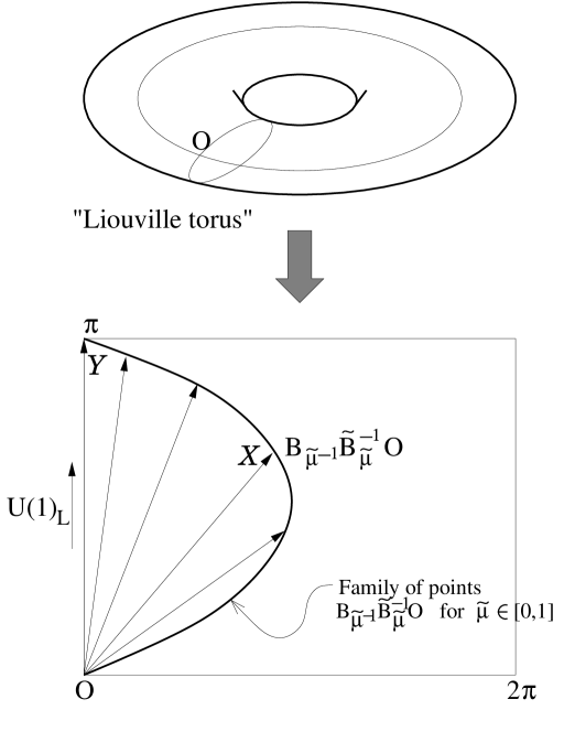
Figure 2: The relation between the hidden symmetry $U(1)_{L}$ and the Bäcklund transformations. We pick a point $O$ on a “Liouville torus” (for a finite-gap solution, this is an actual finite-dimensional torus). The solid curve $OXY$ represents the 1-parameter family of points $B_{\tilde{\mu}^{-1}}\tilde{B}_{\tilde{\mu}}^{-1}O$ parametrized by $\tilde{\mu}\in[0,1]$. When $\tilde{\mu}=1$ the interval $OY$ (where $Y=B_{1}\tilde{B}_{1}^{-1}O$) is the b-cycle of the torus. The symmetry $U(1)_{L}$ acts by shifts along this cycle. The arrow $OX$ represents the 1-parameter family of points $\exp\left[t\log(B_{\tilde{\mu}^{-1}}\tilde{B}_{\tilde{\mu}}^{-1})\right]O$ with $t\in[0,1]$. When $\tilde{\mu}\to 1$ the 1-parameter group $\exp\left[t\log(B_{1}\tilde{B}_{1}^{-1})\right]$ with $t\in[0,2]$ is $U(1)_{L}$.

One could imagine an ambiguity in the definition of $\xi_{\mu}$ and $\tilde{\xi}_{\tilde{\mu}}$, but we have the continuous families connecting $B_{\mu}$ to ${\bf 1}=B_{\infty}$ and $\tilde{B}_{\tilde{\mu}}$ to ${\bf 1}=\tilde{B}_{0}$. The existence of these continuous families allows us to define $\xi_{\mu}$ and $\tilde{\xi}_{\tilde{\mu}}$ unambiguously, see Fig. 1. The formula is:

$$\xi_{\mu}=-\sum_{p=0}^{\infty}{\mu^{-2p-1}\over 2p+1}{\partial\over\partial t_{2p+1}}$$ (40)

$$\tilde{\xi}_{\tilde{\mu}}=\sum_{p=0}^{\infty}{\tilde{\mu}^{2p+1}\over 2p+1}{\partial\over\partial\tilde{t}_{2p+1}}$$ (41)

These vector fields act on the rational solutions through the parameters $b_{j}$:

$$\xi_{\mu}.b_{j}={1\over 2}\log\left[{1-{\lambda_{j}/\mu}\over 1+{\lambda_{j}/\mu}}\right]b_{j}$$ (42)

$$\tilde{\xi}_{\tilde{\mu}}.b_{j}={1\over 2}\log\left[{1-{\tilde{\mu}/\lambda_{j}}\over 1+{\tilde{\mu}/\lambda_{j}}}\right]b_{j}$$ (43)

Let us consider the limit:

$$\xi=\lim\limits_{\epsilon\to 0+}(\xi_{e^{\epsilon}}-\tilde{\xi}_{e^{-\epsilon}})=\lim_{\epsilon\to 0+}\sum_{p=0}^{\infty}\left[-{e^{-(2p+1)\epsilon}\over 2p+1}{\partial\over\partial t_{2p+1}}-{e^{-(2p+1)\epsilon}\over 2p+1}{\partial\over\partial\tilde{t}_{2p+1}}\right]$$ (44)

We have:

$$\xi.b_{j}=-{\pi i\over 2}\;\mbox{sign}(\mbox{Im}(\lambda_{j}))\;b_{j}$$ (45)

We see that the trajectories of the vector field $\xi$ are periodic:

$$e^{2\xi}={\bf 1}$$ (46)

Therefore $\xi$ is the Hamiltonian vector field of an action variable. We denote $U(1)_{L}$ the corresponding hidden symmetry. Notice that $e^{\xi}$ exchanges $\tau_{+}$ and $\tau_{-}$ and therefore maps $\phi\mapsto-\phi$:

$$e^{\xi}=[\phi\mapsto-\phi]$$ (47)

The corresponding symmetry of the classical string is $\vec{n}\mapsto-\vec{n}$. We see that the discrete geometric ${\bf Z}_{2}$-symmetry (the “reflection” $\phi\mapsto-\phi$) is related to the continuous hidden symmetry $U(1)_{L}$ (generated by the higher Hamiltonians). This example is of the same nature as the relation between the anomalous dimension and the local charges discussed in [15].

In the language of free fermions, $B_{\mu}$ corresponds to the creation of the free fermion $\psi(\mu)$ from the left vacuum, and $\tilde{B}_{\tilde{\mu}}^{-1}$ to the creation of $\tilde{\psi}(\tilde{\mu})$ from the right vacuum. When $\mu\to\tilde{\mu}$, the leading term in the operator product expansion of $\psi(\mu)\tilde{\psi}(\tilde{\mu})$ is a $c$-number, and it cancels between $\tau_{+}$ and $\tau_{-}$ in (26). The shift of the charge of the left and right Dirac vacua leads to the exchange $\tau_{+}\leftrightarrow\tau_{-}$, and therefore Eq. (26) gives $\phi\mapsto-\phi$.

This construction essentially used the fact that $B_{1}\tilde{B}_{1}^{-1}=[\phi\mapsto-\phi]$. In fact for any real $\mu=\tilde{\mu}$ we have

$$B_{\mu}\tilde{B}^{-1}_{\tilde{\mu}}|_{\tilde{\mu}=\mu}=[\phi\mapsto-\phi]$$ (48)

This can be understood directly from (28), (30), (32), (33). First of all we have to explain the meaning of the left hand side of (48), because we defined $B_{\mu}$ only for large $\mu$ as a series in $1/\mu$ and $\tilde{B}_{\tilde{\mu}}$ for small $\tilde{\mu}$ as a series in $\tilde{\mu}$. Let us consider the null-surface limit (8) and construct $B_{\mu}$ and $\tilde{B}_{\tilde{\mu}}$ as a series in $\epsilon$, where $\epsilon$ is the small parameter of the null-surface perturbation theory defined in (8). In this perturbation theory we have $|\partial_{\sigma}\phi|<<|\partial_{\tau}\phi|$ and $|\phi|<<1$. The zeroth approximation to (28), (30) and (32), (33) is:

$$B_{\mu}\phi={1-\mu^{-2}\over 1+\mu^{-2}}\phi-{2\mu^{-1}\over 1+\mu^{-2}}\partial_{\tau}\phi$$ (49)

$$\tilde{B}_{\tilde{\mu}}\phi={1-\tilde{\mu}^{2}\over 1+\tilde{\mu}^{2}}\phi-{2\tilde{\mu}\over 1+\tilde{\mu}^{2}}\partial_{\tau}\phi$$ (50)

We see that in the leading order of the null-surface perturbation theory $B_{\mu}$ and $\tilde{B}_{\tilde{\mu}}$ both depend on $\mu$ and $\tilde{\mu}$ as rational functions. The higher orders are also rational functions of $\mu$ and $\tilde{\mu}$. Therefore in the null-surface perturbation theory $B_{\mu}$ and $\tilde{B}_{\tilde{\mu}}$ both have an unambiguous analytic continuation to finite values of $\mu$ and $\tilde{\mu}$. Therefore we can take $\mu=\tilde{\mu}$ and (48) follows from (28), (30), (32), (33) and (49), (50). This means that the generator of $U(1)_{L}$ which we defined in (44) as $\xi_{1}-\tilde{\xi}_{1}$ can be also defined as $\xi_{\mu}-\tilde{\xi_{\mu}}$ for any real $\mu$. For the rational solutions with all $\lambda_{j}$ having a nonzero imaginary part we have

$$(\xi_{\mu}-\tilde{\xi}_{\mu})-(\xi_{1}-\tilde{\xi}_{1})=0$$ (51)

for any $\mu\in{\bf R}$. Therefore $U(1)_{L}$ commutes with the Lorentz boosts which transform $\phi(t_{1},\tilde{t}_{1})$ to $\phi(\mu t_{1},\mu^{-1}\tilde{t}_{1})$.

4.2 Free field limit.

In the limit $\phi\to 0$ the equations of motion become

$$\partial_{t_{1}}\partial_{\tilde{t}_{1}}\phi=-4\phi$$ (52)

And the left and right Bäcklund transformations become:

$$B_{\mu}.\phi={1-{1\over 2\mu}{\partial\over\partial t_{1}}\over 1+{1\over 2\mu}{\partial\over\partial t_{1}}}\phi$$ (53)

$$\tilde{B}_{\tilde{\mu}}.\phi={1+{\tilde{\mu}\over 2}{\partial\over\partial\tilde{t}_{1}}\over 1-{\tilde{\mu}\over 2}{\partial\over\partial\tilde{t}_{1}}}\phi$$ (54)

This means that in the free field limit:

$${\partial\over\partial t_{2p+1}}\phi={1\over 2^{2p}}\left({\partial\over\partial t_{1}}\right)^{2p+1}\phi$$ (55)

$${\partial\over\partial\tilde{t}_{2p+1}}\phi={1\over 2^{2p}}\left({\partial\over\partial\tilde{t}_{1}}\right)^{2p+1}\phi$$ (56)

The generator of $U(1)_{L}$ acts as follows:

$$\xi.\phi=\lim_{\epsilon\to 0+}\log\left[{(2-e^{-\epsilon}\partial_{t_{1}})(2-e^{-\epsilon}\partial_{\tilde{t}_{1}})\over(2+e^{-\epsilon}\partial_{t_{1}})(2+e^{-\epsilon}\partial_{\tilde{t}_{1}})}\right]\phi=$$

$$=\lim_{\epsilon\to 0+}\log\left[{4\sinh\epsilon-\partial_{t_{1}}-\partial_{\tilde{t}_{1}}\over 4\sinh\epsilon+\partial_{t_{1}}+\partial_{\tilde{t}_{1}}}\right]\phi$$ (57)

The free field $\phi$ has an oscillator expansion:

$$\phi=\int{dk\over\sqrt{2\omega_{k}}}\left(\alpha_{k}e^{ik\sigma+i\omega_{k}\tau}+\overline{\alpha_{k}}e^{-ik\sigma-i\omega_{k}\tau}\right)$$ (58)

where $\omega_{k}=\sqrt{4+k^{2}}$. Eq. (57) implies that $U(1)_{L}$ is the oscillator number:

$$\xi.\alpha_{k}=\pi i\alpha_{k}$$

$$\xi.\overline{\alpha_{k}}=-\pi i\overline{\alpha_{k}}$$ (59)

This is in agreement with the results of [17] and shows that the $U(1)_{L}$ considered here is the same $U(1)_{L}$ as considered in [18, 17].

4.3 Action of $U(1)_{L}$ on a breather.

Consider $\lambda_{1}=\lambda=ie^{i\theta}|\lambda|$, $\lambda_{2}=\overline{\lambda}$, $b_{1}=be^{i\varphi}$ and $b_{2}=be^{-i\varphi}$ and denote $e^{\kappa}=b^{2}/\tan\theta$. We get

$$\tau_{\pm} = {2b^{2}\over\tan\theta}e^{-2t\sin\theta|\lambda|+2\tilde{t}\sin\theta|\lambda|^{-1}}\times$$

$$\left[\cosh(2t|\lambda|\sin\theta-2\tilde{t}|\lambda|^{-2}\sin\theta-\kappa)\pm\right.$$

$$\left.\pm i\tan\theta\cos(2t|\lambda|\cos\theta+2\tilde{t}|\lambda|^{-1}\cos\theta+2\varphi)\right]$$

Therefore

$$\tan{\phi\over 2}=\tan\theta{\cos(2t|\lambda|\cos\theta+2\tilde{t}|\lambda|^{-1}\cos\theta+2\varphi)\over\cosh(2t|\lambda|\sin\theta-2\tilde{t}|\lambda|^{-1}\sin\theta-\kappa)}$$ (62)

Remember that $t_{1}={1\over 4}(\tau+\sigma)$ and $\tilde{t}_{1}={1\over 4}(\tau-\sigma)$. The limit $\theta\to 0$ corresponds to a circular null-string. Indeed, with $|\lambda|=1$ Eqs. (6) and (62) imply in this limit that at $\tau=0$ we have $\int_{-\infty}^{\infty}d\sigma|\partial_{\sigma}\vec{n}|=2\pi$.

The generator of $U(1)_{L}$ acts on a breather by shifting the phase $\varphi$:

$$\xi={\pi\over 2}\mbox{sign}(\cos\theta){\partial\over\partial\varphi}$$ (63)

The general solution without kinks can be approximated by collections of breathers. The $U(1)_{L}$ will shift the phases of all the breathers by the same amount.

We have seen in Section 4.2 that the generator of $U(1)_{L}$ can be also understood as the nonlinear analogue of the oscillator number. On the other hand, we can see from Eqs. (62) and (63) that in the null surface limit

$$\xi\simeq{\pi\over 4}\left({\partial\over\partial t}+{\partial\over\partial\tilde{t}}\right)+\ldots$$ (64)

where dots denote the terms subleading in the null surface limit. The leading term is the energy of the string, and the subleading terms are the higher conserved charges. The fact that the energy is the oscillator number plus corrections was observed already in the work of H.J. de Vega, A.L. Larsen and N. Sanchez [37] .

4.4 The null-surface limit and the “improved” currents of [19, 20].

Eq. (62) shows that in the null-surface limit the parameters $\lambda_{j}$ are localized in the vicinity of $\pm i$:

$$\lambda_{j}=\pm i+O(\epsilon)$$ (65)

The action of the higher Hamiltonians on the parameters $b_{j}$ follows from (3.1):

$${\partial\over\partial t_{2p+1}}b_{j}=\lambda_{j}^{2p+1}b_{j}$$ (66)

Consider the following linear combination of the higher Hamiltonian vector fields:

$$\sum\limits_{p=0}^{l}{l!\over p!(l-p)!}{\partial\over\partial t_{2p+1}}b_{j}=\lambda_{j}(\lambda_{j}-i)^{l}(\lambda_{j}+i)^{l}b_{j}\simeq\epsilon^{l}b_{j}$$ (67)

We see that the vector fields

$$\Xi_{l}=\sum\limits_{p=0}^{l}{l!\over p!(l-p)!}{\partial\over\partial t_{2p+1}}$$ (68)

are generated by the “improved” currents; the vector field $\Xi_{l}$ is of the order $\epsilon^{l}$ in the null-surface perturbation theory.

The improved currents used in [19, 20] involve both left and right times. Let us introduce the improved Hamiltonian vector fields ${\cal G}_{k}$ which acts on the parameters $b_{j}$ in the following way:

$${\cal G}_{k}.b_{j}=\left(\lambda_{j}-{1\over\lambda_{j}}\right)\left[\left(\lambda_{j}+{1\over\lambda_{j}}\right)\right]^{2k}b_{j}$$ (69)

These vector fields are local and improved, in the sense that ${\cal G}_{k}\simeq\epsilon^{2k}$ in the null-surface limit (65). For example ${\cal G}_{0}={\partial\over\partial t_{1}}+{\partial\over\partial\tilde{t}_{1}}$, ${\cal G}_{1}={\partial\over\partial t_{3}}+{\partial\over\partial t_{1}}+{\partial\over\partial\tilde{t}_{1}}+{\partial\over\partial\tilde{t}_{3}}$ and ${\cal G}_{2}={\partial\over\partial t_{5}}+3{\partial\over\partial t_{3}}+2{\partial\over\partial t_{1}}+2{\partial\over\partial\tilde{t}_{1}}+3{\partial\over\partial\tilde{t}_{3}}+{\partial\over\partial\tilde{t}_{5}}$.

The Hamiltonian vector fields ${\partial\over\partial t_{2p+1}}+{\partial\over\partial\tilde{t}_{2p+1}}$ can be expressed through the improved vector fields:

$${\partial\over\partial t_{2p+1}}+{\partial\over\partial\tilde{t}_{2p+1}}=\sum\limits_{n=0}^{p}{2^{-2n}}U_{2p,2n}{\cal G}_{n}$$ (70)

where $U_{2p,2n}$ are the coefficients of the Chebyshev polynomials of the second kind:

$$U_{2p}(x)=\sum\limits_{k=0}^{p}U_{2p,2k}x^{2k}={(x+i\sqrt{1-x^{2}})^{2p+1}-(x-i\sqrt{1-x^{2}})^{2p+1}\over 2i\sqrt{1-x^{2}}}$$ (71)

In the null-surface perturbation theory ${\cal G}_{k}\simeq\epsilon^{2k}$. On the other hand, for $\lambda$ sufficiently close to $i$ or $-i$ we have

$${\pi i\over 2}\mbox{sign}(\mbox{Im}\;\lambda)={\pi\over 2}{\left(\lambda-\lambda^{-1}\right)\over\sqrt{4-\left(\lambda+\lambda^{-1}\right)^{2}}}=$$

$$={\pi\over 4}\sum\limits_{k=0}^{\infty}{(2k)!\over 2^{2k}(k!)^{2}}\left(\lambda-{1\over\lambda}\right)\left[{1\over 2}\left(\lambda+{1\over\lambda}\right)\right]^{2k}$$ (72)

This implies that

$$\xi=-{\pi\over 4}\sum\limits_{k=0}^{\infty}{(2k)!\over 2^{4k}(k!)^{2}}{\cal G}_{k}$$ (73)

We see that the generator of $U(1)_{L}$ is indeed an infinite sum of local conserved charges, with only finitely many terms participating at each order of the null-surface perturbation theory.

Eq. (73) can also be obtained from Eqs. (44) and (70) using the formula

$$\lim_{\epsilon\to 0+}\sum\limits_{p=0}^{\infty}{e^{-2p\epsilon}\over 2p+1}U_{2p}(x)={\pi\over 4}\left(1-x^{2}\right)^{-1/2}$$ (74)

5 Summary and discussion of $O(N)$ model.

In this section we will summarize our construction of the action variable for the sine-Gordon model and outline the analogous construction for the $O(N)$ sigma model.

5.1 The construction of the action variable for the sine-Gordon model.

The sine-Gordon model has infinitely many local conserved charges, which are in involution with each other. Therefore each solution $\phi(\tau,\sigma)$ defines an infinite-dimensional “invariant torus” which is defined as the orbit of $\phi(\tau,\sigma)$ under the Hamiltonian flows generated by the local conserved charges. This “invariant torus” consists of the solutions $\phi(\tau,\sigma,t_{3},\tilde{t}_{3},t_{5},\tilde{t}_{5},\ldots)$ where $t_{2n+1}$ and $\tilde{t}_{2n+1}$ are the “higher times” defined so that $\partial\over\partial t_{2n+1}$ and $\partial\over\partial\tilde{t}_{2n+1}$ are the Hamiltonian vector fields generated by the higher Hamiltonians. We denote $t_{1}={1\over 4}(\tau+\sigma)$ and $\tilde{t}_{1}={1\over 4}(\tau-\sigma)$.

The Bäcklund transformations $B_{\mu}$ and $\tilde{B}_{\tilde{\mu}}$ depend on the parameters $\mu$ and $\tilde{\mu}$. They can be understood as the shifts of the higher times; $B_{\mu}$ is the shift $t_{2n+1}\to t_{2n+1}-{\mu^{-2n-1}\over 2n+1}$ and $\tilde{B}_{\tilde{\mu}}$ is the shift $\tilde{t}_{2n+1}\to\tilde{t}_{2n+1}+{\tilde{\mu}^{2n+1}\over 2n+1}$. We have:

$$\begin{array}[]{l}{\partial\over\partial t_{1}}(B_{\mu}\phi+\phi)=-2\mu\sin(B_{\mu}\phi-\phi)\\ {\partial\over\partial\tilde{t}_{1}}(B_{\mu}\phi-\phi)={2\over\mu}\sin(B_{\mu}\phi+\phi)\end{array}$$ (75)

$$\begin{array}[]{l}{\partial\over\partial\tilde{t}_{1}}(\tilde{B}_{\tilde{\mu}}\phi+\phi)={2\over\tilde{\mu}}\sin(\tilde{B}_{\tilde{\mu}}\phi-\phi)\\ {\partial\over\partial t_{1}}(\tilde{B}_{\tilde{\mu}}\phi-\phi)=-2\tilde{\mu}\sin(\tilde{B}_{\tilde{\mu}}\phi+\phi)\end{array}$$ (76)

We define $B_{\mu}$ as a power series in $1/\mu$ and $\tilde{B}_{\tilde{\mu}}$ as a power series in $\tilde{\mu}$. Then we define the “logarithm” of the Bäcklund transformation. For each $\mu$ (large) and $\tilde{\mu}$ (small) the Hamiltonian vector field $\xi_{\mu,\tilde{\mu}}$ is generated by a linear combination of the local Hamiltonians, such that $e^{\xi_{\mu,\tilde{\mu}}}=B_{\mu}\tilde{B}^{-1}_{\tilde{\mu}}$. The explicit formula is $\xi_{\mu,\tilde{\mu}}=-\sum\left[{\mu^{-2p-1}\over 2p+1}{\partial\over\partial t_{2p+1}}+{\tilde{\mu}^{2p+1}\over 2p+1}{\partial\over\partial\tilde{t}_{2p+1}}\right]$. We defined $B_{\mu}$ perturbatively around $\mu=\infty$ and $\tilde{B}_{\tilde{\mu}}$ perturbatively around $\tilde{\mu}=0$. But we have seen that (at least on the rational solutions, which form a dense set) there is a well-defined limit $\xi=\lim\limits_{\mu\to 1,\tilde{\mu}\to 1}\xi_{\mu,\tilde{\mu}}$. Eqs. (75) and (76) suggest that $B_{1}\tilde{B}_{1}^{-1}$ is the transformation bringing $\phi$ to $-\phi$, and we have seen that this is indeed the case for rational solutions and in the null-surface perturbation theory. Therefore $e^{2\xi}$ is the identical transformation, which means that $\xi$ is generated by an action variable.

5.2 The $O(N)$ sigma-model.

The same arguments can be applied to the $O(N)$ sigma model. The Bäcklund transformations are defined by the same equations (3.1) and (3.1) as for $N=3$, but instead of a 3-dimensional vector $\vec{n}(\tau,\sigma)$ we have an $N$-dimensional vector $X$:

$$\begin{array}[]{l}\partial_{\tilde{t}_{1}}(B_{\mu}X-X)=-{1\over 2}(1+\mu^{-2})(B_{\mu}X,\partial_{\tilde{t}_{1}}X)(B_{\mu}X+X)\\[5.0pt] \partial_{t_{1}}(B_{\mu}X+X)={1\over 2}(1+\mu^{2})(B_{\mu}X,\partial_{t_{1}}X)(B_{\mu}X-X)\end{array}$$ (77)

$$\begin{array}[]{l}\partial_{t_{1}}(\tilde{B}_{\tilde{\mu}}X-X)=-{1\over 2}(1+\tilde{\mu}^{2})(\tilde{B}_{\tilde{\mu}}X,\partial_{t_{1}}X)(\tilde{B}_{\tilde{\mu}}X+X)\\[5.0pt] \partial_{\tilde{t}_{1}}(\tilde{B}_{\tilde{\mu}}X+X)={1\over 2}(1+\tilde{\mu}^{-2})(\tilde{B}_{\tilde{\mu}}X,\partial_{\tilde{t}_{1}}X)(\tilde{B}_{\tilde{\mu}}X-X)\end{array}$$ (78)

We conjecture that the Bäcklund transformations correspond to the shift of times if we define them perturbatively as series in $1/\mu$ and $\tilde{\mu}$. (We do not know a proof of this fact for the $O(N)$ model.) But we can also define the Bäcklund transformations perturbatively using the null-surface perturbation theory. In the null-surface perturbation theory the small parameter is $1/|p|=1/|\partial_{\tau}X|$ and $\partial_{\sigma}X$ remains finite. In the limit $|p|\to\infty$ we observe that (77) and (78) are solved by:

$$B_{\mu}X={1-\mu^{-2}\over 1+\mu^{-2}}X-{2\mu^{-1}\over 1+\mu^{-2}}{\partial_{\tau}X\over|\partial_{\tau}X|}$$ (79)

$$\tilde{B}_{\tilde{\mu}}X={1-\tilde{\mu}^{2}\over 1+\tilde{\mu}^{2}}X+{2\tilde{\mu}\over 1+\tilde{\mu}^{2}}{\partial_{\tau}X\over|\partial_{\tau}X|}$$ (80)

The corrections to (79), (80) by the higher powers of $1/|\partial_{\tau}X|$ involve higher derivatives in $\tau$ and $\sigma$ and depend on $\mu$ as rational functions. When $\mu$ is large we can expand these corrections in powers of $\mu^{-1}$. Therefore the definition of the Bäcklund transformation $B_{\mu}$ as a power series in $1/|\partial_{\tau}X|$ agrees with the usual definition as a power series in $\mu^{-1}$, but does not require $\mu$ to be large.

As we did for the sine-Gordon model, we can define $\xi_{\mu}$ as the Hamiltonian vector field $\log B_{\mu}$ and $\tilde{\xi}_{\tilde{\mu}}=\log B_{\tilde{\mu}}$. Now we want to put $\mu=\tilde{\mu}$. There is a potential problem here, because $B_{\mu}$ was defined as a series in $1/\mu$ and $\tilde{B}_{\tilde{\mu}}$ as a series in $\tilde{\mu}$. But as we discussed, we can also define $B_{\mu}$ and $\tilde{B}_{\tilde{\mu}}$ in the null-surface perturbation theory using $1/|\partial_{\tau}X|$ as a small parameter. Then there is no problem doing the analytical continuation to $\mu=\tilde{\mu}$, because at every order of the $1/|\partial_{\tau}X|$ perturbation theory $B_{\mu}$ is a rational function of $\mu$. (For example, the zeroth order is given by (79).) Equations (77), (78), (79) and (80) imply that for $\mu=\tilde{\mu}$ we have $B_{\mu}\tilde{B}^{-1}_{\mu}X=-X$. Therefore

$$e^{\xi_{\mu}-\tilde{\xi}_{\mu}}=[X\mapsto-X]$$

This implies that the Hamiltonian vector field $\xi_{\mu}-\tilde{\xi}_{\mu}$ is generated by an action variable. This vector field is independent of the choice of $\mu$ (in the perturbation theory in $1/|\partial_{\tau}X|$) because of the uniqueness of the action variable. For the explicit calculation it would be convenient to choose $\mu=1$, because with this choice it is manifest that the action variable is a combination of the local charges which is left-right symmetric. The vector field ${\partial\over\partial{\mu}}(\xi_{\mu}-\tilde{\xi}_{\mu})$ is zero in the perturbation theory because of the relations between the left and right charges discussed in Section 3 of [17].

Note in the revised version: see [38] for the discussion of the $O(N)$ model.

References

• [1] S. Frolov, A.A. Tseytlin, ”Semiclassical quantization of rotating superstring in $AdS_{5}\times S^{5}$”, JHEP 0206 (2002) 007, hep-th/0204226.
• [2] A.A. Tseytlin, ”Semiclassical quantization of superstrings: $AdS_{5}\times S^{5}$ and beyond”, Int. J. Mod. Phys. A18 (2003) 981, hep-th/0209116.
• [3] J.G. Russo, ”Anomalous dimensions in gauge theories from rotating strings in $AdS_{5}\times S^{5}$,” JHEP 0206 (2002) 038, hep-th/0205244.
• [4] J. A. Minahan, K. Zarembo, “The Bethe-Ansatz for N=4 Super Yang-Mills,” JHEP 0303 (2003) 013, hep-th/0212208.
• [5] S. Frolov, A.A. Tseytlin, “Multi-spin string solutions in $AdS_{5}$ x $S^{5}$,” Nucl.Phys. B668 (2003) 77-110, hep-th/0304255.
• [6] S. Frolov, A. A. Tseytlin, “Quantizing three-spin string solution in $AdS_{5}\times S^{5}$,” JHEP 0307 016 (2003), hep-th/0306130.
• [7] M. Kruczenski, “Spin chains and string theory”, hep-th/0311203.
• [8] M. Kruczenski, A.V. Ryzhov, A.A. Tseytlin, “Large spin limit of $AdS_{5}$ x $S^{5}$ string theory and low energy expansion of ferromagnetic spin chains”, Nucl.Phys. B692 (2004) 3-49, hep-th/0403120.
• [9] G. Mandal, N.V. Suryanarayana, S.R. Wadia, “Aspects of Semiclassical Strings in AdS5”, Phys.Lett. B543 (2002) 81, hep-th/0206103.
• [10] I. Bena, J. Polchinski, R. Roiban, “Hidden Symmetries of the $AdS_{5}\times S^{5}$ Superstring”, Phys.Rev. D69 (2004) 046002, hep-th/0305116.
• [11] M. Wolf, “On Hidden Symmetries of a Super Gauge Theory and Twistor String Theory”, hep-th/0412163.
• [12] L. Dolan, C.R. Nappi, E. Witten, “A Relation Between Approaches to Integrability in Superconformal Yang-Mills Theory”, JHEP 0310 (2003) 017, hep-th/0308089.
• [13] L. Dolan, C.R. Nappi, E. Witten, “ Yangian Symmetry in D=4 Superconformal Yang-Mills Theory”, hep-th/0401243.
• [14] L. Dolan, C.R. Nappi, “Spin Models and Superconformal Yang-Mills Theory”, hep-th/0411020.
• [15] A. Mikhailov, “Anomalous dimension and local charges”, hep-th/0411178.
• [16] K. Pohlmeyer, “Integrable Hamiltonian Systems and Interactions through Quadratic Constraints”, Comm. Math. Phys. 46 (1976) 207-221.
• [17] A. Mikhailov, “Plane wave limit of local conserved charges”, hep-th/0502097.
• [18] A. Mikhailov, “Notes on fast moving strings”, hep-th/0409040.
• [19] G. Arutyunov, M. Staudacher, “Matching Higher Conserved Charges for Strings and Spins”, JHEP 0403 (2004) 004, hep-th/0310182
• [20] J. Engquist, “Higher Conserved Charges and Integrability for Spinning Strings in $AdS_{5}$ x $S^{5}$”, JHEP 0404 (2004) 002, hep-th/0402092.
• [21] M. Kruczenski, A. Tseytlin, “Semiclassical relativistic strings in $S^{5}$ and long coherent operators in N=4 SYM theory”, hep-th/0406189.
• [22] H.J. De Vega, A. Nicolaidis, “Strings in strong gravitational fields”, Phys. Lett. B295 214-218; H. J. de Vega, I. Giannakis, A. Nicolaidis, “String Quantization in Curved Spacetimes: Null String Approach”, Mod.Phys.Lett. A10 (1995) 2479-2484, hep-th/9412081.
• [23] A. Mikhailov, “Speeding Strings”, JHEP 0312 (2003) 058, hep-th/0311019.
• [24] G. Arutyunov, S. Frolov, “Integrable Hamiltonian for Classical Strings on $AdS_{5}\times S^{5}$”, JHEP 0502 (2005) 059, hep-th/0411089.
• [25] N. Beisert, V. A. Kazakov, K. Sakai, K. Zarembo, “The Algebraic Curve of Classical Superstrings on $AdS_{5}\times S^{5}$”, hep-th/0502226.
• [26] L. F. Alday, G. Arutyunov, A. A. Tseytlin, “On Integrability of Classical SuperStrings in $AdS_{5}\times S^{5}$”, hep-th/0502240.
• [27] J. Minahan, “Higher Loops Beyond the SU(2) Sector”, JHEP 0410 (2004) 053, hep-th/0405243; “The SU(2) sector in AdS/CFT”, hep-th/0503143.
• [28] N. Beisert, V. A. Kazakov, K. Sakai, “Algebraic Curve for the SO(6) sector of AdS/CFT”, hep-th/0410253.
• [29] V.A.Kazakov, A.Marshakov, J.A.Minahan, K.Zarembo, “Classical/quantum integrability in AdS/CFT”, JHEP 0405 (2004) 024, hep-th/0402207.
• [30] V.A. Kazakov, K. Zarembo, “Classical/quantum integrability in non-compact sector of AdS/CFT”, hep-th/0410105.
• [31] S. Schafer-Nameki, “The Algebraic Curve of 1-loop Planar N=4 SYM”, hep-th/0412254.
• [32] A. Mikhailov, “A nonlocal Poisson bracket of the sine-Gordon model”, hep-th/0511069.
• [33] O. Babelon, D. Bernard, “Affine Solitons: A Relation Between Tau Functions, Dressing and Bäcklund Transformations”, hep-th/9206002.
• [34] L.D. Faddeev, L.A. Takhtajan, “Hamiltonian Methods in the Theory of Solitons”, Springer-Verlag, Berlin, 1987.
• [35] S. Kharchev, A. Marshakov, A. Mironov, A. Morozov, A. Zabrodin, “Towards unified theory of $2d$ gravity”, Nucl. Phys. B380 (1992) 181-240, hep-th/9201013.
• [36] A. Neveu, N. Papanicolaou, “Integrability of the classical scalar and symmetric scalar - pseudoscalar contact Fermi interactions in two-dimensions”, Commun.Math.Phys.58:31,1978.
• [37] H.J. de Vega, A.L. Larsen, N. Sanchez, “Semi-Classical Quantization of Circular Strings in De Sitter and Anti De Sitter Spacetimes”, Phys.Rev. D51 (1995) 6917-6928, hep-th/9410219.
• [38] A. Mikhailov, “Bäcklund transformations, energy shift and the plane wave limit”, hep-th/0507261.