Causal structures and holography
We explore the description of bulk causal structure in a dual field theory. We observe that in the spacetime dual to a spacelike non-commutative field theory, the causal structure in the boundary directions is modified asymptotically. We propose that this modification is described in the dual theory by a modification of the micro-causal light cone. Previous studies of this micro-causal light cone for spacelike non-commutativite field theories agree with the expectations from the bulk spacetime. We describe the spacetime dual to field theories with lightlike non-commutativity, and show that they generically have a drastic modification of the light cone in the bulk: the spacetime is non-distinguishing. This means that the spacetime while being devoid of closed timelike or null curves, has causal curves that are “almost closed”. We go on to show that the micro-causal light cone in the field theory agrees with this prediction from the bulk.
1. Introduction
The advent of the AdS/CFT correspondence [1] has revolutionised our understanding of quantum gravity, and has led to important insights into both gravity and strongly coupled gauge dynamics. However, a considerable number of important conceptual questions remain open, especially those pertaining to a detailed understanding of gravitational dynamics. In particular, we still lack full understanding of how field theory on a fixed background can be approximated by a local theory with dynamical metric in the bulk.
One major issue is that the bulk spacetime has some dynamically determined causal structure, whereas the dual field theory lives in flat space, with the usual fixed light cone. The description of the bulk causal structure from the dual point of view has been the subject of a number of investigations in the AdS/CFT correspondence. Bulk causality in global AdS spacetime is consistent with boundary causality [2]; for example, propagation through the bulk is never faster than propagation along the boundary (this was extended to asymptotically AdS spacetimes satisfying the weak energy condition in [3]). When we restrict to Poincaré-invariant states, the light cone in the boundary directions will automatically agree in the bulk and boundary, and the focus is on understanding the causal structure in the bulk radial direction. In [4], Kabat and Lifschytz proposed a scale/radius description, where causality in the radial direction is enforced by a speed limit on varying scale size in the field theory. If we violate Poincaré invariance, for example by considering a black hole spacetime in the bulk (corresponding to finite temperature in the field theory), the bulk causal structure will not in general agree with the field theory one even in the boundary directions. The extension of Kabat & Lifschytz’s analysis to such cases was considered in [5]. However, for asymptotically AdS spacetimes, the causal structure changes only in the interior of the spacetime, which makes it difficult to pose sharp questions about the interpretation of these changes in the field theory.
In this paper, we will consider extreme examples of changes in the bulk causal structure: spacetimes dual to non-commutative field theories. Since the non-commutativity changes the structure of the field theory even in the ultraviolet, the bulk spacetime is no longer asymptotically AdS. The point of interest to us is that the causal structure of the bulk spacetime is drastically modified: in the limit as we approach the boundary, the light cone in the boundary directions ceases to depend on the directions in which non-commutativity is turned on. Thus, propagation through the bulk can take us outside the flat space light cone in these directions. We want to understand how this is described from the field theory point of view. One would expect that the non-locality of the non-commutative field theory plays a crucial role, and we will argue that this is indeed the case. In [6, 7, 8], it was argued that the non-locality leads to modifications of the micro-causal light cone: in particular, it does not agree with the naive causal structure of the background flat space the field theory is defined in. We will show in a simple toy example, scalar non-commutative field theory, that these modifications agree with the light cone in the boundary directions of the bulk spacetime. Extending this result to non-commutative gauge theories is somewhat tricky owing to issues related to absence of local gauge invariant observables. Nevertheless, we will argue based on the known properties of correlation functions of gauge invariant operators, that we indeed expect to see a modified causal structure in the field theory.
We study the modifications of the causal structure for both the spacelike non-commutativity, previously studied in [7, 8], and for lightlike non-commutativity. The lightlike case is especially interesting because the corresponding spacetime geometry has a very radical modification of its causal structure. The spacetime becomes non-distinguishing, meaning that distinct points of the spacetime have the same causal future and past. Such a spacetime ‘almost has’ closed timelike curves (CTCs); it is in the borderline area between being clearly causally well-behaved and clearly pathological. Since the discovery of supersymmetric spacetimes with CTCs [9], there has been a lot of discussion of whether spacetimes with CTCs are admissible backgrounds in string theory. Most of the discussion has centered on some string version of chronology protection; for example [10] related chronology violation in AdS/CFT to unitarity loss, while [11] argue for a holographic chronology protection mechanism. In light of the latter proposal that holography could ‘cut off’ the region of CTCs, it is remarkable to observe that lightlike non-commutativity provides an example where a non-distinguishing spacetime has a well-behaved holographic dual description. We will suggest that the non-distinguishing character of this spacetime is reflected in the micro-causal structure of the lightlike non-commutative field theory. Understanding this case may also be helpful for understanding the dual description of plane wave spacetimes, as they are also on the borderline (although they are distinguishing, they are not globally hyperbolic, and do not have Cauchy surfaces). Non-distinguishing examples of pp-waves have also recently been constructed [12, 13, 14].
In the next section, we will review the construction of the dual spacetime for a spacelike non-commutative deformation of SYM [15, 16], and discuss the features of the bulk light cone. In Section Causal structures and holography, we consider the micro-causality in spacelike non-commutative field theory. We review the argument of [7, 8] that the micro-causality condition for spacelike non-commutative field theories is to be imposed inside a ‘light wedge’. In [7, 17] it was argued that for a non-commutative field theory on with , the breaking of Lorentz symmetry by non-commutativity would enlarge the region where the commutator of fields is non-vanishing from the usual light cone to a light wedge respecting the unbroken symmetry. As discussed in [8], the non-local character of the field theory plays an essential role in this enlargement. We show that this light wedge agrees with the bulk results and suggest a framework for exploring these issues in non-commutative gauge theories.
We then turn to the consideration of lightlike non-commutativity. In Section Causal structures and holography we construct the bulk spacetime by applying the “Null Melvin Twist”, a solution-generating technique discussed in [18, 19]. We get our solution by applying this twist to the extremal D3-brane, and then taking a decoupling limit. We demonstrate that the spacetime is non-distinguishing using the arguments of [12, 13], and briefly sketched in the appendix. We then show in Section Causal structures and holography that this spacetime is the holographic dual description of a theory with lightlike non-commutativity. (This solution and its dual description were previously obtained in [20].) It was shown in [21] that theories with lightlike non-commutativity are well-defined quantum field theories, albeit with non-local interactions. We thus have an example where a non-distinguishing spacetime has a non-perturbative quantum description. We go on to show that any spacetime dual to a generic theory with lightlike non-commutativity will be non-distinguishing. Extending our arguments from the spacelike case, we are able to demonstrate that the micro-causal structure in a simple scalar field theory with lightlike non-commutativity reproduces the predicted causal structure inferred from these non-distinguishing spacetimes. Commutators of local operators can be shown to vanish only at equal light cone time, respecting the unbroken Galilean subgroup of the Lorentz group (in the presence of lightlike non-commutativity). We further argue that subtleties relating to gauge invariance will not change the result significantly in the case of lightlike non-commutative gauge theories and conclude with a brief discussion. Some details of the field theory calculations and more general solutions obtained by the null Melvin twist are described in the appendices. A short summary of the essential physical ideas can be found in [22].
2. Spacelike non-commutativity: bulk light cone
We begin by discussing the situation in the case of spacelike non-commutative field theories. In this section, we explore the causal properties of the dual spacetime, and note that it has a deformed light cone even in the asymptotic region. We consider geodesics which remain at large radius to study the features of this light cone.
The string frame metric for the spacetime dual to spacelike non-commutative SYM is [15, 16]
| (2.1) |
There are non-trivial 3-form and 5-form fluxes in the above background and a varying dilaton, but these are not going to be relevant to our present discussion. as usual denotes the AdS radius and is related to the non-commutative parameter in the field theory as .
This dual geometry is obtained by thinking of the spacelike non-commutative Yang-Mills theory as arising as the low-energy limit of the theory on D3-branes in a constant background B-field. The supergravity configuration sourced by these D3-branes can be obtained by introducing the B-field through a twisting operation. To twist, start from the D3-branes in empty space, T-dualize to D2-branes, and then consider instead the compactification of the D2-brane solution on a tilted torus. T-dualizing along this tilted direction will give D3-branes in a B-field background. Applying this twisting operation to the D3-brane metric, and then taking the decoupling limit to focus on the near-horizon geometry, gives the spacetime (2.1).
While the geometry (2.1) is close to for small , it has vastly different asymptotics. In particular, as for , which will give rise to the deformation of the light cone we are interested in. This makes it hard to define a boundary for the spacetime, but we will show later that the deformation of the light cone is nonetheless reflected in field theory micro-causality behaviour.
Suppose we look at the metric induced on a fixed surface with , i.e., we think of the bulk defining an UV regulated version of the non-commutative field theory. In this case, the induced metric on the surface (ignoring the part) reads:
| (2.2) |
At any fixed value of , we can rescale the coordinates to convert (2.2) into a flat metric on . However, the scaling is non-homogeneous, and in particular, as we remove the cutoff we will have to scale the shrinking directions by a diverging amount, whereas we would expect the field theory background to be defined by a homogeneous rescaling of coordinates, as in the usual commutative case. This would lead us to conclude that the relevant light cone for the field theory is independent of the non-commuting directions . Alternately, as is apparent from the full metric (2.1), the metric factor in front of the non-commuting directions falls off faster than that in front of the part, and therefore should not contribute to the light cone asymptotically.
We would like to argue that this change in the bulk light cone is reflected in observable quantities in the dual field theory. One approach would be to study the two-point function in the boundary, which should be determined, by the usual logic, by the bulk-to-bulk propagator for the appropriate supergravity field in the background (2.1) in the limit . By examining the behaviour of the bulk Greens functions we should be able to extract the detailed properties of the bulk light cone, and in particular its asymptotic behaviour. However, the Klein-Gordon equation is rather formidable (it is related to the Mathieu equation [16]), and so explicit determination of the propagator is difficult. Nevertheless, we can approximate it by studying the geodesics in the bulk spacetime. We will now show that the bulk light cone indeed degenerates into a light wedge asymptotically in the geodesic approximation.
Ignoring motion on the part of the geometry and setting for simplicity, we have the equation for timelike geodesics
| (2.3) |
where , with the affine parameter along the geodesics. The Killing symmetries and determine the conserved energy and momenta , respectively. The geodesic motion reduces to a classical problem for the zero energy trajectories of a particle in an effective potential :
|
|
(2.4) |
Let us consider geodesics that travel an infinitesimal distance in the radial direction. Choose with such that . Then we have
| (2.5) |
This allows us to approximately integrate the geodesic equations to obtain, for instance,
| (2.6) |
and
| (2.7) |
One can clearly make the distance travelled by the geodesics in individual directions large, by choosing appropriate values for the momenta. However, the motion is confined to the region in the immediate vicinity of the classical bulk light cone, as the proper interval remains small:
|
|
(2.8) |
where we made use of the fact that .
Thus, bulk geodesics can relate points inside the light cone given by
| (2.9) |
and as we remove the cutoff by taking , the light cone in the boundary directions will approach a ‘light wedge’:
| (2.10) |
This is the advertised modification of the bulk causal structure. Although we have restricted our attention to bulk geodesics, we will have essentially obtained the same answer by looking at say the free scalar propagator for (2.1). Having obtained a prediction from the bulk perspective, we now turn to looking for signs of this change in the causal structure in the field theory.
3. Micro-causality in non-commutative field theories
The field theory dual to the geometry (2.1) is SYM theory in flat four-dimensional spacetime, with a constant non-commutativity parameter . We want to show that the above ‘light wedge’ structure is also naturally reflected in this field theory. As we are dealing with a Lorentz non-invariant non-local field theory, it is not a priori obvious what the causal relations in the field theory are. We will see that if we define the light cone of the field theory to be the micro-causal light cone, that is, the boundary of the region where the commutator of elementary fields is non-vanishing, then it will agree with the light wedge predicted from the bulk.
3.1. Non-commutative scalar field dynamics: a toy model
The micro-causal light cone for spacelike non-commutative field theories was studied in [7], and further clarified recently in [8]. In [7], a heuristic argument was given for a modification of the micro-causality condition. The non-commutativity in a spatial , , breaks Lorentz invariance in the field theory from . As a result it was suggested that one should not demand causal behaviour with respect to the full invariance, but rather only with respect to the smaller symmetry . This corresponds to the invariance of the light wedge obtained above (although the reduced symmetry is not sufficient to fix the form of the light cone).
That is, the authors of [7] propose that instead of requiring that the fields (labeled collectively as ) commute (or anti-commute for fermions) across spacelike separated points,
| (3.1) |
the appropriate micro-causality condition for non-commutative field theories would be to only impose
| (3.2) |
where is the separation in the commuting directions,
| (3.3) |
For example with we have .
This argument has two weaknesses: since it appeals to the violation of Lorentz invariance, it would appear to apply whenever we have Lorentz violating interactions, and not only in non-commutative field theories. Also, the symmetry does not really determine a light cone; while the light wedge used in (3.2) respects , so does the original light cone of (3.1). In [8], these weaknesses were addressed by performing an explicit perturbative calculation of the commutator for non-commutative field theory, showing that the micro-causality condition (3.2) is correct for spacelike non-commutative field theories, whereas (3.1) remains correct for theories with local Lorentz violating interactions. This shows that the non-local character of the non-commutative interactions is important.
We will give a brief derivation of this result [8]. The authors consider spacelike non-commutative theory in for simplicity,
| (3.4) |
The strategy is to calculate the expectation value of the Heisenberg picture field operator between two states and , obtained by time-evolution of the perturbative vacuum ,
| (3.5) |
Given a perturbation expansion of
| (3.6) |
one can study to determine the domains where it is guaranteed to vanish. We have used translational invariance to write . This will provide us with the definition of the micro-causal light cone in field theory.
The calculation of proceeds in the standard fashion and some of the details can be found in Appendix Acknowledgements. The main point is that we can write in an integral representation as
| (3.7) |
where the integrand generically takes the form
| (3.8) |
The integration variables are the independent light cone momenta after imposition of momentum conservation and are constants. The details of the interaction are contained in the kernel . In writing (3.7), we have rewritten various amplitudes in terms of light cone variables for ease of computation: .
The behaviour of the integrand in the complex space parameterised by is crucial in determining the convergence properties of the integral. For instance, at tree-level in perturbation theory we have
| (3.9) |
Given this, the usual contour deformation arguments can be used to show that
| (3.10) |
which is the expected result for the free field theory (recall that the non-commutative deformation affects quadratic terms only by the presence of irrelevant phase factors). To be precise, assuming without loss of generality, for we can rotate the contour of integration for the integral as in integrating (and for ). The two integrals then are convergent and moreover the finite answers cancel in the difference; hence the commutator vanishes. For timelike separation , there is no deformation of the contour that gives a convergent integral; hence generically the difference of the two integrals is non-vanishing and we are led to (3.10).
For non-commutative field theories, we intuitively expect to see the first sign of interesting effects at one-loop, i.e., in , for we have qualitatively new feature in perturbation theory in the form of non-planar Feynman graphs. We should expect that the phase factors involved in the non-commutative interaction modify the properties of and thereby deform the nature of the light cone. Detailed calculations [8] show that this expectation is indeed borne out. We in fact find that (see Appendix Acknowledgements for details)
| (3.11) |
implying that
| (3.12) |
with is as defined in (3.3). This follows by repeating the argument for the convergence of the integrals with the modified integrand (3.11). So we see that the micro-causality condition in spacelike non-commutative field theories is modified at one-loop. In particular, note that the presence of the non-commutative interactions demand that the expectation value of the field commutator vanish only outside a light-wedge as surmised earlier333As an interesting aside, it should be possible to show the modification of the micro-causality condition using the 1PI effective action derived for non-commutative theory in [23]. The inverse propagator (in momentum space) for this theory is , with . This propagator has extra poles in the complex momentum plane at , where is the restriction of the momentum to the commutative sub-space. The presence of these poles induces a delta function for the momentum along the non-commutative directions. This ultra localization in momentum space is the origin of the light-wedge (3.3)..
This micro-causal light wedge agrees with the prediction of the spacetime in the previous section. This agreement should be considered as qualitative evidence that the micro-causal structure in the field theory is indeed related to the light cone determined by the bulk spacetime.
3.2. Micro-causality in non-commutative gauge theories
We have shown that the micro-causality in a scalar non-commutative field theory agrees with the bulk light cone. However, this scalar field theory is only a toy model, and there are important differences which make it unclear if this behaviour will generalize to the non-commutative gauge theory which is actually dual to the bulk spacetime (2.1). We will now review the salient differences, and argue that we nevertheless still expect to see a reflection of the bulk light cone in the micro-causality of the non-commutative gauge theory.
The first difference has to do with the structure of UV divergences in gauge theories. As remarked in the footnote above, the modification of the micro-causality condition is related to the IR divergences seen in perturbation theory for non-commutative dynamics. Although explicit calculation confirms the presence of such IR poles in a general non-commutative gauge theory [24], they will be absent for the non-commutative SYM theory we’re interested in because of the supersymmetry. Thus, the modification of the micro-causality condition for gauge theories can’t arise in the same way as it did in the scalar theory studied above.
There is however another important difference, which we will argue can lead to a similar modification of the micro-causality condition by a more subtle route. In non-commutative gauge theories there are no gauge invariant local operators (essentially because translation in the non-commutative directions is equivalent to a gauge transformation), so it is unclear why we should even consider the micro-causal structure based on local fields. An over-complete set of non-local gauge invariant observables was constructed in [25, 26, 27]. The idea was to string a local operator such as (which is of course gauge invariant in the commutative limit) with an open Wilson line and take its Fourier transform. This defines a local gauge invariant operator in momentum space . They calculated correlation functions of the operators and showed that the correlation functions grow exponentially in momenta
| (3.13) |
This exponential growth of correlation functions may also be seen from the supergravity dual [26]. In writing the above we have dropped some regularization dependent terms which will be unimportant for properly renormalised correlators. We want to suggest that the exponential growth of the correlation functions signals a modification of the micro-causality conditions for these operators.
The clue comes from studies of a similar behaviour in another non-local quantum field theory discovered in the past decade, little string theory, which is a Poincaré invariant theory in six dimensions with a mass scale , living on the world-volume of NS5-branes. These theories admit gauge invariant local operators in momentum space and their correlation functions also grow exponentially in momenta [28]. This fact was used in [29] to argue that little string theories are quasi-local theories, and that a modified notion of micro-causality could be defined for such theories.
In local quantum field theories, correlation functions in position space, the Wightman functions, are to be smeared with suitable test functions to generate observables. We would therefore normally define a micro-causality condition by smearing the Wightman function with test functions of spacelike separated support. However, to do so, the Wightman functions need to be tempered distributions, so that we can use the usual Schwartz space of test functions. Physically this amounts to the correlation functions in momentum space growing at most polynomially.
In the non-local theory, where momentum space correlators grow exponentially, the Wightman functions are rather singular distributions and the allowed space of test functions is restricted. In this case test functions are required to be real analytic in position space, which precludes local observables (cf.[29] for references and rigorous arguments). This prevents us from defining a micro-causality condition in the usual way, as we cannot smear with test functions of spacelike separated support.
In [29], it was proposed that we can still study micro-causality in these cases, by considering the analytic structure of the Wightman functions at points where they make sense as functions. Usually micro-causality implies permutation symmetry of Wightman functions: for example, for spacelike separated points and . However, for the more singular Wightman functions in a non-local theory, the region of analytic behaviour is restricted. In the case of little string theories, [29] observed that the Wightman function is analytic only for , and proposed that the micro-causality condition be replaced by requiring permutation symmetry of Wightman functions in this restricted region. The usual commutativity condition is modified by the presence of poles in the region .
While a detailed analysis of the analyticity properties of the non-commutative gauge theory Wightman functions is beyond the scope of the current paper, we believe that it should be possible to construct an analogous argument to determine the micro-causality properties associated with the gauge-invariant operators , relating the restriction to the light-wedge (3.12) seen from the spacetime point of view to the fact that the momentum space correlator (3.13) is growing only along the non-commutative directions. Recent discussions of microcausality conditions in non-commutative theories can be found in [30, 31, 32].
It is also useful to note that agreement is expected: the micro-causality conditions for an interacting theory on the boundary ought to be captured by a free-field theory in the bulk in the large limit (where the supergravity approximation is expected to valid), because the correct micro-causality conditions in the field theory stem from the quantum 1PI propagator. This might seem a bit puzzling in the context of the previous discussion of non-commutative scalar field theories, as we see (in appendix A) that the effect of non-commutativity arose from non-planar diagrams in the field theory. However, these non-planar contributions are associated with the non-commutative interactions, and are not suppressed by large power counting; in their absence, the spacetime dual for non-commutative SYM would have been just , rather than the spacetime (2.1) with its complicated asymptotics.
4. Generating spacetimes by null Melvin twist
We next want to extend the discussion to the spacetimes dual to lightlike non-commutative field theories. We will begin by presenting the derivation of these solutions, using a particular solution generating technique in supergravity, called the null Melvin twist [18, 19]. This is slightly more complicated than the twist used to obtain the geometry in the spacelike case, and will add a B-field oriented along a lightlike direction. While some of the solutions we are interested in have been obtained previously in the literature [20], re-deriving them in this way will simplify the discussion of generalisations. A nice summary of the solution generating scheme we use and some classifications of solutions can be found in [33]. 4.1. The null Melvin twist
The solution generating scheme is:
1. Start with a solution of IIA/IIB supergravity, with a non-compact translationally invariant direction; the corresponding Killing vector will be taken to be .
2. Boost the geometry in the direction by an amount . Note that this is just a coordinate change, which effectively adds momentum charge to the solution we start with.
3. Now perform a T-duality along , to get to a solution of IIB/IIA supergravity.
The above steps will typically add a fundamental string charge to the solution we start with. However, if the Killing field can be paired with a timelike Killing field (so that our starting solution has isometry), then no charge is added. Instead Step 2 is trivial as the geometry is boost invariant. Step 3 is then just a diagonal T-duality.
4. The Twist: Assume that we have in addition to the Killing field , some other rotational or translational isometries. We would like to perform a non-diagonal T-duality by combining these isometries with that generated by . Schematically, denoting the one-forms dual to the additional isometries by , we perform a twist (a coordinate transformation) by replacing
| (4.1) |
Here parameterises the amount of twisting.
5. We now T-dualize the geometry back to IIA/IIB along . The twist followed by the T-duality is effectively a non-diagonal T-duality.
6. Boost the solution by along . The purpose of this boost is in part to undo the original boost performed.
7. Now, we perform a double scaling limit, wherein the boost is scaled to infinity and the twist to zero keeping
| (4.2) |
The null Melvin twist transformations in steps 4 through 7 can be thought of as converting the string solution into a fluxbrane, followed by a boost and scaling to end up with a null isometry.
4.2. Null Melvin twist of the D3-brane solution
Let us apply this transformation to the D3-brane geometry. The extremal D3-brane geometry is a solution of Type IIB supergravity with metric:
| (4.3) |
with
| (4.4) |
The metric (4.3) is supported by a five-form flux. Since the flux turns out to be insensitive to the null Melvin twist we will not write it explicitly.
The geometry (4.3) has a Lorentz symmetry along the world-volume directions , and so we will not have any charge added during the first two steps. The twisted T-duality implemented in steps 4 and 5 requires us to pick a direction to do the twisting. The simplest choice turns out to be the translationally invariant directions and . Performing the twist as
| (4.5) |
we obtain the following geometry:
|
|
(4.6) |
Apart from the NS-NS 3-form flux written above the metric is in addition supported by a five-form flux (which is the same as for the original D3-brane solution (4.3)). The sequence of operations 1 to 7 maps a constant dilaton solution back to a constant dilaton solution for this particular case. Note that the solution (4.6) is asymptotically flat.
In deriving (4.6) we have used the translational isometries to perform the twisted T-duality. We could just as well have used some angular isometries, such as the rotation isometry in the plane, or isometries of the . In such cases, we would generate asymptotically plane wave, rather than asymptotically flat, spacetime; however, since this asymptotic region will be lost once we take the decoupling limit, the interesting causal features of the plane wave (such as 1-dimensional boundary or non-global hyperbolicity) would not enter our story. These cases are briefly discussed in Appendix Acknowledgements, although the essential physical point of interest is exemplified adequately by (4.6).
4.3. Near-horizon geometry of null Melvin twisted D3-brane
Our main interest is to identify interesting generalisations of the AdS/CFT correspondence, so we now consider an appropriate decoupling limit of the geometry (4.6), to obtain a new duality relating the low energy degrees of freedom on the twisted D3-brane to a supergravity geometry. For the D3-brane geometry (4.3), we know that the near horizon limit corresponding to decoupling the closed string modes from the open string modes on the D3-brane is obtained by dropping the in the harmonic function given in (4.4)[34]. For the solution (4.6), we want to ensure that the effect of the twist survives in the decoupling limit. Thus the appropriate limit is analogous to the Seiberg-Witten scaling for non-commutative field theories [35]. This again amounts to dropping the from the harmonic function (4.4), now in the new metric (4.6). The resulting geometry is given by
|
|
(4.7) |
where we have introduced light cone coordinates and . In addition to the NS-NS B-flux there is also a five-form flux, which is identical to that supporting the solution. The metric only differs from the metric written in Poincaré coordinates by the term proportional to . This solution was previously derived in [20]. They considered the solution to Type IIB supergravity that was known to be dual to SYM deformed by spacelike non-commutativity [15, 16], and boosted it to derive (4.7). As in the case of spacelike non-commutativity, it is difficult to define a conformal boundary for this spacetime. The correspondence to the field theory is derived by thinking of the field theory as living on the D3-branes that source the full geometry (4.6), and taking the low-energy limit.
We now show that this solution is non-singular, and non-distinguishing. We show that it is non-singular by observing that all the curvature invariants for (4.7) are the same as for , and that the spacetime is geodesically complete. The additional contributions to the curvature from the term proportional to will involve , so they will not change the curvature invariants. Geodesic completeness can be shown either by observing that the metric is conformal to a pp-wave,
|
|
(4.8) |
(where we have set and in the second line used ), and appealing to the results of [36], or by explicitly studying the geodesics. We will discuss timelike geodesics in the geometry (4.8) in Section Causal structures and holography. The essential point is that the motion in the radial direction is confined to a finite range and inertial observers are unable to escape towards the asymptotic region (cf., (6.3), where it is clear that geodesics cannot access the region , or equivalently , due to a potential barrier). Thus, though we have diverging curvatures in the large region, the spacetime is non-singular.
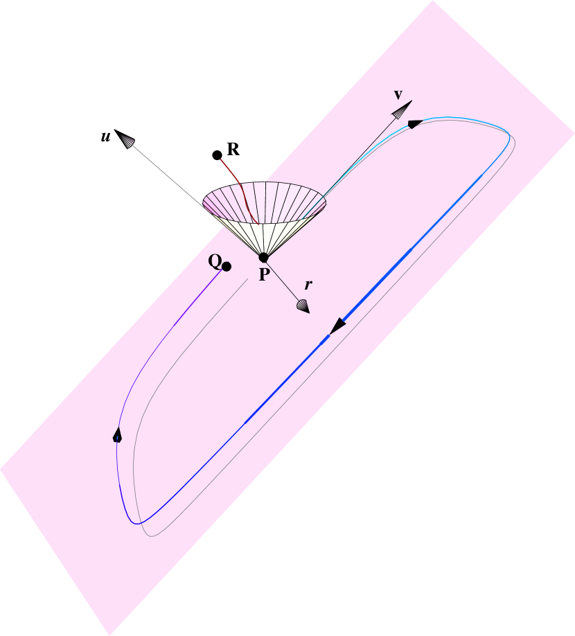
To show that the spacetime is non-distinguishing, it is easiest to use the representation (4.8) of the metric as conformal to a pp-wave, and use the results of [12, 13]. Since causal properties are invariant under conformal transformations, the causal character of our spacetime is determined by that of the pp-wave spacetime within the parenthesis in (4.8). In [12, 13] it was shown that these pp-wave spacetimes are non-distinguishing. Causal curves that connect a point in the spacetime to any point , with and arbitrary values of were explicitly constructed. This shows that the causal future of is the entire region , as depicted in Fig 1. In the terminology of [12], the metric (4.8) written in the coordinate is conformal to a super-quadratic pp-wave, as grows faster than a quadratic for large . We give an explicit construction of the causal curve from to (in the coordinates) in Appendix Acknowledgements.
5. The holographic dual field theory
As can be seen either from the lightlike nature of the B-field in the spacetime geometry (4.6) or from the alternative derivation444 In [20], the solution was obtained by starting from the holographic dual to NCYM with spacelike non-commutativity and then boosting. of this geometry in [20], the dual field theory description of the geometry (4.8) is a , non-commutative Super Yang-Mills (NCYM) on with a constant lightlike non-commutativity parameter for .
5.1. Well behavedness of observables in the field theory
Such lightlike non-commutativity was first discussed in [21], where it was shown that theories with lightlike non-commutativity behave like field theories with non-local interactions. This is in contradistinction with the case of timelike non-commutativity, where we have a string theoretic behaviour due to the non-decoupling of excited open string oscillators. The crucial difference between the two cases is the following [21]: in the case of timelike non-commutativity, we start from a D-brane background and turn on electric fields on the brane world-volume [37]. There is however a critical limit to the electric field (T-dual to there being a maximum velocity – speed of light), and at the critical point the open strings become effectively tensionless. The timelike theory is defined by zooming in on this critical region, and as a result one ends up with a finite effective string tension. In the case of lightlike non-commutativity, we turn on both electric and magnetic fields, and it is easy to see that this combination doesn’t lead to a critical electric field. Alternatively, one can think of the lightlike theory as a boosted version of the spacelike theory, where there is clearly no critical behaviour. Thus, this dual is a well behaved field theory with non-local interactions. Hence it is quite surprising that the dual geometry (4.8) exhibits some causal pathology.
To understand better the physics of lightlike non-commutative field theories we can consider observables in these theories, such as the correlation function of local operators . These can be calculated at strong ’t Hooft coupling using the using the usual bulk-boundary correspondence. It transpires that massless minimally coupled scalar fields in the bulk geometry (4.8) satisfy a Mathieu equation which is very similar to that obtained in [16] for the geometry (2.1). Of course the parameters appearing in the equation have a different dependence on momenta, as should be expected given the different symmetries of the geometries. This implies that the correlation functions are schematically similar to the spacelike case. Likewise, one can consider gauge invariant observables built with open Wilson lines as discussed in [26] and check that these are also well behaved and in fact will be exponential in the momenta. In summary, there is no reason from a field theory perspective that lightlike non-commutative field theories should be pathological, which makes the bizarre causal structure of the dual spacetime geometry all the more interesting.
5.2. Genericity of non-distinguishingness for lightlike non-commutative field theories
We have shown above that the supergravity background dual to lightlike non-commutative SYM is a non-distinguishing spacetime. We will now show that any well defined field theory will produce a non-distinguishing holographic dual when we deform it by adding some lightlike non-commutativity.
Consider any field theory defined in the usual Wilsonian sense, by its ultraviolet modes. From the UV/IR correspondence for gauge/gravity duality [38], we know that the field theory ultra-violet corresponds to the infra-red region of the supergravity dual. For field theories on one can without loss of generality assume that the holographic dual geometry is of the following warped product form:
| (5.1) |
where is an effective radial coordinate on the transverse space with metric . If the field theory approaches a conformal fixed point in the UV, the large behaviour will be asymptotically for some compact Einstein manifold . Our argument will however be general enough to include more exotic field theories which do not arise from nice conformal fixed points in the UV, such as the Klebanov-Strassler cascade [39].
We would like to turn on lightlike non-commutativity in the field theory. We have seen above that this is achieved by a Null Melvin Twist on the dual geometry (5.1). The Poincaré invariance of the field theories on implies that there are no fluxes that prevent us from carrying through the steps involved in the duality chain. A null Melvin twist of (5.1) will lead to the following geometry:
| (5.2) |
The question is then what the effect of the additional term is on the causal structure; this depends on the particular form of . For field theories with a conformally invariant fixed point in the UV, the large behaviour of is , giving the same kind of asymptotics as in the particular case we studied, and hence implying that for such cases, the metric (5.2) is non-distinguishing. The same is true for the appropriate to the Klebanov-Strassler geometry [39], so non-commutative deformations of this theory also have non-distinguishing duals, see Appendix Acknowledgements for the explicit metric.
Thus, we see that the UV behaviour of the field theory is responsible for the dual supergravity background being causally ill-behaved. It follows that infrared modifications of the field theory will not remove the causal pathologies, as they do not change the asymptotics of the dual spacetimes. For example, the thermal version of the non-commutative theory will be dual to a spacetime with a black hole in it, but this will still be non-distinguishing. For completeness, we present the metric for the thermal version of the lightlike non-commutative SYM in Appendix Acknowledgements.
6. Causality in lightlike non-commutative theories
We now attempt to understand the origin of the non-distinguishing character of the spacetime (4.8) from the field theory perspective. As with the case of spacelike non-commutativity, it will be instructive to first understand the behaviour of the bulk light cone in the asymptotic region. We will then proceed to look at the micro-causality condition in field theory and show that the perturbative micro-causal light cone is modified so as to be consistent with the characteristics of the bulk spacetime. As in section 3, we consider a simple scalar field theory as a model, but it seems reasonable to expect that this micro-causal structure will be independent of the details of the particular field theory we consider.
6.1. Lightlike non-commutativity: bulk light cone
Our derivation of the bulk light cone for the lightlike non-commutative field theories will proceed in a fashion analogous to the spacelike case discussed in Section Causal structures and holography. We will focus once again on the properties of the bulk light cone in the asymptotic region of the spacetime, which for (4.8) will be the region or .
Let us consider the induced metric on a surface of fixed , so as to discern the causal properties in the cut-off lightlike non-commutative field theory. This induced metric is (in what follows we will ignore the directions)
| (6.1) |
which of course is the metric on flat once we rescale the coordinates appropriately. However, if we restrict to homogeneous rescaling of the coordinates, the metric (6.1) degenerates to a one dimensional metric due to the dominance of for large . We then expect the bulk light cone to degenerate to a Galilean causal structure, in which any two points are causally related unless .
The above argument for the asymptotic bulk light cone can be made precise by considering the two-point function. For the metric (4.8), the free scalar wave equation is still the Mathieu equation, making explicit determination of the propagator tricky. We will therefore concentrate again on a geodesic approximation to the propagator. Let us begin by considering timelike geodesics in the geometry (4.8),
| (6.2) |
where , with the affine parameter along the geodesics. The Killing symmetries , and determine conserved energies and momenta , respectively. The geodesic motion reduces to a classical problem for the zero energy trajectories of a particle in an effective potential555From the form of it is clear that geodesics never reach for , thereby preventing inertial observers from being subject to large tidal forces resulting from the diverging curvatures in that region. This is the hitherto alluded to characteristic that demonstrates geodesic completeness of (4.8). :
|
|
(6.3) |
Let us consider geodesics that travel an infinitesimal distance in the radial () direction. Choose with such that . Then we have
| (6.4) |
This allows us to approximately integrate the geodesic equations to obtain,
| (6.5) |
It is obvious from (6.5) that one can make the distance travelled by the geodesics in individual directions large by choosing appropriate momenta. However, the motion is confined to the region in the immediate vicinity of the classical bulk light cone, as
| (6.6) |
Thus, bulk geodesics can relate points inside the effective light cone given by
| (6.7) |
which limits as to the Galilean invariant light wedge. Causal properties are then determined by just the value of coordinate. We see that the point is in the past of if irrespective of the other coordinates.
6.2. Micro-causality in lightlike non-commutative field theories
Let us now study the micro-causal light cone for this case of lightlike non-commutativity, following the discussion of the spacelike case given earlier. First of all, we can use the simpler argument of [7] to suggest the appropriate micro-causality condition for this case. Suppose we have a field theory in with , where we use lightcone coordinates for . This non-commutative deformation will break the Lorentz group down to a Galilean group. The natural Galilean invariant micro-causal relation to consider is
| (6.8) |
We can use the argument of [8] as briefly reviewed in Section Causal structures and holography to show that the lightlike non-commutative field theory in fact has such a micro-causality condition, while a local quantum field theory with Galilean invariance will still have the usual commutation relations (3.1).
For sake of simplicity we consider the non-commutative theory introduced in (3.4); we will calculate the perturbative behaviour of the field commutator expectation value to probe the micro-causality condition. In fact, the calculation proceeds in a manner similar to the spacelike non-commutative case, but for a few essential differences in the details of the kernels. As in that case there is no difference from commutative theory at the tree level i.e., for . Once again interesting effects show up at the one-loop contribution to the commutator, thanks to the contribution from the non-planar diagrams. The calculation is outlined in Appendix Acknowledgements. We find that the non-planar graphs give us one-loop contribution
| (6.9) |
In writing the above we have retained only the dominant contribution at large momentum (for this is the part that determines the convergence properties) and is a vector with components . We have furthermore
| (6.10) |
and as usual, is the same as in the commutative field theory.
In order to ascertain the micro-causality condition, we need to figure out the domain where is guaranteed to vanish. This can be done by looking at the analytic properties of . Assuming without loss of generality , we see that will be convergent only for . However, for we encounter a divergence from the term proportional to in the exponential. Hence we are forced to conclude that there is no domain in the complex plane where the integral of is absolutely convergent. This in particular implies that we are generically going to encounter a non-vanishing value of . The only special case is when when we expect will indeed vanish. This is not apparent from (6.9) and (6.10), since these are written in a light cone quantization scheme. Intuitively, one expects this to arise simply from the fact that this is indeed the ‘equal time’ commutation relation for light cone quantization. To summarise, the micro-causality condition for this lightlike non-commutative field theory is indeed as given by (6.8).
As we have emphasized in the spacelike non-commutative case, it would be challenging to extend this computation to the non-commutative Yang-Mills theory which is actually dual to the bulk spacetime. Once again, the appropriate framework for exploring these ideas would be to look at the details of the analytic behaviour of the Wightman functions. However, as argued in the spacelike case, the micro-causal light cone for the field theory ought to be in agreement with the causal properties of the supergravity dual. So, it is again encouraging to find that the results in the scalar field theory exhibit qualitative agreement with the bulk spacetime. Since the bulk behaviour was intimately associated with the non-distinguishing character of this spacetime, we might even say that this non-distinguishing character is not only consistent in string theory, but in fact necessary to reproduce this behaviour in the dual field theory.
7. Discussion
We have studied modifications of the causal structure of the bulk spacetime in the AdS/CFT correspondence, by considering the changes in the geometry dual to a non-commutative deformation of the field theory. We pointed out that these deformations cause radical changes in the bulk causal structure. For spacelike non-commutativity, the light cone in the boundary directions asymptotically becomes independent of the non-commutative directions. For lightlike non-commutativity, the modification is even stronger, producing a non-distinguishing spacetime, in which points are always connected by a causal curve unless they have the same value of ‘light-cone time’.
We compared the asymptotic bulk light cone to the micro-causal light cone in a scalar non-commutative field theory, following [7, 8]. In this toy example we were able to show that the micro-causal light cone was in complete agreement with the bulk predictions. As we have already remarked, we think it reasonable to expect this agreement to extend to non-commutative gauge theory, and have suggested a possible way to infer this rigorously.
The essential issue in considering non-commutative gauge dynamics is the absence of local gauge invariant observables in position space. However, any bulk calculation of correlation function in strongly coupled non-commutative gauge theory will exhibit the deformed light cone structure. From the point of AdS/CFT correspondence it is imperative that this structure be reproduced from the field theory side as well. In fact, as discussed in [26, 40] there is an excellent agreement between the result for the correlation function of gauge invariant open Wilson loop operators in the field theory (obtained by summing up ladder diagrams) and the bulk prediction. Furthermore, given the nature of observables in the non-commutative gauge theory, this agreement is expected to be universal. Since the bulk two point function is sensitive to the deformation of the light cone, it seems quite natural to expect the same in the field theory.
These results provide a new connection between the causal structure in the bulk and in the boundary. However, the full encoding of the bulk causal structure in the dual field theory description remains an important open problem. In particular, we have not addressed the very interesting question of how the bulk causal structure is encoded when the Poincaré invariance in broken only in the interior (as in black hole solutions).
The discovery that a non-distinguishing spacetime is related via the AdS/CFT duality to a well-defined quantum field theory is of interest in its own right. It suggests that such geometries may be more respectable as string theory backgrounds than one might have expected. The usual objection to non-distinguishing backgrounds, that a small deformation can convert them into a solution with closed timelike curves, is here circumvented by the fact that the non-distinguishing character is a consequence of the behaviour of the light-cone in the asymptotic region, where corrections are suppressed. That is, although there are almost closed timelike curves, they do not remain within a compact region of the spacetime. These solutions deserve further investigation.
Acknowledgements
We would like to thank Henriette Elvang, Sean Hartnoll, Gary Horowitz and especially Chong-Sun Chu for illuminating discussions. VH and MR are supported by the funds from the Berkeley Center for Theoretical Physics, DOE grant DE-AC03-76SF00098 and the NSF grant PHY-0098840. SFR is supported by the EPSRC Advanced Fellowship.
Appendix A: Derivation of light-wedge
We present in this appendix a short derivation of the micro-causality condition in non-commutative field theories. Further details can be found in [8].
As discussed in Section Causal structures and holography, we are interested in calculating the matrix element of the field commutator in perturbation theory. The field theory we consider will be non-commutative theory in with Lagrangian (3.4). In what follows bold face letters will denote spatial vectors etc., in . We will also have use for light cone coordinates and the vectors transverse to the light cone directions will be denoted as .
Working within the framework of canonical quantization, one can write the interaction picture field as
| (A.1) |
where .
As usual it is possible to pass between the interaction and Heisenberg pictures:
| (A.2) |
We will make use of this to evaluate the matrix element (3.5) and consider the states and obtained by evolving the perturbative vacuum by the evolutions operator .
For the theory the quantities of interest are the tree-level term and the one-loop term . The former is just the usual free field propagator; the presence of non-commutative interactions play no interesting role for the quadratic terms in the Lagrangian (3.4). In fact, we have
| (A.3) |
which may be written in the form (3.7), using the identity
| (A.4) |
In writing the above we have passed over to light cone representation of momenta for convenience. Hence we obtain
| (A.5) |
Completing the Gaussian integrals over in (A.5) we find the integral representation of with the kernel as given in (3.9).
From this representation of one can ascertain the domains where the commutator is required to vanish. As discussed in Section Causal structures and holography the strategy is to ascertain the possible contour rotations for the integral. Depending on the convergence of the integrals of , the two terms contributing to mutually cancel. This is where we see the origin of the micro-causality condition in the field theory. The contour rotations that lead to cancellation of the two integrals work only for spacelike separated points and not for points which are in causal contact.
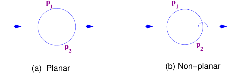
The calculation of proceeds in a similar fashion. We get contributions for the non-commutative theory from two kinds of one-loop diagrams: planar and non-planar. The planar diagrams are very similar to those of the commutative theory and do not change the micro-causal structure. The non-planar diagrams introduce extra momentum dependent phase factors through the term. These phase factors play an important role in modifying the properties of . The relevant Feynman diagrams are shown in Fig 2.
We will concentrate exclusively on the non-planar contribution to the commutator. The phase factor originating from the interaction for the non-planar graph is
| (A.6) |
Ignoring numerical coefficients we can write
| (A.7) |
where
| (A.8) |
is of the general form described in (3.8), and the kernel is
| (A.9) |
is a function of the momenta that grows like a polynomial and hence doesn’t play any role in our discussions. Readers interested in its precise form can consult [8]. In deriving the above we have made use of the identity (A.4) given above to convert the momentum integrals over to integrals over and over the light cone component labeled here as respectively. Note that while we have lumped a lot of the details of the interaction in the factor , we are keeping the phase factor explicitly, since it is an exponential function of the momenta.
We now analyze the large momentum behaviour of (A.9) by completing the squares and performing the resulting integral (setting ). So far our discussion has been independent of the precise nature of the non-commutative interaction. We will see that there is a distinction between the spacelike non-commutative and lightlike non-commutative cases. The essential point is that the large momentum behaviour of (A.9) depends on the nature of the non-commutative interaction, and so we will treat these two cases separately.
A.1. Spacelike non-commmutativity
For spacelike non-commutative theories we will choose only along the spatial directions transverse to our light cone coordinates, thus having . So we can write (A.9) as
|
|
(A.10) |
One interesting aspect is that the large momentum behaviour of is independent of the non-commutative parameter . Using the expressions for we find at the end of the day,
| (A.11) |
In contrast to the tree-level result, we see that the convergence properties at one-loop (for non-planar contributions) depend only on the light cone defined with respect to the commuting directions in spacetime. Once again going through the possible contour rotations leads us to conclude that the commutator is required in this case to vanish outside the light-wedge as in (3.12).
A.2. Lightlike non-commutativity
Here we choose the non zero components of to be those with , with denoting the spatial directions in . This in particular implies that the phase factor will be
| (A.12) |
Hence calculating the kernel reduces to
|
|
(A.13) |
The integrals over are easily done, but unlike the case of spacelike non-commutativity discussed previously we find that the dominant term for large depends explicitly on . In fact, we have
| (A.14) |
In writing the above we have retained only the dominant contribution at large momentum (for it is the part that determines the convergence properties). If we consider the contour rotations for the integrals, continuing leaves us with a divergent integral (assuming without loss of generality ) for . One might wonder about continuing into the lower half-plane i.e., ; this doesn’t help because the integral then diverges at small . Hence there is no contour rotation that will allow us to obtain a finite answer, so we are led to conclude that the correct micro-causality condition is as given in (6.8).
Appendix B: Non-distinguishing property the spacetime
In this appendix, we demonstrate directly that the spacetime (4.8),
| (B.1) |
is non-distinguishing. In particular, we exhibit a causal curve connecting a point in the spacetime to any point , with arbitrarily small, and arbitrary values of , where and capture the 2 transverse directions and the 5 angular directions of the , respectively.
Since along any future directed causal curve the coordinate must increase, we can parameterise our curve by , so that
| (B.2) |
Then the causality condition implies that for all ,
| (B.3) |
where we define . For simplicity, we break up the curve into five components; the first and last being null curves in the plane, while the middle three move in the , , and directions, respectively. Letting each component take equal interval, these curves, with , join the points
|
|
(B.4) |
with the quantities and as defined below. Choosing this joining to be linear, we can write the component curves explicitly as
|
|
(B.5) |
with
|
|
(B.6) |
where we define the constants
|
|
(B.7) |
These ensure that the curve is connected, joining the points (B.4), and (B.6) ensure that and are null. Finally, to guarantee causality of and , we must choose bounded from below by
| (B.8) |
Physically, we want to take advantage of the large- region, where the term in the metric (B.1) allows causality for large changes in the other coordinates. A schematic representation of such a causal curve in space is sketched in Fig 1. Note that this is only possible for nonzero .
Hence, a crucial feature of our construction of the causal curve is that it involves arbitrarily large radii, scaling as inverse positive power of . In other words, it is exactly due to the asymptotic region that the spacetime is non-distinguishing. As commented above, this bears two important consequences: it lets us extract this causal property directly from the dual boundary theory, and it pacifies possible causality-violating quantum fluctuations.
Likewise, in the tamer case of the spacetime (2.1), the holographic dual to the SYM with spacelike non-commutativity, it is important that the light wedge structure appears only asymptotically. For otherwise, if the spacetime exhibited a light-wedge structure even in the interior, then any two points separated only in the non-commutative directions (along the wedge) would have identical past/future sets—the spacetime would be non-distinguishing. But we know that this is not the case, as (2.1) admits a time function: it is stably causal and therefore distinguishing.
Appendix C: Other solutions generated by null Melvin twist
In this appendix we write down metrics generated by applying the null Melvin twist transformations on other geometries.
C.1. Twisting along angular isometries
Instead of performing the null Melvin twist on the planar directions we could instead have used some angular directions. The most general such configuration can be generated by starting with the D3-brane solution written as (4.3), with
|
|
(C.1) |
We can in this case perform the null Melvin twist by
| (C.2) |
This leads to the metric
|
|
(C.3) |
While the metric (C.3) is interesting in its own right, we will mostly focus on the simpler case presented in (4.6).
C.2. Non-extremal null Melvin twisted D3-brane geometry
To obtain the supergravity dual to thermal lightlike non-commutative SYM, we need to start with a non-extremal D3-brane geometry and carry out the null Melvin twist duality transformation. Recall that the metric for the non-extremal D3-brane takes the form
| (C.4) |
with
| (C.5) |
In this case the non-extremality of the solution implies that we no longer have the symmetry along the D3-brane world-volume. However, is still a good spacelike Killing vector and we have the requisite symmetries to proceed with the duality chain.
Carrying out Steps 1 through 7 outlined in Section 2.1, we obtain the metric for the null Melvin twisted non-extremal D3-brane:
|
|
(C.6) |
Here as in (4.6), we have twisted along the non-compact directions for simplicity. We have also refrained from writing down the explicit expressions for the p-form fields supporting the solution. This solution was also discussed in [41].
The metric is a bit more complicated than (4.6), but it is easy to check that in the decoupling limit (replacing ) the asymptotic form of the metric coincides with that of (4.8). Since it is the asymptotic region that is responsible for the non-distinguishing character of the spacetime, we conclude that (C.6) is also a non-distinguishing spacetime. That is, since the decoupling limit of (C.6) and (4.8) have a similar large behaviour, two points which are sufficiently far away from the black hole ought to have the same causal future/past, implying that the spacetime is non-distinguishing.
C.3. Null Melvin twist of Klebanov-Strassler
The Klebanov-Strassler solution is given by the metric
| (C.7) |
where denotes the metric of the deformed conifold and is a radial coordinate that measures the size of the base. The solution for the warp factor is given as an integral expression
| (C.8) |
and the metric is supported by both five-form and three-form fluxes. Asymptotically, this metric approaches the Klebanov-Tseytlin (KT) geometry [42] with
| (C.9) |
where is the length scale set by the number of fractional branes and the IR scale where we should revert to the original solution (C.8).
For our purposes it will suffice to note that we have a flat metric on which is non-trivially warped. Thus we can carry out the null Melvin twist along the translational isometries. Carrying out the steps in the duality chain we will end up with a metric that is analogous to (4.8). Apart from the fact that we have to replace the by the base of the deformed conifold we have no new change. In the large limit, where we have the KT solution, the base is the Einstein space . The astute reader will have realized that we have already taken the near horizon limit in writing the metric (C.7). So the spacetime dual to lightlike non-commutative deformed cascade theory is
| (C.10) |
which asymptotically looks like
| (C.11) |
The only difference from the non-distinguishing spacetime (4.8) is the logarithmic pieces. However, it is easy to check that these do not affect the causal structure of the spacetime in an essential manner.
References
- [1] O. Aharony, S. S. Gubser, J. M. Maldacena, H. Ooguri, and Y. Oz, “Large N field theories, string theory and gravity,” Phys. Rept. 323 (2000) 183–386, hep-th/9905111.
- [2] G. T. Horowitz and N. Itzhaki, “Black holes, shock waves, and causality in the AdS/CFT correspondence,” JHEP 02 (1999) 010, hep-th/9901012.
- [3] S. Gao and R. M. Wald, “Theorems on gravitational time delay and related issues,” Class. Quant. Grav. 17 (2000) 4999–5008, gr-qc/0007021.
- [4] D. Kabat and G. Lifschytz, “Gauge theory origins of supergravity causal structure,” JHEP 05 (1999) 005, hep-th/9902073.
- [5] J. P. Gregory and S. F. Ross, “Looking for event horizons using UV/IR relations,” Phys. Rev. D 63 (2001) 104023, hep-th/0012135.
- [6] M. Chaichian, K. Nishijima and A. Tureanu, “Spin-statistics and CPT theorems in noncommutative field theory,” Phys. Lett. B568, 146 (2003) hep-th/0209008.
- [7] L. Alvarez-Gaume and M. A. Vazquez-Mozo, “General properties of noncommutative field theories,” Nucl. Phys. B668 (2003) 293–321, hep-th/0305093.
- [8] C.-S. Chu, K. Furuta, and T. Inami, “Locality, causality and noncommutative geometry,” hep-th/0502012.
- [9] J. P. Gauntlett, J. B. Gutowski, C. M. Hull, S. Pakis, and H. S. Reall, “All supersymmetric solutions of minimal supergravity in five dimensions,” Class. Quant. Grav. 20 (2003) 4587–4634, hep-th/0209114.
- [10] G. W. Gibbons and C. A. R. Herdeiro, “Supersymmetric rotating black holes and causality violation,” Class. Quant. Grav. 16 (1999) 3619–3652, hep-th/9906098.
- [11] E. K. Boyda, S. Ganguli, P. Horava, and U. Varadarajan, “Holographic protection of chronology in universes of the Goedel type,” Phys. Rev. D67 (2003) 106003, hep-th/0212087.
- [12] J. L. Flores and M. Sanchez, “Causality and conjugate points in general plane waves,” Class. Quant. Grav. 20 (2003) 2275–2292, gr-qc/0211086.
- [13] V. E. Hubeny, M. Rangamani, and S. F. Ross, “Causal inheritance in plane wave quotients,” Phys. Rev. D69 (2004) 024007, hep-th/0307257.
- [14] J. L. Flores and M. Sanchez, “On the geometry of pp-wave type spacetimes,” gr-qc/0410006.
- [15] A. Hashimoto and N. Itzhaki, “Non-commutative Yang-Mills and the AdS/CFT correspondence,” Phys. Lett. B465 (1999) 142–147, hep-th/9907166.
- [16] J. M. Maldacena and J. G. Russo, “Large N limit of non-commutative gauge theories,” JHEP 09 (1999) 025, hep-th/9908134.
- [17] M. Chaichian and A. Tureanu, “Jost-Lehmann-Dyson representation and Froissart-Martin bound in quantum field theory on noncommutative space-time,” hep-th/0403032.
- [18] M. Alishahiha and O. J. Ganor, “Twisted backgrounds, pp-waves and nonlocal field theories,” JHEP 03 (2003) 006, hep-th/0301080.
- [19] E. G. Gimon, A. Hashimoto, V. E. Hubeny, O. Lunin, and M. Rangamani, “Black strings in asymptotically plane wave geometries,” JHEP 08 (2003) 035, hep-th/0306131.
- [20] M. Alishahiha, Y. Oz, and J. G. Russo, “Supergravity and light-like non-commutativity,” JHEP 09 (2000) 002, hep-th/0007215.
- [21] O. Aharony, J. Gomis, and T. Mehen, “On theories with light-like noncommutativity,” JHEP 09 (2000) 023, hep-th/0006236.
- [22] V. E. Hubeny, M. Rangamani, and S. F. Ross, “Causally pathological spacetimes are physically relevant,” gr-qc/0504013.
- [23] S. Minwalla, M. Van Raamsdonk, and N. Seiberg, “Noncommutative perturbative dynamics,” JHEP 02 (2000) 020, hep-th/9912072.
- [24] A. Matusis, L. Susskind, and N. Toumbas, “The IR/UV connection in the non-commutative gauge theories,” JHEP 12 (2000) 002, hep-th/0002075.
- [25] N. Ishibashi, S. Iso, H. Kawai, and Y. Kitazawa, “Wilson loops in noncommutative Yang-Mills,” Nucl. Phys. B573 (2000) 573–593, hep-th/9910004.
- [26] D. J. Gross, A. Hashimoto, and N. Itzhaki, “Observables of non-commutative gauge theories,” Adv. Theor. Math. Phys. 4 (2000) 893–928, hep-th/0008075.
- [27] S. R. Das and S.-J. Rey, “Open Wilson lines in noncommutative gauge theory and tomography of holographic dual supergravity,” Nucl. Phys. B590 (2000) 453–470, hep-th/0008042.
- [28] S. Minwalla and N. Seiberg, “Comments on the IIA NS5-brane,” JHEP 06 (1999) 007, hep-th/9904142.
- [29] A. Kapustin, “On the universality class of little string theories,” Phys. Rev. D63 (2001) 086005, hep-th/9912044.
- [30] M. Chaichian, M. N. Mnatsakanova, K. Nishijima, A. Tureanu and Y. S. Vernov, “Towards an axiomatic formulation of noncommutative quantum field theory,” arXiv:hep-th/0402212.
- [31] D. H. T. Franco and C. M. M. Polito, “A new derivation of the CPT and spin-statistics theorems in non-commutative field theories,” hep-th/0403028.
- [32] D. H. T. Franco, “On the Borchers class of a non-commutative field,” J. Phys. A 38, 5799 (2005) hep-th/0404029.
- [33] A. Hashimoto and K. Thomas, “Dualities, twists, and gauge theories with non-constant non-commutativity,” JHEP 0501, 033 (2005) hep-th/0410123.
- [34] J. M. Maldacena, “The large N limit of superconformal field theories and supergravity,” Adv. Theor. Math. Phys. 2 (1998) 231–252, hep-th/9711200.
- [35] N. Seiberg and E. Witten, “String theory and noncommutative geometry,” JHEP 09 (1999) 032, hep-th/9908142.
- [36] V. E. Hubeny and M. Rangamani, “Causal structures of pp-waves,” JHEP 12 (2002) 043, hep-th/0211195.
- [37] N. Seiberg, L. Susskind, and N. Toumbas, “Strings in background electric field, space/time noncommutativity and a new noncritical string theory,” JHEP 06 (2000) 021, hep-th/0005040.
- [38] L. Susskind and E. Witten, “The holographic bound in anti-de Sitter space,” hep-th/9805114.
- [39] I. R. Klebanov and M. J. Strassler, “Supergravity and a confining gauge theory: Duality cascades and SB-resolution of naked singularities,” JHEP 08 (2000) 052, hep-th/0007191.
- [40] M. Rozali and M. Van Raamsdonk, “Gauge invariant correlators in non-commutative gauge theory,” Nucl. Phys. B608 (2001) 103–124, hep-th/0012065.
- [41] R. R. Nayak, K. L. Panigrahi, and S. Siwach, “Brane solutions with / without rotation in pp-wave spacetime,” Nucl. Phys. B698 (2004) 149–162, hep-th/0405124.
- [42] I. R. Klebanov and A. A. Tseytlin, “Gravity duals of supersymmetric SU(N) x SU(N+M) gauge theories,” Nucl. Phys. B578 (2000) 123–138, hep-th/0002159.