Charged Rotating Black Holes on a 3-Brane

Abstract

We study exact stationary and axisymmetric solutions describing charged rotating black holes localized on a 3-brane in the Randall-Sundrum braneworld. The charges of the black holes are considered to be of two types, the first being an induced tidal charge that appears as an imprint of nonlocal gravitational effects from the bulk space and the second is a usual electric charge arising due to a Maxwell field trapped on the brane. We assume a special ansatz for the metric on the brane taking it to be of the Kerr-Schild form and show that the Kerr-Newman solution of ordinary general relativity in which the electric charge is superceded by a tidal charge satisfies a closed system of the effective gravitational field equations on the brane. It turns out that the negative tidal charge may provide a mechanism for spinning up the black hole so that its rotation parameter exceeds its mass. This is not allowed in the framework of general relativity. We also find a new solution that represents a rotating black hole on the brane carrying both charges. We show that for a rapid enough rotation the combined influence of the rotational dynamics and the local bulk effects of the ”squared” energy momentum tensor on the brane distort the horizon structure of the black hole in such a way that it can be thought of as composed of non-uniformly rotating null circles with growing radii from the equatorial plane to the poles. We finally study the geodesic motion of test particles in the equatorial plane of a rotating black hole with tidal charge. We show that the effects of negative tidal charge tend to increase the horizon radius, as well as the radii of the limiting photon orbit, the innermost bound and the innermost stable circular orbits for both direct and retrograde motions of the particles.

I Introduction

Black holes have been among the most intriguing objects of study for many years in both ordinary general relativity and higher dimensional gravity theories. Recently, after the advent of braneworld gravity theories, the interest in black holes gained new impetus due to striking phenomenological consequences of the braneworld models ADD -RS2 (see also Refs.rsh for simple field-theoretical models). A comprehensive description of the different aspects of the subject can be found in recent reviews roy -rubakov .

The basic ingredient of the braneworld models is that our physical Universe is a $3$-brane with all matter fields localized on it, while gravity is free to propagate in all extra spatial dimensions. The size of the extra dimensions may be much larger ADD than the conventional Planck length scale ($L\gg l_{P}\simeq 10^{-33}cm$). The extra dimension may even have an infinite size, like in the braneworld model of Randall and Sundrum (RS) consisting of a single extra spatial dimension RS2 . One of the dramatic consequences of the braneworld models is that they may provide one with an elegant approach to the solution of the hiearchy problem between the electroweak scale and the fundamental scale of quantum gravity. Namely, due to the large size of extra dimensions the scale of quantum gravity becomes the same order as the electroweak interaction scale (of the order of a few TeVs). This, in turn, opens up the possibility of TeV-size black hole production at high energy collision processes in cosmic ray and at future colliders emp1 -dl .

The braneworld model with an infinite extra dimension RS2 realizes the localizaton of a 5-graviton zero mode on a 3-brane along with rapid damping at large distances of massive Kaluza-Klein (KK) modes. Thus, the conventional potential of Newtonian gravity is recovered on the 3-brane with high enough accuracy. Moreover, it has been shown that the Randall-Sundrum braneworld model also supports the properties of four-dimensional Einstein gravity in low energy limit gt - sms1 . In light of all this, it is natural to assume the formation of black holes in the braneworld due to gravitational collapse of matter trapped on the brane. Such black holes would be mainly localized on the brane, however some portion of their event horizon would have a finite extension into the extra dimension as well. In other words, they will in general manifest themselves as higher dimensional objects.

Several strategies have been discussed in the literature to describe the braneworld black holes. First of all, it is clear that if the radius of the horizon of a black hole on the brane is much smaller than the size scale of the extra dimensions $(\,r_{+}\ll L\,)$, the black hole will ”feel” higher dimensional spacetime as a whole. In this case the braneworld black holes, to a good enough approximation, can be described by the classical solutions of higher dimensional vacuum Einstein equations found a long time ago tang -mp . (For the recent study of different physical properties of these solutions see Refs.fs1 -saka ). Interesting examples of numerical solutions describing small black holes localized on a 3-brane were also given in ktn . In the opposite case, when the horizon radius is much greater compared to the length scale of the extra dimensions ($\,r_{+}\gg L\,)$, the black hole becomes effectively four-dimensional with a finite extension along the extra dimensions. The exact description of such black holes is much more difficult and it still needs to be found. However, such a description is possible for black holes in a three-dimensional Randall-Sundrum braneworld model ehm1 -ehm2 .

The authors of paper chr have proposed a simple black hole solution in the RS braneworld model with infinite size extra dimension. They suggested that the endpoint of gravitational collapse of non-rotating matter trapped on the brane could still be well described by a usual Schwarzschild metric, however it would look like a black string solution from the point of view of an observer in the bulk. Unfortunately, the black string solution turned out to be plagued by curvature singularities at infinite extension along the extra dimension (AdS horizon of the RS braneworld). Though there has been some speculations chr that the black string solution may evolve to a localized black cigar soluton due to its classical instability near the AdS horizon glaf , the question of singularites was not resolved ultimately hm . The similar case of a rotating black string solution was considered in modgil , while the solutions with dilaton field were given in nojiri .

Another strategy of finding an exact localized black hole solution in the braneworld was initiated in dmpr . The authors specified the metric form induced on the 3-brane assuming a spherically symmetric ansatz for it and then solved the effective gravitational field equations on the brane. The solution turned out to be a Reissner-Nordstrom type static black hole possessing a ”tidal” charge instead of a usual ”electric” charge. The tidal charge has five dimensional origin and can be thought of as an imprint of the gravitational effects from the bulk space. Subsequently, this approach has been repeatedly used by several authors to describe different, localized on a 3-brane, static black hole solutions gm -rw (see also roy for a review). Some observational signatures of the braneworld black holes, like gravitational lensing were also studied in whis .

However, the exact bulk metrics for these types of solutions have not been constructed yet. The numerical integration of the field equations into the bulk, using the exact localized static black hole solutions as ”initial data”, runs into difficulties chrss .

In this paper we study exact stationary and axisymmetric solutions describing charged rotating black holes localized on a 3-brane in the Randall-Sundrum braneworld. We shall consider two types of the charged solutions. The first one is the Kerr-Newman type metric for a rotating black hole on the brane, in which instead of a usual Maxwell charge contribution, a five dimensional correction term from the bulk space appears. The latter arises due to the gravitational ”coupling” between the brane and the bulk, which on the brane is felt through the ”electric” part of the bulk Weyl tensor. Therefore, as in the case of dmpr , this type of exact solution can be re-interpreted as representing a rotating braneworld black hole with a tidal charge. The second solution represents a rotating braneworld black hole which in addition to the tidal charge, also carries an electric charge arising due to a Maxwell field on the brane.

It is interesting to note that the solution with both types of charges does not admit the Kerr-Newman form in the usual sense. Instead, in addition to the off-diagonal component of the metric with indices $\,t\,$ and $\,\phi\,,$ we also have the off-diagonal components of the metric with indices $\,(r\phi)\,$ and $\,(rt)\,$ that arise due to the combined influence of the local bulk effects on the brane and the dragging effect of the rotating black hole. Furthermore, the combined influence of rotational dynamics of the black hole and the local bulk effects of the ”squared” energy momentum tensor on the brane distort the event horizon of the black hole in such a way that it becomes a stack of non-uniformly rotating null circles extending from the equatorial plane to the poles and having different radii at different, fixed $\,\theta\,$. However, for small enough values of the rotation parameter (i. e. in linear approximation) the horizon rotates with a uniform angular velocity and the metric goes over into the usual Kerr-Newman form for a charged and slowly rotating black hole on the brane. On the other hand, in the absence of rotation the metric reduces to the Reissner-Nordstrom type solution with correction terms of local and nonlocal origin chrss .

The paper is organized as follows. In Sec.II we begin with a brief description of the effective gravitational field equations induced on a 3-brane in the five-dimensional bulk space. In Sec.III we specialize to the case of the Randall-Sundrum braneworld scenario and propose a special metric ansatz for a non-charged rotating black hole on the brane. Namely, we assume that the metric on the brane can be taken in the Kerr-Schild form and solve the Hamiltonian constraint equation for this metric form. Then we calculate the ”electric” part of the bulk Weyl tensor which provides one with the above choice for the metric ansatz. The solution for a rotating black hole on the brane and carrying both tidal and electric charges, as well as the analytical and numerical study of its properties are given in Sec.IV. Finally, in Sec.V, we study the geodesic motion of test particles in the equatorial plane of a rotating black hole with tidal charge. We obtain the basic equations governing the radius of the limiting photon, the radii of the marginally bound and the marginally stable circular orbits and apply the numerical analysis to explore the effect of a negative tidal charge on these orbits.

II Gravitational Field Equations on the brane

The effective gravitational field equations on a 3-brane in a five-dimensional bulk spacetime possessing a $Z_{2}$ mirror symmetry with respect to the brane were derived by Shiromizu, Maeda and Sasaki sms1 using the Gauss-Codazzi projective approach with the subsequent specialization to the Gaussian normal coordinates. Recently, in aemir it has been shown that the field equations on the brane remain unchanged even in more general coordinate setting which allows for acceleration of the normals to the brane surface through the lapse function and the shift vector in the spirit of Arnowitt, Deser and Misner (ADM) formalism adm of four-dimensional general relativity . However, the evolution equations into the bulk are significantly changed in the ADM setting. We start with a brief description of the gravitational field equations on the brane in the spirit of the ADM approach.

We consider a five-dimensional bulk spacetime with metric $g_{AB}$ and suppose that the spacetime includes a $3$-brane which in turn is endowed with the metric $h_{AB}$. Assuming that the bulk spacetime is covered by coordinates $x^{A}$ with $A=0,1,2,3,5$ we write down the Einstein field equations in the form

$${}^{(5)}G_{AB} = \,{}^{(5)}R_{AB}-\frac{1}{2}\,g_{AB}\,^{(5)}R\,=\,-\Lambda_{5}\,g_{AB}+\kappa_{5}^{2}\left({}^{(5)}T_{AB}+\sqrt{\frac{h}{g}}\,\,\tau_{AB}\,\delta(Z)\right)\,,$$ (1)

where $\,\kappa_{5}^{2}=8\pi G_{5}\,$, with $\,G_{5}\,$ being the gravitational constant, $\Lambda_{5}$ is the bulk cosmological constant, while ${}^{(5)}T_{AB}$ is the energy-momentum tensor in the bulk, $\,\tau_{AB}\,$ is the energy-momentum tensor on the brane and the quantities $\,g\,$ and $\,h\,$ are the metric determinants of $g_{AB}$ and $h_{AB}$, respectively.

The effective field equations on the brane are obtained by using a $(4+1)$ slicing of the five-dimensional bulk spacetime. We introduce an arbitrary scalar function

$$Z=Z(x^{A})\,,$$ (2)

such that $Z$= const describes a given surface in the family of non-intersecting timelike hypersurfaces $\Sigma_{Z}$, filling the bulk. We assume that the $3$-brane is located at the hypersurface $Z=0$ . Clearly, one can also introduce the unit spacelike normal to the brane surface

$$n_{A} = N\,\partial_{A}Z=\left(0,0,0,0,N\right)\$$ (3)

satisfying the normalization condition

$$g_{AB}\,n^{A}\,n^{B}=1\,,$$ (4)

where the scalar function $N=\left|g^{AB}\,\partial_{A}Z\,\partial_{B}Z\right|^{-1/2}$ is called the lapse function. Next, we appeal to the parametric equation of the brane surface $x^{A}=x^{A}(y^{i})$. This implies the existence of a local frame given by the set of four vectors

$$e^{A}_{i}=\frac{\partial x^{A}}{\partial y^{i}}~{}~{}~{},$$ (5)

which are tangent to the brane. Here the coordinates $y^{i}$ with $i=0,1,2,3$ are intrinsic to the brane. It is clear that

$$\,n_{A}\,e^{A}_{i}=0\,.$$ (6)

With this local frame the infinitesimal displacements on the brane are determined by the induced metric

$$h_{ij}=g_{AB}\,e^{A}_{i}\,e^{B}_{j}\,\,,$$ (7)

From equations (6) and (7) it follows that the bulk spacetime metric can be represented as

$$g_{AB}=n_{A}n_{B}+h_{ij}e^{i}_{A}e^{j}_{B}\,\,,$$ (8)

We also need to introduce a spacelike vector $Z^{A}$, which formally can be thought of as an ”evolution vector” into the fifth dimension. Having chosen the parameter along the orbits of this vector as Z, we have the relation

$$Z^{A}\,\partial_{A}Z=1\,,$$ (9)

which means that the vector $Z^{A}$ is tangent to a congruence of curves intersecting the succesive hypersurfaces in the slicing of spacetime. Clearly, in general case the evolution vector $Z^{A}$ can be decomposed into its normal and tangential parts

$$Z^{A}=N\,n^{A}+N^{i}\,e^{A}_{i}\,\,,$$ (10)

where the four vector $N^{i}$ is known as the shift vector (see Ref.eric ). With this construction one can always define an alternative coordinate system $\,(y^{i},y^{5})\equiv(y^{i},Z)\,$ on the bulk space, and then decompose the spacetime metric in these new coordinates as

$$ds^{2} = g_{AB}dx^{A}dx^{B}$$ (11)

$$= h_{ij}\,dy^{i}\,dy^{j}+2N_{i}\,dy^{i}\,dZ+\left(N^{2}+N_{i}N^{i}\right)\,dZ^{2}\,.$$

The bending of the brane surface in the bulk is described by the symmetric extrinsic curvature tensor $\,K_{AB}\,$ which can be introduced through the relations

$$\nabla_{A}\,n_{B} = K_{AB}+n_{A}a_{B}\,,\,\,\,\,\,K_{AB}n^{A}=0\,,$$ (12)

where $\,\nabla\,$ is the covariant derivative operator associated with the bulk metric $\,g_{AB}\,$ and the 5-acceleration of the normals is given by

$$a_{A}=n^{B}\,\nabla_{B}\,n_{A}\,\,.$$ (13)

It is also useful to present the extrinsic curvature tensor in its projected form

$$K_{ij} = \nabla_{(B}n_{A)}\,e^{A}_{i}e^{B}_{j}\,\ =\frac{1}{2N}\left(\partial_{5}h_{ij}-D_{i}N_{j}-D_{j}N_{i}\right)\,,$$ (14)

where $\,\partial_{5}=\partial/\partial{Z}\,\,$ and $D$ is the covariant derivative operator defined with respect to the induced metric $\,h_{ij}\,$ on the brane.

The effective Einstein field equations on the brane arise in three steps (for details see Ref.aemir ); i) the derivation of the reduction formulas between the components of the five-dimensional Einstein tensor in equation (1) and the quantities characterizing the intrinsic and extrinsic curvature properties of the brane surface in accord with the decomposition (11) of the bulk metric, ii) the relation of the $\delta$-function singularity on the right-hand-side of equation (1) to the jump in the extrinsic curvature of the brane on its evolving into the fifth dimension, iii) the expression of the corresponding evolutionary terms in the resulting equation in terms of four-dimensional quantities on the brane, more precisely in terms of their limiting values on the brane. Having done all this and assuming that the braneworld energy-momentum tensor has the particular form $\,\tau_{ij}=-\lambda h_{ij}+T_{ij}\,,$ for which the Israel’s Israel junction condition on the $Z_{2}$ symmetric brane results in the relation

$$K_{ij}=-\frac{1}{2}\,\kappa_{5}^{2}\,\left[T_{ij}-\frac{1}{3}\,h_{ij}\,\left(T-\lambda\right)\,\right]\,,$$ (15)

where $\,\lambda\,$ is the brane tension, we arrive at the gravitational field equations on the brane

$$G_{ij}=-\Lambda h_{ij}+\kappa_{4}^{2}\,T_{ij}+\kappa_{5}^{4}\,S_{ij}-W_{ij}-3\kappa_{5}^{2}\,U_{ij}\,\,.$$ (16)

Here we have introduced the traceless tensor

$$W_{ij}=A_{ij}-\frac{1}{4}\,h_{ij}\,A\,\,,$$ (17)

which is constructed from the ”electric” part of the bulk Riemann tensor

$$A_{ij}={}^{(5)}R_{ABCD}\,n^{A}\,n^{C}e^{B}_{i}e^{D}_{j}\,,$$ (18)

and its trace with respect to the metric $\,h_{ij}\,$. We also have

$$\Lambda = \frac{1}{2}\left(\Lambda_{5}+\frac{1}{6}\kappa_{5}^{4}\,\lambda^{2}-\kappa_{5}^{2}\,P\right)\,,$$ (19)

$$\kappa_{4}^{2} = \frac{1}{6}\,\kappa_{5}^{4}\,\lambda\,\,,$$ (20)

$$S_{ij} = -\frac{1}{4}\left[\left(T^{m}_{i}T_{mj}-\frac{1}{3}\,TT_{ij}\right)-\frac{1}{2}\,h_{ij}\left(T_{lm}T^{lm}-\frac{1}{3}\,T^{2}\right)\right]\,\,.$$ (21)

From the above equations we see that nonlocal gravitational effects of the bulk space are transmitted to the brane through the quantity $\,W_{ij}\,$, whereas the local bulk effects on the brane are felt through the ”squared energy-momentum” tensor $\,S_{ij}\,$. Furthermore, the influence of the bulk space energy and momentum on the brane is described by both the normal compressive ”pressure” term $\,P=\ ^{(5)}T_{AB}\,n^{A}n^{B}\,$ and the traceless in-brane part of the bulk energy-momentum tensor

$$U_{ij}=-\frac{1}{3}\,\left({}^{(5)}T_{ij}-\frac{1}{4}\,h_{ij}h^{lm}\,{}^{(5)}T_{lm}\right)\,\,.$$ (22)

In addition to the above equations, the $(4+1)$ decomposition of the five-dimensional field equations (1) results also in the Hamiltonian constraint equation

$$\frac{1}{2}\,\left(R-K^{2}+K_{lm}K^{lm}\right)=\,\Lambda_{5}-\kappa_{5}^{2}~{}P\,\,,$$ (23)

and the momentum constraint equation

$$D_{m}K^{m}_{i}-D_{i}K=\kappa_{5}^{2}~{}J_{i}\,\,,$$ (24)

where $\,K=K_{ij}h^{ij}\,$ and the $4$-vector $J_{i}=^{(5)}T_{iB}\,n^{B}\,$ describes the energy-momentum flux onto, or from the brane. In the case of empty bulk the above equations recover those obtained in sms1 .

It is important to note that the consistent solutions subject to the field equations (16) on the brane require the knowledge of the nonlocal gravitational and energy-momentum terms from the bulk space. Thus, in general, the field equations on the brane are not closed and one needs to solve the evolution equations into the bulk for the projected bulk curvature and energy-momentum tensors aemir . The interesting discussions of the combined effects of the brane-bulk dynamics on cosmological evolution on the brane can be found in recent papers apos -masato . However, in particular cases one can still make the system of equations on the brane closed assuming a special ansatz for the induced metric on the brane. In what follows we shall adopt this strategy.

III Rotating Black Hole with tidal charge

We shall now construct a stationary and axisymmetric metric describing a rotating black hole localized on a 3-brane in the Randall-Sundrum braneworld scenario. For this purpose, we shall make a particular assumption about the stationary and axisymmetric metric on the brane, taking it to be of the Kerr-Schild form. This type of strategy was first adopted in dmpr , where to describe a localized static black hole configuration on the brane, the authors assumed a spherically symmetric ansatz for the induced metric and then solved the corresponding effective gravitational field equations on the brane. They found a solution that turned out to be of the form of a Reissner-Nordstrom type metric in ordinary general relativity, however involving a ”tidal” charge instead of a usual ”electric” charge. The tidal charge has been naturally interpreted as an imprint of the gravitational effects from the bulk space.

The Kerr-Schild ansatz ks for the induced metric on the brane, loosely speaking, implies that the exact metric for a rotating black hole on the brane can be expressed in the form of its linear approximation around the flat metric. Thus, for the interval of spacetime we have

$$ds^{2}=\left(ds^{2}\right)_{flat}+H\,(l_{i}dx^{i})^{2}\,,$$ (25)

where $\,H\,$ is an arbitrary scalar function and $\,l_{i}\,$ is a null, geodesic vector field in both the flat and full metrics. Alternatively, introducing the coordinates $\,y^{i}=\{u,r,\theta,\varphi\}\,$ one can go over into the following form of the metric

$$ds^{2} = h_{ij}\,dy^{i}dy^{j}=\left[-\left(du+dr\right)^{2}+dr^{2}+\Sigma\ d\theta^{2}+\left(r^{2}+a^{2}\right)\sin^{2}\theta\,d\varphi^{2}+2\,a\sin^{2}\theta\,drd\varphi\right]\,$$ (26)

$$+\,H\left(du-a\sin^{2}\theta\,d\varphi\right)^{2}\,,$$

where the expression in square brackets corresponds to the flat spacetime , the scalar $\,H\,$ is a function only of the coordinates $\,r\,$ and $\,\theta\,$, the parameter $a$ is related to the angular momentum of the black hole and the quantity $\,\Sigma\,$ is given by

$$\Sigma=r^{2}+a^{2}\cos^{2}\theta\,.$$

Henceforth we shall suppose that the bulk space is empty and there are no matter fields on the brane ($\,T_{ij}=0\,$). In this case the effective gravitational field equations (16) can be reduced to the form

$$R_{ij}=-E_{ij}\,,$$ (27)

where we have taken into account that for empty bulk space, the tensor $\,W_{ij}\,$ defined in (17) is replaced by the traceless ”electric part” of the five-dimensional Weyl tensor sms1

$$E_{ij}={}^{(5)}C_{ABCD}\,n^{A}n^{C}e^{B}_{i}e^{D}_{j}\,\,,$$ (28)

and also the fact that in the RS model the cosmological constant (19) on the brane vanishes due to the fine-tuning condition. From equations (19) and (20) it follows that

$$\Lambda_{5}=-\frac{6}{\ell^{2}}\,\;,\;\;\;\;G_{4}=\frac{G_{5}}{\ell}\;\;,$$ (29)

where $\,\ell=6(\lambda\kappa_{5}^{2})^{-1}\,$ is the curvature radius of AdS . (In what follows we shall set $\,G_{4}=1\,$). Using these equations and equation (15) with $\,T_{ij}=0\,$ in the constraint equations (23) and (24) we find that the momentum constraint equation is satisfied identically, while the Hamiltonian constraint equation acquires the simple form

$$R=0\,\,,$$ (30)

which is in accord with equation (27). Writing down this equation explicitly in the metric (26) we obtain the equation

$$\left(\frac{\partial^{2}}{\partial r^{2}}+\frac{4\,r}{\Sigma}\,\frac{\partial}{\partial r}+\frac{2}{\Sigma}\right)H=0\,\,.$$ (31)

It can easily be verified that this equation admits the solution of the form

$$H=\frac{2Mr}{\Sigma}-\frac{\beta}{\Sigma}\,\,\,,$$ (32)

where the parameters $\,M\,$ and $\,\beta\,$ are arbitrary constants of integration. The physical meaning of these parameters becomes more transparent when passing to the usual Boyer-Lindquist coordinates in which the metric has more suitable asymptotic form. Applying the Boyer-Lindquist transformation

$$du = dt-\frac{r^{2}+a^{2}}{\Delta}\,dr\,,$$

$$d\varphi = d\phi-\frac{a}{\Delta}\,dr\,,$$ (33)

where

$$\Delta=r^{2}+a^{2}-2Mr+\beta\,,$$ (34)

we find that the induced metric (26) with scalar function (32) can be brought to the form

$$ds^{2} = -\left(1-\frac{2Mr-\beta}{\Sigma}\right)dt^{2}-\frac{2\,a\left(2Mr-\beta\right)}{\Sigma}\,\sin^{2}\theta\,dt\,d\phi$$ (35)

$$+\frac{\Sigma}{\Delta}\,dr^{2}\ +\Sigma\,d\theta^{2}+\left(r^{2}+a^{2}+\frac{2Mr-\beta}{\Sigma}\,\,a^{2}\sin^{2}\theta\right)\sin^{2}\theta\,d\phi^{2}\,\,.$$

We see that that this metric looks exactly like the familiar Kerr-Newman solution in general relativity describing a stationary and axisymmetric black hole with an electric charge. Since the metric is asymptotically flat, by passing to the far-field regime one can interpret the parameter $\,M\,$ as the total mass of the black hole and the parameter $\,a\,$ as the ratio of its angular momentum to the mass. However, in our case there is no electric charge on the brane, nevertheless we have the parameter $\,\beta\,$ in the metric, which may take on both positive and negative values.

From the asymptotic form of the metric (35) it follows that the parameter $\,\beta\,$ in certain sense plays the role of a Coulomb-type charge. On this ground, and following the case of static black hole on the brane dmpr we can think of it as carrying the imprints of nonlocal Coulomb-type effects from the bulk space, i.e. as a tidal charge parameter. In order to strengthen this statement it would be instructive to calculate explicitly the components of the tensor $\,E_{ij}\,$ on the brane. Substituting the metric (35) into the field equation (27) we find the expressions

$${E_{t}}^{t} = -{E_{\phi}}^{\phi}=-\frac{\beta}{\Sigma^{3}}\left(\Sigma-2\,(r^{2}+a^{2})\right)\,,$$

$${E_{r}}^{r} = -{E_{\theta}}^{\theta}=\frac{\beta}{\Sigma^{2}}\,,$$

$${E_{\phi}}^{t} = -(r^{2}+a^{2})\sin^{2}\theta\,{E_{t}}^{\phi}=-\frac{2\beta a}{\Sigma^{3}}\,(r^{2}+a^{2})\,\sin^{2}\theta\,\,,$$ (36)

which certainly obey the conservation condition $\,D_{i}E^{i}_{j}=0\,$ on the brane. These quantities are close reminiscents of the components of the energy-momentum tensor for a charged rotating black hole in general relativity

$${T_{t}}^{t} = -{T_{\phi}}^{\phi}=\frac{Q^{2}}{8\pi\Sigma^{3}}\left(\Sigma-2\,(r^{2}+a^{2})\right)\,\,,$$

$${T_{r}}^{r} = -{T_{\theta}}^{\theta}=-\frac{Q^{2}}{8\pi\Sigma^{2}}\,\,,$$

$${T_{\phi}}^{t} = -(r^{2}+a^{2})\sin^{2}\theta\,{T_{t}}^{\phi}=\frac{Q^{2}a}{4\pi\Sigma^{3}}\,(r^{2}+a^{2})\,\sin^{2}\theta\,\,,$$ (37)

provided that the square of the electric charge in the latter case is ”superceded” by the tidal charge parameter $\,\beta\,$.

In complete analogy to the Kerr-Newman solution in general relativity, the metric (35) possesses two major features; the event horizon structure and the existence of a static limit surface. The event horizon is a null surface determined by the equation $\,\Delta=0\,$. The largest root of this equation

$$r_{+}=M+\sqrt{M^{2}-a^{2}-\beta}\,$$ (38)

describes the position of the outermost event horizon. We see that the horizon structure depends on the sign of the tidal charge. The event horizon does exist provided that

$$M^{2}\geq a^{2}+\beta\,,$$ (39)

where the equality corresponds to the extreme horizon. It is clear that the positive tidal charge acts to weaken the gravitational field and we have the same horizon structure as the usual Kerr-Newman solution.

However, new interesting features arise when the tidal charge is taken to be negative. Indeed, as it has been argued in a number of papers (see Refs. chrss  , roy1  , sms2 ) the case of negative tidal charge is physically more natural one, since it contributes to confining effect of the negative bulk cosmological constant on the gravitational field in the RS scenario. In our case the negative tidal charge leads to the possibility of a greater horizon radius compared to the corresponding case of the Kerr-Newman black hole. In particular, for $\,\beta<0\,$ from equation (38) one sees that as $\,a\rightarrow M\,$ the horizon radius

$$r_{+}\rightarrow\left(M+\sqrt{-\beta}\right)\,>M\,,$$ (40)

that is not allowed in the framework of general relativity.

On the other hand, as it follows from equations (38) and (39), for negative tidal charge the extreme horizon $\,r_{+}=M\,$ corresponds to a black hole with rotation parameter $\,a\,$ greater than its mass $\,M\,$ . Thus, the bulk effects on the brane may provide a mechanism for spinning up a stationary and axisymmetric black hole on the brane so that its rotation parameter exceeds its mass. Meanwhile, such a mechanism is impossible in general relativity.

The static limit surface is determined by the equation $\,g_{tt}=0\,$, the largest root of which gives the radius of the ergosphere around the black hole

$$r_{0}=M+\sqrt{M^{2}-a^{2}\cos^{2}\theta-\beta}\,\,.$$ (41)

Clearly, this surface lies outside the event horizon coinciding with it only at angles $\,\theta=0\,$ and $\,\theta=\pi\,$. The negative tidal charge tends to extend the radius of the ergosphere around the braneworld black hole, while the positive $\,\beta\,$, just as the usual electric charge in the Kerr-Newman solution, plays the opposite role. For the extreme case, taking equation (39) into account in (41) we find the radius of the ergosphere within

$$M<r<M+\sin\theta\,\sqrt{M^{2}-\beta}\,\,.$$ (42)

This once again confirms the statement made above about the influence of negative and positive tidal charges on the ergosphere region. We conclude that rotating braneworld black holes with negative tidal charge are more energetic objects in the sense of the extraction of the rotational energy from their ergosphere.

IV Rotating black hole with tidal and electric charges

Let us now assume that the brane is not empty and there is a Maxwell field trapped on the brane. Clearly, in this case a rotating black hole on the brane may acquire an electric charge with respect to the Maxwell field. In other words, rotating black holes on the brane would in general carry both tidal and electric charges. Here we shall study the exact metrics describing such black holes. Since the trace of the energy-momentum tensor for a Maxwell field on the brane vanishes and the bulk space is empty, the gravitational field equations (16) written in the RS model take the form

$$R_{ij}=8\pi T_{ij}+\kappa_{5}^{4}\,\left(S_{ij}-\frac{1}{2}\,h_{ij}S\right)-E_{ij}\,\,,$$ (43)

where the energy-momentum tensor of the electromagnetic field is given by

$$T_{ij}=\frac{1}{4\,\pi}\left(F_{im}{F_{j}}^{\;m}-\frac{1}{4}\,h_{ij}\,F_{lm}F^{lm}\right)\,,$$ (44)

the ”squared” energy-momentum tensor

$$S_{ij}=-\frac{1}{4}\left(T_{i}^{m}\,T_{jm}-\frac{1}{2}\,h_{ij}\,T_{lm}T^{lm}\right)\,,$$ (45)

and it is trace $\,S=S_{ij}\,h^{ij}\,$.

Following the line of the previous section we assume that the induced metric on the non-empty brane still admits the Kerr-Schild form given in (26), while the electromagnetic field on it is described by a solution of source-free Maxwell equations . One can easily verify that the solution of the Maxwell equations written in terms of a potential one-form has the form

$$A=-\frac{Qr}{\Sigma}\left(du-a\sin^{2}\theta\,d\varphi\right)\,,$$ (46)

where the parameter $\,Q\,$ is thought of as the electric charge of the black hole. With this potential one-form one can calculate the non-vanishing components of the electromagnetic field tensor $\,F_{ij}\,$ involved in (44) through the relation $\,F=dA\,$. Having done this we find the expressions

$$F_{ru} = \frac{Q}{\Sigma^{2}}\left(r^{2}-a^{2}\cos^{2}\theta\right)\,,~{}~{}~{}~{}~{}~{}~{}~{}~{}~{}~{}~{}~{}~{}~{}F_{u\theta}=\frac{Qra^{2}\,\sin 2\theta\ }{\Sigma^{2}}\,,~{}$$

$$F_{\varphi r} = \frac{Qa}{\Sigma^{2}}\,\left(r^{2}-a^{2}\cos^{2}\theta\right)\sin^{2}\theta\,\,,~{}~{}~{}~{}~{}~{}F_{\theta\varphi}=\frac{Qar}{\Sigma^{2}}\left(r^{2}+a^{2}\right)\sin 2\theta\,\,,$$ (47)

while the contravariant components have the form

$$F^{ur} = \frac{Q(r^{2}+a^{2})}{\Sigma^{3}}\left(r^{2}-a^{2}\cos^{2}\theta\right)\,,~{}~{}~{}~{}~{}~{}F^{u\theta}=-\frac{Qra^{2}\,\sin 2\theta\ }{\Sigma^{3}}\,,~{}$$

$$F^{\varphi r} = \frac{Qa}{\Sigma^{3}}\,\left(r^{2}-a^{2}\cos^{2}\theta\right)\,\,,~{}~{}~{}~{}~{}~{}~{}~{}~{}~{}~{}~{}~{}~{}F^{\theta\varphi}=\frac{2\,Qar}{\Sigma^{3}}\,\cot\theta\,\,.$$ (48)

Substituting these expressions into equation (44) we obtain that the non-vanishing components of the energy-momentum tensor precisely coincide with those of in (37) taken at $\,t\rightarrow u\,$ and $\,\phi\rightarrow\varphi$. Next, taking this into account in equation (45) we calculate the non-vanishing components of the ”squared” energy-momentum tensor. We find that

$${S_{u}}^{u} = {S_{r}}^{r}={S_{\theta}}^{\theta}={S_{\varphi}}^{\varphi}=\frac{1}{4}\,S\,\,,$$ (49)

where the scalar $\,S\,$ is given by

$$S=\frac{Q^{4}}{64\pi^{2}\,\Sigma^{4}}\,\,.$$ (50)

We turn now to the Hamiltonian constraint equation (23), which with the above equations in mind and using equations (15) and (29) can be brought to the form

$$R=-\kappa_{5}^{4}\,S\,.$$ (51)

The explicit form of this equation in the metric (26) gives the equation governing the scalar function $\,H\,$. We have

$$\left(\frac{\partial^{2}}{\partial r^{2}}+\frac{4\,r}{\Sigma}\,\frac{\partial}{\partial r}+\frac{2}{\Sigma}\right)H=-\frac{\ell^{2}Q^{4}}{\Sigma^{4}}\,\,.$$ (52)

Solving this equation yields

$$H=\frac{2Mr-Q^{2}-\beta}{\Sigma}-\frac{l^{2}Q^{4}}{\Sigma}\,\,h\,\,,$$ (53)

where the function $\,h\,$ is given by

$$h=\frac{1}{8a^{4}\cos^{4}\theta}\left[2+\frac{r^{2}}{\Sigma}+\frac{3r}{a\cos\theta}\arctan\left(\frac{r}{a\cos\theta}\right)\right]\,\,.$$ (54)

It should be noted that in obtaining this solution two arbitrary functions of $\,\theta\,$ alone arising in the integration procedure were specified from the correct far-field limit of the solution. It is clear that substituting the metric (26) with (53) into the field equations (43) on the brane and taking into account equations (47)-(50) one can calculate explicitly the ”electric” part $\,E_{ij}\,$ of the bulk Weyl tensor through straightforward calculations, thereby closing the system of field equations on the brane.

To explore the further properties of metric (26) with scalar function (53), as in the case of electrically neutral rotating black hole considered in the previous section, it is useful to put this metric in the Boyer-Lindquist form as well. However, it does not admit the Boyer-Lindquist form in the usual sense, where the only off-diagonal component of the metric with indices $\,t\,$ and $\,\phi\,$ survives. Instead, we also have the off-diagonal components of the metric with indices $\,(r\phi)\,$ and $\,(rt)\,$ that arise due to the combined influence of local bulk effects on the brane and the dragging effect of the rotating black hole.

In a way similar to (33), one can always consider a Boyer-Lindquist type transformation provided that the latter transforming the metric, at the same time leaves equation (52) unchanged. The transformation that fulfils this requirement has the form

$$du = dt-\frac{r^{2}+a^{2}}{\Delta_{\ell}}\,dr\,,$$

$$d\varphi = d\phi-\frac{a}{\Delta_{\ell}}\,dr\,,$$ (55)

where

$$\Delta_{\ell}=r^{2}+a^{2}-2Mr+\beta+Q^{2}+\ell^{2}Q^{4}\,h_{0}$$ (56)

and $\,h_{0}\,$ is given by (54) taken at a fixed angle $\,\theta_{0}\,.$ Under this transformation the metric (26) with (53) takes the form

$$ds^{2} = -\left(1-H\right)dt^{2}+\frac{\Sigma}{\Delta_{\ell}}\,\left(1+\delta\right)dr^{2}\ +\Sigma\,d\theta^{2}+\left(r^{2}+a^{2}+Ha^{2}\sin^{2}\theta\right)\sin^{2}\theta\,d\phi^{2}$$ (57)

$$-2\,\delta\left(dt-a\sin^{2}\theta\,d\phi\right)dr-2\,aH\sin^{2}\theta\,dt\,d\phi\,\,,$$

where

$$\delta=-\frac{\ell^{2}Q^{4}}{\Delta_{\ell}}\,(h-h_{0})\,\,.$$ (58)

At large distances the metric (57) approaches the Lense-Thirring form, thereby confirming that it describes a slowly rotating body on the brane. It can be easily shown that for $\,a=0\,$ this metric goes over into the metric of a charged static braneworld black hole obtained in chrss , while for $\,Q=0\,$ we have the metric (35) for a rotating black hole with tidal charge. Indeed, expanding the solution (53) in powers of the rotation parameter $\,a\,$ and keeping the correction terms up to the second order, we obtain the expressions

$$H=\frac{2M}{r}-\frac{\beta+Q^{2}}{r^{2}}-\frac{l^{2}Q^{4}}{20\,r^{6}}\;-\;\frac{a^{2}\cos^{2}\theta}{r^{2}}\left(\frac{2M}{r}-\frac{\beta+Q^{2}}{r^{2}}-\frac{17}{140}\frac{l^{2}Q^{4}}{r^{6}}\,\right)\,\,,$$ (59)

$$h-h_{0}=-\frac{1}{14}\,\frac{a^{2}}{r^{6}}\,\left(\cos^{2}\theta-\cos^{2}\theta_{0}\right)\,.$$ (60)

Taking these expansions into account in the metric (57), for $\,a\rightarrow 0\,$ we arrive at the statement made above. Furthermore, we see that the off-diagonal components of the metric involving an index $\,r\,$ are proportional only to the square of the rotation parameter. Thus, for small enough values of the rotation parameter (i. e. in linear in $\,a\,$ approximation) the metric takes the usual Boyer-Lindquist form and describes a charged and slowly rotating black hole on the brane. However, in the case of arbitrary rotation the metric (57) contains extra off-diagonal components determined by the composite influence of the local bulk effects on the brane and the rotational dynamics of the black hole.

We also note that our solutions, both (35) and (57), do not match the far distance behavior of the ”black hole metric” on the Randall-Sundrum brane computed in gt -gkr within a linear perturbation analysis. The latter contains $\,r^{-3}\,$ corrections to the metric which are absent in our solutions (see Eq.(59)). However, as it has been argued in chrss , for black holes of mass $\,M\gg\ell\,,$ the post-Newtonian corrections to the metric dominate over the RS-type corrections, therefore the comparison of our results with that of the linearized analysis is not appropriate beyond the leading order correction terms. On the other hand, our solutions may, to a good enough accuracy, describe the strong gravity regime at short distances on the brane, at which the dominating behavior of the gravitational potential becomes like $\,r^{-2}\,$ dmpr .

Another feature of the expression (59) is that it involves the tidal charge parameter $\,\beta\,$ and the square of the electric charge $\,Q^{2}\,$ at the same footing as two Coulomb-type terms at large distances. This, in a certain sense, again confirms the interpretation of $\,\beta\,$ as a tidal charge. From (59) it also follows that the contributions of the tidal and electric charges to the Coulomb field of the black hole may precisely cancel each other provided that $\,\beta=-Q^{2}\,\,$ thus, leaving us only with higher order correction terms.

It is also worthy of noting that in addition to transformation (55) there exists a second transformation

$$du = dt-\frac{r^{2}+a^{2}}{\Delta_{\ell}}\,\left(\frac{1+\delta}{1-\delta}\right)dr\,,$$

$$d\varphi = d\phi-\frac{a}{\Delta_{\ell}}\,\left(\frac{1+\delta}{1-\delta}\right)dr\,,$$ (61)

which brings the metric (26) with (53) into the form

$$ds^{2} = -\left(1-H\right)dt^{2}+\frac{\Sigma}{\Delta_{\ell}}\,\left(1+\delta\right)dr^{2}\ +\Sigma\,d\theta^{2}+\left(r^{2}+a^{2}+Ha^{2}\sin^{2}\theta\right)\sin^{2}\theta\,d\phi^{2}$$ (62)

$$+2\,\delta\left(dt-a\sin^{2}\theta\,d\phi\right)dr-2\,aH\sin^{2}\theta\,dt\,d\phi\,\,.$$

We see that this metric differs from the metric (57) only by the opposite sign of the off-diagonal components with indices $\,(r\phi)\,$ and $\,(rt)\,$ and these two metrics go over into each other under the transformation $\,t\rightarrow-t\,\,,\,\,\,\,\phi\rightarrow-\phi\,\,.$ We also emphasize that there are no other transformations of types (55) and (61) which put the metric (26) in the Boyer-Lindquist type form along with preserving equation (52).

Turning back to the metric (57) we see that its components involving an index $\,r\,$ become singular at $\,\Delta_{\ell}=0\,$, where the event horizon of the black hole occurs. Explicitly we have the following equation governing the radius of the event horizon

$$r^{2}+a^{2}-2Mr+\beta+Q^{2}+\frac{l^{2}Q^{4}}{8a^{4}\cos^{4}\theta_{0}}\left[2+\frac{r^{2}}{\Sigma_{0}}+\frac{3r}{a\cos\theta_{0}}\arctan\left(\frac{r}{a\cos\theta_{0}}\right)\right]=0\,\,.$$ (63)

First of all, from this equation it follows that if the rotation of the black hole on the brane occurs slowly enough $\,(a\ll M)\,$, the horizon structure is similar to that of a slowly rotating charged black hole in general relativity. However, for arbitrary rotation the situation is drastically changed and in this case equation (63) indeed defines a null orbit for each fixed $\,\theta\,.$ In order to show this, in a similar way to the description of the horizon of stationary black holes in general relativity carter1 , we suppose that the isometry of the event horizon is described by a Killing vector field, which must be tangent to the null orbits of the horizon. The Killing vector can be constructed as a linear combination of the two commuting, the timelike and the rotational Killing vectors

$$\,\xi_{(t)} = \frac{\partial}{\partial t}\,\,,~{}~{}~{}~{}~{}~{}~{}~{}~{}\,\xi_{(\phi)}=\frac{\partial}{\partial\phi}\,\,,$$ (64)

of the metric (57) as follows

$$\chi=\xi_{(t)}+\Omega\,\xi_{(\phi)}\,\,,$$ (65)

where the quantity

$$\Omega=-\frac{g_{t\phi}}{g_{\phi\phi}}$$ (66)

is the angular velocity of ”locally non-rotating observers” orbiting around the black hole at fixed values of $\,r\,$ and $\,\theta\,$. One can easily verify that the vector defined in (65) becomes null at $\,\Delta_{\ell}=0\,\,$ i.e. it is tangent to the null orbit of the horizon at fixed $\,\theta\,$. At this orbit the angular velocity of the rotation takes the form

$$\Omega_{H}=\frac{a}{r_{+}^{2}+a^{2}}\,\,.$$ (67)

This quantity is a close reminiscent of its counterpart for a stationary black hole in general relativity, however, as it is seen from equation (63), here the event horizon is determined for fixed values of $\,\theta$ and, therefore the black hole undergoes differential rotations with non-uniform angular velocities at different $\,\theta$-layers. Roughly speaking, one can think of the horizon structure of the black hole as composed of null circles extending from the equatorial plane to the poles. Each of these circles rotates with its own angular velocity. Thus, a rotating braneworld black hole carrying both types of charges in general has a differentiated horizon structure for each values of the $\,\theta$-angle. From (57) and (62) we see that at the horizon when $\,\theta\rightarrow\theta_{0}\,$, indeed the off-diagonal components with indices $\,(r\phi)\,$ and $\,(rt)\,$ tends to vanish, in accordance with the physical meaning of any rotation.

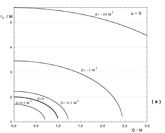
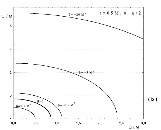
Figure 1: The dependence of the size of the horizon of black holes localized on a 3-brane in the Randall-Sundrum braneworld on the electric charge of the black holes for different values of their tidal charge $\,\beta\,.$ Figure (a) corresponds to a non-rotating black hole, while figure (b) is for a rotating black hole with $\,a=0.5M\,$and $\,\theta=\pi/2\,$.

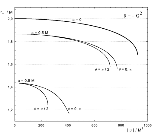
Figure 2: The dependence of the horizon radius of a rotating braneworld black hole in its equatorial plane $\,\theta=\pi/2\,$ and at poles $\,\theta=0\,,\,\pi\,$ on the absolute value of its tidal charge $\,\beta=-Q^{2}\,$ for given values of the rotation parameter $\,a=0\,,\,\,0.5M\,,\,\,0.9M\,.$

We have applied numerical calculations to analyze the largest roots of equation (63). The numerical results are plotted in Figs. 1(a,b) and Fig. 2. For the sake of certainty in all numerical calculations we have set the curvature radius of AdS $\,l=0.01M^{2}\,.$ In Fig. 1(a) the plots illustrate the dependence of the horizon radius on the electric charge of the black hole with vanishing rotation parameter $(\,a=0\,)$ and different values of the tidal charge $\,\beta=0\,,\,\,\pm 0.5M^{2}\,,\,-5M^{2}\,,\,\,-20M^{2}\,\,$. As expected, the size of the horizon is sensitive to the sign of tidal charge. We see that, in contrast to its positive values, the negative tidal charge has greatest effect of increasing the horizon radius, while the electric charge of the black hole opposes it. In all cases the horizon radius decreases with increasing electric charge and the critical values of the electric charge at which the horizon does exist are different for different values of $\,\beta\,.$ Fig. 1(b) involves the similar plots with the value of the rotation parameter $\,a=0.5M^{2}\,$ in the equatorial plane $(\,\theta=\pi/2\,).$ One sees that the effect of rotation of the black hole, just as that of electric charge, is to decrease the horizon radius.

Fig. 2 presents some results of the numerical analysis of the horizon radius for a particular value of the tidal charge $\,\beta=-Q^{2}\,.$ The plots reveal the different size of the horizon in different $\,\theta\,$-planes with increasing absolute value of the tidal charge. The effect becomes more significant with the growth of rotation parameter. We see that for given charge the horizon radius at poles $\,\theta=0\,\,,\,\pi\,$ is always greater than at $\,\theta=\pi/2\,$ . Furthermore, the critical absolute value of $\,\beta\,$ at which the horizon exist is also greater for $\,\theta=0\,\,,\,\pi\,.$

To conclude this section we note that the boundary of the ergosphere in metric (57)can be described in a usual manner, that is by the condition $\,g_{tt}=0\,$. This can be also written in the form

$$r^{2}-2Mr+\beta+Q^{2}+a^{2}\cos^{2}\theta+\frac{l^{2}Q^{4}}{8a^{4}\cos^{4}\theta}\left[2+\frac{r^{2}}{\Sigma}+\frac{3r}{a\cos\theta}\arctan\left(\frac{r}{a\cos\theta}\right)\right]=0\,\,.$$ (68)

The comparison of this equation with (63) shows that the ergosphere region always lies beyond the event horizon coinciding with it only at poles $\,\theta=0\,,\,\,\pi\,$.

V Geodesic motion

It is generally believed that in situations of astrophysical interest the electric charge of a Kerr black hole will quickly become negligible due to the neutralizing effect of an ionized medium surrounding the black hole. The same argument may remain true for a rotating black hole in the braneworld scenario, where charged particles can live only on the brane and their selective accretion by the black hole will significantly diminish its electric charge. However, in the latter case even without electric charge being present, the black hole may still have a tidal charge emerging as a pure geometrical effect from the bulk space dmpr . Therefore, the above argument does not apply to constraint the value of the tidal charge and it, in principle, may have its greatest effect on physical processes in the strong-gravity region around the black hole. To get some insights into this we shall now study the geodesic motion of test particles in the metric (35) of a rotating black hole with tidal charge .

We start with the Hamilton-Jacobi equation

$$h^{ij}\,\frac{\partial S}{\partial x^{i}}\,\frac{\partial S}{\partial x^{j}}+m^{2}=0,$$ (69)

where $m$ is the mass of a test particle. Following Carter’s result carter of the complete separability of this equation in the metric of a Kerr-Newman black hole in general relativity we can write the action in the form

$$S=-Et+L\phi+S_{r}(r)+S_{\theta}(\theta)\,,$$ (70)

where the conserved quantities $E$ and $L$ are the energy and the angular momentum of the test particle at infinity, respectively. Substituting it into equation (69) we obtain the two equations in the separable form

$$\Delta\left(\frac{dS_{r}}{dr}\right)^{2}-\frac{1}{\Delta}\,\left[(r^{2}+a^{2})E-a\,L\right]^{2}+m^{2}r^{2} = -\textsc{K}\,\,,$$ (71)

$$\left(\frac{dS_{\theta}}{d\theta}\right)^{2}+\left(aE\sin\theta-\frac{L}{\sin\theta}\right)^{2}+m^{2}a^{2}\cos^{2}\theta = \textsc{K}\,\,,$$ (72)

where  K  is a constant of separation. We shall restrict ourselves to geodesic motion in the equatorial plane $\,\theta=\pi/2\,$. Then using equations (71) and (72), along with the action(70), in the expression

$$\frac{dx^{i}}{d\lambda}=h^{ij}\,\frac{\partial S}{\partial x^{j}}\,\,,$$ (73)

where $\,\lambda=s/m\,$ is an affine parameter along the trajectory of the particle, we arrive at the following equations of motion

$$\Delta\,\frac{dt}{d\lambda} = \left(r^{2}+a^{2}+\frac{2Mr-\beta}{r^{2}}\,\,a^{2}\right)E-\frac{2Mr-\beta}{r^{2}}\,\,aL\,\,,$$

$$\Delta\,\frac{d\phi}{d\lambda} = \left(1-\frac{2Mr-\beta}{r^{2}}\right)L+\frac{2Mr-\beta}{r^{2}}\,\,aE\,\,,$$ (74)

and

$$r^{4}\,\left(\frac{dr}{d\lambda}\right)^{2}=V(E,L,r,a,\beta)\,\,,$$ (75)

where the effective potential of the radial motion is given by

$$V=\left[(r^{2}+a^{2})\,r^{2}+(2Mr-\beta)\,a^{2}\right]E^{2}-(r^{2}-2Mr+\beta)\,L^{2}$$

$$-2\,a(2Mr-\beta)\,EL-m^{2}r^{2}\Delta\,\,.$$ (76)

From the symmetry of the problem it follows that a simple example of the geodesic motion, the circular motion, occurs in the equatorial plane of the black hole. The energy and the angular momentum of the circular motion at some radius are determined by the simultaneous solution of the equations

$$V = 0\,\,,~{}~{}~{}~{}~{}~{}~{}~{}~{}~{}\frac{\partial V}{\partial r}=0\,\,.$$ (77)

Solving these equation yields

$$\frac{E}{m}=\frac{r^{2}-2Mr+\beta\pm a\,\sqrt{Mr-\beta}}{r\,\left[r^{2}-3Mr+2\beta\pm 2\,a\,\sqrt{Mr-\beta}\,\right]^{1/2}}\,\,\,,$$ (78)

$$\frac{L}{m}=\pm\,\frac{\sqrt{Mr-\beta}\left(r^{2}+a^{2}\mp 2\,a\,\sqrt{Mr-\beta}\right)\mp a\beta}{r\,\left[r^{2}-3Mr+2\beta\pm 2\,a\,\sqrt{Mr-\beta}\,\right]^{1/2}}\,\,\,.$$ (79)

Here and in the following the upper sign corresponds to the so-called direct orbits in which the particles are corotating $\,(L>0\,)$ with respect to the rotation of the black hole, while the lower sign applies to the retrograde, counterrotating $\,(L<0)\,$ motion of the particles.

From equation (78) it follows that the region of existence of the circular orbits extends from infinity up to the radius of the limiting photon orbit, which is determined by the condition

$$r^{2}-3Mr+2\beta\pm 2\,a\sqrt{Mr-\beta}=0\,\,.$$ (80)

It is evident that in the region of existence not all circular orbits are bound. The radius of the marginally bound orbits with $\,E^{2}=m^{2}\,$ is given by the largest root of the polynomial equation

$$Mr\left(4Mr-r^{2}-4\beta+a^{2}\right)+\beta\left(\beta-a^{2}\right)\pm\,2a\left(\beta-2Mr\right)\sqrt{Mr-\beta}=0\,\,.$$ (81)

The condition for stability of the circular motion is given by the inequality

$$\frac{\partial^{2}V}{\partial r^{2}}\leq 0\,\,,$$ (82)

where the case of equality corresponds to the marginally stable circular orbits. Next, substituting expressions (78) and (79) into (82) we obtain the equation governing the boundary of the marginally stable orbits

$$Mr\left(6Mr-r^{2}-9\beta+3\,a^{2}\right)+4\beta\left(\beta-a^{2}\right)\mp\,8a\left(Mr-\beta\right)^{3/2}=0\,\,.$$ (83)

We note that the similar equations of the form of (80), (81) and (83) for a circular geodesic motion in the equatorial plane of the Kerr-Newman black hole in general relativity were obtained a long time ago in dk . The numerical analysis of the boundaries of the equatorial circular orbits in the Kerr-Newman metric as functions of the rotation parameter and the electric charge of the black hole was given in alievg . In particular, it has been shown that the radius of the limiting photon orbit, as well as the radii of the innermost bound and the innermost stable circular orbits moves towards the event horizon with the growth of black hole’s electric charge both for direct and retrograde motions.

It is evident that in our case the positive tidal charge will play the same role in its effect on the circular orbits as the electric charge in the Kerr-Newman metric. However, as it has been emphasized in Sec.III, the case of negative tidal charge is physically more natural case on the brane and therefore, here we wish to know how the negative tidal charge affects the circular geodesics. For this purpose, we apply a numerical analysis to study the solutions of equations (80), (81) and (83). The numerical analysis shows that, regardless to the direct, or retrograde motions of the particles, the limiting radii for existence, bound and stability of the circular orbits enlarges from the event horizon as the absolute value of $\,\beta\,$ increases. In particular, for $\,\beta=-M^{2}\,$ and $\,a=0\,$ we find that the radii of the limiting photon and the last stable orbits are given as

$$r_{ph} \simeq 3.56M\,,~{}~{}~{}~{}~{}~{}r_{ms}\simeq 7.3M\,,$$ (84)

while the radius of the event horizon $\,r_{+}=(1+\sqrt{2})M\,.$ For a comparison we recall that for the same but positive value of the tidal charge, which at the same time is the limiting value of the charge in the Reissner-Nördstrom metric one finds

$$r_{ph} = 2M\,,~{}~{}~{}~{}~{}~{}r_{ms}=4M\,,~{}~{}~{}~{}~{}~{}r_{+}=M\,.$$ (85)

For these two cases it is also instructive to compare the binding energies per unit mass of a particle at the last stable circular orbits. Thus, for $\,\beta=-M^{2}\,$ using (78) we find that

$$E_{binding}=1-\frac{E}{m}\simeq 4.7\,\%\,\,,$$ (86)

in contrast to the binding energy $\,E_{binding}\simeq 8.1\,\%\,\,$ of a particle in the case of $\,\beta=M^{2}\,.$ We conclude that in the $\,\beta<0\,$ case the binding energy of a particle moving in the last stable circular orbits around a static black hole decreases in contrast to the $\,\beta>0\,$ case, where it increases attaining its maximum value for the limiting case of $\,\beta=M^{2}\,.$

For a rotating black hole with the negative tidal charge $\,\beta=-M^{2}\,$ and the rotation parameter $\,a=M\,,$ the numerical calculations for the direct motion give

$$r_{ph} \simeq 2.89M\,,~{}~{}~{}~{}~{}~{}r_{ms}\simeq 3.89M\,,~{}~{}~{}~{}~{}E_{binding}\simeq 9\,\%\,,$$ (87)

while, for the retrograde motion we obtain

$$r_{ph} \simeq 4.48M\,,~{}~{}~{}~{}~{}~{}r_{ms}\simeq 10.15M\,,~{}~{}~{}~{}~{}E_{binding}\simeq 3\,\%\,.$$ (88)

We recall that for this case the pertaining radius of the horizon radius $\,r_{+}=2M\,.$ In the meantime, the counterparts of these expressions bardeen for a maximally rotating black hole in general relativity $(\,a\rightarrow M\,,\,\,\,r_{+}\rightarrow M\,)$ are given by $\,r_{ph}\simeq M\,,~{}~{}r_{ms}\simeq M\,,~{}~{}E_{binding}\simeq 42\,\%\,$ for the direct orbit, and $\,r_{ph}\simeq 4M\,,~{}~{}r_{ms}\simeq 9M\,,~{}~{}E_{binding}\simeq 3.7\,\%\,$ for the retrograde orbit. We note that compared to the case of a maximally rotating black hole in general relativity for which only zero-electric charge is acceptable, the presence of negative tidal charge increases the radii of the marginally stable orbits in both direct and retrograde motions, thereby decreasing the corresponding binding energies. However, it should be emphasized that the value of the rotation parameter $\,a=M\,$ is not a limiting value for the braneworld black hole carrying negative tidal charge. For instance, for $\,\beta=-M^{2}\,$ it becomes $\,a=\sqrt{2}M\,.$ In this case, the radius of the horizon is $\,r_{+}=M\,$, and instead of the expressions (87) and (88) we have

$$r_{ph} \simeq M\,,~{}~{}~{}~{}~{}~{}r_{ms}\simeq M\,,~{}~{}~{}~{}~{}E_{binding}\simeq 46.5\,\%\,\,,$$ (89)

for the last direct circular orbit and

$$r_{ph} \simeq 4.82M\,,~{}~{}~{}~{}~{}~{}r_{ms}\simeq 11.25M\,,~{}~{}~{}~{}~{}E_{binding}\simeq 3\,\%\,,$$ (90)

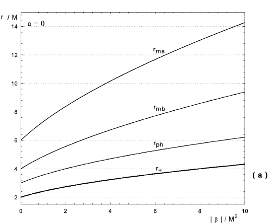
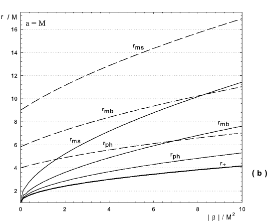
Figure 3: Radii of the event horizon, the limiting photon orbit, the marginally bound and the marginally stable circular orbits in the equatorial plane $(\,\theta=\pi/2\,)$ of a rotating black hole carrying a tidal charge. The curves illustrate the dependence of the radii on the absolute value of the tidal charge $(\,\beta<0\,)$ for given values of the rotation parameter $\,a=0\,$ (figure (a)) and $\,a=M\,$ (figure (b)). The solid curves correspond to direct orbits, whereas the dashed curves refer to retrograde orbits. The position of the horizon is indicated by the bold curve.

for the last retrograde one. In particular, from equation (89) we see that for the class of direct orbits, the negative tidal charge tends to increase (through increasing the limiting value of the rotation parameter compared to that of in general relativity) the efficiency of an accretion disc around a maximally rotating braneworld black hole. The details of the numerical results are plotted in Figs. 3(a,b) and 4(a,b) . In figure 3(a) for the $\,\beta<0\,$ case the curves display the growth of the horizon size, the radius of the limiting photon orbit, as well as the radii of the last bound and the last stable circular orbits with increasing absolute value of the tidal charge of a non-rotating black hole. For the same case of $\,\beta<0\,$, the figure 3 (b) plots the same curves for given non-zero value of black hole’s rotation parameter $\,a=M\,.$ We see that for all cases increasing the absolute value of the tidal charge appears to increase the radii of the limiting circular orbits.

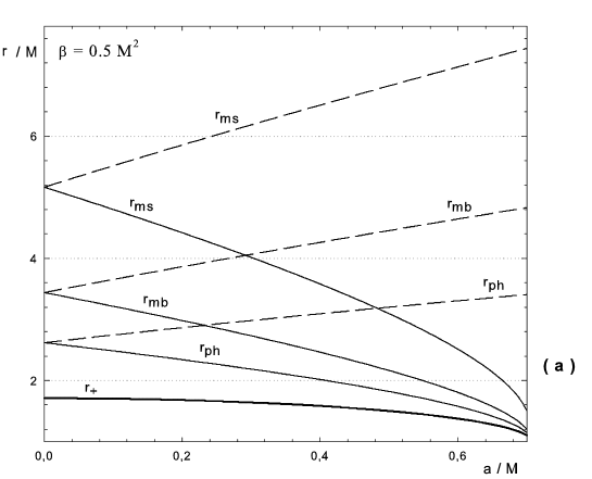
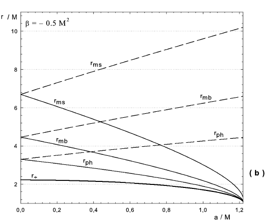
Figure 4: The positions of the event horizon, the limiting photon orbit , the marginally bound and the marginally stable circular orbits around a rotating black hole on the brane with the effects of the rotation parameter for given values of $\,\beta=\pm\,0.5M^{2}\,.$ The solid curves are for direct motions, whereas the dashed curves are for retrograde motions.

The curves of figure 4 (a,b) illustrate the dependence of the horizon size, the radius of the limiting photon orbit and the radii of the marginally bound and the marginally stable orbits on the rotation parameter of the black hole for given $\,\beta=\pm\,0.5M^{2}\,.$ The positive tidal charge acts to decrease the radii of circular orbits in both direct and retrograde motions, just as an electric charge in general relativity (Fig.4(a)). On the other hand, the negative tidal charge has its opposite effect of increasing the radii, regardless to a particular class of circular orbits (Fig. 4(b)). In both cases the effect of the rotation is to decrease the radii for direct orbits and to increase them for retrograde ones.

VI Conclusion

The exact bulk metrics that consistently describe the formation of black holes as endpoints of gravitational collapse of matter on a 3-brane in the Randal-Sundrum scenario have not been constructed yet. One of the attempts made in this direction is based on a specialization of the induced metrics on the brane and then solving the effective gravitational field equations for these metrics. The subsequent integration of the field equations into the bulk using the induced metrics as ”initial data” could provide the desired solutions for braneworld black holes. Following the similar line, in this paper we have specified a particular metric ansatz for rotating black holes localized on a 3-brane in the Randall-Sundrum braneworld . Namely, we have assumed that the metrics describing rotating black holes on the brane would admit the familiar Kerr-Schild form.

First, we have considered the case of an empty brane and solved the constraint equations on the brane, which together with the effective gravitational field equations on the brane form a closed set of equations for our Kerr-Schild ansatz. We have shown that the resulting metric is not in a usual Kerr form, instead it involves an extra non-trivial parameter which looks like to play exactly the same role as a Maxwell electric charge in the Kerr-Newman solution of general relativity. However, the extra parameter in our case has a pure geometrical origin and can be naturally interpreted as a tidal charge transmitting to the brane the gravitational imprints of the bulk space. It is interesting to note that, in contrast to the ”squared” electric charge in the Kerr-Newman metric, the tidal charge in the rotating black hole metric on the brane may take on both positive and negative values. Moreover, as it has been argued in a number of papers (see Refs. chrss , roy1 , sms2 ) that the case of negative tidal charge is physically more natural one, since it acts in the same direction as the negative cosmological constant to keep the gravitational field (the horizon of a black hole) around the brane.

We have also studied the effects of negative tidal charge on the horizon structure and the ergosphere of the rotating black hole on the empty brane. In particular, we have found that the negative tidal charge may provide a mechanism for spinning up the black hole to the value of its rotation parameter which is greater than its mass. This is not allowed in the framework of general relativity. The negative tidal charge extends the boundary of the ergosphere, thereby making the rotating braneworld black hole a more energetic object with respect to the extraction of its rotational energy.

Next, we have turned to the case of non-empty brane, assuming the presence of a Maxwell field on it. In this case a rotating black hole on the brane, in addition to its tidal charge, would also carry an electric charge of the Maxwell field. Using again the Kerr-Schild ansatz for the induced metric on the brane we have presented a new solution describing such a black hole . It turned out that for a rapid enough rotation the composite effects of the black hole rotational dynamics and the ”squared” energy-momentum tensor on the brane distort the geometry of the black hole in such a way that it has a differentiated horizon structure at each fixed $\,\theta$-plane. In other words, the horizon depends on the values of $\,\theta$-angle, and therefore the horizon structure of the black hole can be thought of as composed of non-uniformly rotating null circles. We have also numerically solved the corresponding equation governing the radii of the circles. In particular, we have shown that for given special values of the charges the radius of the horizon at poles $(\,\theta\,=0\,,\,\pi)$ is greater than that of in the equatorial plane $(\,\theta=\,\pi/2)\,.$ The difference becomes more significant with the growth of black hole’s rotation parameter.

Finally, we have investigated the circular geodesic motion of test particles in the equatorial plane of a rotating braneworld black hole carrying a tidal charge. We have found that the negative tidal charge has its greatest effect in increasing the radius of the horizon, as well as the radii of existence, boundedness and stability for the innermost circular orbits, regardless to the direct, or retrograde classes of the orbits.

We would like to note that it is not clear that the Kerr-Schild ansatz for the induced metrics on the brane we have used in this paper to describe rotating braneworld black hole is indeed fulfilled by an exact bulk metric. Nevertheless, we believe that our approach even without constructing exact bulk metrics gives significant insight into the physics of rotating black holes localized on a 3-brane in the Randall-Sundrum scenario. In the context of possible observational signatures of the rotating black holes with tidal charge it would be interesting to study their gravitational lensing effects. Certainly, it would be also very interesting to explore the evolution into the bulk space of the black hole solutions given in this paper using both analytical and numerical calculations.

VII Acknowledgment

We would like to thank Roy Maartens for useful discussions at an early stage of this work.

References

- (1) N. Arkani-Hamed, S. Dimopoulos, and G. Dvali, Phys. Lett. B 429, 263 (1998).
- (2) I. Antoniadis, N. Arkani-Hamed, S. Dimopoulos, and G. Dvali, Phys. Lett. B 436, 257 (1998).
- (3) L. Randall and R. Sundrum, Phys. Rev. Lett. 83, 3370 (1999) .
- (4) L. Randall and R. Sundrum, Phys. Rev. Lett. 83, 4690 (1999) .
- (5) V. A. Rubakov and M. E. Shaposhnikov, Phys. Lett. B 125, 136 (1983); K. Akama, Lecture Notes in Physics, 176, 267 (1982) hep-th/0001113; M. Visser, Phys. Lett. B 159, 22 (1985); M. Gogberashvili, Mod. Phys. Lett. A 14, 2025 (1999) .
- (6) R. Maartens, Living Rev. Rel. 7, 7 (2004) .
- (7) P. Kanti, Int. J. Mod. Phys. A 19, 4899 (2004) .
- (8) G. Gabadadze, ICTP Lectures on Large Extra Dimensions hep-ph/0308112 .
- (9) M. Cavaglia, Int. J. Mod. Phys. A 18, 1843 (2003) .
- (10) V. Rubakov, Phys. Usp. 44, 871 (2001); Usp. Fiz. Nauk 171, 913 (2001) .
- (11) R. Emparan, M. Masip, and R. Rattazzi, Phys. Rev. D 65, 064023 (2002) .
- (12) S. B. Giddings and S. Thomas, Phys. Rev. D 65, 056010 (2002) .
- (13) S. Dimopoulos and G. Landsberg, Phys. Rev. Lett. 87, 161602 (2001) .
- (14) J. Garriga and T. Tanaka, Phys. Rev. Lett. 84, 2778 (2000) .
- (15) S. B. Giddings, E. Katz and L. Randall, J. High Energy Phys. 0003, 23 (2000) .
- (16) T. Shiromizu, K. Maeda, and M. Sasaki, Phys. Rev. D 62, 024012 (2000) .
- (17) F. R. Tangherlini, Nuovo Cimento 77, 636 (1963) .
- (18) R. C. Myers and M. J. Perry, Ann. Phys. (N.Y.) 172, 304 (1986) .
- (19) V. Frolov and D. Stojkovic, Phys. Rev. D 67, 084004 (2003).
- (20) V. Frolov and D. Stojkovic, Phys. Rev. D 68, 064011 (2003).
- (21) R. Emparan and R. C. Myers, J. High Energy Phys. 0309, 025 (2003).
- (22) A. N. Aliev and V. Frolov, Phys. Rev. D 69, 084022 (2004).
- (23) D. Stojkovic, Phys. Rev. Lett. 94, 011603 (2005).
- (24) M. Sakaguchi and Yukinori Yasui, (2005) hep-th/0502182 .
- (25) H. Kudoh, T. Tanaka and T. Nakamura, Phys. Rev. D 68, 024035 (2003) .
- (26) R. Emparan, G. T. Horowitz and R. C. Myers, J. High Energy Phys. 0001, 007 (2000) .
- (27) R. Emparan, G. T. Horowitz and R. C. Myers, J. High Energy Phys. 0001, 021 (2000) .
- (28) A. Chamblin, S. W. Hawking and H. S. Reall, Phys. Rev. D 61 065007 (2000) .
- (29) R. Gregory and R. Laflamme, Phys. Rev. Lett. 70, 2837 (1993); R. Gregory, Class. Quant. Grav. 17, L125 (2000) .
- (30) G. T. Horowitz and K. Maeda, Phys. Rev. Lett. 87, 131301 (2001) .
- (31) M. S. Modgil, S. Panda and G. Sengupta, Mod. Phys. Lett. A 17, 1479 (2002) .
- (32) S. Nojiri, O. Obregon, S. D. Odintsov and S. Ogushi, Phys. Rev. D 62, 064017, (2000).
- (33) N. Dadhich, R. Maartens, P. Papadopoulos and V. Rezania, Phys. Lett. B 487, 1 (2000) .
- (34) C. Germani and R. Maartens, Phys. Rev. D 64, 124010 (2001) .
- (35) A. Chamblin, H. S. Reall, H. A. Shinkai and T. Shiromizu, Phys. Rev. D 63, 064015 (2001).
- (36) R. Casadio, A. Fabbri and L. Mazzacurati, Phys. Rev. D 65, 084040 (2002).
- (37) P. Kanti and K. Tamvakis, Phys. Rev. D 65, 084010 (2002) .
- (38) R. Gregory, R. Whisker, K. Beckwith and C. Done, J. Cosmology and Astropart. Phys. 10, 013 (2004).
- (39) R. Whisker, (2004) astro-ph/0411786 .
- (40) A. N. Aliev and A. E. Gumrukcuoglu, Class. Quant. Grav. 21, 5081 (2004).
- (41) R. Arnowitt, S. Deser, and C.W. Misner, In Gravitation: an introduction to current research, L. Witten, ed. Wiley, New York, p.227 (1962); gr-qc/0405109.
- (42) E. Poisson, A Relativist’s Toolkit: The Mathematics of Black Hole Mechanics, Cambridge University Press (2004) .
- (43) W. Israel, Nuovo Cimento 44B, 1 (1966); Errata-ibid 48B, 463 (1967) .
- (44) P. S. Apostolopoulos and N. Tetradis, Phys. Rev. D 71, 043506 (2005) .
- (45) M. Minamitsuji, M. Sasaki and D. Langlois, (2005) gr-gc/0501086 .
- (46) R. P. Kerr and A. Schild, Proc. Symp. Appl. Math. 17,199 (1965) .
- (47) R. Maartens, Phys. Rev. D 62, 084023 (2000) .
- (48) M. Sasaki, T. Shiromizu, K. Maeda , Phys. Rev. D 62, 024008 (2000) .
- (49) B. Carter in General Relativity, An Einstein centenary survey edited by S.W. Hawking and W. Israel, Cambridge University Press, Cambridge, England, 1979 .
- (50) B. Carter, Phys. Rev. 174, 1559 (1968) .
- (51) N. Dadhich and P. P. Kale, J. Math. Phys. 18, 1727 (1977) .
- (52) A. N. Aliev and D. V. Gal’tsov, Gen. Relat. Gravit. 13, 899 (1981) .
- (53) J. M. Bardeen, W. H. Press and S. A. Teukolsky, Astrophys. J. 178, 347 (1972) .