Hydrogen-atom spectrum under a minimal-length hypothesis

Abstract

The energy spectrum of the Coulomb potential with minimal length commutation relations $[X_{i},P_{j}]=i\hbar\{\delta_{ij}(1+\beta P^{2})+\beta^{\prime}P_{i}P_{j}\}$ is determined both numerically and perturbatively for arbitrary values of $\beta^{\prime}/\beta$ and angular momenta $\ell$. The constraint on the minimal length scale from precision hydrogen spectroscopy data is of order of a few GeV^-1, weaker than previously claimed.

Quantum gravity incorporates Newton’s constant as a dimensional parameter that could manifest itself as a minimal length in the system. Recent string theoretic considerations suggest that this length scale might imply an ultraviolet-infrared (UV-IR) correspondence, contrary to the normal perceptions on momentum and spatial separations. Large momenta are now directly tied to large spatial dimensions, which then implies the existence of a minimal length. Earlier studies have focused upon its amelioration of ultraviolet divergences earlyQM , but did not take into full account the UV-IR correspondence.

There are various ways of implementing such an idea, but the simplest is to suppose that coordinates no longer commute in $D$-dimensional space. This, in turn, leads to a deformation of the canonical commutation relations. In our previous works, we adopted the equivalent hypothesis that the fundamental commutation relations between position and momentum are no longer constant multiples of the identity. In this paper, we report on constraints on the minimal length hypothesis from precision measurements on hydrogenic atoms. This system has a potential that is singular at the origin, and is therefore particularly sensitive to whether there is a fundamental minimal length. Considerations based upon higher-dimensional theories suggest that such lengths may be large LXD .

To set the context, we note that if in one dimension we have

$$[\hat{X},\hat{P}]=i\hbar(1+\beta\hat{P}^{2}),$$ (1)

where $\beta$ is a small parameter, then the resulting uncertainty relation $(\Delta X)(\Delta P)\geq i\hbar\{1+\beta(\Delta P)^{2}\}$ exhibits a form of the UV-IR correspondence, and gives as minimal length $\Delta X\geq\hbar\sqrt{\beta}$ Kempf .

We had examined the harmonic oscillator system under this hypothesis in HO , but no real constraint can be obtained on the minimal length, presumably because of the softness of the potential at the origin. An interesting approach is to take the classical limit $\hbar\to 0$ of the commutation relations; it yields an unbelievably strong bound, but its robustness might be questioned ClassLim .

We will work in arbitrary $D>1$ dimensions, where (1) takes the tensorial form

$$[\hat{X}_{i},\hat{P}_{j}]=i\hbar\{\delta_{ij}(1+\beta\hat{P}^{2})+\beta^{\prime}\hat{P}_{i}\hat{P}_{j}\},$$ (2)

which, assuming that the momenta commute $[\hat{P}_{i},\hat{P}_{j}]=0,$ leads via the Jacobi identity to the nontrivial position commutation relations

$$[\hat{X}_{i},\hat{X}_{j}]=i\hbar\,\frac{(2\beta-\beta^{\prime})+(2\beta+\beta^{\prime})\beta\hat{P}^{2}}{(1+\beta\hat{P}^{2})}(\hat{P}_{i}\hat{X}_{j}-\hat{P}_{j}\hat{X}_{i}).$$

The position and momentum operators can be represented by

$$\hat{X}_{i}=(1+\beta\hat{p}^{2})\hat{x}_{i}+\beta^{\prime}\hat{p}_{i}\hat{p}_{j}\hat{x}_{j},\qquad\hat{P}_{i}=\hat{p}_{i},$$ (3)

where the operators $\hat{x}_{i}$ and $\hat{p}_{j}$ satisfy the canonical commutation relations $[\hat{x}_{i},\hat{p}_{j}]=i\hbar\delta_{ij}.$ The simplest representation is momentum diagonal,

$$\hat{x}_{i}=i\hbar\frac{\partial}{\partial p_{i}},\qquad\hat{p}_{i}=p_{i}.$$ (4)

In this representation the eigenvalue equation for the distance squared operator $\hat{R}^{2}=\hat{X}_{i}\hat{X}_{i}$ can be solved exactly. With

$$z=\frac{(\beta+\beta^{\prime})p^{2}-1}{(\beta+\beta^{\prime})p^{2}+1},$$ (5)

the eigenvalues ${r_{n\ell}^{2}}=\hbar^{2}(\beta+\beta^{\prime})\rho_{n\ell}^{2}$ and eigenfunctions $R_{n\ell}$ are given by (see HO for details)

$$\rho_{n\ell}^{2}=(2n+a+b+1)^{2}-(1-\eta)^{2}\left(L^{2}+\dfrac{(D-1)^{2}}{4}\right),$$

$$R_{n\ell}(z)\propto(\beta+\beta^{\prime})^{D/4}\left.\left(\frac{1-z}{2}\right)\!\!\right.^{\lambda/2}\left.\left(\frac{1+z}{2}\right)\!\!\right.^{\ell/2}P_{n}^{(a,b)}(z),$$

where $P_{n}^{(a,b)}(z)$ are the Jacobi polynomials and

$$\eta =\frac{\beta}{\beta+\beta^{\prime}},\qquad a =\sqrt{\frac{[1+(D-1)\eta]^{2}}{4}+\eta^{2}L^{2}},$$

$$b =\frac{D}{2}+\ell-1,\qquad \lambda =\frac{1+(D-1)\eta}{2}+a.$$ (6)

Having diagonalized $\hat{R}^{2}$, one can express the action of the $\hat{R}^{-1}$ operator on any function of definite angular momentum $\Psi(z)=\sum_{n=0}^{\infty}f_{n}R_{n\ell}(z).$ In particular, the Schrödinger equation for the Coulomb problem, $\left(\hat{P}^{2}/2m-k/\hat{R}\right)\Psi(p)=E\,\Psi(p),$ can be rewritten in the variable $z$ as

$$\sum_{n=0}^{\infty}f_{n}\left[\left(\frac{1+z}{1-z}\right)+\epsilon-\frac{2\xi}{\rho_{n\ell}}\right]R_{n\ell}(z)=0,$$ (7)

$\xi=\Delta x_{\min}/a_{0}$ being the ratio of the minimal length $\Delta x_{\mathrm{min}}=\hbar\sqrt{\beta+\beta^{\prime}}$ to the Bohr radius $a_{0}=1/km$, and $\epsilon=\xi^{2}(E/E_{0})$ the energy in units of the usual ground-state energy $E_{0}=-1/2a_{0}^{2}m$ times $\xi^{2}$.

Using the recursion relation for Jacobi polynomials as well as the orthogonality of the distance eigenfunctions $R_{n\ell}$, the Schrödinger equation is equivalent to a recursion relation for the expansion coefficients,

$$f_{n+1}s_{n+1}\hat{a}_{n}+f_{n}t_{n}+f_{n-1}s_{n-1}\hat{a}_{n-1}=0,$$ (8)

with $f_{-1}=0$, $s_{n}=1-\epsilon+2\xi/\rho_{n\ell}$,

$$t_{n} =(2-s_{n})-s_{n}\frac{a^{2}-b^{2}}{(2n+a+b)(2n+a+b+2)},$$

and

$$\hat{a}_{n} =-\frac{2}{(2n+a+b+2)}$$

$$\quad\times\sqrt{\frac{(n+1)(n+a+1)(n+b+1)(n+a+b+1)}{(2n+a+b+1)(2n+a+b+3)}}.$$

For a normalizable solution we must have $\langle\Psi|\Psi\rangle=\sum_{n=0}^{\infty}f_{n}^{2}(\epsilon)$ finite, thus $f_{n}$ should converge to zero. A closed-form expression for this sequence cannot be determined. One can observe though that for large $n$ it asymptotically approaches

$$f_{n}\sim C_{+}\lambda_{+}^{n}+C_{-}\lambda_{-}^{n}\qquad\text{with }\lambda_{\pm}=\frac{1\pm\sqrt{\epsilon}}{1\mp\sqrt{\epsilon}},$$ (9)

$C_{\pm}$ being constants that depend on the minimal length through $\xi$ and the energy eigenvalues through $\epsilon$. This allows one to determine numerically the Coulomb spectrum, by imposing $C_{+}=0$.

As an independent check, we used two different algorithms. First, for fixed minimal length $\xi$, we imposed $f_{n+1}/f_{n}=\lambda_{-}$ for sufficiently large $n$ and scanned for the values of $\epsilon$ for which the recursion (8) gives $f_{-1}=0$. The contents following (5), and concluding with the first algorithm just described, represent results in unpublished work of Joseph Slawny. We thank him for making these available to us prior to publication.

The second algorithm is more direct: for a given minimal length $\xi$, we determined the values $\epsilon$ for which $f_{n}$ converges to 0. The subtlety is that $C_{+}$ will never be represented internally as exactly zero, and the term corresponding to it will eventually dominate our sequence. One can still identify the energy eigenvalues from the sign switch which occurs in $C_{+}$ and correspondingly in the large-$n$ behavior of $f_{n}$.

The algorithms yield consistent results, sampled in Fig. 1.

Figure 1: Plot of energy eigenvalues of the Coulomb potential in units of the regular ground-state energy as a function of the minimal length in units of the Bohr radius $\xi=\hbar\sqrt{\beta+\beta^{\prime}}/a_{0}$. For principal quantum numbers $n=1,2,3$, two extreme cases are represented: $\beta^{\prime}=0$ (thick lines) and $\beta=0$ (thin lines). Continuous line, $\ell=0$; dotted line, $\ell=1$; dash-dotted line, $\ell=2$.

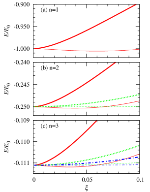
We can see that the degeneracy among different angular momentum states is lifted: higher-$\ell$ states get smaller corrections. The only exceptions are the $S$ states for $\beta^{\prime}>2\beta$ and $D=3$. These states start out with the lowest, negative correction for small $\xi$, but cross the higher-angular-momentum levels as $\xi$ increases. Another important remark, expected but not readily transparent in the representation used, is that the energy values converge to the usual result in the limit when the minimal length is taken to zero.

In order to get better insight into the observed behavior one can take another approach. This is also needed because for the very small values of the minimal length that interest us, i.e., several orders of magnitude below the Bohr radius, the numerical convergence becomes very slow and prone to rounding errors.

As mentioned before, the choice of momentum representation, while convenient, is not necessary. In relation (3) one can use the “pseudoposition” representation

$$\hat{x}_{i}=x_{i},\qquad\hat{p}_{i}=\frac{\hbar}{i}\frac{\partial}{\partial x_{i}},$$ (10)

in which the position operators $\hat{X}_{i}$ are not diagonal, except for the limit $\beta=\beta^{\prime}=0$. In this representation one can treat the $\beta$- and $\beta^{\prime}$-dependent terms as small, and use perturbation theory to deduce the corrections to the energy spectrum.

The operator $\hat{R}^{2}$ can be written as

$$\hat{R}^{2}=\hat{r}^{2}+\xi^{2}(\hat{R}^{2})_{\xi^{2}}+\xi^{4}(\hat{R}^{2})_{\xi^{4}},$$ (11)

where the first-order correction acts on the radial part of the wave-function through

$$\frac{(\hat{R}^{2})_{\xi^{2}}}{a_{0}^{2}} =-2\rho^{2}\frac{\partial^{2}}{\partial\rho^{2}}+[\eta(D-1)-3(D+1)]\rho\frac{\partial}{\partial\rho}$$

$$\quad+\eta(2L^{2}+D^{2}-D)-D(D+1),$$ (12)

with $\rho=r/a_{0}$ and $L^{2}=\ell(\ell+D-1)$.

In the expansion of the inverse distance $\hat{R}^{-1}=\hat{r}^{-1}+\xi^{2}(\hat{R}^{-1})_{\xi^{2}}+O(\xi^{4}),$ we expect on dimensional grounds that the first-order correction is a linear combination of terms of form $(1/\rho)\partial_{\rho\rho},(1/\rho^{2})\partial_{\rho}$, and $1/\rho^{3}$. Indeed, substituting this form into $\hat{R}^{-1}\hat{R}^{2}\hat{R}^{-1}=\hat{1}$ determines uniquely

$$\frac{(\hat{R}^{-1})_{\xi^{2}}}{a_{0}^{-1}} =\frac{[(2D-5)-\eta(2D-3)](D-1)-4\eta L^{2}}{4\rho^{3}}$$

$$\quad+\frac{(3-\eta)(D-1)}{2\rho^{2}}\frac{\partial}{\partial\rho}+\frac{1}{\rho}\frac{\partial^{2}}{\partial\rho^{2}}.$$ (13)

Thus, expressing the expectation value $\left<(1/\rho)\partial_{\rho\rho}\right>$ through the Schrödinger equation and $\left<(1/\rho^{2})\partial_{\rho}\right>$ in terms of $\left<1/\rho^{3}\right>$, the first-order corrections to the energy eigenvalues can be written as

$$\frac{\xi^{2}}{a_{0}^{2}m}\left\{\left[\frac{(D-1)(3\eta-1)}{4}-\bar{\ell}(\bar{\ell}+1)(1-\eta)\right]\!\Bigl{<}\frac{1}{\rho^{3}}\Bigr{>}\right.\\ \left.+2\Bigl{<}\frac{1}{\rho^{2}}\Bigr{>}-\frac{1}{\bar{n}^{2}}\Bigl{<}\frac{1}{\rho}\Bigr{>}-\left.\frac{(D-1)(1-\eta)\rho^{D-3}\!}{2}[\Pi_{n\ell}(\rho)]^{2}\right|_{0}^{\infty}\right\}\!,\\$$ (14)

where $\bar{n}=n+\frac{D-3}{2}$, $\bar{\ell}=\ell+\frac{D-3}{2}$, and $\Pi_{n\ell}(\rho)$ is the unperturbed Coulomb radial wave-function.

A note of caution is needed here. While the expansion is apparently in $\xi^{2}$, a quick calculation of higher-order terms confirms what is expected on dimensional grounds, namely, that the expansion parameter is $\beta/r^{2}=\xi^{2}/\rho^{2}$. The $\xi$-quartic part in the expansion (11) of $\hat{R}^{2}$ contains terms of the type $\xi^{4}/\rho^{2}$ and $(\xi^{4}/\rho)\partial_{\rho}$. Therefore, the approximation (Hydrogen-atom spectrum under a minimal-length hypothesis) for $\hat{R}^{-1}$ is no longer good for $\rho\lesssim\xi$. In particular, in the actual operator $\hat{R}^{-1}$ there is no singularity at the origin.

Let us estimate the error. The largest discrepancy between (LABEL:ExpVal) and the actual value comes from the expectation value of $1/\rho^{3}$ calculated over the interval $[0,\rho_{c}\xi]$ on which the approximation (Hydrogen-atom spectrum under a minimal-length hypothesis) breaks down, where $\rho_{c}\equiv r_{c}/a_{0}\sim 1$. For an angular momentum state $\ell$, this is of the order

$$\xi^{2}\int_{0}^{r_{c}\xi}\frac{R_{n\ell}^{2}(r)}{r^{3}}r^{D-1}dr\sim\xi^{2}\int_{0}^{r_{c}\xi}r^{2\ell+D-4}dr\\ \sim\xi^{2\ell+D-1},\qquad\text{for $\ell>0$ or $D>3$.}$$ (15)

For $D>3$ or $\ell\neq 0$, this contributes only a higher-order term; thus it is safe to use (LABEL:ExpVal), and we finally arrive at

$$\frac{\Delta E_{n\ell}}{E_{0}}=\frac{2\xi^{2}}{\bar{n}^{3}}\left[\frac{(D-1)\left(3\eta-1\right)}{4\bar{\ell}(\bar{\ell}+1)(\bar{\ell}+\frac{1}{2})}+\frac{\eta+1}{\bar{\ell}+\frac{1}{2}}-\frac{1}{\bar{n}}\right].$$ (16)

This expression generalizes the result of Ref. Brau for arbitrary $\eta$ and $D$. For the particular case $D=3$ and $\eta=1/3$ (i.e., $\beta^{\prime}=2\beta$) it reduces to the one obtained there. Moreover, it is in excellent agreement with our numerical results.

Figure 2: Comparison of different results for (a) 2$P$ states with $\eta=0,1$ and (b), (c) 1$S$ states with $\eta=0,1/3,1$. Solid lines, numeric result; dotted lines, perturbative result; dash-dotted lines, Ref. Brau ; double-dashed lines, Ref. AY . The perturbative expression is given for (a) by (16) and for (b), (c) by formula (17), with the coefficient $C$ chosen such that it agrees with the numerics at $\xi^{2}=10^{-6}$.

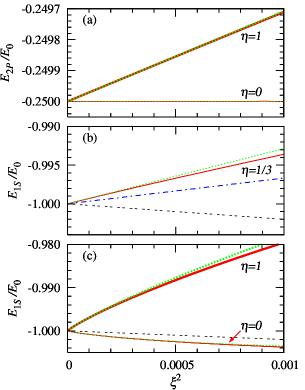
[See Fig. 2(a) for the case of the 2$P$ level.]

When $\ell=0$ and $D=3$, the integral (15) is infinite. We can use only the part of (Hydrogen-atom spectrum under a minimal-length hypothesis) that can be trusted, i.e., we have to cut off the expectation value integral $\left<1/\rho^{3}\right>$ at $\rho=\rho_{c}\xi$. The leading-order terms are

$$\frac{\Delta E_{n\ell}}{E_{0}}=\frac{4(3\eta-1)}{n^{3}}\xi^{2}E_{1}(\rho_{c}\xi)+C\xi^{2}+O(\xi^{3}),$$ (17)

where $E_{1}(\rho_{c}\xi)=-\ln\xi-(\gamma+\ln\rho_{c})+O(\xi)$ is the exponential integral function. The coefficient of the $\xi^{2}$ term gets contributions from several parts. First, there are the remaining terms in (LABEL:ExpVal). Second, the actual value of $\hat{R}^{-1}$ is bounded on the interval $[0,\rho_{c}\xi]$, so by cutting off the integral at $\rho_{c}\xi$ we are neglecting another term of order $\xi^{2}$. Lastly, the exact choice of the cutoff value $\rho_{c}$ contributes another $\xi^{2}$ term. Because we do not know the exact form of $\hat{R}^{-1}$, we cannot calculate analytically the second of these contributions. When needed, $C$ can be determined numerically, by fitting relation (17) to the numerical results at a sufficiently low value of $\xi^{2}$.

When compared to the numerical results, the behavior of the energy as a function of minimal length is nicely reproduced in Figs. 2(b) and 2(c). Our results disagree with Ref. Brau . The difference is well explained by the neglect there of all but linear terms in $\beta$. These terms critically affect the small-$r$ behavior of $\hat{R}^{-1}$, and cannot be neglected. Reference AY arrives at a different expression, which is independent of $\eta$. However, we could neither account for the discrepancy nor reproduce those results.

We can finally set out to determine the constraint on the minimal length $\Delta x_{\min}$ from precision hydrogen spectroscopy. A naive estimate, obtained by imposing that the corrections are smaller than the experimental error on the value of the hydrogen 1$S$-2$S$ splitting, gives $\Delta x_{\min}\gtrsim 300$ GeV (cf. Brau ; AY ). Unfortunately, this estimate would be correct only if the measured value of the physical observable agreed with the theoretical prediction and the main source of error were the experimental one. This is certainly not the case for the 1$S$-2$S$ splitting in hydrogen: known to 1.8 parts in $10^{14}$, it is one of the most precisely measured quantities today and is considered a de facto standard 1S2S . The value of the Rydberg constant is determined using this measurement as an input, and thus the theoretical uncertainty is orders of magnitude above the experimental one.

A better estimate is obtained by including contributions of the (hypothetical) minimal length in the Lamb shifts. The strongest constraint is expected from the 1$S$ Lamb shift, being the one determined most precisely and getting the largest correction. The measured 1$S$ state hydrogen Lamb shift of $L_{1S}^{\text{expt}}=8172.837(22)$ MHz 1Sexp is larger than today’s best theoretical prediction $L_{1S}^{\text{theor}}=8172.731(40)$ MHz 1Stheo by about 5$\sigma$ experimental uncertainty.

If we attribute the discrepancy entirely to the minimal length correction to the 1$S$ state, the bound as a function of $\eta$, obtained using the first two terms in (17), is shown in

Figure 3: Constraint on the minimal length obtained as a function of $\eta$, including the two highest-order terms (continuous line) and just the leading-order term (dash-dotted line).

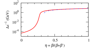
Fig. 3. It is 1.75 GeV for $\eta=1/3$ and increases to 6.87 GeV for $\eta=1$. Below $\eta=1/3$, the constraint relaxes rapidly. Indeed, in this case the leading-order term in (17) is negative, and only the contribution from the next term can account for the observed difference. As a comparison, including only the leading term, we can obtain a bound only for $\eta>1/3$, with consistent results for $\eta\gtrsim 0.5$.

We should point out that the theoretical Lamb shift predictions are somewhat frail because of the uncertainties in the proton charge radius 2Ptheo . These are the same order of magnitude as the ones discussed here; thus one should consider the values in Fig. 3 rather as upper limits for the minimal length. There is also the possibility of using muonium spectroscopy, but the current limits are still weak for our purposes. Details and other implications for QED are under investigation.