Conservation of Helicity and $SU(2)$ Symmetry in First Order Scattering

Abstract

The structure of the spin interaction operator (SI) ( the interaction that remains after space variables are integrated out) in the first order S-matrix element of the elastic scattering of a Dirac particle in a general helicity-conserving vector potential is investigated.It is shown that the conservation of helicity dictates a specific form of the SI regardless of the explicit form of the vector potential. This SI closes the $SU(2)$ algebra with other two operators in the spin space of the particle. The directions of the momentum transfer vector and the vector bisecting the scattering angle seem to define some sort of ”intrinsic” axes at this order that act as some symmetry axes for the whole spin dynamics . The conservation of helicity at this order can be formulated as the invariance of the component of the helicity of the particle along the bisector of the scattering angle in the transition.

I Introduction

It is well-known that the helicity of a Dirac particle is conserved given that there is no electric field acting on the particle J.J.Sakurai (1967). Indeed, the Heisenberg equation of motion for the helicity operator $\mathbf{\Sigma}.\mathbf{\Pi}$ where $\mathbf{\Pi}=(\mathbf{p}-e\mathbf{A})$ is the mechanical momentum of the particle reads ($\hbar=c=1$):

$$[\mathbf{\Sigma}.\mathbf{\Pi},H]=e\mathbf{\Sigma}\cdot\mathbf{E}$$ (1)

Here, $H=H_{0}+H_{\mathrm{int}}$, with

$$H_{0}=\bm{\alpha}\cdot\mathbf{p}+\beta m,$$ (2)

and

$$H_{\mathrm{int}}=eA_{0}-e\bm{\alpha}\cdot\mathbf{A},$$ (3)

$e$ is the charge of the particle, ${\alpha}_{i}=\beta\gamma_{i}$ and $\beta=\gamma_{4}$. The $\gamma$’s are the Dirac matrices: $\{\gamma_{\mu},\gamma_{\nu}\}=2g_{\mu\nu}$. Thus, in the absence of an electric field $\mathbf{E}$ helicity is conserved. In physical terms, conservation of helicity is described as the invariance of the component of the spin of the particle along its momentum. In the perturbative expansion of a helicity-conserving theory, helicity is conserved at each order of the perturbation series . For example, in the first order S-matrix element of the elastic scattering of a particle in some helicity-conserving vector potential, the conservation of helicity manifests itself through the fact that if the incident particle is in an eigen state of the operator $\mathbf{\Sigma}.\mathbf{\hat{p}}_{i}$ ($\mathbf{\hat{p}}_{i}\equiv\frac{\mathbf{p}_{i}}{|\mathbf{p}_{i}|}$) then the interaction will map it onto an eigenstate of $\mathbf{\Sigma}.\mathbf{\hat{p}}_{f}$ with the same eigenvalue J.J.Sakurai (1967) ( $\mathbf{p}_{i}$ and $\mathbf{p}_{f}$ are the incident and outgoing momenta, respectively). We can view this as if the interaction itself rotates the spin of the particle with the same angle $\theta$ with which it deviates the incident momentum so that the spin projection along the momentum is conserved in the transition. This work focuses on the conservation of helicity at this order and attempts to investigate the structure and properties of the spin interaction operator (SI) - the interaction operator that remains in the first order S-matrix of the scattering of a single Dirac particle after integrating out the space degrees of freedom- for a general helicity-conserving vector potentials. It will be shown that conservation of helicity at this order demands that this SI has a specific form regardless of the explicit form of the vector potential.As a concrete example, the Aharonov-Bohm (AB) potential Y.Aharonov and D.Bohm (1959) treated in an earlier work A.Albeed and M.S.Shikakhwa (2004) will be considered .

II Effective Spin Interaction

Consider a Dirac particle in a given magnetic field whose vector potential is the static vector function $\mathbf{A\mathbf{(}x)}$ and such that there is no scalar potential. The first order S-matrix element for the elastic scattering of a particle in this potential is :

$$S_{fi}^{(1)}=i\int{d^{4}x\,\bar{\psi}_{f}\left(x\right)\left(e\mathbf{\gamma}\cdot\mathbf{A}\right)\psi_{i}\left(x\right)}.$$ (4)

Carrying out the time integral,we get this as

$$S_{fi}^{(1)}=-2\pi e|N|^{2}\delta(E_{f}-E_{i})u^{\dagger}_{f}\left(p_{f},s_{f}\right)\left(\int{d^{3}x\,e^{i\left(\mathbf{p}_{f}-\mathbf{p}_{i}\right)\cdot\mathbf{x}}\left(\mathbf{\alpha}\cdot\mathbf{A}\right)}\right)u_{i}\left(p_{i},s_{i}\right).$$ (5)

which can be casted in the form

$$S_{fi}^{(1)}=-2\pi e|N|^{2}\delta(E_{f}-E_{i})u^{\dagger}_{f}\left(p_{f},s_{f}\right)\left(\mathbf{\alpha}\cdot\mathbf{A}(\mathbf{q})\right)u_{i}\left(p_{i},s_{i}\right).$$ (6)

where $\mathbf{A}(\mathbf{q})$ is the Fourier transform of the vector potential with respect to the momentum transfer vector $\mathbf{q}=\mathbf{p}_{f}-\mathbf{p}_{i}$ and $N$ is a normalization constant . Recalling that $\alpha_{i}=\gamma_{5}\Sigma_{i}$, where $\Sigma_{i}=\frac{i}{2}[\gamma_{i},\gamma_{j}]\qquad,\quad(i,j=1..3)$, and $i\gamma_{5}=\gamma_{1}\gamma_{2}\gamma_{3}\gamma_{4}$, we write the matrix element as:

$$S_{fi}^{(1)}=-2\pi e|N|^{2}|\mathbf{A}(\mathbf{q})|\delta(E_{f}-E_{i})u^{\dagger}_{f}\left(p_{f},s_{f}\right)\left(\gamma_{5}\mathbf{\Sigma}.\mathbf{\hat{a}}\right)u_{i}\left(p_{i},s_{i}\right).$$ (7)

where we have introduced the unit vector $\mathbf{\hat{a}}=\frac{\mathbf{A}(\mathbf{q})}{|\mathbf{A}(\mathbf{q})|}$. The operator $K\equiv\gamma_{5}\mathbf{\Sigma}.\mathbf{\hat{a}}$ is what we denote with the spin interaction operator (SI) as it is the operator that induces transition in the spin space of the particle. Since we are considering the scattering of a single particle, then it is always possible to find a plane that contains both the incident and outgoing momenta. We choose the coordinates so that the positive $x$-axis is defined by the direction of the incident momentum $\mathbf{p}_{i}$, and take the $y$-axis to be normal to it in this plane. In this coordinate system, we have $\mathbf{p}_{i}=(p,0,0)$ and $\mathbf{p}_{f}=(p\cos\theta,p\sin\theta,0)$.Obviously, in this coordinate system $\mathbf{q}$ is planar as well. Now, we impose conservation of helicity on the matrix element and deduce the consequences of this on $K$. Let us use the Dirac notation and denote with $|\mathbf{p_{i}};\pm>$ the eigenstates of $\mathbf{\Sigma}.\mathbf{\hat{p}}_{i}$ with eigenvalues $\pm 1$. Similarly, $|\mathbf{p_{f}};\pm>$ are the eigenstates of $\mathbf{\Sigma}.\mathbf{\hat{p}}_{f}$.Now, conservation of helicity in the matrix element, Eq.(7) means that if the incident particle is in an eigenstate $|\mathbf{p_{i}};\pm>$ of $\mathbf{\Sigma}.\mathbf{\hat{p}}_{i}$, then the state $K|\mathbf{p_{i}};\pm>$ is an eigenstate of $\mathbf{\Sigma}.\mathbf{\hat{p}}_{f}$ with the same eigenvalue,i.e

$$\mathbf{\Sigma}.\mathbf{\hat{p}}_{f}K|\mathbf{p_{i}};\pm>=\pm K|\mathbf{p_{i}};\pm>$$ (8)

Since we can write $|\mathbf{p_{i}};\pm>=\pm\mathbf{\Sigma}.\mathbf{\hat{p}}_{i}|\mathbf{p_{i}};\pm>$, we have Eq.(8) as

$$\pm\mathbf{\Sigma}.\mathbf{\hat{p}}_{f}K\mathbf{\Sigma}.\mathbf{\hat{p}}_{i}|\mathbf{p_{i}};\pm>=\pm K|\mathbf{p_{i}};\pm>$$ (9)

from which we deduce the following relation among the operators in the helicity space

$$\mathbf{\Sigma}.\mathbf{\hat{p}}_{f}K\mathbf{\Sigma}.\mathbf{\hat{p}}_{i}=K.$$ (10)

Now, substituting the explicit forms of the operators in the above equation ($\mathbf{\Sigma}.\mathbf{\hat{p}}_{f}=\Sigma_{1}\cos\theta+\Sigma_{2}\sin\theta,\quad\mathbf{\Sigma}.\mathbf{\hat{p}}_{i}=\Sigma_{1}$ and $K=\gamma_{5}\mathbf{\Sigma}.\mathbf{\hat{a}}$, $\theta$ being the scattering angle) we get the following conditions on the components of the unit vector $\mathbf{\hat{a}}$:

$$a_{1}\cos\theta+a_{2}\sin\theta = a_{1}$$

$$a_{1}\sin\theta-a_{2}\cos\theta = a_{2}$$

$$a_{3} = 0.$$ (11)

The solution of the above set of equations is $\mathbf{\hat{a}}=\pm\mathbf{\hat{k}}$, where $\mathbf{\hat{k}}=\frac{\mathbf{p_{f}}+\mathbf{p_{i}}}{|\mathbf{p_{f}}+\mathbf{p_{i}}|}=(\cos\frac{\theta}{2},\sin\frac{\theta}{2},0)$ is a vector bisecting the scattering angle $\theta$ ( see Fig.1 ) and normal to the momentum transfer vector $\mathbf{q}$. Evidently, the third component of $\mathbf{\hat{a}}$ vanishes as expected with our current choice of axes. Thus, adopting the positive sign of the solutions, we have now the SI as :

$$K=\gamma_{5}\mathbf{\Sigma.\hat{k}}.$$ (12)

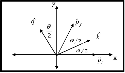
Figure 1: Scattering diagram in the xy-plane.

The above is, therefore, the specific form of the spin interaction in the first order S-matrix element of the elastic scattering of a single particle in any helicity-conserving vector potential regardless of its explicit form. Only applicability of the Born approximation is required. The above Hermitian SI operator $K$ (more precisely $\gamma_{5}K$) closes the $SU(2)$ algebra with other two operators in the spin space of the particle:

$$[\mathbf{\Sigma}.\mathbf{\hat{k}},\mathbf{\Sigma}.\mathbf{\hat{q}}] = 2i\Sigma_{3}$$

$$\left[\Sigma_{3},\mathbf{\Sigma}.\mathbf{\hat{k}}\right] = 2i\mathbf{\Sigma.\hat{q}}\$$ (13)

$$\left[\mathbf{\Sigma}.\mathbf{\hat{q}},\Sigma_{3}\right] = 2i\mathbf{\Sigma.\hat{k}},.$$

The following algebra can also be easily verified:

$$\left\{\mathbf{\Sigma}.\mathbf{\hat{k}},\mathbf{\Sigma}.\mathbf{\hat{q}}\right\}=\left\{\Sigma_{3},\mathbf{\Sigma}.\mathbf{\hat{k}}\right\}=\left\{\mathbf{\Sigma}.\mathbf{\hat{q}},\Sigma_{3}\right\}=0$$ (14)

Thus, the consequences:

$$(\mathbf{\Sigma.\hat{k}})^{2}=(\mathbf{\Sigma.\hat{q}})^{2}=(\Sigma_{3})^{2}=I.$$ (15)

The above results are suggestive of an interesting picture: Since the vectors $\mathbf{\hat{q}}$ and $\mathbf{\hat{k}}$ are ”intrinsic”, in that they are defined by the dynamics of the system, then it seems that a helicity-conserving system makes a natural choice of the representation of the generators of the $SU(2)$ in the spin space that goes along with its dynamics. The SI operator being one of these. Actually, the whole of the spin dynamics can be formulated in terms of the new ”intrinsic” axes and the corresponding spin operators ( see Fig.2). To see this, let us express the helicity operators in terms of the new generators $\mathbf{\Sigma.\hat{k}}$ and $\mathbf{\Sigma.\hat{q}}$ as

$$\mathbf{\Sigma.\hat{p_{i}}} = \cos\frac{\theta}{2}\mathbf{\Sigma.\hat{k}}-\sin\frac{\theta}{2}\mathbf{\Sigma.\hat{q}}$$

$$\mathbf{\Sigma.\hat{p_{f}}} = \cos\frac{\theta}{2}\mathbf{\Sigma.\hat{k}}+\sin\frac{\theta}{2}\mathbf{\Sigma.\hat{q}}$$ (16)

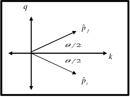
Figure 2: Scattering diagram in the $k-q$ plane.

Note the symmetry involved in these two expressions which is a reflection of the symmetry involved in Fig.2. With the above expressions in hand, it is easy to derive the following relations using the algebra , Eqs.(14);

$$K\mathbf{\Sigma.\hat{p_{i}}}K = \mathbf{\Sigma.\hat{p_{f}}}$$

$$K\mathbf{\Sigma.\hat{p_{f}}}K = \mathbf{\Sigma.\hat{p_{i}}},$$ (17)

from which we can easily rederive Eq.(10);

$$\mathbf{\Sigma.p_{f}}K\mathbf{\Sigma.p_{i}}=K.$$

Eq.(II) suggests that the incident and outgoing particles’ helicity operators are related through a reflection across the $\mathbf{\hat{k}}-$axis induced by the SI, $K$, and conservation of helicity in the transition can be expressed as the invariance of the components of the initial and final helicity states along the $\mathbf{\hat{k}}$-axis. Indeed, it is possible to express the eigenstates of $\mathbf{\Sigma.\hat{p_{i}}}$ and $\mathbf{\Sigma.\hat{p_{f}}}$ in terms of the eigenstates of $\mathbf{\Sigma.\hat{k}}$, viz.

$$|\hat{p}_{i},\pm\rangle = \cos\frac{\theta}{4}|\hat{k},\pm\rangle\mp\sin\frac{\theta}{4}|\hat{k},\mp\rangle$$

$$|\hat{p}_{f},\pm\rangle = \cos\frac{\theta}{4}|\hat{k},\pm\rangle\pm\sin\frac{\theta}{4}|\hat{k},\mp\rangle,$$ (18)

where use has been made of $\mathbf{\Sigma.\hat{q}}|\hat{k},\pm\rangle=|\hat{k},\mp\rangle$, which can be proven easily using the algebra,Eqs.(II) and (14). The following result then, follows immediately:

$$\langle\hat{k},\pm|\hat{p}_{i},\pm\rangle=\langle\hat{k},\pm|\hat{p}_{f},\pm\rangle=\cos\frac{\theta}{4}.$$ (19)

The component of the spin of the particle along the $\mathbf{\hat{k}}$-axis is indeed invariant in the transition.

III Aharonov-Bohm Vector Potential

In this section we consider as a concrete example of a vector potential the Aharonov-Bohm (AB) vector potential Y.Aharonov and D.Bohm (1959). We will show that the form of the SI, $K$, given by Eq.(12) follows for this potential. The (AB) potential conserves helicity in view of Eq.(1)as it does not generate an electric field. The conservation of helicity in the first order S-matrix was verified using explicit wave functions in F.Vera and I.Schmidt (1990). $\mathbf{A}(\mathbf{x})$ for this potential is planar and reads

$$\mathbf{A}=\frac{\Phi}{2\pi\rho}\hat{\epsilon}_{\varphi},$$ (20)

where $\rho=\sqrt{x^{2}+y^{2}}$, $\hat{\epsilon}_{\varphi}$ is the unit vector in the $\varphi$-direction, and $\Phi$ is the flux through the AB tube. Since the vector potential is planar , the dynamics is essentially planar by default in this case, and we can always take $\mathbf{p_{i}}=(p,0,0)\;,\;\mathbf{p_{f}}=(p\cos\theta,p\sin\theta,0)$, $\theta$ being the scattering angle. The first order S-matrix element,Eq.(5), upon plugging the above expression for $\mathbf{A}(\mathbf{x})$ then gives :

$$S^{(1)}_{fi}=-4\pi^{2}\Delta|N|^{2}\delta(E_{f}-E_{i})\frac{1}{q}<\mathbf{p_{f}};s_{f}|\frac{\alpha_{1}q_{2}-\alpha_{2}q_{1}}{q}|\mathbf{p_{i}};s_{i}>$$ (21)

Here, $\Delta=-e\Phi/2\pi$ (in perturbative calculations $0<\Delta<1$).Thus, comparing with Eq.(6), we identify $\frac{1}{q}$ with $|\mathbf{A}(\mathbf{q})|$ and $(\frac{\alpha_{1}q_{2}-\alpha_{2}q_{1}}{q})$ with $K$. It is easily checked that the above $K$ indeed has the specific form given by Eq.(12);

$$K=(\frac{\alpha_{1}q_{2}-\alpha_{2}q_{1}}{q})=\gamma_{5}\mathbf{\Sigma}.\mathbf{\hat{k}}$$

IV Conclusions

The dynamics of the elastic scattering of a Dirac particle in a vector potential ( magnetic field) in the first order Born approximation can always be reduced to a planar one by choosing a specific set of the coordinate axes. Thus, we have shown that the spin interaction (SI) ( the interaction that remains after integrating out the space degrees of freedom) in the first order scattering matrix for a general helicity-conserving vector potential assumes the specific form $K=\gamma_{5}\mathbf{\Sigma}.\hat{k}$, where $(\mathbf{\hat{k}}=\frac{\mathbf{p_{f}}+\mathbf{p_{i}}}{|\mathbf{p_{f}}+\mathbf{p_{i}}|}=(\cos\frac{\theta}{2},\sin\frac{\theta}{2},0)$ is a unit vector in the scattering plane that bisects the scattering angle $\theta$. The operator $\mathbf{\Sigma}.\hat{k}$ along with the two operators $\mathbf{\Sigma.\hat{q}}\,(\hat{q}=\frac{\mathbf{q}}{q},\,\mathbf{q}=\mathbf{p_{f}-p_{i}})$ and $\Sigma_{3}$ were shown to close the $SU(2)$. This means that $\mathbf{\Sigma.\hat{k}}$ and $\mathbf{\Sigma.\hat{q}}$ can be identified - in addition to $\Sigma_{3}$- as furnishing a representation of the generators of this group in the spin space of the particle. What is interesting with this representation is the fact that it is ” intrinsic’ in that the vectors $\mathbf{k}$ and $\mathbf{q}$ are defined by the dynamics of the system itself. It was shown that expressing the helicity operators of the initial and final states in terms of $\mathbf{\Sigma.\hat{k}}$ and $\mathbf{\Sigma.\hat{q}}$, the conservation of helicity in the transition can be viewed as the invariance of the $\mathbf{k}$-component of the helicity of the particle in the transition. As a concrete example , the AB potential was considered and the specific form of the SI was shown to emerge.

References

• J.J.Sakurai (1967) J.J.Sakurai, Advanced Quantum Mechanics (Addison-Wesley, Massachusettes, 1967).
• Y.Aharonov and D.Bohm (1959) Y.Aharonov and D.Bohm, Phys. Rev. 115, 485 (1959).
• A.Albeed and M.S.Shikakhwa (2004) A.Albeed and M.S.Shikakhwa (2004), eprint hep-th/0408093.
• F.Vera and I.Schmidt (1990) F.Vera and I.Schmidt, Phys.Rev. D 42, 3591 (1990).