Lab/UFR-HEP0502/GNPHE/0502/VACBT/0502
Hyperbolic Invariance in Type II Superstrings

Abstract

We first review aspects of Kac Moody indefinite algebras with particular focus on their hyperbolic subset. Then we present two field theoretical systems where these structures appear as symmetries. The first deals with complete classification of $\mathcal{N}=2$ supersymmetric CFT₄s and the second concerns the building of hyperbolic quiver gauge theories embedded in type IIB superstring compactification of Calabi-Yau threefolds. We show, amongst others, that $\mathcal{N}=2$ CFT₄s are classified by Vinberg theorem and hyperbolic structure is carried by the axion modulus.

Keywords: Classification of KM algebras, Indefinite KM sector and Hyperbolic subset, Quiver gauge theories embedded in type II superstrings.

1 Introduction

Kac Moody (KM) algebras $\mathbf{g}$ and their representations have been one of the basic tools in establishing strong results in quantum field and superstring theories. These particular bosonic algebras are generally divided into three basic sectors [1]: (1) Usual finite dimensional Lie algebras classified by Cartan; they play a crucial role in Yang-Mills gauge theories and in the understanding of the dynamics of interacting elementary particles. (2) Infinite dimensional affine KM algebras classified by Kac and Moody; they play a basic role in describing the physics of 2d scale invariant systems, in particular string world sheet dynamics [2] and a large class of statistical mechanics of 2d critical phenomena [3, 4]. (3) Indefinite KM algebras whose role in quantum physics is still unclear although they appear from time to time in physical literature as possible underlying symmetries in some specific models [5]-[13]. Besides of an apparent non unitary physical behaviour of hypothetical field theoretical models having indefinite algebras as symmetries, the little interest into these kind of systems might be also due to lack of complete mathematical results in this matter. To our understanding, the second reason is the most probable.

The aim of this study is to first make an excursion into indefinite sector of KM algebras. Then describe two examples where indefinite, in particular hyperbolic, KM algebras seem to appear as a physical invariance at least from theoretical point of view. These examples concerns:

(a) The full classification of $\mathcal{N}=2$ CFT₄ using geometric engineering method. As we will see, there are three classes of $\mathcal{N}=2$ CFT₄, one of them is classified by the indefinite subset of KM algebras.

(b) Embedding hyperbolic quiver gauge theories in type IIB superstring compactification on a specific class of K3 fibered Calabi-Yau threefolds (CY3). We show that the hyperbolic structure is captured by the axion field of ten dimensional type IIB string. Axion field carries therefore a trace on some hypothetical hidden indefinite KM (hyperbolic) symmetries in type IIB string.

The presentation of this paper is as follows: In section 1, I review briefly classifications of KM algebras. I give two theorems, one on the Vinberg classification of KM algebras and the other on the W. Li classification of their hyperbolic subset. In section 3, I expose aspects on geometric engineering method of 4d supersymmetric quiver gauge theories; in particular the engineering of fundamental matter. In section 4, I study the correspondences between the triplet: (i) roots $\alpha_{i}$ of KM algebras, (ii) 2-cycles $C_{i}$ of ADE geometries of CY3s and (iii) gauge coupling moduli $g_{i}$ in quiver gauge theories embedded in type II strings on CY3s. In section 5, I present two field theoretic systems where indefinite KM algebras appear as invariances. In section 6, I give a conclusion.

2 Classification theorems

To begin, let us recall some standard tools on Lie algebras, in particular roots, Cartan matrices and Dynkin diagrams. Given K, a symmetrisable square matrix with integers entries taken as follows,

$$K_{ii}=2;\qquad K_{ij}<0,\qquad K_{ij}=0\qquad\Rightarrow\qquad K_{ji}=0,$$ (2.1)

one generally associates a KM algebra $g=g\left(K\right)$ with the triplet $(\mathbf{\hbar},\Pi,\Pi^{\nu})$ realization defining respectively: (i) Commuting Cartan subalgebra generators $\left\{{H_{i}}\right\}$, (ii) the basis of simple roots $\left\{{\alpha}{{}_{i}}\right\}$ and ( iii) the basis of their coroots $\left\{\alpha_{i}^{v}\right\}$. Fo the case where K is symmetrisable, the situation to be considered here, KM algebras $g$ admit an invariant symmetric bi-linear form: $\left(,\right):g\times g\longrightarrow C$. In terms of this form, Cartan matrix K is realized as usual as

$$K_{ij}=<\alpha_{i}^{v},\alpha_{j}>=2\frac{(\alpha_{i},\alpha_{j})}{(\alpha_{i},\alpha_{i})}.$$ (2.2)

This relation reduces to $\alpha_{i}.\alpha_{j}$ for simply laced algebras for which there is one root length $\mathbf{(}\alpha,\alpha\mathbf{)}=2$. To fix ideas, I will focus my attention below this particular class.

2.1 Vinberg classification

Given above Cartan matrix $K$ and so the corresponding KM algebra $g\left(K\right)$, there is a powerful way to classify these matrices and algebras $g\left(K\right)$. This way, first introduced by Vinberg and then developed by KM, is a very constrained classification method. Its power follows from the fact that it is based on the existence of two positive vectors $\mathbf{u}$ and $\mathbf{v}$ (i.e several positive definite numbers $u_{i},v_{i}>0$) as required by following theorem.

Theorem:   A generalized indecomposable Cartan matrix $\mathbf{K}$ obeys one and only one of the following three statements:
(1) Finite type Lie algebras: g_finite ( $\det\mathbf{K}^{+}>0$ ):

This is the subset of usual finite dimensional Lie algebras g_finite; it is characterized by the existence of two real positive definite vectors $\mathbf{u=}\left(u_{1},...,u_{r}\right)$ and $\mathbf{v=}\left(v_{1},...,v_{r}\right)$ ($u_{i},v_{i}>0$) such that

$$\mathbf{K}_{ij}^{+}u_{j}=v_{j}>0.$$ (2.3)

The upper index on $\mathbf{K}^{+}$ is  introduced for convenience, its role will be understood in a moment.
(2) Affine type KM algebras, g_affine co-rank$\left(\mathbf{K}^{0}\right)=1$, $\det\mathbf{K}^{0}=0$,
For g_affine, there exist a unique, up to a multiplicative factor $\sigma$, positive integer definite vector $\mathbf{u}=\sigma\mathbf{d}$ ( $u_{i},d_{i}>0$) such that,

$$\mathbf{K}_{ij}^{0}u_{j}=\sigma\mathbf{K}_{ij}^{0}d_{j}=0.$$ (2.4)

This relation means that the affine Cartan matrix $K_{affine}$ has a vanishing eigenvalue. The $d_{i}$ integers are known as Dynkin weights.
(3) Indefinite type KM algebras, g_indefinite
For this class of KM algebras, and like for g_finite, there exist two real positive definite vectors $\mathbf{u=}\left(u_{1},...,u_{r}\right)$ and $\mathbf{v=}\left(v_{1},...,v_{r}\right)$ such that,

$$\mathbf{K}_{ij}^{-}u_{j}=-v_{i}<0.$$ (2.5)

As our present study relies on consequences of this basic theorem, let make four comments which will be used later. (a) Eqs(2.3-2.5) may be combined into a unique relation as follows

$$\mathbf{K}_{ij}^{q}u_{j}=qv_{i},$$ (2.6)

where $u_{i}$ and $v_{i}$ are as in Vinberg theorem and where $q=+1,0,-1$. Quantum number $q$ indexes then KM sectors. (b) For indefinite KM algebras, the sign of the determinant of $\mathbf{K}^{-}$ is indefinite; it may be either positive, zero or negative. This property is one of the features reflecting the difficulty in handling indefinite sector of KM algebras. (c) Indefinite feature of g_indefinite is also encoded by the negative sign of eq(2.6), which carries an indication on the fact bilinear from $\left(,\right)$ has an indefinite signature. Roots $\alpha$ of indefinite KM algebras are in general as follows,

$$\left(\alpha,\alpha\right)=2,1;\qquad\qquad\left(\alpha,\alpha\right)=2,1,0;\qquad\qquad\left(\alpha,\alpha\right)\leq 2;$$ (2.7)

(d) Unlike g_finite and g_affine, classification of indefinite sector is still an open question, except for some special cases where one disposes of partial results. The subset of hyperbolic algebras is one of these; it includes: (i) Standard hyperbolic algebras containing affine KM as a codimension one subalgebra and (ii) strictly hyperbolic ones containing only finite algebras as codimension one subalgebras. Examples of such specific subsets of KM algebras are given by the following $H\widehat{A}_{2}$ and $HB_{2}$ Dynkin diagrams,

Figure 1: Dynkin diagram of H$\widehat{\mathit{A}}_{2}$; the hyperbolic extension of affine $\widehat{\mathit{A}}_{2}$.

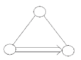
Figure 2: Dynkin diagram of HB₂; the hyperbolic extension of finite dimensional B₂.

Along with these two classes there are other subsets, in particular the so called extended hyperbolic algebras. Like for the strictly hyperbolic case, these extensions will not be examined in details in this contribution; so forget about them and focus on the special subset of hyperbolic algebras with codimension one affine KM subalgebras. For more information on the other issues, see [14] and refs therein.

2.2 W. Li classification

According to W. Li (WL) classification [15], there are $238$ hyperbolic Lie algebras containing the following special simply laced list,

$$\mathcal{H}_{1}^{4},\quad\mathcal{H}_{2}^{4},\quad\mathcal{H}_{3}^{4},\quad\mathcal{H}_{1}^{5},\quad\mathcal{H}_{8}^{5},\quad\mathcal{H}_{1}^{6},\quad\mathcal{H}_{5}^{6},\quad\mathcal{H}_{6}^{6},\quad\mathcal{H}_{1}^{7},$$

$$\mathcal{H}_{1}^{7},\quad\mathcal{H}_{1}^{8},\quad\mathcal{H}_{4}^{8},\quad\mathcal{H}_{5}^{8},\quad\mathcal{H}_{1}^{9},\quad\mathcal{H}_{4}^{9},\quad\mathcal{H}_{5}^{9},\quad\mathcal{H}_{1}^{10},\quad\mathcal{H}_{4}^{10},$$ (2.8)

where $\mathcal{H}$ refers to hyperbolic, the upper index stands for the rank of the hyperbolic algebra and the lower one for classification. Let us give details on some specific examples: The first example we give is $\mathcal{H}_{3}^{4}$ to be denoted also as $H\widehat{A}_{2}$. This is the simplest hyperbolic extension of affine KM algebra $\widehat{A}_{2}$ which appears as a particular subalgebra. $H\widehat{A}_{2}$ has four simple roots denoted as $a_{-1}$, $a_{0}$, $a_{1}$ and $a_{2}$ generating all other roots. The full set $\Delta_{hyp}\left(H\widehat{A}_{2}\right)$ of roots of $H\widehat{A}_{2}$ contains as a proper subset the roots of affine $\widehat{A}_{2}$ namely,

$$\pm\alpha_{1},\qquad\pm\alpha_{2},\qquad\pm\left(\alpha_{1}+\alpha_{2}\right),$$

$$n\delta,$$ (2.9)

$$n\delta\pm\alpha_{1},\qquad n\delta+\alpha_{2},\qquad n\delta\pm\left(\alpha_{1}+\alpha_{2}\right)$$

where the first line gives the usual roots of ordinary $A_{2}$ and where $\delta$ is the familiar imaginary root of affine KM algebras. In eqs(2.9) $n$ a non zero integer. The $H\widehat{A}_{2}$ algebra is a rank four KM algebra and has a $4\times 4$ Cartan matrix given by,

$$\mathbf{K}\left(HA_{2}\right)=\left(\begin{array}[]{cccc}2&-1&0&0\\ -1&2&-1&-1\\ 0&-1&2&-1\\ 0&-1&-1&2\end{array}\right).$$ (2.10)

Its Dynkin diagram, which is given by figure 1 has four nodes; it is composed of the two ordinary ones, the affine node and the hyperbolic one. The second example, we give concerns $H\widehat{D}_{4},$ the hyperbolic extension of affine $\widehat{D}_{4}$. Its Dynkin diagram has six nodes; four ordinary ones, one affine and one hyperbolic as shown on figure 3.

Figure 3: Hyperbolic extension of affine $\widehat{D}_{4}$. Node on left corresponds to hyperbolic extension.

Before proceeding, it is interesting to note that some algebras appearing in the WL classification appears as particular elements in the so called T_p,q,r algebras. Recall that Dynkin diagrams of $T_{p,q,r}$ involve 3 ordinary A_p, A_q and A_r Dynkin chains glued at a trivalent vertex. Exceptional algebras are the simplest examples; for instance $E_{10}$ indefinite KM algebra is just $E_{10}=T_{7,3,2}$; see also figure 4.

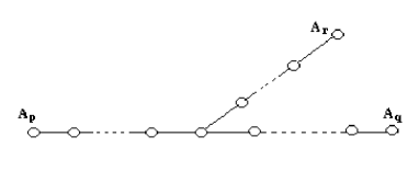
Figure 4: A typical vertex in trivalent algebras T_p,q,r  To the central node, it is attached three legs of A type.

The next note we give concerns useful aspects of T_p,q,r algebras; they will be used later on. On of these aspects is the value of the determinant Cartan matrix of T_p,q,r; which can be easily shown to be given by,

$$\det K\left(T_{p,q,r}\right)=pqrC_{3};\qquad C_{3}=\frac{1}{p}+\frac{1}{q}+\frac{1}{r}-1.$$ (2.11)

This a remarkable quantity for the study of classification of T_p,q,r algebras. Using this relation, one can recover results on the classification of finite and affine KM algebras. They are respectively associated with solving the necessary and sufficient conditions $C_{3}>1$ and $C_{3}=0$. Indefinite $T_{p,q,r}$ algebras corresponds to $C_{3}<1$. It should be noted also that eq(2.11) is in fact a particular example of a more general situation. Denoting $T_{p,q,r}$ as $T_{\left[3\right]}$ and following [16], the determinant $\det K\left(T_{\left[n\right]}\right)$ of n-dimensional vertex algebra $T_{\left[n\right]}$ reads as follows:

$$\det K\left(T_{\left[n\right]}\right)=C_{n}\mathop{\displaystyle\prod}\limits_{i=1}^{n}p_{i};\qquad C_{n}=\left(2-n\right)+\sum_{i=1}^{n}\frac{1}{p_{i}},$$ (2.12)

where the $p_{i}$s are non zero positive integers. As one see, $C_{n}$ is negative for large $n$.  For a more general formula regarding values of the determinant of Cartan matrices of indefinite KM algebra and the arithmetic that governs these computations can be found in [16]. Note finally that the conditions

$$C_{n}\geq n-2;\qquad n=2,3,...,$$ (2.13)

are very restrictive contrary to the constraint eq,

$$C_{n}<n-2;\qquad n=2,3,...,$$ (2.14)

which has infinitely many solutions and so infinitely many series of indefinite KM algebras.

3 Geometric engineering of $\mathcal{N}=2$ QFT₄s

Geometric engineering of $\mathcal{N}=2$ supersymmetric QFT₄s is a tricky method [17, 18, 19, 20, 21] to encode superfields contents of quiver gauge theories embedded in type IIA string compactification on Calabi-Yau threefolds with ADE geometries. In this picture, gauge and adjoint matter are associated with nodes of ADE Dynkin diagrams and bi-fundamental matter with links between nodes.

Result:  In $\mathcal{N}=1$ supersymmetric language, Gauge multiplets, adjoint matter and bi-fundamental one are naturally encoded by Dynkin diagrams of finite and affine KM algebras. But what about fundamental matter transforming in the fundamental representation of $G_{gauge}\times G_{flavor}$ symmetry ?

3.1 Adding fundamental matter

Adding fundamental matter in $\mathcal{N}=2$ QFT₄s requires more than Dynkin diagrams; it needs the so called trivalent geometry. This is the other reason behind our previous interest into $T_{p,q,r}$ KM algebras, the first one concerned examples of indefinite KM algebras. $T_{p,q,r}$ Dynkin diagrams have an extra third chain which may be used to encode fundamental matter. However this is not a soft operation; there is a price one should pay for engineering fundamental matter in term of trivalent geometry. The reason is that Calabi-Yau condition fulfilled by ADE geometries is no longer present for trivalent geometries. Restoring Calabi-Yau condition requires promoting $T_{p,q,r}$ to a tetravalent geometry which we will denote as $T_{p,q,r,-s}$, see also figure 5. As this generalized geometry is behind engineering of fundamental matter, let us say few more words on it.

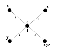
Figure 5: This is a typical vertex for engineering  fundamental matter in supersymmetric $\mathcal{N}=2$ QFT₄s. It may be noted as $T_{2,2,2,-2}$, the negative integer refers to promotion of original trivalent geometry $T_{2,2,2}$ into a CY one.

Generalized geometry $T_{p,q,r,-s}$ involves the following typical dimension three vertices $V_{i}$,

$$V_{0}=\left(0,0,0\right);\quad V_{1}=\left(1,0,0\right);\quad V_{2}=\left(0,1,0\right);\quad V_{3}=\left(0,0,1\right);\quad V_{4}=\left(1,1,1\right),$$ (3.1)

satisfying the following toric geometry relation

$$\sum_{i=0}^{4}q_{i}V_{i}=-2V_{0}+V_{1}+V_{2}+V_{3}-V_{4}=0$$ (3.2)

The vector charge $\left(q_{i}\right)=\left(-2,1,1,1,-1\right)$ is known as the Mori vector and the sum of its $q_{i}$ components is zero as required by the CY condition;

$$\sum_{i}q_{i}=0.$$ (3.3)

Before going ahead it is interesting to note that extension, of trivalent geometry to Calabi Yau one, has an interpretation on the KM algebra side. Let us illustrate this on analyzing corresponding ”Cartan” matrices of trivalent KM algebra and its CY extension. The promotion feature of trivalent geometry $T_{2,2,2}$ into the CY $T_{2,2,2,-2}$ one is in fact a very special extension. To $T_{2,2,2}$ vertex corresponds, on Lie algebraic side, the following $4\times 4$ Cartan matrix

$$K\left(T_{2,2,2}\right)=\left(\begin{array}[]{cccc}2&0&-1&0\\ 0&2&-1&0\\ -1&-1&2&-1\\ 0&0&-1&2\end{array}\right)$$ (3.4)

with $\det\left(T_{2,2,2}\right)=$ $4$; while for the CY extension, we have the following $5\times 5$ matrix

$$K\left(T_{2,2,2,-2}\right)=\left(\begin{array}[]{ccccc}2&0&-1&0&0\\ 0&2&-1&0&0\\ -1&-1&2&-1&1\\ 0&0&-1&2&0\\ 0&0&1&0&2\end{array}\right).$$ (3.5)

Strictly speaking, $K\left(T_{2,2,2,-2}\right)$ is no longer a Cartan matrix type since not all $K_{ij}$s, $i\neq j$, are negative integers as required by eq(2.1). Following [16], its determinant $\det\left(T_{2,2,2,-2}\right)$ is given by

$$\det\left(T_{2,2,2,-2}\right)=\det A_{1}\det T_{2,2,2}-\left(\det A_{1}\right)^{3},$$ (3.6)

which vanishes identically since $2\times 4-2^{3}=0$. Note also that $T_{2,2,2,-2}$ should be distinguished from $T_{2,2,2,2}$ which is a KM algebra with a $5\times 5$ Cartan matrix given by,

$$K\left(T_{2,2,2,2}\right)=\left(\begin{array}[]{ccccc}2&0&-1&0&0\\ 0&2&-1&0&0\\ -1&-1&2&-1&-1\\ 0&0&-1&2&0\\ 0&0&-1&0&2\end{array}\right)$$ (3.7)

and whose determinant vanishes as well, $\det\left(T_{2,2,2,2}\right)=0$. The difference between eqs(3.7) and (3.5) is that while in the present case Dynkin vector is positive definite as shown below,

$$\mathbf{d}=\left(1,1,2,1,1\right),$$ (3.8)

its analog for $T_{2,2,2,-2}$ is no longer positive definite as is it given by $\widetilde{\mathbf{d}}=\left(1,1,2,1,-1\right)$. It follows then $T_{2,2,2,-2}$ does not fulfill Vinberg theorem requirements and so sits beyond of KM classification.

3.2 Mirror geometry

In type IIB strings on mirror CY3, the $\left(V_{0},V_{1},V_{2},V_{3},V_{4}\right)$ vertices are represented by complex variables $\left(u_{0},u_{1},u_{2},u_{3},u_{4}\right)$ constrained as

$$\prod_{i}u_{i}^{q_{i}}=1$$ (3.9)

and solved by $\left(1,x,y,z,xyz\right)$; see figure 5. In terms of these variables, the algebraic eq describing mirror geometry, associated to eq(3.2), is given by the following complex surface,

$$P\left(X^{\ast}\right)=\mathrm{e}+\mathrm{a}x+\mathrm{b}y+\left(\mathrm{c}-\mathrm{d}xy\right)z,$$ (3.10)

where $\mathrm{a,b,c,d}$ and $\mathrm{e}$ are complex moduli. Note that upon eliminating the $z$ variable, the above (trivalent) algebraic geometry eq reduces exactly to the standard bivalent vertex of $A_{1}$ geometry,

$$P\left(X^{\ast}\right)=\mathrm{a}x+\mathrm{e}+\frac{\mathrm{bc}}{\mathrm{d}}\frac{1}{x}.$$ (3.11)

The monomials $y_{0}=x$, $y_{1}=1$ and $y_{2}=\frac{1}{x}$ satisfy the well known $su\left(2\right)$ relation namely $y_{0}y_{2}=y_{1}^{2}$. To get algebraic geometry eq of the CY3, one promotes the non zero moduli $\mathrm{a,b,c,d}$ and $\mathrm{e}$ to holomorphic polynomials on $\mathbb{CP}^{1}$ as follows:

$$\mathrm{e}\left(w\right) = \sum_{i=0}^{n_{r}}\mathrm{e}_{i}w^{i};\qquad\mathrm{a}\left(w\right)=\sum_{i=0}^{n_{r-1}}\mathrm{a}_{i}w^{i};\qquad\mathrm{b}\left(w\right)=\sum_{i=0}^{n_{r+1}}b_{i}w^{i},$$

$$\mathrm{c}\left(w\right) = \sum_{i=0}^{m_{r}}c_{i}w^{i};\qquad\mathrm{d}\left(w\right)=\sum_{i=0}^{m_{r}^{\prime}}d_{i}w^{i};\qquad\mathrm{e}_{0},\mathrm{a}_{0},\mathrm{b}_{0},\mathrm{c}_{0},\mathrm{d}_{0}\neq 0.$$ (3.12)

These analytic polynomials encode the fibrations of,

$$SU\left(1+n_{r-1}\right)\times SU\left(1+n_{r}\right)\times SU\left(1+n_{r+1}\right),$$ (3.13)

gauge invariance of the underlying $\mathcal{N}=2$ QFT₄ and its,

$$SU\left(1+m_{r}\right)\times SU\left(1+m_{r}^{\prime}\right),$$ (3.14)

flavor symmetry. These groups are engineered over the five nodes of the extended trivalent vertex (CY 4-vertex). For instance $SU\left(1+n_{r-1}\right)$ gauge symmetry is fibered over $V_{0}$ and $SU\left(1+m_{r}\right)$ and $SU\left(1+m_{r}^{\prime}\right)$ flavor invariance are fibered over the nodes $V_{3}$ and $V_{4}$ respectively; see figure 6.for illustration. Note in passing that $m_{r}^{\prime}$ refers to engineering of fundamental matter on the extra node we have added to recover CY condition.

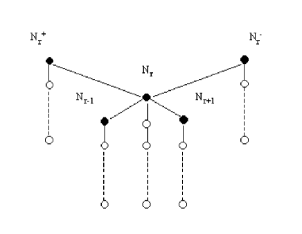
Figure 6: This is a typical vertex of geometric engineering of $\mathcal{N}\mathit{=2}$ supersymmetric QFT₄. $SU\left(1+l_{i}\right)$ gauge and flavor symmetries are fibered over the five black nodes. Flavor symmetries require large base volume.

4 Roots and 2-cycles in $\mathcal{N}=2$ QFT₄s

Here we consider the WL hyperbolic extension of affine ADE quiver gauge theories. Since these hyperbolic algebras are simplest extensions of affine ADE ones, one can easily make an idea on this larger structure just by trying to extend known results.

4.1 Simple roots in hyperbolic model

We can write down several relations for hyperbolic ADE Lie algebras just by using intuition and similarity arguments. Starting from a rank r affine simply laced KM algebra with the usual simple roots $\alpha_{i},$ $i=0,1,...,r,$ and

$$\alpha_{0}=\delta-\sum_{i=1}^{r}d_{i}\alpha_{i}$$ (4.1)

where $\delta$ stands for the usual imaginary root; $\delta^{2}=0$, we can immediately write down a realization of simple roots of the hyperbolic extension. The rule is as follows: (a) Fix an affine ADE Cartan matrix $K_{ij}^{0}=\alpha_{i}.\alpha_{j}$ and so a Dynkin diagram $\mathcal{D}^{0}$. We have for the case of affine A_r the following realization,

$$\alpha_{i}=e_{i}-e_{i+1};\qquad\alpha_{0}=\delta-\psi,$$ (4.2)

where $\left\{e_{i}\right\}$ is a basis of orthonormal vectors. (b) Add an extra simple root $\alpha_{-1}$ to the game with the constraint eqs,

$$\alpha_{-1}.\alpha_{-1}=2;\qquad\alpha_{-1}\alpha_{0}=-1;\qquad\alpha_{-1}\alpha_{i}=0.$$ (4.3)

(c) Because of the Lorentzian nature of the root lattice of hyperbolic ADE algebras, this extra simple root is realized as,

$$\alpha_{-1}=\gamma-\delta;\qquad\gamma^{2}-2\gamma.\delta+\delta^{2}=2,$$ (4.4)

with $\gamma$ being a second basic imaginary root exhibiting the properties:

$${\gamma}^{2} = {\delta}^{2}=0;\qquad{\gamma}{\delta}=-1,$$

$${\gamma.}\alpha_{0} = 1;\qquad{\gamma.}\alpha_{i}=0,\ i>0.$$ (4.5)

Before proceeding, let us give some useful results: (i) Hyperbolic ADE Lie algebras have two basic (light like) imaginary roots $\gamma$ and $\delta$  and so two special affine subalgebras. (ii) $\gamma$ and $\delta$ play a completely symmetric role. This symmetry is just a specific Weyl transformation of root system in hyperbolic algebra. (iii) The symmetry between $\gamma$ and $\delta$ may be used to extract part of information on hyperbolic structure that are not captured by affine KM subsymmetry.

4.2 2-Cycles in Calabi-Yau threefolds

Root system $\left\{\alpha\in\Delta\right\}$ of KM algebras have a remarkable interpretation in algebraic geometry and in quiver gauge theories embedded in type II string compactification on CY3 with ordinary and affine ADE geometries. Following [17], see also [19]-[21], there is a one to one correspondence between the following pairs: ADE algebra $\longleftrightarrow$ ADE geometry and ADE geometry $\longleftrightarrow$ $\mathcal{N}=2$ quiver gauge theories. More precisely, to each root $\alpha$, say the $su\left(n\right)$ simple root $\alpha_{i}=e_{i}-e_{i+1}$, corresponds a two cycle $C$ (a basis 2-cycles $C_{i}$) of the ADE geometry of CY3. We have the following 2-cycles intersection formula,

$$C_{i}\cdot C_{i}=-K_{ij},$$ (4.6)

where $K_{ij}$ is exactly the Cartan matrix of ADE algebra. The holomorphic volumes $v_{i}=t_{i}-t_{i+i}$ the 2-cycle $C_{i}$ basis are interpreted in quiver gauge theories in terms of gauge coupling moduli as shown below,

$$g_{i}^{-2}\sim\left|t_{i}-t_{i+i}\right|.$$ (4.7)

Here $t_{i}$ are complex moduli. In general, we have the following correspondences: (1) ADE algebra $\longleftrightarrow$ ADE geometry,

Simple roots ​αi⟷2-Cycles ​Ci=ℙi1Imaginary δ⟷2-Torus 𝕋2Weyl transformations ω⟷Picard group,fragments Simple roots αifragments⟷fragments2-Cycles Ci=ℙi1fragmentsImaginary δfragments⟷fragments2-Torus T2fragmentsWeyl transformations ωfragments⟷Picard group\begin{tabular}[]{|l|l|l|}\hline\cr Algebra&$\qquad\longleftrightarrow\qquad$&Geometry\\ \hline\cr{Simple roots}$\text{\ }\alpha_{i}$&$\qquad\longleftrightarrow\qquad$&$2${-Cycles}$\text{ }C_{i}=\mathbb{P}_{i}^{1}$\\ \hline\cr{Imaginary} $\delta$&$\qquad\longleftrightarrow\qquad$&$2${-Torus} $\mathbb{T}^{2}$\\ \hline\cr$\text{{Weyl transformations} }\omega$&$\qquad\longleftrightarrow\qquad$&{Picard group}\\ \hline\cr\end{tabular},

Algebra⟷GeometryAlgebra⟷Geometry (4.8)

where $\omega$ belongs to $W_{affine}$; the affine Weyl group generated by reflections $r_{\alpha}$ and translations $t_{\alpha}$. These transformations, which generate two proper subgroups of $W_{affine}$, are defined as,

$$\omega_{\alpha}\left(\beta\right) = \beta-2\frac{\left(\alpha,\beta\right)}{\alpha^{2}}\alpha,,$$

$$t_{\alpha}^{\delta}\left(\beta\right) = \beta+(\delta,\beta)\alpha-\left(\alpha,\beta\right)\delta-\frac{\alpha^{2}}{2}\left(\delta,\beta\right)\delta,$$ (4.9)

and simplify for simply laced affine KM algebras. For $\beta\in\Delta_{finite}$, the translation $t_{\alpha}^{\delta}\left(\beta\right)$ takes a simple form namely $\beta-\left(\alpha,\beta\right)\delta$. (2) ADE geometry $\longleftrightarrow$ Quiver QFT₄

Geometry $$\qquad\longleftrightarrow\qquad$$ Quiver gauge theory

;

Weyl symmetry Seiberg like duality

(4.10)

where $\phi$ is dilaton. Following [14, 23], the above correspondence, which involves the triplet composed by roots of affine KM algebra, 2-cycles of ADE geometry and gauge moduli in $4d$ $\mathcal{N}=2$ quiver gauge theories, may be extended naturally to hyperbolic KM algebras and likely to the more general indefinite ones. Similarly to above affine model, one also has a correspondence between hyperbolic root system, 2-cycles and gauge moduli in hyperbolic gauge theories. We have the following results:

4.2.1 Hyperbolic algebra $\longleftrightarrow$ hyperbolic geometry

To start recall that simple root basis of hyperbolic extension of affine ADE algebras involves, in addition to $\left\{\alpha_{0},\alpha_{i}\right\}$, an extra simple root $\alpha_{-1}$ whose Lie algebra features are given by eqs(4.4-4.5). The simple root system $\left\{\alpha_{-1},\alpha_{0},\alpha_{i}\right\}$ involves, amongst others, the two imaginary roots $\gamma$ and $\delta$,

$$\delta=\sum_{i=0}^{r}d_{i}\alpha_{i};\qquad\gamma=\sum_{i=-1}^{r}d_{i}\alpha_{i},$$ (4.11)

where $d_{i}$, $0\leq i\leq r$ are the usual Dynkin weights and where $d_{-1}$, which is equal to one, is their hyperbolic analog. Extending results on type II string interpretation of affine models to the hyperbolic ADE case, we see that geometrically speaking, $\gamma$ and $\delta$ generate two heterotic torii $T_{\pm}^{2}$,

$$T_{+}^{2}=\sum_{i=0}^{r}d_{i}S_{i}^{2};\qquad T_{-}^{2}=\sum_{i=-1}^{r}d_{i}S_{i}^{2},$$ (4.12)

where, roughly speaking, the $S_{i}^{2}$s are the usual real two spheres of type II strings on CY3s with deformed ADE singularities. $S_{-1}^{2}$ is the 2-sphere associated with the root $\alpha_{-1}$.

Hyperbolic algebra $$\qquad\longleftrightarrow$$ hyperbolic geometry

Simple root 2-sphere

Imaginary root 2-torus

Imaginary root 2-torus

Intersection  

(4.13)

Note that $T_{+}^{2}$ and $T_{-}^{2}$ may be thought of as holomorphic $T_{z}^{2}$ and anti-holomorphic $T_{\overline{z}}^{2}$ two cycles in Kahler threefolds. This observation constitutes a key point in our quest for searching indefinite symmetries in hyperbolic ADE quiver gauge models.

4.2.2 Hyperbolic geometry $\longleftrightarrow$ hyperbolic gauge model

Extending results on type IIB superstring interpretation of 4d $\mathcal{N}=2$ affine quiver gauge theories, it is not difficult to see that the following correspondence holds,

hyperbolic geometry $$\qquad\longleftrightarrow\qquad$$ hyperbolic QFT₄

Weyl symmetry generalized Seiberg like duality

(4.14)

Like for $Vol\left(C_{0}\right)$, this correspondence allows us to interpret $Vol\left(C_{-1}\right)$ in terms of type IIB string moduli space, except now that we should have a non zero action $\chi$. Note that, upon performing a Wick rotation of the RR axion moduli ($\chi\longrightarrow i\chi$), the inverse string coupling $g_{+}^{-1}$ becomes $g_{\tau}^{-1}=exp(-\phi)-i\chi$ which should be compared with the complex moduli $i\tau_{IIB}$ of the holomorphic two torus used in F-theory compactification on elliptic K3 [24].

5 Hyperbolic invariance: Two examples

In this section, we present two field theoretical models where hyperbolic invariance appears as a symmetry. The first example deals with the complete classification of $\mathcal{N}=2$ CFT₄ in four dimensions. The second example concerns $\mathcal{N}=2$ hyperbolic quiver gauge theories embedded in type IIB superstrings on CY3s; but with non zero axion.

5.1 Example I: Classification of $N=2$ CFT₄s

Four dimensional $N=2$ supersymmetric CFTs constitute an important class of QFT₄s embedded in type II superstring compactifications on elliptic fibered CY threefolds with $ADE$ geometries preserving eight supersymmetries. These special field theoretic models give exact solutions for the moduli space of the Coulomb branch of $\mathcal{N}=2$ QFT₄s and admit a very nice geometric engineering in terms of quiver diagrams. Common $\mathcal{N}=2$ CFT₄s were first believed to be classified into two categories according to the type of singularities; but as we will see, there are in fact three categories classified by Vinberg theorem.

(1) Ordinary super CFT₄s:$\qquad\mathcal{N}=2$ supersymmetric CFT₄ based on finite $ADE$ singularities with quiver gauge group,

$$G=\prod_{i}SU\left(n_{i}\right)\times G_{flavor}$$ (5.1)

and matter in both fundamental $\mathbf{n}_{i}$ and bi-fundamental $\left(\mathbf{n}_{i}\mathbf{,}\overline{\mathbf{n}}_{j}\right)$ representations of $G$.

(2) Affine super CFT₄s:$\qquad\mathcal{N}=2$ CFT₄ with quiver gauge group

$$G=\prod_{i}SU\left(d_{i}n\right),$$ (5.2)

and bi-fundamental matter only. This second category of scale invariant field models are classified by affine $ADE$ algebras. The positive integers $d_{i}$ appearing in $G$ are the usual Dynkin weights considered earlier; they form a special positive definite integer vector $\mathbf{d}=\left(d_{i}\right)$ satisfying $\mathbf{K}_{ij}^{0}d_{j}=0$ and so

$$\mathbf{K}_{ij}^{0}n_{j}=0.$$ (5.3)

Here $n_{j}=nd_{j}$ and $\mathbf{K}^{0}$ is the affine Cartan matrix. Before describing the third class, let us comment a little bit the emergence of eq(5.3) in the CFT game. Though not surprising, the appearance of this remarkable eq in the geometric engineering of $\mathcal{N}=2$ CFT₄s is very exciting. First because $4d$ conformal invariance requiring the vanishing of the total holomorphic beta function $b,$ which requires in turn the vanishing of the beta function factors $b_{i}$,

$$b_{i}=\frac{1}{12}\left(44n_{i}-2\sum_{j}\left[4a_{ij}^{4}+a_{ij}^{6}\right]n_{j}\right),\qquad 3a_{ij}^{4}=3\overline{a}_{ij}^{4}=2a_{ij}^{6},$$ (5.4)

is now translated into a condition on allowed KM algebras eq(5.3). In above relation $a_{ij}^{4}$ is the number of fundamental fermions and $a_{ij}^{6}$ the number of adjoint scalars. Second, even for $\mathcal{N}=2$ CFT₄ based on finite $ADE$ with $m_{i}\mathbf{n}_{i}$ fundamental matters, the condition for scale invariance may be also formulated in terms of the corresponding Cartan matrix $\mathbf{K}^{+}$ as,

$$\mathbf{K}_{ij}^{+}n_{j}=m_{i}.$$ (5.5)

Note that identities (5.3,5.5) can be rigorously derived by starting from mirror geometry of type IIA string on Calabi-Yau threefolds and taking the field theory limit in the weak gauge couplings $g_{r}$ regime associated with large volume of the CY3 base ( $V_{r}=1/\varepsilon$ with $\varepsilon\rightarrow 0$ ). In this limit and using eqs(3.10-3.12) and figure 6, one shows that complex deformations $a_{r,l}$, $b_{r,l}$, $c_{r,l}$, $d_{r,l}$ and $e_{r,l}$ of the mirror geometry scale as,

$$a_{r,l} = \varepsilon^{l-n_{r-1}},\qquad b_{r,l}=\varepsilon^{l-n_{r+1}},\qquad c_{r,l}=\varepsilon^{l-m_{r}},$$

$$d_{r,l} = \varepsilon^{l-m_{r}^{\prime}},\qquad e_{r,l}=\varepsilon^{l-n_{r}},$$ (5.6)

where $m_{r}^{\prime}$ is taken non zero for later consideration. One shows moreover that the universal coupling parameters $Z\left(g_{r}\right)$ given by,

$$Z\left(g_{r}\right)=\frac{a_{r,0}b_{r,0}c_{r,0}}{e_{r,0}^{2}d_{r,0}},$$ (5.7)

behave as $\varepsilon^{-b_{r}}$ with $b_{r}$s, the beta function components of the $r$-th $U\left(n_{r}\right)$ gauge subgroup factor of $G$; given by,

$$b_{r}=2n_{r}-n_{r-1}-n_{r+1}-\left(m_{r}-m_{r}^{\prime}\right).$$ (5.8)

In the limit $\varepsilon\rightarrow 0$, finiteness of universal couplings $Z^{\left(g_{r}\right)}$ requires $b_{r}\leq 0$; i.e the field theory limit should be asymptotically free. Scale invariance of the $\mathcal{N}=2$ CFT₄s requires however $b_{r}=0$  for all $r$ indices. Upon setting

$$u_{i}=n_{i};\qquad v_{i}=\left|m_{i}-m_{i}^{\prime}\right|,$$ (5.9)

it is not difficult to see that eq(5.8) coincide exactly with eqs(5.3,5.5). The vanishing condition of $b_{r}$s is then translated into a condition on the intersection matrix ( Cartan matrix) $K_{ij}^{\left(q\right)}$ of $ADE$ singularities one is considering; i.e finite, affine or indefinite. As a result, one sees that, along with ordinary and affine supersymmetric CFT₄s, there is moreover an extra remarkable indefinite sector. In what follows, we will give comments on indefinite CFTs; for more details and technicalities see [17, 14, 22].

(3) Indefinite $\mathcal{N}=2$ CFT₄s:       To start, note that appearance of eqs(5.3,5.5) can be viewed as just the two leading relations of a more general result associated with the triplet,

$$\mathbf{K}_{ij}^{q}n_{j}=qv_{i};\qquad q=+1,0,-1.$$ (5.10)

From this view, one already suspects that $\mathcal{N}=2$ CFT₄s should be classified by Vinberg formula eq(2.6). At a first sight, this relation tells us, amongst others, that: (i) there are three main classes of $\mathcal{N}=2$ CFT₄s, (ii) the extra indefinite $\mathcal{N}=2$ CFT₄ sector is given by,

$$\mathbf{K}_{ij}^{-}n_{j}=-v_{i}.$$ (5.11)

Following [14, 22, 23] and using above analysis eqs(5.6-5.9), one shows that eq(5.10) do follow indeed from type II string on Calabi-Yau threefolds with geometries having a 2-cycle basis $\left\{C_{i}\right\}$ satisfying,

$$C_{i}\cdot C_{i}=\mathbf{K}_{ij}^{q};\qquad q=+1,0,-1.$$ (5.12)

The derivation of eq(5.10) is then proved; it relies on using trivalent geometry (figure 6) and proceeds as in eq(3.10-3.12) by considering the general representation of fundamental engineering fundamental matter. Let re-comment briefly the main steps by using different, but equivalent, sentences: (i) Use geometric engineering of $\mathcal{N}=2$ QFT₄s described in section 3. (ii) Fundamental matter require extension of trivalent vertices with the five entry Mori vectors,

$$q_{\mathrm{\tau}}=\left(1,-2,1;1,-1\right).$$ (5.13)

The first three ones namely $\left(1,-2,1\right)$ are common entries since they are involved in the geometric engineering of gauge fields and bi-fundamental matter. They lead to $\mathbf{K}_{ij}^{0}n_{j}=0$. The fourth entry is used in the engineering of fundamental matter of CFT₄s based on finite $ADE$ and lead to $\mathbf{K}_{ij}^{+}n_{j}=m_{i}$. The fifth entry has been treated for sometimes as a spectator only needed to ensure the CY condition $\sum_{\tau=1}^{5}q_{\mathrm{\tau}}=0$. Handling this vertex on equal footing as the four previous others; i.e $m\prime_{i}\neq 0$ in eq(5.6), gives surprisingly the missing third sector of eqs(5.10).

Result:  $\mathcal{N}=2$ CFT₄s, embedded in type II string compactification on Calabi-Yau threefolds with generalized ADE geometries satisfying eqs(5.12), are classified by Vinberg classification theorem of KM algebras.

5.2 Example II: Axion as a hyperbolic moduli

To begin recall that 4d supersymmetric ADE quiver gauge theories are QFT₄ limits of type II strings on CY threefolds with ADE geometries and are remarkably engineered on ADE Dynkin diagrams. Nodes of the Dynkin graphs encode gauge and adjoint matter multiplets. Links between the nodes engineer bi-fundamental matter involved in supersymmetric $\prod_{i}U\left(N_{i}\right)$ quiver gauge theory. Recall also that roots $\alpha$ of KM algebras,

$$\alpha=\pm\sum_{i}k_{i}\alpha_{i},\qquad k_{i}\in\mathbb{Z}_{+},$$ (5.14)

which are generated by the $\alpha_{i}$ simple ones, are generally realized in $\mathbb{R}^{n}=\sum\mathbb{R}e_{i}$ in terms of specific linear combinations of the $\left\{e_{i}\right\}$ basis, $e_{i}e_{j}=\delta_{ij}$. For the case of $su\left(n\right)$ simple roots for instance, we have

$$\alpha_{i}=e_{i}-e_{i+1},\qquad i=1,....$$ (5.15)

Together with this eq, there are also relations such that $\alpha_{1}+...+\alpha_{n}=e_{1}-e_{n+1}$ which are useful in the study of quiver gauge theories. With these results in mind; one can go ahead to study supersymmetric QFT₄s embedded in type II strings on CY3 with ADE geometries and their hyperbolic extension.  To that purpose, recall that roots have algebraic geometry analogs in CY3 with generalized ADE geometries. Some of the results regarding this correspondence were already shown on eqs(4.8-4.13). In what follows, we complete the picture of subsection 5.1 by giving details and comments.

One of the relevant objects for our study concerns the correspondence between roots of simply laced KM algebra and 2-cycles of the associated geometry. Of particular interest are simple roots $\alpha_{i}$ which are in one to one correspondence with the holomorphic ”volumes” $\zeta_{i},$

$$\zeta_{i}=\int_{\mathbb{P}_{i}^{1}}\Omega^{\left(2,0\right)}.$$ (5.16)

In this eq, $\Omega^{\left(2,0\right)}$ is the usual holomorphic two form on the complex dimension one projective space $\mathbb{P}^{1}$. So the $\zeta_{i}$s are the volumes of the homological two-cycles $\mathbb{P}_{i}^{1}\sim S_{i}^{2}$ involved in the deformation of ADE singularities. Let us make two comments regarding these complex holomorphic volumes $\zeta_{i}$. First, note that their explicit values are given by,

$$\zeta_{i}=t_{i}-t_{i+1},\qquad i=1,....,$$ (5.17)

where $t_{i}$s are complex moduli. These values should be compared with eq(5.15) and allow to write down holomorphic volumes of any 2-cycles of the ADE geometry by just using the analogy of roots. Second the $\zeta_{i}$s, which describe deformations of local ADE geometry, have a nice interpretation in $4d$ $\mathcal{N}=2$ supersymmetric quiver $\Pi_{i=1}^{r}U\left(N_{i}\right)$ gauge theories with adjoint matter superfields $\left\{\Phi_{i}\quad i=1,...,r\right\}$. They appear as FI like coupling constants generating the following $4d$ $\mathcal{N}=1$ linear chiral superspace potential deformation $\mathrm{\delta W}$,

$$\mathrm{\delta W}=\sum_{i=1}^{r}\zeta_{i}\int d^{4}xd^{2}\theta Tr\left(\Phi_{i}\right)\text{.}$$ (5.18)

This special superpotential deformation preserves $\mathcal{N}=2$ supersymmetry and its non linear $\mathcal{N}=1$ extension $\mathrm{\delta W}\sim\Phi^{n+1}$ is at the basis of the field theoretic representation of the geometric transition $O\left(-1\right)\times O\left(-1\right)\times\mathbb{CP}^{1}\rightarrow T^{\ast}S^{3}$ of the conifold. Eq(5.18) is also behind the field theoretic analysis of large $N$ field dualities and in the derivation of exact results in $\mathcal{N}=1$ supersymmetric gauge theories.

The other relevant object we want to give here concerns Weyl group rotating roots of hyperbolic KM algebra and duality symmetry in hyperbolic quiver gauge theories. For affine ADE KM algebras, it is now well established that Weyl group $W_{ADE}$ is associated with Seiberg like dualities and its translation subgroup is behind the RG cascades of affine models. At low energies below string scale where the dynamics of matter and gauge fields is governed by supersymmetric Yang Mills model, one disposes of sets of dual ADE quiver gauge theories with a remarkable subclass whose duality symmetries act on previous $\upsilon_{i}$ as

$$\upsilon_{i}\rightarrow\upsilon_{i}^{\prime}=A_{ij}\upsilon_{j},$$ (5.19)

These duality symmetries were shown to be isomorphic to the usual Weyl group transformations of ADE root system [26]. By help of correspondence (5.19), the $A_{ij}$ matrix in above relation is isomorphic to the bi-linear product $\delta_{ij}-\alpha_{i}\alpha_{j}$ that appears in Weyl reflections,

$$\alpha_{i}^{\prime}=\alpha_{i}-2\frac{\alpha_{i}\alpha_{j}}{\alpha_{j}^{2}}\alpha_{j}.$$ (5.20)

In addition to the two above links, there are other basic links between $4d$ super quiver QFT₄s and ADE algebra. For instance ADE root systems and their Weyl symmetries are also used in brane realization of the quiver gauge theories living in the world volume of parallel $N_{0}$ D3 branes and $N$ D5 ones partially wrapping CP${}_{i}^{1}$ two-cycles of CY3 folds with a local ADE geometry. There, $N_{0}$ D3 are roughly speaking associated with the affine simple root $\alpha_{0}$ of affine KM ADE root system and wrapped $N$ D5s with remaining $\alpha_{i}$ simple ones. In this representation, field theoretic scenarios such as higgsings correspond just to special properties of the root system. Other basic relations between roots and their Weyl automorphisms on one hand; and relevant QFT₄ moduli on the other hand can be also written down. Supersymmetric Yang-Mills gauge couplings g${}_{i}^{SYM}$ of the quiver gauge subgroup factors $U\left(N_{i}\right)$ and corresponding beta functions $b_{i}$ including supersymmetric affine ADE conformal field models,

$$\frac{1}{g_{s}}=\sum_{i=0}^{r}d_{i}g_{i}^{-2};\qquad b_{D}=\sum_{i=0}^{r}d_{i}b_{i},$$ (5.21)

obey a similar law as holomorphic volumes $\upsilon_{i}$ eq(5.19). For details on this issue as well as other areas of involvement of Weyl symmetries, we refer to [23, 27], see also [28, 29, 30, 31]. To get the relation between $g_{\pm}$ and the $g_{i}$ moduli of the hyperbolic quiver gauge theory, it is enough to recall the relation between the string coupling $g_{s}$ and the $g_{i}$ gauge couplings in the affine model.

$$\mathrm{g}_{s}^{-1}|_{\chi=0}=g_{s}^{-1}=\sum_{i=0}^{r}d_{i}g_{i}^{-2},$$ (5.22)

For non zero $\chi$, instead of eq([gs]) we have rather,

$$g_{-}^{-1}=\sum_{i=0}^{r}d_{i}g_{i}^{-2};\qquad g_{+}^{-1}=\sum_{i=-1}^{r}d_{i}g_{i}^{-2};$$ (5.23)

where $g_{-1}$ is the gauge coupling of the gauge group engineered on the hyperbolic node of the Dynkin diagram $\mathcal{D}^{-}$. From above relation, we also see that the parameters $g_{\pm}$ are linked as follows,

$$g_{+}^{-1}=g_{-1}^{-2}+g_{-}^{-1},$$ (5.24)

Substituting $g_{+}^{-1}$ and $g_{-}^{-1}$ in terms of the dilaton $\phi$ and the axion $\chi$ expressions, we get

$$g_{-1}^{-2}=2\chi\qquad\Longrightarrow\qquad\chi\sim vol\left(C_{-1}\right)$$ (5.25)

Taking $\chi=0$, one recovers the usual affine model with all desired features. The main result of this subsection is that the volume $\upsilon_{-1}$ of hyperbolic 2-cycle $C_{-1}$ is given by axion modulus $\chi$. In the limit $\chi\rightarrow 0$, the corresponding gauge group factor becomes a flavor symmetry.

6 Conclusion and discussion

In this paper, we have reviewed aspects on the classification of KM algebras and presented two examples of field theoretical models exhibiting indefinite KM symmetries. These field theories are obtained as limits of type II superstring compactification on Calabi-Yau threefolds with generalized ADE geometries. They concern the two following:
(1) the classification of $\mathcal{N}=2$ CFT₄s into three main subsets following from solving scale invariance of the more general $\mathcal{N}=2$ QFT₄ geometric engineering condition namely,

$$b_{i}=K_{ij}^{q}n_{j}-q\left|m_{i}-m_{i}^{\prime}\right|=0,$$ (6.1)

where $m_{i}$ and $m_{i}^{\prime}$ are numbers of fundamental matter. With this result, the general picture on full classification of $\mathcal{N}=2$ CFT₄s is as follows: (i) Ordinary $\mathcal{N}=2$ CFT₄s classified by finite ADE Lie algebra, (ii) Affine $\mathcal{N}=2$ CFT₄s associated with affine KM symmetries and (iii) Indefinite $\mathcal{N}=2$ CFT₄s described by indefinite KM algebras. In present study, we have considered only simply laced KM algebras; it would be interesting to check whether this result is valid as well for non simply laced KM models.

Before proceeding, we would like to add two more things which have not been discussed in the paper. First, it should be noted that as far as type II superstring compactification on Calabi Yau threefolds is concerned, one learns from present study that there three classes of CY3 with K3 fibrations. These threefolds, which are also classified by Vinberg theorem, have 2-cycle basis $\left\{C_{i}\right\}$ with an intersection matrix given by,

$$C_{i}\cdot C_{i}=K_{ij}^{q};\qquad q=1,0,-1,$$ (6.2)

where $K_{ij}^{q}$ is as specified in the development of the present paper. Second, it is interesting to note that as far as affine models are concerned, one should distinguish between to cases. ($\alpha$) Usual affine model involving Dynkin diagram of affine KM algebras; they correspond to set $m_{i}=m_{i}^{\prime}=0$ in eq(6.1). ($\beta$) Affine model involving ”trivalent” geometries with the condition $m_{i}=m_{i}^{\prime}\neq 0$.
(2) hyperbolic quiver gauge theories embedded in type IIB string on specific CY3s. Considering CY threefolds having 2-cycle $\left\{C_{i}\right\}$ basis with the following intersection formula,

$$C_{i}\cdot C_{j}=K_{ij}^{-},\qquad i,j=-1,0,2,...,$$ (6.3)

where $K^{-}$ is a generic hyperbolic Cartan matrix, we have shown that results on affine models extend naturally to the hyperbolic case. In particular, we have shown that the volume of $C_{-1}$, the cycle associated with the hyperbolic simple root, is given by axion $\chi$. This means that for non zero axion, there is a $U\left(N_{-1}\right)$ gauge symmetry with non zero gauge coupling $g$ engineered on the hyperbolic node of the underlying CY geometry. More details on this issue as well as other results on hyperbolic quiver QFT₄s such as RG cascades may be found in [23] and refs therein.

In the end of this discussion, we should note that this study may be viewed as a first step towards the exploration of indefinite KM algebras. Besides field theory limits, it also opens an issue for looking for hidden indefinite symmetries in type II superstring theory and on the classification of generalized ADE geometries in CY3 [32].

Acknowledgement 1

I would like to thank the organizers of IPM String School and Workshop ISS2005, Qeshm Island, Iran, for generosity kind hospitality. Special thank to M. Alishahiha, F Ardalan and S. Sheikh-Sebbari for fruitful discussions and IPM staff for help. I would like to thank also R. Ahl Laamara, M. Ait Ben Haddou, A Belhaj and B.L. Drissi for earlier collaboration on this matter. This research work is undertaken in the framework of Protars III D12/25 CNRST.

References

- [1] V.G.Kac, Infinite dimensional Lie algebras, third edition, Cambridge University Press (1990).
- [2] M Green, J Schwarz and E Witten, Superstring Theory, Cambridge University Press 1987,
- [3] Paul Ginsparg, Applied Conformal Field Theory, Lectures given at Les Houches summer session, Jun 28 – Aug 5, 1988. , hep-th/9108028
- [4] H. Chakir, A. El Fallah , E.H. Saidi, Mod.Phys.Lett.A10:2931-2936,1995, A. Kadiri, E.H. Saidi, J. Zerouaoui, M.B. Sedra,. IC-94-216, Jul 1994. 40pp
- [5] Pierre Henry-Labordere, Bernard Julia, Louis Paulot, Real Borcherds Superalgebras and M-theory, JHEP 0304 (2003) 060, hep-th/0212346.
- [6] P. West, Very Extended and at low levels, Gravity and Supergravity, hep-th/0212291,
- [7] Matthias R Gaberdiel, David I Olive, Peter C West, A class of Lorentzian Kac-Moody algebras, Nucl.Phys. B645 (2002) 403-437, hep-th/0205068,
- [8] R.W. Gebert, H. Nicolai, P.C. West, Multistring Vertices and Hyperbolic Kac Moody Algebras, Int.J.Mod.Phys. A11 (1996) 429-514, hep-th/9505106,
- [9] Axel Kleinschmidt, Igor Schnakenburg, Peter West, Very-extended Kac-Moody algebras and their interpretation at low levels, Class.Quant.Grav. 21 (2004) 2493-2525, hep-th/0309198, Axel Kleinschmidt, E11 as E10 representation at low levels, Nucl.Phys. B677 (2004) 553-586, hep-th/0304246
- [10] T. Damour , M. Henneaux , H. Nicolai, E10 and a ”small tension expansion” of M Theory, Phys.Rev.Lett. 89 (2002) 221601, hep-th/0207267.
- [11] Marc Henneaux, Bernard Julia, Hyperbolic billiards of pure D=4 supergravities, JHEP 0305 (2003) 047, hep-th/0304233.,
- [12] Thibault Damour, Marc Henneaux, Bernard Julia, Hermann Nicolai, Hyperbolic Kac-Moody Algebras and Chaos in Kaluza-Klein Models, Phys.Lett. B509 (2001) 323-330, hep-th/0103094,
- [13] Jeffrey Brown, Ori J. Ganor, Craig Helfgott, M-theory and E10: Billiards, Branes, and Imaginary Roots, hep-th/0401053.
- [14] M. Ait Ben Haddou, A. Belhaj, E.H. Saidi, Geometric Engineering of CFT4s based on Indefinite Singularities: Hyperbolic Case, Nucl.Phys. B674 (2003) 593-614, hep-th/0307244, Classification of supersymmetric CFT4s: Indefinite Series, hep-th/0308005.
- [15] W. Zhe-Xian, Intrtoduction to Kac-Moody algebras, World Scientific Singapore (1991)
- [16] Generating functional of Dynkin diagrams of KM algebras, In prepation
- [17] Sheldon Katz, Cumrun Vafa, Geometric Engineering of Quantum Field Theories, Nucl.Phys. B497 (1997) 196-204, hep-th/9611090.
- [18] S. Katz, P. Mayr, C. Vafa, Mirror symmetry and Exact Solution of 4D Gauge Theories I, Adv.Theor.Math.Phys. 1 (1998) 53-114, hep-th/9706110
- [19] A. Belhaj, E.H Saidi, Toric geometry, enhaced nonsimply laced gauge symmetries in superstrings and F- theory, UFR-HEP-00-20, Dec 2000. 32pp, hep-th/0012131,
- [20] A.Belhaj, E.H. Saidi, On Hyperkahler singularities,Mod.Phys.Lett.A15:1767-1780,2000, hep-th/0007143,
- [21] A. Belhaj, E.H. Saidi , Hyperkahler singularities in Superstrings compactification and 2D CFTs, Class.Quant.Grav.18:57-82,2001, hep-th/0002205,
- [22] M Ait Ben Haddou, A. Belhaj, E.H Saidi, Classification of supersymmetric CFT4s: Indefinite Series, hep-th/0308005, Lab/UFR/HEP0308-GNPHE0309.
- [23] R. Ahl Laamara, M. Ait Ben Haddou, A Belhaj, L.B Drissi, E.H Saidi, RG Cascades in Hyperbolic Quiver Gauge Theories, Lab/UF-HEP-0403, GNPHE-0403/IFTCSIC-0422/hep-th/0405222.
- [24] C Vafa, Evidence for F-Theory, Nucl.Phys. B469 (1996) 403-418, hep-th/9602022.
- [25] A. Belhaj, A. Elfallah, E.H. Saidi, On non simply laced mirror geometries in type II strings, Class.Quant.Grav.17:515-532,2000,
- [26] F. Cachazo, B. Fiol, K. Intriligator, S. Katz, C. Vafa, A Geometric Unification of Dualities, Nucl.Phys. B628 (2002) 3-78, Nucl.Phys. B628 (2002) 3-78.
- [27] M. Ait Ben Haddou, E.H Saidi, Hyperbolic Invariance, hep-th/0405251.
- [28] Robbert Dijkgraaf, Cumrun Vafa, A Perturbative Window into Non-Perturbative Physics, hep-th/0208048, On Geometry and Matrix Models, Nucl.Phys. B644 (2002) 21-39, hep-th/0207106,
- [29] F. Cachazo, S. Katz, C. Vafa, Geometric Transitions and Quiver Theories, hep-th/0108120.
- [30] F. Cachazo, K. Intriligator, C. Vafa, A Large N Duality via a Geometric Transition, Nucl.Phys. B603 (2001) 3-41, hep-th/0103067.
- [31] M. Ait Ben Haddou and E.H Saidi, Explicit analysis of Kahler deformations in supersymmetric quiver theories, Phys Lett B575(2003)100-110
- [32] M. Ait Ben Haddou, A. Belhaj, E.H. Saidi, Classification of N=2 supersymmetric CFT4s: Indefinite Series, J.Phys. A38 (2005) 1793-1806, hep-th/0308005.