Matching conditions for a brane of arbitrary codimension

Abstract:

We present matching conditions for distributional sources of arbitrary codimension in the context of Lovelock gravity. Then we give examples, treating maximally symmetric distributional $p$-branes, embedded in flat, de Sitter and anti-de Sitter spacetime. Unlike Einstein theory, distributional defects of locally smooth geometry and codimension greater than 2 are demonstrated to exist in Lovelock theories. The form of the matching conditions depends on the parity of the brane codimension. For odd codimension, the matching conditions involve discontinuities of Chern-Simons forms and are thus similar to junction conditions for hypersurfaces. For even codimension, the bulk Lovelock densities induce intrinsic Lovelock densities on the brane. In particular, this results in the appearance of the induced Einstein tensor for $p>2$. For the matching conditions we present, the effect of the bulk is reduced to an overall topological solid angle defect which sets the Planck scale on the brane and to extrinsic curvature terms. Moreover, for topological matching conditions and constant solid angle deficit, we find that the equations of motion are obtained from an exact p+1 dimensional action, which reduces to an induced Lovelock theory for large codimension. In essence, this signifies that the distributional part of the Lovelock bulk equations can naturally give rise to induced gravity terms on a brane of even co-dimension. We relate our findings to recent results on codimension 2 branes.

1 Introduction

Under what dimensionality and geometric conditions can we consider the embedding of distributional sources in a classical gravity theory? What are the resulting dynamics for a brane sourced by its own energy-momentum tensor?

In general relativity, the dynamics of a self-gravitating hypersurface with a localised distribution of matter is given by the junction conditions of Israel [1] (see also [2]). Continuity of the intrinsic metric and a jump in the extrinsic curvature, at the location of the distributional source, account for the hypersuface’s induced energy-momentum tensor. To first order, the dynamics of a thick domain wall is seen to accurately obey the distributional equations [3]. For codimension 2 defects, ie infinitesimal strings, the situation is a bit more tricky. For distributional sources of intrinsic maximal symmetry, for example straight cosmic strings, it was found [4] that their gravitational field is of topological character, ie they induce a locally flat geometry with a global angular defect related to their intrinsic tension. For curved infinitesimal strings, there seemed to be a paradox summarised in the phrase: infinitesimally thin self-gravitating strings cannot bend (for discussions on this, see [5]). Geometrically, the worldsheet of a self-gravitating string is totally geodesic rather than minimal. One way round this paradox is to simply admit that the Dirac distribution description ceases to be correct once the self-gravitating string is not maximally symmetric. If we want to include self-gravity effects, we can no longer neglect finite width corrections . In higher codimension, localised distributional defects are not permitted at all, largely due to the presence of classical black hole theorems, which restrict the possible solutions and do not permit the embedding of distributional sources. Mathematically, as the codimension increases, so does the dimensionality of the distribution we want to embed and, not surprisingly, it is increasingly difficult for Einstein’s equations to account for such a term. Physically, increasing the codimension renders the internal structure of the source more and more important. For example, strings of differing energy density and pressure cannot be described by a distributional source.

In higher than four spacetime dimensions, the situation does not change much if we stay in the context of Einstein’s theory. Here, the most common context of distributional sources is that of brane universes, which are often idealised codimension 1 or codimension 2 defects of localised matter. Wall type defects have been exhaustively studied and we can successfully describe perfect fluid type sources and evaluate analytically their cosmology [6]. It is only when one touches at spacetimes of lesser symmetry, such as those of localised black holes or anisotropic cosmologies, that the field equations become non-analytical (see for example [7], [8]). For codimension 2 defects, the situation is far more delicate and one does not even have a description of brane cosmology for perfect fluid Dirac sources (see for example [9]). This is in complete analogy to the case of cosmic strings in 4 dimensions. The topological character of codimension 2 defects, which has been related to self-tuning, raises however some interesting questions regarding the cosmological constant problem (see for example [10]).

There is another option and that is to change the bulk gravity theory. We then need at most second order field equations in order to have Dirac sources with a continuous metric. The most general gravity theory which is identical to Einstein’s theory in 4 dimensions and satisfies the above property is Lovelock theory [11]. This theory obeys energy conservation via generalised Bianchi identities and has a well defined perturbation operator [12] which ensures that the graviton has the same number of deegres of freedom as in Einstein theory. The most familiar version of Lovelock’s theory is, in 5 or 6 dimensions, Einstein-Gauss-Bonnet gravity, which has received some attention recently. The Gauss-Bonnet Lagrangian is the Euler characteristic in 4 dimensions. It is only for dimensions strictly greater than 4 that it yields non-trivial dynamics. The nice properties of Lovelock theory are of geometric origin. Every even dimensional manifold, compact say for simplicity, has a generalised Euler characteristic, which is a topological invariant, related to a curvature density under the Chern-Gauss-Bonnet theorem. The dimensional continuation of this curvature density is the term to be included in the Lovelock action in one higher dimension. The Lovelock action is thus the sum of increasing powers of the curvature operator. However, the intimate relation of the curvature densities to topology gives field equations which are only up to and linear in second derivatives of the metric. Moreover, the theory is unique, ie there are no other curvature invariants with the above properties.

The catch is that the field equations in component language are of growing difficulty once we go further than the Einstein-Hilbert term. Nevertheless, static Lovelock black holes are known [13], [14] which are pretty similar to their Einstein versions and classical black hole theorems such as Birkhoff’s theorem [15] and its extension have been shown to be true [16] in Einstein-Gauss-Bonnet theory. On the other hand, the construction methods of Einstein theory, leading for example to the black string, cannot be extended to Lovelock theory [17] (see however the recent work of [19] and the work of Wheeler [18]). Also it has been recently shown in the context of braneworlds that Lovelock terms can yield classical instabilities to well defined Einstein solutions with negative tension branes [20].

In this paper, we show that Lovelock gravity has a property that Einstein gravity in higher dimensions does not have and that is to permit localised sources of arbitrary codimension. It has already been shown, recently, that Einstein equations could be obtained on codimension 2 defects, if we allowed for the presence of the Gauss-Bonnet term in the bulk Lagrangian [21] (see also [25], [26], [27]). Also, there have been several interesting attempts to higher codimension braneworlds, from brane intersections [22], [23]. Here, using the language of differential forms, in order to evade technical difficulties, we treat the general problem. We demonstrate that, allowing for all Lovelock densities in the bulk, we can obtain matching conditions for arbitrary codimension distributional p-branes. Unlike Einstein gravity, the possibility of localising Dirac distributions in this theory are far richer and more varied. We also give examples of maximally symmetric $p$-branes with locally regular geometry. These matching conditions will generalise the matching or junction conditions already known in the literature. Furthermore, we will show that, for even codimension, the resulting equations of motion for the p-brane can in some cases be derived from a $p+1$ dimensional action containing only induced curvature terms and in particular the Einstein term.

The basic reason for the existence of higher codimension defects is that higher order Lovelock densities will be seen to permit the embedding of higher dimensional distributions. Thus one can have, say, a Dirac 1-brane embedded in 6 dimensional spacetime. The gravitational field is very similar to that of a cosmic string in 4 dimensions. Spacetime is locally flat. It is only topologically non-trivial with a solid angle defect removed from the 4 sphere (like a solid section cut-off from an orange). In Einstein theory, cosmic p-brane solutions [28] describe p-branes in a spherically symmetric vacuum. They were found to be singular and have been argued to describe a higher codimension defect. It is quite interesting that a more complex theory such as Lovelock theory now yields simpler and locally smooth solutions!

Mathematically, the derivation of the matching conditions follows Chern’s proof of the Gauss-Bonnet theorem for the normal geometry of the brane [29]. The basic idea is the following: in order to embed a distributional brane, one needs to integrate out the normal degrees of freedom. Since a Dirac distribution is insensitive to the internal structure of the defect, one has to single out the terms which are invariant under changes of the geometry in the normal section. The locally exact forms over the normal section will turn out to play the central role in determining the matching conditions.

We will generically find that the matching conditions become less and less restrictive as the codimension increases, which is not so surprising. Indeed, for a codimension 1 defect, one can construct an integrable submanifold, ie we can, due to Cauchy’s theorem, reconstruct the whole of spacetime at least locally, given the position of the surface and a well defined normal vector. In codimension 2 and higher, this is no longer true. The matching conditions are simply necessary conditions for the geometry of the defect but in no way are they sufficient to reconstruct the whole dynamics of the bulk spacetime. For instance, the matching conditions for a codimension 2 braneworld are independent of the presence of a bulk cosmological constant – something which is related to the self-tuning properties of codimension 2 defects.

In section 2, we give the generalised Gauss-Codazzi equations in form and component formalism and in section 3 we discuss the bulk dynamics in Lovelock gravity along with Chern’s extension of the Gauss-Bonnet theorem. In Section 4, we lay out the mathematical tools and prove the matching conditions in form formalism. This section can be skipped by readers less interested in the mathematical proof and formalism. In section 5, we apply the matching conditions to already known cases and develop new ones, giving in particular the induced actions and equations of motion, where possible in component language. In Section 6, we give simple examples of matching conditions in Lovelock gravity. We summarize our results and conclude. In the appendix we include some additional mathematical definitions, proof of intermediate results and exact form calculations to be used in the fourth section.

2 Generalised Gauss-Codazzi equations

In this section, we set our notations and give a self contained review of the geometric quantities we will be using for the rest of the paper. At the end of the section, we derive the generalised Gauss-Codazzi equations.

Let $(M,g)$ denote a smooth $D$-dimensional spacetime endowed with a metric $g$ and let $\Sigma$ be a timelike submanifold of dimension $p+1$ and codimension $N$. In other words, $D=N+p+1$. Note that if $N=1$, $\Sigma$ is a timelike hypersurface. To every point $P$ of spacetime $M$, we associate an orthonormal local basis of the tangent space $T_{P}M$, $(e_{A})_{A\in[1,D]}$, such that

$$g(e_{A},e_{B})=\eta_{AB}.$$ (1)

We suppose furthermore that this basis is adapted to the submanifold $\Sigma$. Hence, for all P in $\Sigma$, if $(e_{\mu})_{\mu\in[1,D-N]}$ denotes the local orthonormal basis of the tangent space $T_{P}\Sigma$ and $(n_{I})_{I\in[1,N]}$ that of the normal sections $(T_{P}\Sigma)^{\perp}$, then we have $e_{A}=(e_{\mu},n_{I})$, the $n_{I}$ being the $n$ normal vectors to the brane . Thus,

$$g(e_{\mu},e_{\nu}) = \eta_{\mu\nu}$$ (2)

$$g(e_{\mu},n_{J}) = 0$$ (3)

$$g(n_{I},n_{J}) = \delta_{IJ}.$$ (4)

This decomposition of the local basis on $\Sigma$ can be extended locally, by continuity to the bulk spacetime.

In order to set up the generalised Gauss-Codazzi equations, we need to define projection operators onto $T\Sigma$ and $(T\Sigma)^{\perp}$ which we will call respectively $\pi_{//}$ and $\pi_{\perp}$. Let $\theta^{\mu}$ denote the dual basis of $e_{\mu}$ and $\theta^{I}$ that of $n_{I}$, so that $\theta^{\mu}(e_{\nu})=\delta_{\mu}^{\nu}$ and $\theta^{I}(n_{J})=\delta_{J}^{I}$. The 1-forms $\theta^{A}=(\theta^{\mu},\theta^{I})$ span the $D$-dimensional vector space of 1-forms $\Omega^{(1)}(TM)$ of $M$. For an $(s,r)$-type tensor of $T^{(s,r)}M$, the relevant projection operators are

$$\pi_{//}:T^{(s,r)}M \rightarrow T^{(s,r)}\Sigma$$

$$\pi_{\perp}:T^{(s,r)}M \rightarrow (T^{(s,r)}\Sigma)^{\perp}\,,$$

projecting an arbitrary tensor of spacetime $M$ onto the tangent and normal sections of $\Sigma$. If $H$ is such a tensor of $M$, we will denote the projections by $H_{//}$ and $H_{\perp}$ respectively. For example, for a $(1,1)$ tensor, we have the decomposition

$$H=H^{A}{}_{B}e_{A}\otimes\theta^{B}=H^{\mu}{}_{\nu}e_{\mu}\otimes\theta^{\nu}+H^{\mu}{}_{J}e_{\mu}\otimes\theta^{J}+H^{I}{}_{\nu}n_{I}\otimes\theta^{\nu}+H^{I}{}_{J}n_{I}\otimes\theta^{J}$$

and, obviously, $H_{//}=H^{\mu}{}_{\nu}e_{\mu}\otimes\theta^{\nu}$ and $H_{\perp}=H^{I}{}_{J}n_{I}\otimes\tilde{\theta}^{J}$. The spacetime metric, a (0,2) tensor, is by definition

$$g=\eta_{\mu\nu}\theta^{\mu}\otimes\theta^{\nu}+\delta_{IJ}\theta^{I}\otimes\theta^{J}\,.$$

Via the projection $\pi_{//}$, it gives rise to the first fundamental form $h$ of $\Sigma$,

$$h=\pi_{//}(g)=\eta_{\mu\nu}\theta^{\mu}\otimes\theta^{\nu}.$$ (5)

Given a torsionfree metric connection $\nabla$ on $(M,g)$, we can define the spacetime connection coefficients

$$\nabla_{e_{A}}e_{B}=\Gamma_{AB}^{C}e_{C}.$$ (6)

On the other hand, expanding on the adapted basis, we get the Gauss-Weingarten relations

$$\nabla_{e_{\mu}}e_{\nu}=\Gamma_{\mu\nu}^{\lambda}e_{\lambda}-K_{\mu\nu}^{I}n_{I} \qquad\nabla_{e_{\mu}}n_{I}=K_{\mu I}^{\nu}e_{\nu}-\omega_{\mu I}^{J}n_{J}$$ (7)

$$\nabla_{n_{I}}e_{\mu}=-\tilde{\omega}_{I\mu}^{\nu}e_{\nu}+\kappa_{I\mu}^{J}n_{J} \qquad\nabla_{n_{I}}n_{J}=-\kappa_{IJ}^{\mu}e_{\mu}+{\cal C}_{IJ}^{K}n_{K},$$ (8)

where indices are raised and lowered using $\eta_{\mu\nu}$ and $\delta_{IJ}$. These relations are important for they define the geometric quantities describing the embedding of $\Sigma$ in $M$. For example, the connection coefficients of $\Sigma$ and of any integral submanifold of $(T\Sigma)^{\perp}$ are respectively

$$\Gamma_{\mu\nu}^{\lambda}=\theta^{\lambda}(\nabla_{e_{\mu}}e_{\nu})\qquad{\rm and}\qquad{\cal C}_{IJ}^{K}=\theta^{K}(\nabla_{n_{I}}n_{J})=\Gamma_{IJ}^{K}.$$ (9)

The extrinsic curvature components of $\Sigma$,

$$K_{\mu\nu}^{I}=-\theta^{I}(\nabla_{e_{\mu}}e_{\nu})=-\Gamma_{\mu\nu}^{I}\,,$$ (10)

symmetric in their greek indices, are the components of the second fundamental form of $\Sigma$. Notice that since we also have $K_{\mu I}^{\nu}=\theta^{\nu}(\nabla_{e_{\mu}}n_{I})$, the extrinsic curvature measures the variation of the normal vectors along the tangential directions of $\Sigma$, thus describing the curving of $\Sigma$ in $M$. The extrinsic twist components,

$$\omega_{\mu I}^{J}=-\theta^{J}(\nabla_{e_{\mu}}n_{I})=-\Gamma_{\mu I}^{J}\,,$$

are antisymmetric in their latin indices and vanish identically for codimension 1 embeddings. The extrinsic twist describes how the normal vectors are twisted around when we displace them in a tangent direction along $\Sigma$. The same definitions can be made, with respect to $(T\Sigma)^{\perp}$, for the respective twist $\tilde{\omega}_{I\mu}^{\nu}$ and extrinsic curvature $\kappa_{IJ}^{\mu}$ components. The induced connections on $\Sigma$ and on any integral manifold of $(T\Sigma)^{\perp}$ are respectively defined using the spacetime connection $\nabla$ via the projectors,

$$\nabla_{//} \equiv \pi_{//}(\nabla)$$ (11)

$$\nabla_{\perp} \equiv \pi_{\perp}(\nabla)\,.$$ (12)

Both connections are, by construction, metric with respect to $h$ and $g-h$.

A specification of the extrinsic and intrinsic geometries, satisfying the Gauss-Weingarten equations, is generally not enough to define a submanifold $\Sigma$. What we still miss are integrability conditions relating the above geometric quantities to the ambient curvature of the whole spacetime $M$. For the case of hypersurfaces, these integrability conditions are related to the Gauss-Codazzi equations. In order to obtain the generalised integrability conditions, we first define the connection 1-form and a curvature 2-form in $M$, find their relevant projected counterparts on $\Sigma$ and finally relate them to the ambient curvature 2-form.

The connection 1-form of $M$, $\omega^{A}{}_{B}$, is defined by

$$\omega^{A}{}_{B} = \Gamma_{CB}^{A}\theta^{C}$$ (13)

where $\Gamma_{CB}^{A}$ are the usual Christoffel symbols (6). We can decompose $\omega^{A}{}_{B}$ in the tangent, mixed and normal sections,

$$\omega^{A}{}_{B}=\left(\begin{array}[]{ccc}\psi^{\mu}{}_{\nu}&{\cal{K}}^{\mu}{}_{I}\\ -{\cal{K}}^{I}{}_{\mu}&\psi^{I}{}_{J}\end{array}\right).$$ (14)

On using the Gauss-Weingarten relations (7) and (8) the “tangent” and “normal” connection 1-forms on $M$ are

$$\psi^{\mu}{}_{\nu} = \Gamma^{\mu}_{\rho\nu}\theta^{\rho}-\tilde{\omega}_{I\nu}^{\mu}\theta^{I}$$

$$\psi^{I}{}_{J} = -\omega_{\mu J}^{I}\theta^{\mu}+{\cal C}_{LJ}^{I}\theta^{L}.$$ (15)

Notice that both connection 1-forms are “corrected” by a term due to the twist, not present for hypersurfaces. These are the connection forms associated to the local rotational invariance under $SO(N)$ and $SO(1,D-N-1)$ of the local normal and tangent frames. Notice now that the parallel projection $\psi^{\mu}_{//\nu}=\Gamma^{\mu}_{\rho\nu}\theta^{\rho}$ is just the induced connection 1-form of $\Sigma$ as one would expect. Similarly using (7) and (8) we obtain,

$${\cal{K}}^{I}{}_{\mu}=K_{\nu\mu}^{I}\theta^{\nu}-\kappa_{J\mu}^{I}\theta^{J}.$$ (16)

which takes care of the mixed components in (14) and we call extrinsic curvature 1-form. Indeed its tangent projection on $\Sigma$ is related to the usual extrinsic curvature,

$${\cal{K}}^{I}_{//\mu}=K_{\nu\mu}^{I}\theta^{\nu}.$$ (17)

The ambient curvature 2-form is defined by

$${\cal{R}}^{A}{}_{B}=\frac{1}{2}R^{A}{}_{BCD}\theta^{C}\wedge\theta^{D}\,,$$ (18)

with respect to the spacetime Riemann tensor. It can be written as the sum of three linearly independent 2-forms defined respectively by the projections on the parallel $(T\Sigma)^{2}$, mixed $T\Sigma\times(T\Sigma)^{\perp}$ and normal sections $(T\Sigma)^{\perp\,\,2}$;

$${\cal{R}}^{A}{}_{B}={\cal{R}}^{A}_{//B}+\tilde{{\cal{R}}}^{A}{}_{B}+{\cal{R}}^{A}_{\perp B},$$ (19)

where

$${\cal{R}}^{A}_{//B} = \frac{1}{2}R^{A}{}_{B\mu\nu}\theta^{\mu}\wedge\theta^{\nu}$$ (20)

$$\tilde{{\cal{R}}}^{A}{}_{B} = R^{A}{}_{B\mu I}\theta^{\mu}\wedge\theta^{I}$$ (21)

$${\cal{R}}^{A}_{\perp B} = \frac{1}{2}R^{A}{}_{BIJ}\theta^{I}\wedge\theta^{J}.$$ (22)

This decomposition will be essential in the next sections. On the other hand, the spacetime curvature 2-form is linked to the connection 1-form via the second Cartan structure equation

$${\cal{R}}^{A}{}_{B}=d\omega^{A}{}_{B}+\omega^{A}{}_{C}\wedge\omega^{C}{}_{B}\,.$$ (23)

In terms of the projections (14), this decomposes into the relations,

$${\cal{R}}^{\mu}{}_{\nu} = d\psi^{\mu}{}_{\nu}+\psi^{\mu}{}_{\lambda}\wedge\psi^{\lambda}{}_{\nu}-{\cal{K}}^{\mu}{}_{I}\wedge{\cal{K}}^{I}{}_{\nu}$$ (24)

$${\cal{R}}^{\mu}{}_{I} = d{\cal{K}}^{\mu}{}_{I}+\psi^{\mu}{}_{\nu}\wedge{\cal{K}}^{\nu}{}_{I}+{\cal{K}}^{\mu}{}_{J}\wedge\psi^{J}{}_{I}$$ (25)

$${\cal{R}}^{I}{}_{J} = d\psi^{I}{}_{J}+\psi^{I}{}_{K}\wedge\psi^{K}{}_{J}-{\cal{K}}^{I}{}_{\mu}\wedge{\cal{K}}^{\mu}{}_{J}$$ (26)

These equations when projected into the parallel and perpendicular directions yield the Gauss, Codazzi-Mainardi and Ricci-Voss equations, in form formalism (see also [30], [31]). Indeed, notice that upon parallel and perpendicular projection, the second Cartan equation (23) defines

$$\Omega^{\mu}_{//\nu} = \pi_{//}\left(d\psi^{\mu}{}_{\nu}+\psi^{\mu}{}_{\lambda}\wedge\psi^{\lambda}{}_{\nu}\right)$$ (27)

$$\Omega^{I}_{\perp J} = \pi_{\perp}\left(d\psi^{I}{}_{J}+\psi^{I}{}_{K}\wedge\psi^{K}{}_{J}\right)\,,$$ (28)

where $\Omega_{//}$ and $\Omega_{\perp}$ stand for the induced curvature 2-forms respectively associated to the induced metric connections (11) and (12). Therefore, the Gauss equation, for example, is the parallel projection of (24) and, in form notation, it reads

$${\cal{R}}^{\mu}_{{//}\nu}=\Omega^{\mu}_{//\nu}-{\cal{K}}^{\mu}_{{//}I}\wedge{\cal{K}}^{I}_{{//}\nu}\,.$$ (29)

In the end, using the parallel projection of (16) and the definition (18) in (24), we get the Gauss equation written in component form,

$$R^{\mu}_{//\nu\lambda\rho}=R^{\mu(ind)}_{//\nu\lambda\rho}-K^{I}_{\nu\lambda}K_{I\rho}^{\mu}+K^{I}_{\nu\rho}K_{I\lambda}^{\mu}\,,$$ (30)

since by definition

$$\Omega^{\mu}_{//\nu}=\textstyle{1\over 2}R^{\mu(ind)}_{//\nu\lambda\rho}\theta^{\lambda}\wedge\theta^{\rho}\,.$$ (31)

Proceeding in a similar way, one can obtain the Codazzi equation from (25) whereas the Voss equation is obtained by the parallel projection of (26),

$$R^{I}_{//J\mu\nu}=-\nabla_{e_{\mu}}\omega^{I}_{\nu J}+\nabla_{e_{\nu}}\omega^{I}_{\mu J}+\omega^{I}_{\mu K}\omega^{K}_{\nu J}-\omega^{I}_{\nu K}\omega^{K}_{\mu J}-K^{I}_{\mu\lambda}K_{J\nu}^{\mu}+K^{J}_{\mu\lambda}K_{I\nu}^{\mu}$$ (32)

Notice that (26) is analogous to (24) but for the normal frame. The relevant Gauss equation can be obtained by using $\pi_{\perp}$,

$$R^{I}_{\perp JKL}=R^{I(ind)}_{\perp JKL}-\kappa^{\mu}_{JK}\kappa_{\mu L}^{I}+\kappa^{\mu}_{JL}\kappa_{\mu K}^{I}$$ (33)

We will be making extensive use of Gauss’s equations (29), (30) and (33) later on in order to pass from the ambient curvature to the induced and extrinsic curvature components of $\Sigma$.

3 Euler densities and Lovelock Gravity: the dynamics of spacetime

Having laid down the tools for studying the geometry of the submanifold $\Sigma$ embedded in some spacetime $M$, we now review the dynamics of the bulk spacetime. In this section we give the classical field equations of Lovelock gravity which generalise those of Einstein gravity in more than 4 dimensions. What will be essential for what follows is the link of Lovelock densities to the generalised Euler densities [11] of even dimensional manifolds. The dynamics of the submanifold will be addressed in the following section.

The Lovelock action can be simply expressed in the language of forms (see for example [32], [33], [34], [35]). This is simple enough, particularly neat and very instructive so we do from scratch here. As noted in the previous section, the dual forms $\theta^{A}$ form a basis of the vector space of 1-forms $\Omega^{(1)}(TM)$. Their antisymmetric products can be used in order to construct a basis of the higher order forms acting on $TM$: any $k$-form $\omega$ in $\Omega^{(k)}(TM)$, where $(0\leq k\leq D)$, can be written

$$\omega=\omega_{A_{1}\cdots A_{k}}\theta^{A_{1}}\wedge\cdots\wedge\theta^{A_{k}}$$ (34)

with $\omega_{A_{1}\cdots A_{k}}$ some smooth function. Now define a (D-k)-form,

$$\theta^{\star}_{A_{1}\cdots A_{k}}=\frac{1}{(D-k)!}\epsilon_{A_{1}\cdots A_{k}A_{k+1}\cdots A_{D}}\theta^{A_{k+1}}\wedge\cdots\wedge\theta^{A_{D}}$$ (35)

where $\epsilon_{A_{1}\cdots\cdots A_{D}}$ is totally antisymmetric in its $D$ indices and $\epsilon_{12\cdots D}=1$. This quantity is called the Hodge dual of the basis $\theta^{A_{1}}\wedge\cdots\wedge\theta^{A_{k}}$ of $\Omega^{(k)}(TM)$. It defines a dual basis of $D-k$ forms of $\Omega^{(D-k)}(TM)$. We can therefore write the Hodge dual of any k-form as,

$$\star:\qquad\qquad\qquad\Omega^{(k)}(TM)\qquad\qquad \rightarrow \qquad\Omega^{(n-k)}(TM)$$

$$\omega=\omega_{A_{1}\cdots A_{k}}\theta^{A_{1}}\wedge\cdots\wedge\theta^{A_{k}}\quad \rightarrow \quad\star\omega=\omega^{A_{1}\cdots A_{k}}\theta^{\star}_{A_{1}\cdots A_{k}}$$ (36)

Obviously, the wedge product of any form with its dual is a $D$-form, proportionnal to the volume element of spacetime, $\theta^{\star}$. A useful identity is

$$\theta^{B}\wedge\theta^{\star}_{A_{1}...A_{k}}=\delta^{B}_{A_{k}}\theta^{\star}_{A_{1}...A_{k-1}}-\delta^{B}_{A_{k-1}}\theta^{\star}_{A_{1}...A_{k-2}A_{k}}+\cdots+(-1)^{k-1}\delta^{B}_{A_{1}}\theta^{\star}_{A_{2}...A_{k}}\,.$$ (37)

This formalism allows for a closed definition of the action for Lovelock gravity. The k-th Lovelock lagrangian density ${\cal L}_{(k)}$ is defined by,

$${\cal L}_{(k)}={\cal{R}}^{A_{1}B_{1}}\wedge\dots\wedge{\cal{R}}^{A_{k}B_{k}}\wedge\theta^{\star}_{A_{1}B_{1}\dots A_{k}B_{k}}=\bigwedge_{i=1}^{k}{\cal{R}}^{A_{i}B_{i}}\wedge\theta^{\star}_{A_{1}B_{1}\dots A_{k}B_{k}}$$ (38)

Clearly, ${\cal L}_{(0)}$ is the volume element, whereas aplying (18) and the identity (37) gives

$${\cal L}_{(1)}={\cal{R}}^{A_{1}B_{1}}\wedge\theta^{\star}_{A_{1}B_{1}}=R\,\theta^{\star}\,,$$ (39)

the Ricci scalar density and

$${\cal L}_{(2)}={\cal{R}}^{A_{1}B_{1}}\wedge{\cal{R}}^{A_{2}B_{2}}\wedge\theta^{\star}_{A_{1}B_{1}A_{2}B_{2}}=(R^{ABCD}R_{ABCD}-4R^{AB}R_{AB}+R^{2})\,\theta^{\star}$$

is the Gauss-Bonnet density. Given definition (3), ${\cal L}_{(k)}$ is obviously a $D$ form and can thus be integrated over spacetime $M$. Note that for $k>D/2$, (38) vanishes so that if $D=4$ say, then ${\cal L}_{(0)}$, ${\cal L}_{(1)}$ and ${\cal L}_{(2)}$ are the only terms present in the action (although ${\cal L}_{(2)}$, as we will now see, turns out to be trivial). Indeed, if $D$ is even, for $k=D/2$, the Lovelock density ${\cal{L}}_{D/2}$ is simply the Euler density of $M$, ie

$${\mathcal{L}}_{(D/2)}=\bigwedge_{i=1}^{(D/2)}{\cal{R}}^{A_{i}B_{i}}\,\epsilon_{A_{1}B_{1}\dots A_{D/2}B_{D/2}}\,,$$ (40)

whose integral over any D-dimensional compact manifold $M$ yields, according to the Gauss-Bonnet-Chern theorem [29], the Euler characteristic (see for example [37]) of $M$,

$$\chi\left[M\right]=\frac{1}{(4\pi)^{D/2}(D/2)!}\int_{M}{\cal L}_{(D/2)}\,.$$ (41)

Since ${\mathcal{L}}_{(D/2)}$ is a closed form, it is also locally exact from Poincaré ’s lemma and therefore does not yield any contribution to the field equations. In other words, it is a pure divergence term. For example in $D=4$, ${\mathcal{L}}_{(2)}$ stands for the Gauss-Bonnet density whose integral is the 4 dimensional Euler characteristic. For a $D=2k$-dimensional compact manifold $M$, with boundary $\partial M$, this result generalizes to

$$\chi\left[M_{D}\right]=\frac{1}{(4\pi)^{D/2}(D/2)!}\left[\int_{M_{D}}{\cal L}_{(D/2)}+\int_{\partial M_{D}}\Phi_{(D,D/2-1))}\right]\,,$$ (42)

where the $(D-1)$-form $\Phi_{(D,D/2-1)}$ reads [37, 29, 38, 39, 40],

$$\Phi_{(D,D/2-1)}=\sum_{m=0}^{D/2-1}\frac{D\cdot(D-2)\cdots 2(m+1)}{1\cdot 3\cdots(D-2m-1)}\epsilon_{\mu_{1}\cdots\mu_{D-1}}\left(\bigwedge_{l=0}^{m}{\cal{R}}^{\mu_{2l-1}\mu_{2l}}\right)\wedge\left(\bigwedge_{l=0}^{D-1}{\cal{K}}^{\mu_{l}}{}_{N}\right)\,.$$ (43)

This is one of the Chern-Simons $(D-1)$-forms $\Phi_{(D,m)}$, which will play a central role in the next sections. The first non-trivial such term occurs for $D=2$. In this case, the 1-form $\Phi_{(2,0)}$ reduces, up to a numerical factor, to the mean extrinsic curvature of the boundary $\partial M_{1}$. In higher dimensions, this form can be extended to a $D-1$ form,

$$Z_{(1)}=2{\cal{K}}^{\mu}{}_{N}\wedge\theta^{\star{//}}_{\mu}=2K\,\mbox{Vol}_{\partial M_{D}}$$ (44)

for $k=1$, where we have used (16) and (37) and $N$ here denotes the unique normal direction. This can be recognised as the integrand of the Gibbons-Hawking boundary term [36]. For the Gauss-Bonnet case $k=2$, the corresponding Chern-Simons form can be extended to

$$Z_{(2)}=4\left({\cal{R}}^{\mu\nu}\wedge{\cal{K}}^{\rho}{}_{N}+\frac{2}{3}{\cal{K}}^{\mu}{}_{N}\wedge{\cal{K}}^{\nu}{}_{N}\wedge{\cal{K}}^{\rho}{}_{N}\right)\wedge\theta^{\star{//}}_{\mu\nu\rho}\,,$$ (45)

which coincides with the Myers-boundary term [34].

The integral of the sum, for $k<D/2$, of all Lovelock densities ${\cal L}_{(k)}$ is the most general classical action for $M$, yielding up to second order field equations for the metric tensor. This is the Lovelock action,

$$S_{D}=\int_{M}\sum_{k=0}^{[(D-1)/2]}\alpha_{k}{\cal L}_{(k)}\,,$$ (46)

where the brackets stand for the integer part. The first three terms of this sum

$$S_{D}=\int_{M}\left(\alpha_{0}\theta^{\star}+\alpha_{1}{\cal{R}}^{AB}\wedge\theta^{\star}_{AB}+\alpha_{2}{\cal{R}}^{AB}\wedge{\cal{R}}^{CD}\wedge\theta^{\star}_{ABCD}+\cdots\right)$$ (47)

are respectively the cosmological constant, Einstein-Hilbert and Gauss-Bonnet terms, yielding the general classical action in $D=5,6$ dimensions. Notice that, with respect to the Euler characteristic, there is a clean-cut seperation between even and odd dimensional spacetimes, which will emerge again later on in the matching conditions.

A variation of the action (46) including matter, with respect to the frame, gives the Lovelock equations

$$\sum_{k=0}^{[(D-1)/2]}\alpha_{k}{\cal E}_{(k)A}=-2T_{AB}\theta^{{\star}B}\,,$$ (48)

where ${\cal E}_{(k)A}$ is the k-th Lovelock (D-1)-form,

$${\cal E}_{(k)A}=\bigwedge_{i=1}^{k}{\cal{R}}^{A_{i}B_{i}}\wedge\theta^{\star}_{AA_{1}B_{1}\dots A_{k}B_{k}}$$ (49)

and we have chosen the normalisation according to

$$-\textstyle{1\over 2}{\cal{R}}^{A_{1}B_{1}}\wedge\theta^{\star}_{CA_{1}B_{1}}=G^{A}_{C}\theta^{\star}_{A}\,,$$

so that the equations of motion read, in component formalism, $G_{AB}+\cdots=T_{AB}$. For completeness, we note that variation with respect to the parallel frame $\theta^{\mu}$ of the boundary terms (44) and (45) leads to junction conditions for hypersurfaces [41], [42].

4 Matching conditions

We consider a distributional source of codimension $N$ on the RHS of (48) and investigate under what conditions it can be matched by some distributional geometric charge provided by the LHS of Lovelock equation. The general idea, that will guideline our search for matching conditions, follows the derivation of Gauss’s theorem in electromagnetism: we integrate (48) over an arbitrary $N$ dimensional normal section to the brane, which we denote $\Sigma^{\perp}$. Given that the source term is a Dirac distribution, the value of this integral must not depend on the choice of geometry of the normal section. This is similar to neglecting the internal structure of a local Abelian-Higgs vortex or neglecting the internal structure of a scalar field domain wall when investigating its zero thickness limit. Our aim here is to set-up and seek the terms in the Lovelock $(D-1)$-forms (49) which are independent of the geometry of the normal section and can thus provide the distributional charge for a Dirac distribution. This will lead us to the self-gravitating equations of motion for $\Sigma$.

Let us therefore assume that the bulk energy-momentum is confined on a $(D-N-1)$-brane which lies on the submanifold $\Sigma$ of arbitrary codimension $N$. The stress-energy tensor of the brane $\Sigma$ reads

$$T_{AB}=\left(\begin{array}[]{cc}S_{\mu\nu}&0\\ 0&0\end{array}\right)\delta_{\Sigma}\,,$$ (50)

where $\delta_{\Sigma}$ is the Dirac distribution on $\Sigma$ as defined in the appendix A. We now consider the local existence of a normal section $\Sigma_{P}^{\perp}$ at point $P$, which is an open submanifold of $M$, satisfying the following important properties:

• $\Sigma_{P}^{\perp}\cap\Sigma=\{P\}$

• $T_{P}\Sigma_{P}^{\perp}=(T_{P}\Sigma)^{\perp}$

• $\forall Q\in\Sigma_{P}^{\perp}\qquad T_{Q}\Sigma_{P}^{\perp}=\mbox{Vect}(n_{I})_{Q}$

• $\overline{\Sigma_{P}^{\perp}}$ is homeomorphic to the $N$-dimensional compact disk ${\mathbb{D}}_{N}$ and $\partial\Sigma_{P}^{\perp}=\overline{\Sigma_{P}^{\perp}}\backslash\Sigma_{P}^{\perp}$

The second and third points mean that the normal vectors $(n_{I})$ are locally extended to the bulk from $P$ so as to span the tangent bundle of $\Sigma_{P}^{\perp}$. The last point means that $\partial\Sigma_{P}^{\perp}$ is homeomorphic to the $(N-1)$-dimensional unit sphere ${\mathbb{S}}_{N-1}$, ie has the same topological properties (in the sense that open neighborhoods of $\partial\Sigma_{P}^{\perp}$ are mapped in open neighborhoods of ${\mathbb{S}}_{N-1}$). This mapping will be important later on when characterising the topology of $\partial\Sigma_{P}^{\perp}$. As an example, consider the case of an infinitesimal cosmic string. In this case, $\Sigma_{P}^{\perp}$ is simply the two dimensional cone, whereas $\partial\Sigma_{P}^{\perp}$ is the reduced deficit circle.

We will have to integrate the equations of motion (48) over $\Sigma_{P}^{\perp}$. Doing so requires the projection of (48) in such a way as to get $N$-forms on $T\Sigma^{\perp}$. The $(D-1)$-forms (49) and the stress-energy form $T_{AB}\theta^{\star B}$ must therefore be projected onto $\Omega^{(D-N-1)}(T\Sigma)\otimes\Omega^{(N)}(T\Sigma^{\perp})$, so that we have an $N$-form on $T\Sigma^{\perp}$, the parallel factor behaving as a $0$-form, ie as a mere function, with respect to integration over $T\Sigma^{\perp}$. For this purpose, we construct in Appendix A a projection operator $i_{N}$ (144), out of the interior product $i$ on differential forms (A.2). Applying (144) on the RHS of (48) gives us an $N$-form over $(T\Sigma)^{\perp}$ as required,

$$i_{N}\left(T_{AB}\theta^{\star B}\right)=T_{A\nu}\theta^{\star\nu}_{{//}}\wedge\theta^{\star\perp}\,,$$ (51)

where $\theta^{\star\nu}_{{//}}$ denotes the tangent Hodge dual of the tangent basis of $\Omega^{(D-N-1)}(T\Sigma)$ and $\theta^{\star\perp}$ is the volume element of $T\Sigma^{\perp}$. Therefore integrating over an arbitrary normal section $\Sigma_{P}^{\perp}$ according to (50), we have

$$\int_{\Sigma_{P}^{\perp}}i_{N}\left(T_{AB}\theta^{\star B}\right)=\int_{\Sigma_{P}^{\perp}}\,S_{A\nu}\theta^{\star\nu}_{{//}}\wedge\delta_{\Sigma}\theta^{\star\perp}=S_{A\nu}(P)\theta^{\star\nu}_{{//}}\,.$$ (52)

Here, we see rather trivially that the matter quantity (52) is purely topological, ie its value does not depend on the geometry of $\Sigma_{P}^{\perp}$. The projected equations (48) give

$$\sum_{k=0}^{[(D-1)/2]}\alpha_{k}\int_{\Sigma_{P}^{\perp}}\;i_{N}\left({\cal E}_{(k)A}\right)=-2S_{A\nu}(P)\theta^{\star\nu}_{{//}}$$ (53)

for any section $\Sigma_{P}^{\perp}$.

We now seek all the $N$-forms in $i_{N}\left({\cal E}_{(k)A}\right)$, whose integral over $\Sigma_{P}^{\perp}$ (53) is independent of the geometry of $\Sigma_{P}^{\perp}$. We proceed in two steps:

• vary the induced geometry of $\Sigma_{P}^{\perp}$ while keeping the boundary fixed.

• Calculate the integral on the LHS of (53) while shrinking the boundary to $P$.

The intrinsic geometry of $\overline{\Sigma_{P}^{\perp}}$ is fully encoded in the way we extend the normal vectors $(n_{I})$ to the bulk, ie in the choice of the normal connection $\psi^{I}_{\perp J}={\cal C}_{LJ}^{I}\theta^{L}$ (2), as well as the specification of the boundary $\partial\Sigma_{P}^{\perp}$. In the presence of a Dirac distribution, we expect a removable singularity at $P$. The different choices of normal connection $\psi^{I}_{\perp J}$ correspond to different regularised geometries in the neighborhood of $P$ (see figure 2) and allow us to use the Gauss-Codazzi formalism of section 2. Note that the geometries in question do not need to be axially symmetric, their regularity suffices. We now set-up the coordinate system for the smoothed out geometry: in order to perform the boundary integrals over $\partial\Sigma_{P}^{\perp}$, we adapt the normal basis to the boundary $\partial\Sigma_{P}^{\perp}$. We do it in such a way that the radial vector, $n_{N}$, is normal to the tangent space $T(\partial\Sigma_{P}^{\perp})$ and outward pointing (see figure 1). This latter choice induces an orientation on $\partial\Sigma_{P}^{\perp}$ which is canonical (resp. reversed) in odd (resp. even) codimension, with respect to the orientation of $(n_{1},\cdots,n_{N})$. This choice also gives rise to a coordinate singularity at the location of the brane not to be confused with the removable singularity at $P$ (which has been smoothed out). Note in particular that the vector $n_{N}$ is rather special and can only be extended as a globally non-vanishing vector field over $\Sigma_{P}^{\perp}\backslash\{P\}$. With respect to the embedding of the hypersurface $\partial\Sigma_{P}^{\perp}$ into $\overline{\Sigma_{P}^{\perp}}$, this is just the GN gauge for the normal vector $n_{N}$ to $\partial\Sigma_{P}^{\perp}$. Then, we can decompose the normal connection

$$\psi^{I}_{\perp J}=\left(\begin{array}[]{ccc}\psi^{\dot{I}}_{\perp\dot{J}}&\psi^{\dot{I}}_{\perp N}\\ \psi^{N}_{\perp\dot{J}}&0\end{array}\right),$$ (54)

with $\dot{I}=(1,\cdots,N-1)$, much like we decomposed the bulk connection in (14). In this decomposition, $\psi^{\dot{I}}_{\perp N}=K^{\dot{I}}_{\dot{J}N}\theta^{\dot{J}}$ constitutes the extrinsic curvature 1-form of $\partial\Sigma_{P}^{\perp}$ and its components are therefore singular at $P$. This is simply because $\partial\Sigma_{P}^{\perp}$ is, by construction, homeomorphic to the sphere ${\mathbb{S}}_{N-1}(\epsilon)$, whose extrinsic curvature goes like $1/\epsilon$ at $P$. We will assume that all the other components of the connection 1-form are regular on $\Sigma$, so that the tangent and normal induced geometries are well defined along the brane. This, in particular, implies that all the normal forms vanish at $P$, except $\psi^{\dot{I}}_{\perp N}$, since in turn $\theta^{\dot{J}}\sim\epsilon$ at $P$. In simple words we have smoothed out the defect’s core with all possible normal geometries described by $\psi^{I}_{\perp J}$.

Having taken care of the technicalities concerning the coordinate system, we now vary the normal connection over a given $\Sigma_{P}^{\perp}$. To do so, we consider the continuous set of normal connections

$$\forall t\in[0,1]\qquad\psi^{I}_{\perp J}(t)=\psi^{I}_{\perp J}(0)+t\xi^{I}{}_{J}$$ (55)

with $\xi^{IJ}=-\xi^{JI}$. We further assume that $(\xi^{IJ})_{\partial\Sigma_{P}^{\perp}}=(\xi^{IJ})_{P}=0$, since at this stage, the boundary is held fixed. The important technical result of appendix B demonstrates that the only forms $\Xi_{(N,k)\mu}$, appearing in the LHS of (53), whose integrals are invariant under (55) are locally exact with respect to $d_{\perp}$.

For the second step, we apply Stoke’s theorem over $\Sigma_{P}^{\perp}$, noting however, that $\Xi_{(N,k)\mu}$ are not globally exact over $\Sigma_{P}^{\perp}$ since the tangent vector fields over this section are singular at $P$. By a standard geometric procedure however, (see for example tome 5 of [37]) they can be pulled back to the associated sphere bundle where they become globally exact. This is due to the fact that the sphere bundle admits, by construction, nowhere vanishing sections. Let us briefly describe this here, the details can be found in [37]. The sphere bundle over $\Sigma_{P}^{\perp}$ is a manifold ${\mathcal{S}}_{2N-1}$ which is locally homeomorphic to $\Sigma_{P}^{\perp}\times{\mathbb{S}}_{N-1}$, that is, if $\Sigma_{P}^{\perp}$ is covered by neighbourhoods $U_{i}$, then ${\mathcal{S}}_{2N-1}$ is covered by neighbourhoods $U_{i}\times{\mathbb{S}}_{N-1}$. A set of transition functions, which we shall not discuss here, fixes the way the different neighbourhoods are patched together to cover ${\mathcal{S}}_{2N-1}$. The sphere bundle admits, by definition, a smooth projection map $\pi_{0}:{\mathcal{S}}_{2N-1}\rightarrow\Sigma_{P}^{\perp}$. To all points $Q\in\Sigma_{P}^{\perp}$, we associate $\pi_{0}^{-1}(Q)={\mathbb{S}}_{N-1}$, the sphere fiber above point $Q$. Conversely any vector field $s:\Sigma_{P}^{\perp}\rightarrow{\mathbb{S}}_{N-1}$ defines a non-vanishing section of the sphere bundle. The forms $\Xi_{(N,k)\mu}$ can therefore be pulled back via $\pi_{0}^{*}$ to the sphere bundle, where there will always exist some potential $(N-1)$-form $\sigma_{(N,k)\mu}$ such that

$$\pi_{0}^{*}\left(\Xi_{(N,k)\mu}\right)=d_{\perp}\sigma_{(N,k)\mu}\,.$$ (56)

Note, on the other hand, that $n_{N}:\Sigma_{P}^{\perp}\backslash\{P\}\rightarrow{\mathbb{S}}_{N-1}$ defines a section of the sphere bundle. Therefore $\pi_{0}\circ n_{N}$ is the identity map over $\Sigma_{P}^{\perp}\backslash\{P\}$ and we have

$$\int_{\Sigma_{P}^{\perp}}\Xi_{(N,k)\mu} = \lim_{\epsilon\rightarrow 0}\int_{\Sigma_{P}^{\perp}\backslash B(P,\epsilon)}n_{N}^{*}\left(\pi_{0}^{*}\,\Xi_{(N,k)\mu}\right)$$ (57)

$$= \lim_{\epsilon\rightarrow 0}\int_{n_{N}\left(\Sigma_{P}^{\perp}\backslash B(P,\epsilon)\right)}d_{\perp}\sigma_{(N,k)\mu}\,,$$

where $B(P,\epsilon)$ is the ball of $\Sigma_{P}^{\perp}$ of radius $\epsilon$, centered on $P$ (figure 1).

Now, we can apply Stoke’s theorem on the image of this section, to get,

$$\int_{\Sigma_{P}^{\perp}}\Xi_{(N,k)\mu} = (-1)^{D-N-1}\left(\int_{\partial\Sigma_{P}^{\perp}}n_{N}^{*}\,\sigma_{(N,k)\mu}-\lim_{\epsilon\rightarrow 0}\int_{n_{N}\left(\partial B(P,\epsilon)\right)}\sigma_{(N,k)\mu}\right)$$ (58)

$$= (-1)^{D-N-1}\left(\int_{\partial\Sigma_{P}^{\perp}}n_{N}^{*}\,\sigma_{(N,k)\mu}-\mbox{ind}_{P}\left(n_{N}\right)\int_{\pi_{0}^{-1}\left(P\right)}\sigma_{(N,k)\mu}\right)\,,$$

where, in the last step, we have made use of the smoothness of the space-time manifold inside $B(P,\epsilon)$ and of the definition of the index $\mbox{ind}_{P}\left(n_{N}\right)$ of the vector $n_{N}$ at $P$. The latter is the integer coefficient that relates the integral over the sphere $n_{N}(\partial B(P,\epsilon))$ and the integral over the fiber $\pi_{0}^{-1}(P)={\mathbb{S}}_{N-1}$ above point P, and it only depends on the shape of $n_{N}$ in the neighborhood of $P$. Due to the Poincaré-Hopf theorem [37], $\mbox{ind}_{P}\left(n_{N}\right)=\chi\left[\overline{\Sigma_{P}^{\perp}}\right]$. This basically means that, once $n_{N}$ is adapted to the boundary, it is the topology of $\Sigma_{P}^{\perp}$ that fixes the shape of $n_{N}$ around $P$, [37].

Let us pause at this point to make the connection with Chern’s proof of the Gauss-Bonnet theorem [29]. Indeed, (42) follows from (58), where we set $\Xi_{(N,k)\mu}={\mathcal{L}}_{(D/2)}$, the Euler density (40), and we show that $\pi_{0}^{*}\,{\mathcal{L}}_{(D/2)}=d\Phi_{(D/2,D/2-1)}$ [37, 29]. Chern’s form $\Phi_{(D/2,D/2-1)}$ is precicely the boundary term (43). In our generic case, since the normal section is homeomorphic to the unit disk, we know that $\mbox{ind}_{P}\left(n_{N}\right)=1$.

In the sequel, the second term in the RHS of (58) will be called the charge of $\sigma_{(N,k)\mu}$ at $P$,

$$q_{(N,k)\mu}(P)\equiv(-1)^{D-N-1}\int_{\pi_{0}^{-1}\left(P\right)}\sigma_{(N,k)\mu}\,.$$ (59)

Stepping back, it is clear that if the charge is zero, (58) reduces to the usual Stoke’s theorem, the form (56) being globally exact. It turns out (see Appendix C) that all charged forms are given in terms of the normal induced Chern-Simons $(N-1)$-forms over the associated sphere bundle [29],

$$\Pi_{(N,m)}^{\perp}\equiv\epsilon_{\dot{I}_{1}\cdots\dot{I}_{N-1}}\left(\bigwedge_{l=1}^{m}\Omega_{\perp}^{\dot{I}_{2l-1}\dot{I}_{2l}}\right)\wedge\left(\bigwedge_{l=2m+1}^{N-1}\psi^{\dot{I}_{l}}_{\perp N}\right)\,,$$ (60)

ie they come from the $k\geq N/2$ terms. Note that for $m=0$ in (60), we have the maximal power of $\psi^{\dot{I}}_{\perp N}$. Furthermore, it is useful to define the $(N-1)$-form

$$\Phi^{\perp}_{(N,i)}=\sum_{m=0}^{i}\frac{2(i+1)\cdots 2(m+1)}{(N-2i-1)\cdots(N-2m-1)}\,\Pi^{\perp}_{(N,m)}\,.$$ (61)

The relevant potential terms (see Appendix (C) for their derivation) are decomposed in terms of (60) and are given by

$$\sigma_{(N,k)\mu}=\sum_{j=0}^{\mbox{\footnotesize min}\left([N/2],k-N+[N/2]\right)}{\cal{B}}_{(k,j)}\;\sigma_{(N,k,j)\mu}^{//}\wedge\Phi^{\perp}_{(N,[N/2]-1-j)}-{\cal{B}}_{(k,0)}\left(N-2\left[N/2\right]\right)H_{(N,k)\mu}\,,$$ (62)

where for branes of odd codimension, we have an extra term (167). We have set

$${\cal{B}}_{(k,j)}={(-1)^{D-N-1}\,2^{N-2[N/2]+2j}k!\over{(N-2[N/2]+2j)!(k-N+[N/2]-j)!([N/2]-j)!}}$$

and the parallel forms

$$\sigma_{(N,k,j)\mu}^{//}=\left(\bigwedge_{l=1}^{k-N+[N/2]-j}{\cal{R}}^{\lambda_{l}\nu_{l}}_{{//}}\right)\wedge\left(\bigwedge_{l=1}^{N-2[N/2]+2j}{\cal{K}}^{\rho_{l}}_{{//}N}\right)\wedge\theta^{\star{//}}_{\mu\lambda_{l}\nu_{l}\rho_{l}}\,,$$ (63)

which are powers of ${\cal{R}}_{//}$ and ${\cal{K}}_{//}$ and behave as mere functions with respect to integration over the normal sections. The potential forms (62), as seen from the bulk spacetime, are $D-2$-forms of $\Omega^{(D-N-1)}(T\Sigma)\otimes\Omega^{(N-1)}(T\Sigma^{\perp})$. Finally, and this is important for the explicit calculations, the Lovelock rank $k$, the spacetime dimension $D$ and the codimension $N$ must obey the inequality

$$N/2\leq k\leq\left[{D-1}\over 2\right]\,,$$ (64)

which selects in particular the Lovelock bulk terms ${\cal{L}}_{(k)}$ that can carry a Dirac charge.

Equation (62) is the main mathematical result of this paper. It enables us to give the matching condition for a brane of arbitrary codimension. To get an intuitive idea of (62), note that when $k$ takes its minimal value, $k=N/2$ (for $N$ even), the potential reduces to

$$\sigma_{(N,N/2)\mu}=(-1)^{D-1}\theta^{\star{//}}_{\mu}\wedge\Phi^{\perp}_{(N,N/2-1)}\,,$$ (65)

which, remember, is related to the the potential for the Euler density,

$$\pi^{*}_{0}{\mathcal{L}}^{\perp}_{(N/2)}=d_{\perp}\Phi^{\perp}_{(N,N/2-1)}\,,$$ (66)

of the normal section $\Sigma^{\perp}_{P}$. On the other hand, for even $N$ and $k\geq N/2$, the first term in the sum, $j=0$, of (62) has parallel part

$$\sigma_{(N,k,0)\mu}^{//}=\left(\bigwedge_{l=1}^{k-N/2}{\cal{R}}^{\lambda_{l}\nu_{l}}_{{//}}\right)\wedge\theta^{\star{//}}_{\mu\lambda_{1}\nu_{1}\cdots\lambda_{k-N/2}\nu_{k-N/2}}\,,$$ (67)

ie a power of the parallely projected curvature 2-form, and the perpendicular part is again the potential for the Euler density (66). According to Gauss relation (29), the form ${\cal{R}}_{//}$ is related to the induced curvature 2-form of $\Sigma$, $\Omega_{//}$. Therefore, in (67) and thus in (62), we are a priori going to pick up the induced Lovelock densities of $\Sigma$ (49). If $N$ is odd, we will have an odd power of ${\cal{K}}$ in (63). We will explicitely see this in a moment.

Figure 1: Bird’s eye view of the normal section $\Sigma^{\perp}_{P}$. The brane’s internal dimensions are reduced to point P.

We can now calculate the charge (59) at point $P$. To do this, note that the integral is taken over the fiber ${\mathbb{S}}_{N-1}$ above $P$ and therefore the $(N-1)$-forms (61) will contribute through the maximal power of $\psi^{\dot{I}}_{\perp N}$, ie through $\Pi^{\perp}_{(N,0)}=(-1)^{N-1}(N-1)!\,\mbox{Vol}_{{\mathbb{S}}_{N-1}}$. We get, using (61) and (62),

$$q_{(N,k)\mu}(P)=(-1)^{N-1}\;D_{(N,k)}\;\mbox{Area}({\mathbb{S}}_{N-1})\,\sigma^{{//}}_{(N,k)\mu}(P)\,,$$ (68)

where we have the parallel form

$$\sigma^{{//}}_{(N,k)\mu}=\sum_{j=0}^{\mbox{\footnotesize min}\left([N/2]-1,k-N+[N/2]\right)}{\cal{C}}_{(k,j)}\;\sigma_{(N,k,j)\mu}^{//}$$ (69)

and

$$D_{(N,k)}=\left\{\begin{array}[]{cc}2^{2n-1}k!(n-1)!&\mbox{if N=2n}\\ 2^{n+3}k!&\mbox{{if N=2n+1}}\end{array}\right.$$ (70)

are constants independent of $j$. We also have

$${\cal{C}}_{(k,j)}=\left\{\begin{array}[]{cc}{1\over j!(k-n-j)!}&\mbox{if N=2n}\\ {j!2^{2j}\over{(k-n-j-1)!(2j+1)!}}&\mbox{{if N=2n+1}}\end{array}\right.$$ (71)

We show in Appendix C that the charge of $H_{(N,k)}$ is zero.

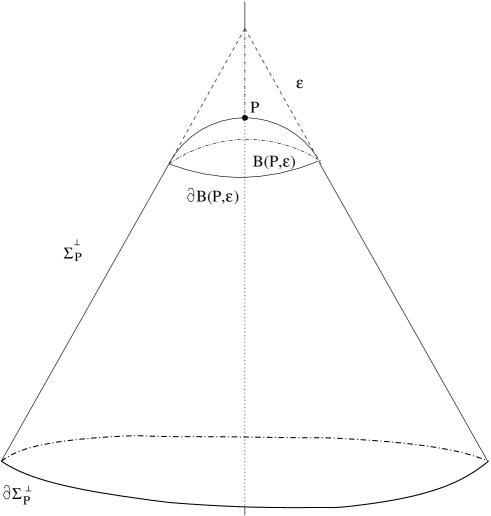
Figure 2: The normal section $\Sigma^{\perp}_{P}$. The cone has been regularised here by an axially symmetric metric. Note that the first integral in (73) refers to the boundary shrinking to the tip of the cone whereas the latter to the smoothed out charge at $P$. Their difference gives the geometric distributional charge.

We can now write the matching conditions for a brane of arbitrary codimension,

$$\sum_{k=\left[N/2\right]}^{\left[(D-1)/2\right]}\alpha_{k}\left[q_{(N,k)\mu}\right](P)=-2S_{\mu}{}^{\nu}(P)\theta^{\star{//}}_{\nu}\,,$$ (72)

where

$$\left[q_{(N,k)\mu}\right]\equiv\lim_{\int_{\partial\Sigma_{P}^{\perp}}\rightarrow 0}(-1)^{D-N-1}\int_{\partial\Sigma_{P}^{\perp}}n_{N}^{*}\,\sigma_{(N,k)\mu}-q_{(N,k)\mu}(P)\neq 0$$ (73)

is the discontinuity in the charge when passing from the brane to the bulk and the potentials $\sigma_{(N,k)\mu}$ are given in (62). The first and second terms in (73) are of different nature if and only if the RHS of (72) is non-vanishing. In loose terms the former integral takes account of the Dirac singularity whereas the latter is the charge of the “smoothed out defect”. For the case of the cosmic string, as we will see in the next section, the former is the cone’s exterior geometry giving the string defect $\beta$, whereas the latter is the charge of the smoothed out geometry giving simply 1 (see figure (2)). We remind the reader that $N$ is the codimension of the brane, $k$ is the rank of the Lovelock density (with $k=1$ for the Einstein term) and $D$ is the spacetime dimension.

In the next section, we will put the matching conditions to application, starting with known cases and then focusing on cases of physical interest. The important point to remember is that the potential (62) is given in terms of the Chern-Simons forms (60), which are integrated out over the sphere, and a parallel part $\sigma^{{//}}_{(N,k)\mu}$, which will end up giving the equations of motion for the brane.

5 Action and equations of motion for a brane of arbitrary codimension

Let us now analyse the matching conditions (72) at hand. In view of the discontinuity (73), we need to get a jump from the potentials $\sigma_{(N,k)\mu}$ as we shrink the boundary $\partial\Sigma_{P}^{\perp}$ to $P$. Given the decomposition of $\sigma_{(N,k)\mu}$ into normal and parallel components (62), there are a priori three seperate ways to achieve this:

• (I) the parallel components $\sigma^{{//}}_{(N,k)\mu}$, (63), are smooth and the jump thus comes from the perpendicular part of $\sigma_{(N,k)\mu}$, ie (61). We refer to this case as the purely topological case for reasons that will become apparent in a moment.

• (II) the perpendicular part of $\sigma_{(N,k)\mu}$, ie (61), is smooth and the jump originates solely from $\sigma^{{//}}_{(N,k)\mu}$, (63). This is always the case for matching conditions involving hypersurfaces, $N=1$, [1],[41],[42]

• (III) both parts in (62) are discontinuous. For $N=2$ and $D=6$, this case yields the results of [21].

For (I), a discontinuity in the perpendicular components originates from the Chern-Simons forms, (60). This means, according to (68), that the area of the boundary surrounding the normal section, ie the limit of the integral in (73), must be different from the charge at $P$, which is proportional to $\mbox{Area}({\mathbb{S}}_{N-1})$, (68). Therefore, we must have a topological defect at the location of $\Sigma$, permitting the discontinuity in (73). For codimension 2, $N=2$, the topological defect is nothing but the conical deficit obtained by reducing the circumference of ${\mathbb{S}}_{1}$ by $2\pi(1-\beta)$. Similarly, a topological defect for any $N$ can simply be realised by cutting a solid angle $(1-\beta)\mbox{Area}({\mathbb{S}}_{N-1})$ from ${\mathbb{S}}_{N-1}$ , as one does for the far field of a global monopole, $N=3$, in Einstein gravity (see for example [43]). For the topological case, using (73), the matching conditions read

$$(1-\beta(P))\mbox{Area}({\mathbb{S}}_{N-1})\sum_{k=\left[N/2\right]}^{\left[(D-1)/2\right]}(-1)^{N}\alpha_{k}D_{(N,k)}\sigma^{{//}}_{(N,k)\mu}(P)=-2S_{\mu}{}^{\nu}(P)\theta^{\star{//}}_{\nu}\,,$$ (74)

where the equations of motion are essentially given by the geometric terms (63) and $\beta$ a priori depends on the position $P$ along the brane. This is clearly the simplest of cases and the one preserving the most mathematical regularity for the spacetime metric, since both the induced and extrinsic brane geometry are regular at $P$. We will argue later on in this section that the topological matching conditions are the ones adequate for even codimension branes.

In (II) on the contrary, the topology is trivial and the discontinuity originates from the parallel components (63). In particular, given that the equations of motion in the bulk are of second order in the metric and that the metric is thus necessarily continuous at $P$, the discontinuity can only originate from the extrinsic curvature 1-forms (16). This is always the case with matching conditions involving hypersurfaces, $N=1$, since there is no geometry in the normal sections, specifically $\Pi^{\perp}_{(1,0)}=1$. The matching conditions read,

$$\mbox{Area}({\mathbb{S}}_{N-1})\sum_{k=\left[N/2\right]}^{\left[(D-1)/2\right]}(-1)^{N}\alpha_{k}D_{(N,k)}\,\left(\lim_{\int_{\partial\Sigma_{P}^{\perp}}\rightarrow 0}\sigma^{{//}}_{(N,k)\mu|\partial\Sigma_{P}{{}^{\perp}}}-\sigma^{{//}}_{(N,k)\mu}(P)\right)=2S_{\mu}{}^{\nu}(P)\theta^{\star{//}}_{\nu}\,.$$ (75)

In (III), the jump comes from a global discontinuity in (62). Note that this case is possible only because the perpendicular (61) and the parallel components (63) in (62) combine to give a total differential obeying (56). This permits us to consider distributions in the first place (see Appendix C). The importance of this case will become manifest in the next section, when treating specific examples for odd codimension defects.

As a first step, we now make the connection to known boundary conditions for Einstein and Gauss-Bonnet gravity, starting with codimension $N=1$. The only normal induced Chern-Simons form in (60) is the trivial one, $\Pi^{\perp}_{(1,0)}=1$, and, as we mentioned above, a charge can only originate from a discontinuity in the parallel part, case (II). Replacing directly into (62) and using (29) and (37), we get in turn for the Einstein and Gauss-Bonnet terms,

$$\sigma^{//}_{(1,1)\mu} = 2\,{\cal{K}}^{\nu}_{{//}N}\wedge\theta^{\star{//}}_{\mu\nu}=-2\,(K^{\nu}_{\mu}-\delta^{\nu}{}_{\mu}K)\theta^{\star{//}}_{\nu}$$

$$\sigma^{{//}}_{(1,2)\mu} = 4\,{\cal{K}}^{\nu}_{{//}N}\wedge\left(\Omega^{\rho\lambda}_{{//}}-\frac{1}{3}{\cal{K}}^{\rho}_{{//}N}\wedge{\cal{K}}^{\lambda}_{{//}N}\right)\wedge\theta^{\star{//}}_{\mu\nu\rho\lambda}$$ (76)

$$= -4(3J_{\mu}^{\nu}-J\delta_{\mu}^{\nu}-2P^{\nu}_{\;\;\lambda\rho\mu}K^{\lambda\rho})\theta^{\star{//}}_{\nu}\,,$$

where we have set

$$J_{\mu\nu}=\frac{1}{3}(2KK_{\mu\lambda}K^{\lambda}{}_{\nu}+K_{\lambda\rho}K^{\lambda\rho}K_{\mu\nu}{}-2K_{\mu\lambda}K^{\lambda\rho}K_{\rho\nu}-K^{2}K_{\mu\nu}),$$

$$P_{\mu\nu\lambda\rho}=R_{\mu\nu\lambda\rho}+2R_{\nu[\lambda}g_{\rho]\mu}-2R_{\mu[\lambda}g_{\rho]\nu}+Rg_{\mu[\lambda}g_{\rho]\nu}$$

and we have dropped the label $N$ for the extrinsic curvature components. Replacing into the matching conditions (75) and taking the corresponding left and right limits (the charges (68) cancel out here), one gets the well-known junction conditions for Einstein [1] and Einstein-Gauss-Bonnet gravity [41, 42]. Not surprisingly, the equations of motion can be derived from the boundary action, after variation with respect to the induced frame $\theta^{\nu}$ on the left and right side of the brane. In differential form language the action is obtained trivially from (5),

$$S_{\Sigma}=2\alpha_{1}\int_{\Sigma}{\cal{K}}^{\nu}_{{//}N}\wedge\theta^{\star{//}}_{\nu}+4\alpha_{2}\int_{\Sigma}{\cal{K}}^{\nu}_{{//}N}\wedge\left(\Omega^{\rho\lambda}_{{//}}-\frac{1}{3}{\cal{K}}^{\rho}_{{//}N}\wedge{\cal{K}}^{\lambda}_{{//}N}\right)\wedge\theta^{\star{//}}_{\nu\rho\lambda}$$ (77)

and agrees with the Gibbons-Hawking [36] and Myers [34] boundary terms (44), (45).

We now consider the codimension 2 case, $N=2$. Here, things are quite different for the potentials of the charged exact forms (69) coming from the Einstein and Gauss-Bonnet terms,

$$\sigma_{(2,1)\mu}^{//} = 2\theta^{\star{//}}_{\mu},\qquad\sigma_{(2,2)\mu}^{//}=4{\cal{R}}_{{//}}^{\nu\rho}\wedge\theta^{\star{//}}_{\mu\nu\rho}\,.$$ (78)

The charges are trivially obtained from (68) and they involve $\Pi^{\perp}_{(2,0)}$. This time, the normal section has the topology of the unit 2-dimensional disk. What is particularily interesting for the comprehension of the matching conditions is that all three cases are possible for the Gauss-Bonnet potential term. Indeed, starting with the Einstein term, we see from (78) that since the tangent frame is smooth, the associated charge (68) can only be purely topological,

$$\left[q_{(2,1)\mu}\right]=4\pi(1-\beta)\,\theta^{\star{//}}_{\mu}\,,$$ (79)

and refers to the conical deficit of $\Sigma_{P}^{\perp}$ -in particular, this yields the matching conditions for a cosmic string in $D=4$. For the Gauss-Bonnet term, it is useful to decompose the projected curvature operator ${\cal{R}}_{{//}}^{\nu\rho}$ using Gauss relation (29),

$$\sigma^{{//}}_{(2,2)\mu}=4(\Omega_{{//}}^{\nu\rho}\wedge\theta^{\star{//}}_{\mu\nu\rho}-{\cal{K}}_{{//}}^{\nu I}\wedge{\cal{K}}_{{//}I}^{\rho}\wedge\theta^{\star{//}}_{\mu\nu\rho})\,,$$ (80)

where, note the summation over the normal index $I$. Since the induced curvature 2-form $\Omega_{{//}}^{\nu\rho}$ of $\Sigma$ is smooth by hypothesis, the charge is topological for the first term in the RHS of (80). For the second term however, one can ask for a jump of the whole term, yielding the most general contribution in (73),

$$\left[q_{(2,2)\mu}\right] = 8\pi(1-\beta)\,\Omega^{\nu\rho}_{{//}}\theta^{\star{//}}_{\mu\nu\rho}+8\pi\,\left[\tilde{\beta}\,{\cal{K}}^{\lambda I}_{{//}}\wedge{\cal{K}}^{\rho}_{{//}I}\wedge\theta^{\star{//}}_{\mu\lambda\rho}\right]$$ (81)

$$= -16\pi(1-\beta)G_{\mu}^{(ind)\nu}\theta^{\star{//}}_{\nu}+16\pi\,\left[\tilde{\beta}\,W_{\mu}^{\nu}\right]\theta^{\star{//}}_{\nu}\,,$$ (82)

where we have introduced the tangent induced Einstein tensor $G_{\mu\nu}^{(ind)}$, and we have set [21], [26],

$$W_{\mu}^{\lambda}=K^{\nu I}_{\mu}K^{\lambda}_{\nu I}-K^{I}K^{\lambda}_{\mu I}+\frac{1}{2}\delta^{\lambda}{}_{\mu}\left(K_{I}K^{I}-K^{\nu I}_{\rho}K^{\rho}_{\nu I}\right)$$ (83)

and

$$\tilde{\beta}\equiv\left\{\begin{array}[]{cc}1&\mbox{on the brane}\\ \beta&\mbox{in the bulk}\end{array}\right.$$ (84)

This obviously corresponds to the 3rd bullet point. The matching conditions (72) in this case read,

$$2\pi\,(1-\beta(P))\left\{-\alpha_{1}h_{\mu\nu}+4\alpha_{2}G^{(ind)}{}_{\mu\nu}\right\}-8\pi\,\alpha_{2}\,\left[\tilde{\beta}W_{\mu\nu}\right]=S_{\mu\nu}\,.$$ (85)

This result generalises that derived in [21] (see also [26]), where axial symmetry and the vanishing of the extrinsic curvature $K^{\mu}_{\nu N}$ on the brane were assumed. These matching conditions ask for a singular behaviour of the extrinsic curvature terms, as well as a topological charge. This is rather constraining and mathematically not necessary. Let us now relax either of these assumptions.

If $\beta=1$, ie there is no topological charge at all, the Einstein term yields no contribution and the matching conditions are very much reminiscent of those for hypersurfaces,

$$-8\pi\,\alpha_{2}\,\left[W_{\mu\nu}\right]=S_{\mu\nu}\,.$$ (86)

This is of course bullet point 1. Note that this case does not allow at all for matching conditions for Einstein gravity and can therefore be rejected as unphysical. However, let us suppose now that the extrinsic curvature terms are regular, ie $W_{\mu\nu}$ is continuous, and therefore the charge is only topological. Note then that $W_{\mu\nu}$ on the brane only depends on the normal extrinsic curvature, ie we set $I=N$ in (83), since, by regularity, any angular extrinsic curvature terms are zero on the brane’s location. This yields the most natural case that agrees, on the one hand, with the cosmic string calculation in Einstein gravity and, on the other hand, with maximal regularity of the spacetime metric. We obtain,

$$2\pi\,(1-\beta(P))\left\{-\alpha_{1}h_{\mu\nu}+4\alpha_{2}G_{\mu\nu}^{(ind)}+4\,\alpha_{2}\,W_{\mu\nu}\right\}=S_{\mu\nu}(P)\,.$$ (87)

Both for (85), [21], as well as for the topological matching condition (87), we see that the bulk Einstein term, $k=1$, only allows for a pure tension brane, ie for a cosmological constant term in the matching conditions, while the Gauss-Bonnet term allows for arbitrary matter with an induced Einstein equation on the brane [21]. Some comments are now in order concerning the bulk degree of freedom $\beta=\beta(P)$. In particular, note that the matching conditions, ie the distributional part of the Lovelock tensor, do not permit us to evaluate this function. The remaining bulk equations have to be used in order to do so. Indeed, we emphasize that here, we have only calculated the distributional part of the Lovelock equations which yield the matching conditions. This, of course, is not sufficient to guarantee a full solution of the bulk field equations. Nevertheless, already at the level of (87), the effect of this scalar function is similar to a Brans-Dicke field, varying the coupling of gravity to matter on the brane and thus breaking the equivalence principle for a brane observer. Such effects are heavily constrained by local gravity experiments (see [24]), where stringent observational bounds can be put on the variation in time of the function $\beta$. One also expects that, if $\beta$ is varying, the brane will be radiating gravitational waves into the bulk . These are very interesting issues which demand further work, but in order to present the matching conditions here, let us suppose for what follows that $\beta$ is constant. In this case, there is an additional remarkable property of the topological matching conditions, which is due to the fact that the extrinsic geometry is regular. The equations of motion actually originate from a simple action involving induced and extrinsic quantities over $\Sigma$. In other words, the degrees of freedom associated to the normal section are completely integrated out, giving an exact action for the brane’s motion. In differential form language, it is straightforward to read off the langrangian density in question. Literally, take out the free index for the charge in (81) and use Gauss (30) to get,

$$S_{\Sigma}^{(p=3,n=1)} = 4\pi(1-\beta)\,\int_{\Sigma}\left(\alpha_{1}\theta^{\star//}+2\alpha_{2}(R^{\nu\rho}_{{//}}\wedge\theta^{\star{//}}_{\nu\rho})\right)+\int_{\Sigma}{\cal{L}}_{matter}$$ (88)

$$= 4\pi(1-\beta)\int_{\Sigma}\sqrt{-h}\;\left(\alpha_{1}+2\alpha_{2}(R^{ind}-K^{2}+K_{\mu\nu}^{2})\right)+\int_{\Sigma}{\cal{L}}_{matter}\,,$$

ie the cosmological constant plus Einstein-Hilbert action with an extrinsic curvature term. In other words, the only bulk quantity entering in the equations of motion is the extrinsic curvature of the surface, giving a matter like component in the action. If this is set to zero, ie when $\Sigma$ is totally geodesic, we have a cosmological constant plus Einstein gravity as an exact equation of motion for the brane. Note that the overall mass scale of the integrated 4-dimensional theory is free and is set by the topological defect $\beta$. Furthermore, we see a kind of pattern appearing between the Lovelock densities in the bulk and the reduced ones on the brane. This “reduction”, from Gauss-Bonnet in the bulk ($k=2$) to Einstein gravity on the brane and from Einstein in the bulk ($k=1$) to a cosmological term on the brane, is a general feature that applies to higher order Lovelock densities and higher even codimension. The origin is again topological as we will see now.

Indeed, let us now assume that $N=2n$ is even. Let us also suppose that we have a p-brane, ie $D-2n=p+1$. This means, (64), that the Lovelock rank must satisfy

$$n\leq k\leq n+\left[{p\over 2}\right]\,.$$ (89)

For a 1-brane, we have $k=n$, ie only a cosmological constant term $\tilde{k}=k-n=0$,

$$S^{(p=1,n)}_{\Sigma}=(1-\beta)\mbox{Area}({\mathbb{S}}_{2n-1}))\,\int_{\Sigma}\tilde{\alpha}_{n}\sqrt{-h}\,,$$ (90)

where we have set $\tilde{\alpha}_{k}=D_{(2n,k)}\alpha_{k}$ and have taken $\beta$ constant. In turn, for a ($p=3$)-brane embedded in higher codimension, $n>1$, we have $k=n$ and $k=n+1$. The topological matching condition (74) gives

$$\tilde{\alpha}_{n}\theta_{\mu}^{\star//}+\tilde{\alpha}_{n+1}({\cal{R}}_{{//}}^{\nu\rho}\wedge\theta^{\star{//}}_{\mu\nu\rho}+{\cal{K}}_{{//}N}^{\nu}\wedge{\cal{K}}_{{//}N}^{\rho}\wedge\theta^{\star{//}}_{\mu\nu\rho})=\frac{2}{(\beta-1)\mbox{Area}({\mathbb{S}}_{N-1})}S_{\mu}{}^{\nu}(P)\theta^{\star{//}}_{\nu}\,.$$ (91)

This equation tells us a remarkable property of 3-branes, for if we now use Gauss equation (29), the “squared” extrinsic curvature form cancels out leaving Einstein’s equation with a cosmological constant! The 3-brane action is simply

$$S_{\Sigma}^{(p=3,n>1)} = \mbox{Area}({\mathbb{S}}_{N-1})(1-\beta)\int_{\Sigma}\sqrt{-h}\;\left(\tilde{\alpha}_{n}+\tilde{\alpha}_{n+1}R^{ind}\right)+\int_{\Sigma}{\cal{L}}_{matter}$$ (92)

and is valid as long as codimension is even and $n>1$. The Planck scale. on the 3-brane is

$$M_{Pl}^{2}=(1-\beta)\mbox{Area}({\mathbb{S}}_{N-1})\tilde{\alpha}_{n+1}\,.$$ (93)

Note that only the topological matching conditions exist here, for there are no extrinsic curvature terms at all! In a nutshell, we have a dimensional reduction from the Euler densities of the bulk to the induced Euler densities on the brane. This has two important consequences. If we are for example in D=10 dimensions, it is the highest order Lovelock density, $k=4$, that precicely gives us the Einstein contribution on the brane. In turn, the $k=3$ density will give an induced cosmological constant. The bulk Einstein term, for example, contributes nothing since it cannot carry a Dirac charge! We obtain the most general dynamics as far as the induced geometry of the brane is concerned. The order of the induced Lovelock density is simply $\tilde{k}=k-n$ and obeys (89)

$$0\leq\tilde{k}\leq\left[{p\over 2}\right]\,.$$ (94)

It turns out, [44], that the extrinsic curvature terms identically drop out, leaving a pure induced Lovelock brane action for any p-brane, as long as

$$\left[{p\over 2}\right]+1\leq n\,.$$ (95)

This means that the worldvolume dimension is less than or equal to the brane’s codimension. If we now consider a 5-brane, we have $k=n$ which gives a cosmological constant term ($\tilde{k}=0$), $k=n+1$ which gives the induced Einstein term and no extrinsic curvature corrections ($\tilde{k}=1$), and in addition $k=n+2$ which yields a Gauss-Bonnet dynamical term on the brane ($\tilde{k}=2$). Explicitely, for $k=n+2$, we have the potentials

$$\sigma_{(2,3)\mu}^{//} = {\cal{R}}^{\nu\rho}_{{//}}\wedge{\cal{R}}^{\lambda\sigma}_{{//}}\wedge\theta^{\star{//}}_{\mu\nu\rho\lambda\sigma}$$ (96)

$$\sigma_{(4,4)\mu}^{//} = \left(\textstyle{1\over 2}{\cal{R}}^{\nu\rho}_{{//}}\wedge{\cal{R}}^{\lambda\sigma}_{{//}}+{\cal{R}}^{\nu\rho}_{{//}}\wedge{\cal{K}}^{\lambda}_{N//}\wedge{\cal{K}}^{\sigma}_{N//}\right)\wedge\theta^{\star{//}}_{\mu\nu\rho\lambda\sigma}\,,$$ (97)

which are valid for $n=1$ and $n=2$ respectively. Note then, that the first term in each sum yields the Gauss-Bonnet tensor once we trade ${\cal{R}}^{\nu\rho}_{{//}}$ for the induced curvature 2-form $\Omega^{\nu\rho}_{{//}}$ by Gauss equation. For $n\geq 3$ (95), the extrinsic curvature terms drop out, giving us the induced Gauss-Bonnet tensor on the brane,

$$\sigma_{(2n,n+2)\mu}^{//} = \textstyle{1\over 2}\left({\cal{R}}^{\nu\rho}_{{//}}\wedge{\cal{R}}^{\lambda\sigma}_{{//}}+2{\cal{R}}^{\nu\rho}_{{//}}\wedge{\cal{K}}^{\lambda}_{N//}\wedge{\cal{K}}^{\sigma}_{N//}+\right.$$ (98)

$$+ \left.{\cal{K}}^{\nu}_{N//}\wedge{\cal{K}}^{\rho}_{N//}\wedge{\cal{K}}^{\lambda}_{N//}\wedge{\cal{K}}^{\sigma}_{N//}\right)\wedge\theta^{\star{//}}_{\mu\nu\rho\lambda\sigma}$$

$$= \frac{1}{2}\Omega^{\nu\rho}_{{//}}\wedge\Omega^{\lambda\sigma}_{{//}}\wedge\theta^{\star{//}}_{\mu\nu\rho\lambda\sigma}\,.$$

Therefore, the 5-brane action reads

$$S^{(p=5,n\geq 3)}_{\Sigma} = \mbox{Area}({\mathbb{S}}_{N-1})(1-\beta)\int_{\Sigma}\sqrt{-h}\left(\tilde{\alpha}_{n}+\tilde{\alpha}_{n+1}R^{ind}\right.$$ (99)

$$\left.+\tilde{\alpha}_{n+2}(R^{\mu\nu\lambda\rho}_{(ind)}R^{(ind)}_{\mu\nu\lambda\rho}-4R_{(ind)}^{\mu\nu}R^{(ind)}_{\mu\nu}+R_{(ind)}^{2})\right)+\int_{\Sigma}{\cal{L}}_{matter}\,,$$

ie the general Lovelock action for a 5-brane. This is a general feature for even codimensions: Any p-brane of even codimension, embedded in a $D\geq 2(p+1)-$dimensional spacetime, obeys exactly the induced Lovelock equations! At the level of zero thickness, there are no degrees of freedom originating from the bulk spacetime apart from the topological charge $\beta$. In particular, an observer on a 3-brane will have no way of knowing that he is embedded in a 10 dimensional spacetime, up to finite width corrections. Lastly, we argue that in the case of even co-dimension one should consider topological matching conditions. Indeed the first reason as we emphasized earlier on is mathematical regularity. There is no reason to impose discontinuous geometric quantities if the Lovelock equations do not explicitely demand it. The second reason comes from the nice physical properties of the topological conditions. As we saw we can write down an induced action for the brane which remarkably integrates out all the bulk degrees of freedom. In particular, if condition (95) is satisfied no extrinsic curvature terms appear in the actual matching conditions and therefore only topological matching conditions are possible.

For odd codimension, $N=2n+1$, we will concentrate only on the general matching conditions (72). This is motivated by the maximally symmetric example we will discuss in the next section. From (64), we have

$$n+1\leq k\leq n+\left[{p+1\over 2}\right]\,.$$ (100)

We will always have odd powers of the extrinsic curvature form ${\cal{K}}$ in the matching conditions, so there will never be an induced Einstein term on its own. This is to be expected from the junction conditions for hypersurfaces. When $k=n+\left[{p+1\over 2}\right]$, ie $k$ has its maximal value, we have $0\leq j\leq$min$(n,\left[{p+1\over 2}\right])$. Depending again on the magnitude of $n$, we will pick up all or some of the geometric quantities. For the case of a 3-brane of codimension $N=3$, the relevant charges in (72) are

$$q_{(2n+1,n+1)\mu}=\left[\tilde{\beta}{\cal{K}}^{\rho}_{N//}\right]\wedge\theta^{\star//}_{\mu\rho}$$ (101)

$$q_{(n=0,2)\mu}=q_{(n=1,3)\mu}=\left[\tilde{\beta}{\cal{R}}^{\nu\sigma}_{//}\wedge{\cal{K}}^{\rho}_{N//}\right]\wedge\theta^{\star//}_{\mu\nu\sigma\rho}\,,$$ (102)

whereas if $N>3$, we obtain an additional term (101) for $k=n+2$, yielding

$$q_{(n>1,n+2)\mu}=\left(\left[\tilde{\beta}{\cal{R}}^{\nu\sigma}_{//}\wedge{\cal{K}}^{\rho}_{N//}\right]+{2\over 3}\left[\tilde{\beta}{\cal{K}}^{\nu}_{N//}\wedge{\cal{K}}^{\sigma}_{N//}\wedge{\cal{K}}^{\rho}_{N//}\right]\right)\wedge\theta^{\star//}_{\mu\nu\sigma\rho}\,,$$ (103)

which is just an extension of the Myers boundary term [34], but for a 3-brane. In other words, if

$$\left[{p+1\over 2}\right]\leq n$$ (104)

is satisfied, then the matching conditions will only involve the dimensional continuation of Chern-Simons forms on $\Sigma$.

6 Maximally symmetric 1-branes of higher codimension

The matching conditions we discussed in all generality in the previous section are only necessary conditions for the existence of higher codimension Dirac branes. Indeed, the matching conditions only depend on the $\mu\nu$-components of the Lovelock equations (48) and unlike hypersurfaces do not give Cauchy type conditions for the local reconstruction of the bulk spacetime. In this section, we construct simple spacetime solutions that carry a brane of Dirac charge. We concentrate on cases of maximal symmetry both for the bulk and for the brane. Such solutions, as we will argue, do not exist for Einstein gravity.

6.1 The codimension 3 case

Consider a maximally symetric 1-brane embedded in a 5-dimensional static spacetime of axial symmetry about the brane. We call $r$, the proper distance to the brane. Then, let $A(r)$ be the brane warp factor and $L(r)$ the size of the 2-spheres. We thus have

$$ds^{2}=A^{2}(r)\left(-dt^{2}+e^{2kt}\,dz^{2}\right)+dr^{2}+L^{2}(r)\left(\beta^{-2}\,d\theta^{2}+\sin^{2}\theta\,d\phi^{2}\right)\,.$$ (105)

Note that in order for the induced geometry of the brane to be adS, one can Wick rotate $t$ and $z$ in (105), to obtain a flat slicing of adS. The stress-energy tensor of the brane located at $r=0$, is taken to be

$$T^{t}{}_{t}=T^{z}{}_{z}=\sigma\,\frac{\beta\delta(r)}{4\pi L^{2}}\,,$$ (106)

with all the other components vanishing. We have odd codimension and, since $n=1$, we have Lovelock density up to $k=2$. From (100), we know that the only possible charge comes from the Gauss-Bonnet term ${\cal{L}}_{(2)}$, whose components read

$$H^{t}{}_{t}=H^{z}{}_{z} = \frac{4}{AL^{2}}\hat{f}^{\prime}+\frac{4}{A}\left[f\right]{\delta(r)\over L^{2}}$$ (107)

$$H^{r}{}_{r} = \frac{4L^{\prime 2}\left(k^{2}-3A^{\prime 2}\right)+4\beta^{2}\,\left(A^{\prime 2}-k^{2}\right)}{A^{2}L^{2}}$$ (108)

$$H^{\theta}{}_{\theta}=H^{\phi}{}_{\phi} = 4\frac{\left(\left(k^{2}-A^{\prime 2}\right)L^{\prime}\right)^{\prime}}{A^{2}L}\,,$$ (109)

with $f=A^{\prime}\left(\beta^{2}-L^{\prime 2}\right)$. As usual, the square brackets denote the jump and $\hat{\mbox{ }}$ the smooth part. Given (107), we can get a Dirac distribution centered on the world-sheet, provided that $f$ is discontinuous at $r=0$. To make things simple, let us first consider a pure Gauss-Bonnet equation, $H^{A}_{B}=0$, since this is the only term that will provide a charge. The general solution reads,

$$L(r)=lr\,,\quad A(r)=ar+r_{0}\,.$$ (110)

There are now at least two different ways, using the spacetime topology, to obtain a distributional charge. We either introduce a uniform solid angle defect (like the global monopole) for the entire spherical section or we introduce a defect angle in the direction of the axis $\theta=0$. The former is achieved by setting $\beta=1$ in (105) and $l\neq 1$. However, the solutions (110) generically have a curvature singularity as $r\rightarrow 0$, as can be seen from the divergence of the Ricci scalar,

$$R\sim-8\,\frac{A^{\prime}}{A}\frac{L^{\prime}}{L}+2\,\frac{\left(\beta^{2}-L^{\prime 2}\right)}{L^{2}}\,.$$ (111)

In order to avoid such a singularity in the vicinity of the brane, we consider the latter case,

$$L^{\prime}\sim\beta\quad\mbox{and}\quad A^{\prime}\sim 0\,,$$ (112)

as $r$ goes to zero and therefore

$$f(r)=\left\{\begin{array}[]{cc}0&\mbox{if $r=0^{+}$}\\ a(1-\beta^{2})&\mbox{if $r=0$}\end{array}\right.$$ (113)

to get the desired Dirac distribution. Note here that the matching conditions have to be mixed (III)! They cannot be only topological for then we would have a singular spacetime metric. Let us also point out that the matching conditions do not suffice to guarantee the good behaviour of the spacetime metric. Replacing directly into (53), we get in turn,

$$\alpha_{2}\int_{\Sigma_{P}}{dr\,d\theta\,d\phi L^{2}\sin\theta\over\beta}[A^{\prime}(\beta^{2}-L^{\prime 2})]{\delta(r)\over AL^{2}}=-{4\pi\alpha_{2}\over\beta r_{0}}a(\beta^{2}-1)={\sigma}\,,$$ (114)

where the powers of $L$ drop out, giving the usual 1-dimensional Dirac distribution. In the end,

$$4\pi\alpha_{2}{a\over\beta r_{0}}(1-\beta^{2})=\sigma$$ (115)

and we have a pure Gauss-Bonnet 1-brane of codimension 3. We should note however at this point that our construction introduces a conical singularity along the polar axis $\theta=0$, not only at $r=0$.

Now that we have understood how to build a Dirac distribution out of the Gauss-Bonnet term, we can extend the simple calculation to the full Lovelock theory, with field equations

$$\Lambda\delta^{A}{}_{B}+\zeta\,G^{A}{}_{B}+\alpha\,H^{A}{}_{B}=0\,.$$ (116)

We get in the bulk,

$$\Lambda + \zeta\,\left(\frac{A^{\prime\prime}}{A}+2\frac{A^{\prime}}{A}\frac{L^{\prime}}{L}+2\frac{L^{\prime\prime}}{L}+\frac{L^{\prime 2}-\beta^{2}}{L^{2}}\right)+4\alpha\,\frac{\left(A^{\prime}\left(\beta^{2}-L^{\prime 2}\right)\right)^{\prime}}{AL^{2}}=0$$ (117)

$$\Lambda + \zeta\,\left(\frac{A^{\prime 2}-k^{2}}{A^{2}}+\frac{L^{\prime 2}-\beta^{2}}{L^{2}}+4\frac{A^{\prime}}{A}\frac{L^{\prime}}{L}\right)+4\alpha\,\frac{L^{\prime 2}\left(k^{2}-3A^{\prime 2}\right)+\beta^{2}\,\left(A^{\prime 2}-k^{2}\right)}{A^{2}L^{2}}=0$$ (118)

$$\Lambda + \zeta\,\left(2\frac{A^{\prime\prime}}{A}+\frac{L^{\prime\prime}}{L}+\frac{A^{\prime 2}-k^{2}}{A^{2}}+2\frac{A^{\prime}}{A}\frac{L^{\prime}}{L}\right)+4\alpha\,\frac{\left(\left(k^{2}-A^{\prime 2}\right)L^{\prime}\right)^{\prime}}{A^{2}L}=0$$ (119)

which admits the following solution,

$$ds^{2}=k^{2}r_{0}^{2}\,\cos^{2}\left(\frac{r}{r_{0}}\right)\,\left(-dt^{2}+e^{2kt}dz^{2}\right)+dr^{2}+r_{0}^{2}\beta^{2}\,\sin^{2}\left(\frac{r}{r_{0}}\right)\,\left(\beta^{-2}d\theta^{2}+\sin^{2}\theta\,d\phi^{2}\right)\,,$$ (120)

with

$$r_{0}^{2}=\frac{\zeta\mp\sqrt{\zeta^{2}+\frac{4\alpha\Lambda}{3}}}{\Lambda/3}\,.$$ (121)

This is a slicing of de-Sitter spacetime for $\Lambda>0$. The flat space limit is obtained by taking $k\sim 1/r_{0}$ and $r_{0}\rightarrow\infty$. Then, spacetime is locally flat, exhibiting only a conical singularity at $r=0$, as for a straight cosmic string [45]. The negative cosmological constant case is simply

$$ds^{2}=k^{2}r_{0}^{2}\,\cosh^{2}\left(\frac{r}{r_{0}}\right)\,\left(dz^{2}-e^{2kz}dt^{2}\right)+dr^{2}+r_{0}^{2}\beta^{2}\,\sinh^{2}\left(\frac{r}{r_{0}}\right)\,\left(\beta^{-2}d\theta^{2}+\sin^{2}\theta\,d\phi^{2}\right)\,,$$ (122)

with

$$r_{0}^{2}=\frac{\zeta\mp\sqrt{\zeta^{2}+\frac{4\alpha\Lambda}{3}}}{-\Lambda/3}\,.$$ (123)

Now, we can use the same method as in the pure Gauss-Bonnet case (113) to obtain matching conditions for distributional matter (106). Going through all the terms in the field equations, we see again that the only term carrying a distributional charge is $f$ (113). Terms originating from the Einstein tensor, like ${L^{\prime\prime}\over L}$, could carry a 2 dimensional Dirac charge but not a 3 dimensional one. We have therefore constructed an Einstein-Gauss-Bonnet 1-brane of codimension 3, embedded in a constant or zero curvature bulk. The matching conditions are again given by (115).

6.2 The codimension 4 case

We now consider a 1-brane of codimension 4 as a solution of pure Gauss-Bonnet gravity. The 6 dimensional space-time metric with axial symmetry reads,

$$ds^{2} = A^{2}(r)\left(-dt^{2}+e^{2kt}\,dz^{2}\right)$$ (124)

$$+dr^{2}+L^{2}(r)\left(\beta^{-2}\,d\theta^{2}+\gamma^{-2}\,\sin^{2}\theta\,d\phi^{2}+\sin^{2}\theta\,\sin^{2}\phi\,d\psi^{2}\right)\,,$$

and we assume the presence of an energy-momentum tensor,

$$T^{t}{}_{t}=T^{z}{}_{z}=\sigma\frac{\beta\gamma\delta(r)}{2\pi^{2}L^{3}}\,,$$ (125)

As for the codimension 3 case, $L(r)\sim lr$ as $r$ goes to zero and the metric (124) is generically singular at $r=0$,

$$R\sim-12\,\frac{A^{\prime}}{A}\,\frac{L^{\prime}}{L}+2\,\frac{3L^{\prime 2}-2\beta^{2}-\gamma^{2}+3\left(\beta^{2}-L^{\prime 2}\right)\cos^{2}\theta}{L^{2}\left(\cos^{2}\theta-1\right)}\,.$$ (126)

The non-singular bulk solutions therefore have to satisfy $\gamma^{2}=\beta^{2}$ and

$$L^{\prime 2}\sim\beta^{2}\quad\mbox{and}\quad A^{\prime}\sim 0\,,$$ (127)

as $r$ goes to zero, which imposes the topology of a conical deficit angle. However, for codimension 4, a jump in $A^{\prime}$ does not give rise to a Dirac distribution since the second derivatives of $A$ only appear in terms of order $L^{-2}$ in the components of the Gauss-Bonnet tensor. We therefore set $A\sim 1$ as $r$ goes to zero. In the vicinity of the brane, we thus obtain

$$H^{t}{}_{t}=H^{z}{}_{z} \sim \frac{4}{L^{3}}\hat{f}^{\prime}+\frac{4\delta(r)}{L^{3}}\left[f\right]$$ (128)

$$H^{r}{}_{r} \sim 4\frac{k^{2}\left(L^{\prime 2}-\beta^{2}\right)}{L^{2}}$$ (129)

$$H^{\theta}{}_{\theta}=H^{\phi}{}_{\phi}=H^{\psi}{}_{\psi} \sim \frac{4k^{2}\left(L^{\prime 2}-\beta^{2}\right)}{L^{2}}-8k^{2}\frac{L^{\prime\prime}}{L}\,,$$ (130)

where we have set $f=(3\beta^{2}-L^{\prime 2})L^{\prime}$. The jump of this function at the origin,

$$f(r)=\left\{\begin{array}[]{cc}2\beta^{3}&\mbox{if $r=0^{+}$}\\ 3\beta^{2}-1&\mbox{if $r=0$}\end{array}\right.$$ (131)

allows for the topological matching condition

$$\sigma={2\pi^{2}\over\beta^{2}}(1-\beta)(1+\beta-2\beta^{2})\alpha_{2}\,.$$ (132)

As in the previous example, the Gauss-Bonnet tensor carries the charge for the 1-brane of codimension 4. Notice that (132) reduces to a relation between the angle deficit of the bulk and the tension of the brane. This is very similar to what happens for codimension 2 branes in Einstein gravity in the following sense: in the latter case, the Einstein bulk tensor is reduced to a cosmological constant term at the tip of a 2-dimensional conical defect. Here, the Gauss-Bonnet tensor is reduced to a cosmological constant term at the tip of a 4-dimensional defect. This result could be derived by a direct application of Chern’s theorem to the normal section. Indeed, (128) is just the Gauss-Bonnet scalar, whose integration over the normal section yields again (132). Similarily, one can obtain the cosmic string tension by application of the Gauss-Bonnet theorem on the Ricci scalar integrated over the 2-dimensional cone [45]. As for the codimension 3 example, we point out that our solution has a conical singularity along the polar axis $\theta=\phi=0$ if we dont want to introduce a naked singularity at $r=0$.

As in the previous section, we extend the above result to Lovelock theory, including the Einstein and cosmological constant terms. For maximal symmetry on the bulk and on the brane, we have the following bulk solution,

$$ds^{2} = k^{2}r_{0}^{2}\,\cos^{2}\left(\frac{r}{r_{0}}\right)\,\left(-dt^{2}+e^{2kt}dz^{2}\right)$$ (133)

$$+dr^{2}+r_{0}^{2}\,\sin^{2}\left(\frac{r}{r_{0}}\right)\,\left(d\theta^{2}+\sin^{2}\theta\,d\phi^{2}+\sin^{2}\theta\,\sin^{2}\phi\,d\psi^{2}\right)\,,$$

with

$$r_{0}^{2}=\frac{\zeta\pm\sqrt{\zeta^{2}+\frac{12\alpha\Lambda}{5}}}{\Lambda/5}\,.$$ (134)

Cutting a solid angle, by reducing the interval in which $\psi$ varies, yields an Einstein-Gauss-Bonnet 1-brane of codimension 4, embedded in a constant curvature bulk with charge (132).

It is fairly easy now (although in component language technically involved) to extend the maximally symmetric solutions given here, in order to describe $p$-branes of higher dimension. If the bulk spacetime is flat, we work out the Lovelock densities carrying charge according to (89) or (100) and introduce an overall angular defect in the direction of the axial Killing vector to match with the brane tension. If bulk spacetime has constant curvature, one uses the relevant slicing of dS (or adS) space,

$$ds^{2}=k^{2}r_{0}^{2}\,\cos^{2}\left(\frac{r}{r_{0}}\right)\,\left(-dt^{2}+e^{2kt}dz_{p}^{2}\right)+dr^{2}+r_{0}^{2}\,\sin^{2}\left(\frac{r}{r_{0}}\right)\,d\Omega^{2}_{N-1}\,,$$ (135)

and proceeds in a similar way as for the flat case.

7 Summary and discussion

We have derived matching conditions for Lovelock gravity in arbitrary codimension. These describe the equations of motion of a zero thickness $p$-brane, sourced by its localised energy-momentum tensor. Self-gravity of the brane is therefore taken into account. We have shown that unlike the situation in Einstein gravity, defects of codimension strictly higher than 2 are possible in Lovelock theory, as long as (64) is satisfied. Examples of maximally symmetric solutions were given in Section 6, where we saw in particular that spacetime was locally regular with a Dirac charge given by a solid angular defect. In mathematical terms, three types of matching conditions are possible, depending on the nature of the geometric terms providing the charge. Mathematical regularity, along with the examples of section 6, point towards topological matching conditions if codimension is even (74) and mixed matching conditions (72) if codimension is odd.

In even codimensions $N=2n$, the geometric terms appearing are, dropping out the parallel indices for simplicity, induced curvature terms $\Omega$ (31) and even powers of the extrinsic curvature ${\cal{K}}$ (17): schematically ${\cal{K}}^{2}$, $\Omega_{ind}$, ${\cal{K}}^{4}$, $\Omega^{2}_{ind}$, ${\cal{K}}^{2}\Omega_{ind}$ etc, as is shown in the table. The most striking feature of these matching conditions is the dimensional reduction of Lovelock densities that takes place at the location of the brane. We see that the highest rank Lovelock densities in the bulk ${\cal{L}}_{(k)}$, which carry the distributional charge, are reduced to induced Lovelock densities on the brane ${\cal{L}}^{ind}_{(k-n)}$. This results in the presence of the induced Einstein tensor in the equations of motion for $p>2$. Furthermore, if $n\geq{p+1\over 2}$, there are no extrinsic curvature corrections and the equations of motion obeyed by the brane are those of induced Lovelock gravity. The only degree of freedom originating from the bulk spacetime is the topological charge $\beta(P)$, which along with the coupling constant $\alpha_{k}$ fixes the Planck scale for 4-dimensional gravity. Note that $\beta$ being a topological charge, it is not fixed by the local field equation (48). Indeed, in all generality, $\beta$ is a smooth function of the position along the brane and it is not constrained by the matching conditions. In order to determine the dynamics –if any– of $\beta$, one has to solve the full Lovelock equations. Local gravity experiments put however stringent constraints on $\beta$, which has to be varying very slowly today, in order not to violate in any noticable way the equivalence principle [24]. Since the coupling of geometry to matter would vary in this case, the variation of $\beta$ may correspond to energy loss in the extra dimensions which would be interesting to investigate in relation to the late time acceleration of our universe.

As an example here, let us consider the case of a Dirac 3-brane in $D=10$ dimensions and take $\beta$ constant. The action describing the brane’s motion is (92), ie the Einstein-Hilbert plus cosmological constant. The Einstein term is obtained from ${\cal{L}}_{(4)}$, the highest order Lovelock term, while the induced cosmological constant comes from ${\cal{L}}_{(3)}$. The 10 dimensional cosmological constant, Einstein and Gauss-Bonnet terms, $k=0,1,2$, do not carry any distributional charge and therefore do not appear at the level of an infinitesimally thin brane. An observer on the 3-brane, if it has no access to finite thickness corrections and $\beta$ is constant, would never realise that it were part of a higher dimensional spacetime. The perturbation operator for small fluctuations in the $\mu\nu$-directions (tangent to the brane) would have to be exactly that of ordinary 4 dimensional gravity. Is 4 dimensional gravity exactly localised ? Are there additional degrees of freedom hiding in the remaining Lovelock equations and how are these perceived by a brane observer? Clearly the dynamics of $\beta(P)$ are a key question here. These questions certainly demand further and careful investigation. For constant $\beta$ however, we can summarise our findings in the following way: the distributional part originating from most general action in the bulk equations yields –for even codimensions– the most general induced action on the brane. In particular, induced gravity terms [46] are naturally obtained this way in a classical context. This is pictured schematically in the following table, where, note, that under the diagonal, one only finds induced Lovelock densities and all extrinsic curvature terms cancel out.

We would like to remark that it is straightforward to show that our results agree with what has been found in [23] (see also the earlier work of [22]) concerning brane intersections. To recover for example the results of Navarro and Santiago, we take a geodesic embedding of $\Sigma$ into a spacetime with topology

$$M=\Sigma\times\left({\mathbb{C}}_{2}\right)^{N/2}\,,$$ (136)

where ${\mathbb{C}}_{2}$ is the 2-dimensional cone and apply the factorization rule of the Euler density for two manifolds $M$ and $N$

$${\cal L}\left[TM\oplus TN\right]={\cal L}\left[TM\right]\wedge{\cal L}\left[TN\right]\,.$$ (137)

Also, using the action (88) for a codimension 2 brane relates the entropy of Lovelock black holes [48, 49, 50, 51, 52, 53, 54] and codimension 2 matching conditions [21]. The Euclidean version of (88), with extrinsic curvature set to zero, yields, after using the techniques of [48, 49, 50, 51, 52]

$${\mathcal{S}}_{BH}\equiv\beta\frac{\partial S_{D}^{(Eucl.)}}{\partial\beta}-S_{D}^{(Eucl.)}=4\pi\int_{\Sigma}\theta^{\star//}\left(\alpha_{1}+\alpha_{2}R^{ind}\right)\,,$$ (138)

in exact agreement with [53], which uses the Noether charge method developped in [55, 56].

$n\backslash\tilde{k}$	$0$	$1$	$2$	$3$	$\cdots$ $\left[p/2\right]$
$n=1$	${\mathbb{I}}$	$\Omega-{\cal{K}}^{2}$	$\frac{1}{2}(\Omega^{2}+{\cal{K}}^{4})-\Omega{\cal{K}}^{2}$	$\frac{1}{6}(\Omega^{3}-{\cal{K}}^{6})+\frac{1}{2}(\Omega{\cal{K}}^{4}-\Omega^{2}{\cal{K}}^{2})$	$\cdots$
$n=2$		$\Omega$	$\frac{1}{2}(\Omega^{2}-{\cal{K}}^{4})$	$\frac{1}{6}(\Omega^{3}-3\Omega{\cal{K}}^{4}+2{\cal{K}}^{6})$	$\cdots$
$n=3$			$\frac{1}{2}\Omega^{2}$	$\frac{1}{6}(\Omega^{3}-\Omega{\cal{K}}^{4})$	$\cdots$
$n=4$				$\frac{1}{6}\Omega^{3}$	$\cdots$
$\vdots$					$\ddots$

In odd codimension, we end up with Israel-like matching conditions (72), that link the discontinuity of some quantities, to the stress-energy density of the brane. These quantities determine the brane’s motion and are odd powers of ${\cal{K}}$, ie schematicaly ${\cal{K}}$, ${\cal{R}}{\cal{K}}$, ${\cal{K}}^{3}$ etc, as shown in the following table. Note that if we consider axial symmetry, the terms beneath the diagonal are dimensionally extended Chern-Simons forms, ie the usual boundary terms (44), (45). This is typical of the motion of a singular hypersurface, where in the context of branewords it is known, for example, that only at late times is the cosmological evolution 4 dimensional [47]. This is a clean cut difference from even codimension matching conditions.

$n\backslash\tilde{k}$	$1$	$2$	$3$	$\cdots$ $\left[(p+1)/2\right]$
$n=1$	${\cal{K}}$	${\cal{R}}{\cal{K}}$	$\frac{1}{2}{\cal{R}}^{2}{\cal{K}}$	$\cdots$
$n=2$		${\cal{R}}{\cal{K}}+\frac{2}{3}{\cal{K}}^{3}$	$\frac{1}{2}{\cal{R}}^{2}{\cal{K}}+\frac{2}{3}{\cal{R}}{\cal{K}}^{3}$	$\cdots$
$n=3$			$\frac{1}{2}{\cal{R}}^{2}{\cal{K}}+\frac{2}{3}{\cal{R}}{\cal{K}}^{3}+\frac{4}{15}{\cal{K}}^{5}$	$\cdots$
$\vdots$				$\ddots$

Furthermore, and this is an important difference from hypersurfaces, as the codimension increases, the brane’s motion is less and less constrained by the bulk. This we saw in particular for the 3-brane’s motion in codimension 2, where extrinsic curvature corrections were present, only to dissapear for $n>2$. The matching equations are necessary but not sufficient conditions. What we have obtained here is the purely distributional part of the Lovelock bulk equations, which yields quite naturally, sensible matching conditions for the distributional p-brane. It can be that a singular behavior of the Riemann tensor, in the vicinity of the brane, makes these unfeasible for a concrete exact solution. Actually, one can expect this from classical black hole theorems. We know that Birkhoff’s theorem is true for Einstein-Gauss-Bonnet gravity and, since the degrees of freedom for the graviton do not change in Lovelock theory, we expect the theorem to hold there too. Therefore, if the bulk solution is not locally flat, as for the simple examples we have described, then, we expect the formation of horizons, or worse, of naked singularities in the vicinity of the brane. The analogue solutions have been analysed by Gregory [28] and the braneworld picture has been discussed in [57]. It may be that constraints on the curvature may make the junction conditions unfeasible once gravitons freely propagate in the bulk. This would simply mean that a Dirac distribution is then too crude an approximation to describe in a consistent way the brane’s motion. This is also matter for future investigation.

Appendix A Definitions

A.1 The Dirac distribution

The first thing we need to define is the Dirac distribution centered on a submanifold $\Sigma$ of the total spacetime $M$, so that we can account for the localisation of stress-energy over $\Sigma$. To do so, let $U$ be an arbitrary open submanifold of $M$ such that

$$\mbox{Codim}_{U}(U\cap\Sigma)=N\,,$$ (139)

ie $U$ covers all the normal directions to $\Sigma$. Then, to any function $f:U\longrightarrow{\mathbb{R}}$, of compact support in $U$, the Dirac distribution centered on $\Sigma$, $\delta_{\Sigma}$, associates, by definition, the real value

$$\int_{U}f\delta_{\Sigma}=\left\{\begin{array}[]{cc}f(P)&\mbox{if $U\cap\Sigma=\{P\}$}\\ \int_{U\cap\Sigma}f&\mbox{otherwise.}\end{array}\right.$$ (140)

A.2 Operators on $\Omega^{*}(TM)$

In this appendix, we also define some useful operators over the space of differential forms $\Omega^{*}(TM)$, that acts on the tangent bundle of $(M,g)$. We first consider projection operators. These are built out of the interior product. The latter is defined over $\Omega^{(r)}(TM)$ by,

$$i:TM\times\Omega^{(r)}(TM) \rightarrow \Omega^{(r-1)}(TM)$$

$$(X,\omega) \rightarrow i_{X}\omega\,,$$ (141)

with

$$(i_{X}\omega)(X_{1},\cdots,X_{r-1})=\omega(X,X_{1},\cdots,X_{r-1})\,,$$ (142)

for all $X_{1}$, $\cdots$, $X_{r-1}$ in $TM$. We then define the projection operator from $\Omega^{(r)}(TM)$ to $\Omega^{(r-q)}(T\Sigma)\otimes\Omega^{(q)}(T\Sigma^{\perp})$ by

$$i_{q}\equiv\left(\bigwedge_{l=1}^{r-q}\theta^{\mu_{l}}\right)\wedge\left(\bigwedge_{l=1}^{q}\theta^{I_{l}}\right)i_{n_{I_{q}}}\cdots i_{n_{I_{1}}}\left(i_{e_{\mu_{r-q}}}\cdots i_{e_{\mu_{1}}}\right)$$ (143)

The special case $r=D-1$, $q=N$ is particularly helpful in this paper. The corresponding projection operator

$$i_{N}\equiv\left(\bigwedge_{l=1}^{D-N-1}\theta^{\mu_{l}}\right)\wedge\left(\bigwedge_{l=1}^{N}\theta^{I_{l}}\right)i_{n_{I_{N}}}\cdots i_{n_{I_{1}}}\left(i_{e_{\mu_{D-N-1}}}\cdots i_{e_{\mu_{1}}}\right)$$ (144)

achieves two things. The $i_{e_{\mu}}$ terms in parentheses project all tangent directions but one, factorizing an $N$-form from the total $(D-1)$-form and the $i_{n_{I}}$ terms project this $N$-form uniquely on the normal section $(T\Sigma)^{\perp}$. This is precisely what is needed in section 4, in order to integrate (53). Developping every $(D-1)$-form (49) according to the decomposition of the curvature 2-form (19), we get a sum over all the relevant powers of ${\cal{R}}_{//}$, $\tilde{{\cal{R}}}$ and ${\cal{R}}_{\perp}$. The latter, once projected by means of $i_{N}$, reads

$$i_{N}{\cal E}_{(k)A} = \sum_{i=0}^{k}\sum_{j=0}^{k-i}C_{k}^{i}C_{k-i}^{j}\left(\bigwedge_{l=1}^{j}{\cal{R}}^{A_{l}B_{l}}_{{//}}\right)\left(\bigwedge_{l=1}^{k-i-j}\tilde{{\cal{R}}}^{C_{l}D_{l}}{}\right)\left(\bigwedge_{l=1}^{i}{\cal{R}}^{E_{l}F_{l}}_{\perp}\right)$$ (145)

$$\qquad\qquad\qquad\qquad\qquad\qquad\qquad\wedge\,i_{N-k-i+j}\theta^{\star}_{AA_{1}\cdots B_{j}C_{1}\cdots D_{k-i-j}E_{1}\cdots F_{i}}\,,$$

where as usual, $C^{i}_{j}={j!\over i!(j-i)!}$. Since the exterior product of the curvature 2-form projections is a $2k$-form with tensor structure $\Omega^{(k-i+j)}(T\Sigma)\otimes\Omega^{(k+i-j)}(T\Sigma^{\perp})$, the remaining $i_{N-k-i+j}\theta^{\star}_{A\cdots}$ are $(D-2k-1)$-forms, with tensor structure $\Omega^{(D-N-k+i-j-1)}(T\Sigma)\otimes\Omega^{(N-k-i+j)}(T\Sigma^{\perp})$. This makes $i_{N}{\cal E}_{(k)A}$ an $N$-form on $(T\Sigma)^{\perp}$ as was required.

With respect to these projections, one can also split the differential operator $d$ into parallel and perpendicular differential operators, respectively $d_{{//}}$ and $d_{\perp}$. These act as projected operators on $\Omega^{*}(T\Sigma)$ and $\Omega^{*}(T\Sigma^{\perp})$. To summarize, we have the following diagram

However, it is worth emphasizing that $d_{\perp}$ is not the proper differential operator $d_{\Sigma_{P}^{\perp}}$ of $\Omega^{*}(T\Sigma^{\perp})$, but only the projection onto it of the spacetime differential operator $d$. Indeed, one has

$$d_{\perp}=(-1)^{r}d_{\Sigma_{P}^{\perp}}\,,$$ (146)

over $\Omega^{(r)}(T\Sigma)\otimes\Omega^{(q)}(T\Sigma^{\perp})$. The differential forms of $\Omega^{*}(T\Sigma)$ are thus seen as such by $d_{\perp}$, while they are seen as mere functions by $d_{\Sigma_{P}^{\perp}}$. A further consequence is the appearance of an overall sign when applying Stoke’s theorem to $d_{\perp}$,

$$\int_{\Sigma_{P}^{\perp}}d_{\perp}\omega=(-1)^{r}\int_{\Sigma_{P}^{\perp}}d_{\Sigma_{P}^{\perp}}\omega=(-1)^{r}\int_{\partial\Sigma_{P}^{\perp}}\omega\,,$$ (147)

for all $\omega$ in $\Omega^{(r)}(T\Sigma)\otimes\Omega^{(N-1)}(T\Sigma^{\perp})$.

Appendix B Normal connection-invariant cohomology classes

Consider an arbitrary $(D-1)$-form $\Xi_{(k)A}$ from (145). We suppose that it depends explicitely on the normal connection $\psi^{IJ}_{\perp}$ and not only on the local normal frame $\theta^{I}$. We shall now demonstrate that the integral of $\Xi_{(k)A}$ over $\Sigma_{P}^{\perp}$ is invariant under (55), if and only if it is locally exact in the sense of $d_{\perp}$. By locally exact, we mean that its pull-back to the associated sphere bundle $\pi_{0}:{\mathbb{S}}_{N-1}\rightarrow\Sigma_{P}^{\perp}\backslash\{P\}$ is exact.

So, let $\Xi_{(k)A}$ be some term in (145). If $\pi^{*}_{0}(\Xi_{(k)A})$ is exact, there exists some $\sigma_{(k)A}$ such that

$$\pi^{*}_{0}(\Xi_{(k)A})=d_{\perp}\sigma_{(k)A}\,.$$ (148)

We thus have,

$$\int_{\Sigma_{P}^{\perp}}\Xi_{(k)A}=\int_{n_{N}(\partial(\Sigma_{P}^{\perp}\backslash\{P\}))}\sigma_{(k)A}\,.$$ (149)

Varying with respect to $t$, one gets,

$$\frac{d}{dt}\int_{\Sigma_{P}^{\perp}}\Xi_{(k)A}=\int_{n_{N}(\partial(\Sigma_{P}^{\perp}\backslash\{P\}))}\xi^{IJ}\wedge(\cdots)=0\,,$$ (150)

since $\xi^{IJ}$ vanishes on the boundary. We thus show that the integral over $\Sigma_{P}^{\perp}$ of the locally exact forms are normal connection-invariant.

On the other hand, if $\Xi_{(k)A}$ is not locally exact, one has

$$\frac{d}{dt}\Xi_{(k)A)}=\xi^{IJ}\wedge\lambda_{(k)AIJ}(t)\,.$$ (151)

Notice that one could in principle find terms of the form

$$\frac{d}{dt}\Xi_{(k)A)}=(d_{\perp}\xi^{IJ})\wedge B_{(k)AIJ}(t)\,,$$ (152)

but these terms can be integrated by parts according to

$$\left(d_{\perp}\xi^{IJ}\right)\wedge B_{(k)AIJ}(t)=d_{\perp}\left(\xi^{IJ}\wedge B_{(k)AIJ}(t)\right)+\xi^{IJ}\wedge\left(d_{\perp}B_{(k)AIJ}(t)\right)\,,$$ (153)

yielding either locally exact terms or terms like (151). Then,

$$\frac{d}{dt}\int_{\Sigma_{P}^{\perp}}\Xi_{(k)A}=\int_{\Sigma_{P}^{\perp}}\frac{d\Xi_{(k)A}}{dt}=\int_{\Sigma_{P}^{\perp}}\xi^{IJ}\wedge\lambda_{(k)AIJ}(t)\,.$$ (154)

We therefore have normal connection invariant integrals for those terms, if and only if,

$$\int_{\Sigma_{P}^{\perp}}\xi^{IJ}\wedge\lambda_{(k)AIJ}(t)=0\,,$$ (155)

for all $t$ in $[0,1]$ and all $\xi^{IJ}$. This implies that for all $t$ in $[0,1]$, $\lambda_{(k)AIJ}(t)=0$ over $\Sigma_{P}^{\perp}$ and then, after (151), that $\Xi_{(k)A}$ is independent of $t$. The latter point can only be achieved for terms that do not depend on the normal connection at all, which contradicts our hypothesis. The only terms in (145) explicitely depending on the normal connection and whose integrals over $\Sigma_{P}^{\perp}$ are nonetheless normal connection-invariant are therefore the locally exact ones. Notice that requiring an explicit dependance on the normal connection for $\Xi_{(k)A}$ is necessary in order for it to be charged, ie to have a non-vanishing integral over $\Sigma_{P}^{\perp}$ even when the latter is shrunk to $P$.

We thus see that when integrating (145) over $\Sigma_{P}^{\perp}$, the only normal connection-invariant integrals of charged terms come from the terms in (145) that pull back to the null cohomology class over the sphere bundle $\left[0\right]\in H^{(N)}({\mathbb{S}}_{N-1})$. This result might seem trivial, but one has to think that when pulled back to the tangent bundle $T\Sigma^{\perp}\rightarrow\Sigma_{P}^{\perp}$ of the normal section, it yields non-trivial cohomology classes of $H^{(N)}(T\Sigma^{\perp})$. Indeed, it contains for example the Euler cohomology class $\left[{\mathcal{L}}^{\perp}_{(N/2)}\right]\in H^{(N)}(T\Sigma^{\perp})$ which plays a central role in the form of the matching conditions in even codimensions. 

Appendix C Charged exact forms

Since the normal frame vanishes at $P$, the basis of dual 1-forms $\theta^{I}$ identically pulls back to the null 1-form over the sphere bundle. We thus conclude that the charged exact forms can not contain any such form. This has two major consequences. The first one is that the charged exact forms are contained in the terms of (145) for which

$$i_{N-k-i+j}\theta^{\star}_{\mu\cdots}=i_{0}\theta^{\star}_{\mu\cdots}\,,$$ (156)

which leads to $k-N+i-j=0$. The second is that the charged exact forms must contain the maximal power of the $\psi^{I}_{\perp N}$, which, being the only non-vanishing normal forms at $P$, will pull back to non-vanishing forms over the sphere bundle. With regards to this, it will appear particularly helpful, as we shall see, to introduce the Chern-Simons $N-1$ and $N$-forms,

$$\Pi_{(N,m)}^{\perp} \equiv \epsilon_{\dot{I}_{1}\cdots\dot{I}_{N-1}}\left(\bigwedge_{l=1}^{m}\Omega_{\perp}^{\dot{I}_{2l-1}\dot{I}_{2l}}\right)\wedge\left(\bigwedge_{l=2m+1}^{N-1}\psi^{\dot{I}_{l}}_{\perp N}\right)\,,$$ (157)

$$\Theta^{\perp}_{(N,m)} \equiv 2(m+1)\epsilon_{\dot{I}_{1}\cdots\dot{I}_{N-1}}\left(\bigwedge_{l=1}^{m}\Omega^{\dot{I}_{2l-1}\dot{I}_{2l}}_{\perp}\right)\wedge\Omega^{\dot{I}_{2m+1}N}_{\perp}\wedge\left(\bigwedge_{l=2m+2}^{N-1}\psi^{\dot{I}_{l}}_{\perp N}\right)\,,$$ (158)

since the potentials and charged exact forms can be decomposed upon both sets. Namely, taking (156) into account, we find that the charged exact forms can be written, up to regular terms, as

$$\Xi_{(N,k)\mu}\sim\sum_{i=\mbox{\scriptsize{max}}(0,N-k)}^{\mbox{\scriptsize{min}}(k,\left[N/2\right])}C_{k}^{i}C_{k-i}^{k-N+i}\left(\bigwedge_{l=1}^{k-N+i}{\cal{R}}_{{//}}^{A_{l}B_{l}}\right)\wedge\left(\bigwedge_{l=1}^{N-2i}\tilde{{\cal{R}}}^{C_{l}D_{l}}\right)\wedge\left(\bigwedge_{l=1}^{i}{\cal{R}}_{{\perp}}^{E_{l}F_{l}}\right)\wedge i_{0}\theta^{\star}_{\mu\cdots}\,.$$ (159)

Notice that (156) gives a further constraint since $k-N=j-i$ for $0\leq j\leq k-i$ and $0\leq i\leq k$ implies that $2k\geq N$. The sum in (159) thus runs from $\mbox{max}(0,N-k)$ to $\left[N/2\right]$. Now, one needs two things. First, according to appendix B, the exact forms are derived by integration by parts of some differential $d_{\perp}$, meaning that we can restrict ourselves to the terms of (159) that contain a $d_{\perp}$. Next, these terms must contain the maximal power of the $\psi^{I}_{\perp N}$ since the latter are the only non-vanishing 1-forms at $P$. Looking at the Gauss-Codazzi equations (24), (25) and (26), one sees that the charged exact forms are therefore deduced from (159) by trading each $\tilde{R}^{C_{l}D_{l}}$ for

$$D_{\perp}{\cal{K}}^{\mu_{l}I_{l}}_{{//}}=d_{\perp}{\cal{K}}^{\mu_{l}I_{l}}_{{//}}+\psi^{\mu_{l}}_{\perp\nu}\wedge{\cal{K}}^{\nu I_{l}}_{{//}}+{\cal{K}}^{\mu_{l}}_{{//}J}\wedge\psi^{JI_{l}}_{\perp}$$

and each $R_{{\perp}}^{E_{l}F_{l}}$ for $\Omega_{\perp}^{I_{l}J_{l}}$. This yields

$$\Xi_{(N,k)\mu}\sim\sum_{i=\mbox{\scriptsize{max}}(0,N-k)}^{\left[N/2\right]}2^{N-2i}\,C_{k}^{i}C_{k-i}^{k-N+i}\left(\bigwedge_{l=1}^{k-N+i}{\cal{R}}_{{//}}^{\mu_{l}\nu_{l}}\right)\wedge\left(\bigwedge_{l=1}^{N-2i}D_{\perp}{\cal{K}}^{\sigma_{l}K_{l}}_{{//}}\right)\wedge\left(\bigwedge_{l=1}^{i}\Omega_{{\perp}}^{I_{l}J_{l}}\right)\wedge i_{0}\theta^{\star}_{\mu\cdots}\,.$$ (160)

Using

$$i_{0}\theta^{\star}_{\mu\mu_{1}\cdots\mu_{D-2k-2}I_{1}\cdots I_{N}}=(-1)^{(D-2k-1)N}\theta^{\star//}_{\mu\mu_{1}\cdots\mu_{D-2k-2}}\epsilon_{I_{1}\cdots I_{N}}\,,$$ (161)

one can rearrange (160) to get

$$\Xi_{(N,k)\mu}\sim\sum_{i=\mbox{\scriptsize{max}}(0,N-k)}^{\left[N/2\right]}2^{N-2i}\,C_{k}^{i}C_{k-i}^{k-N+i}\left(\bigwedge_{l=1}^{k-N+i}{\cal{R}}_{{//}}^{\mu_{l}\nu_{l}}\right)$$

$$\qquad\qquad\qquad\qquad\qquad\qquad\wedge\left[(-1)^{D-N}(N-2i)\,d_{\perp}{\cal{K}}^{\sigma_{1}}_{{//}N}\wedge\left(\bigwedge_{l=2}^{N-2i}{\cal{K}}^{\sigma_{l}}_{{//}N}\right)\wedge\theta^{\star{//}}_{\mu\cdots}\wedge\Pi^{\perp}_{(N,i)}\right.$$

$$\qquad\qquad\qquad\qquad\qquad\qquad\qquad\qquad\qquad\left.+\left(\bigwedge_{l=1}^{N-2i}{\cal{K}}^{\sigma_{l}}_{{//}N}\right)\wedge\theta^{\star{//}}_{\mu\cdots}\wedge\Theta^{\perp}_{(N,i-1)}\right]\,,$$ (162)

where we set $\Theta^{\perp}_{(p,-1)}=\Theta^{\perp}_{(p,\left[p/2\right])}=0$. Now, one can show [29], that

$$\Theta^{\perp}_{(N,i)}=d_{\perp}\Phi^{\perp}_{(N,i)}\,,$$ (163)

where $\Phi^{\perp}_{(N,i)}$ is the $(N-1)$-form defined at (61). This, together with the identity

$$d_{\perp}\Pi^{\perp}_{(N,\left[N/2\right])}=-\Theta^{\perp}_{(N,\left[N/2\right]-1)}=-d_{\perp}\Phi^{\perp}_{(N,\left[N/2\right]-1)}\,,$$ (164)

for odd values of $N$, helps in showing that

$$\Xi_{(N,k)\mu}=d_{\perp}\sigma_{(N,k)\mu}\,,$$ (165)

with

$$\sigma_{(N,k)\mu} = \sum_{i=\mbox{\footnotesize max}(0,N-k)}^{\left[N/2\right]}(-1)^{D-N-1}\,2^{N-2i}C^{i}_{k}C^{k-N+i}_{k-i}\left(\bigwedge_{l=1}^{k-N+i}{\cal{R}}^{\mu_{l}\nu_{l}}_{{//}}\right)\wedge\left(\bigwedge_{l=1}^{N-2i}{\cal{K}}^{\rho_{l}}_{{//}N}\right)\wedge\theta^{\star{//}}_{\mu\cdots}\wedge\Phi^{\perp}_{(N,i-1)}$$ (166)

$$+(-1)^{D-N}\,2^{N-2\left[N/2\right]}C_{k}^{\left[N/2\right]}C_{k-\left[N/2\right]}^{k-N+\left[N/2\right]}\left(N-2\left[N/2\right]\right)H_{(N,k)\mu}\,.$$

In the odd codimension case, one has to introduce a special correction, which is the second term in the above expression. In this term, one has

$$H_{(N,k)\mu} = \sum_{i=0}^{k-N+\left[N/2\right]}\frac{(-1)^{k-N+\left[N/2\right]-i}}{2k-N-2i}C_{k-N+\left[N/2\right]}^{i}\left(\bigwedge_{l=1}^{i}\underline{{\cal{R}}}^{\mu_{l}\nu_{l}}_{{//}}\right)\wedge\left(\bigwedge_{l=1}^{2k-N-2i}{\cal{K}}^{\sigma_{l}}_{{//}N}\right)\wedge\theta^{\star{//}}_{\mu\cdots}$$ (167)

$$\wedge\left(\Pi^{\perp}_{(N,\left[N/2\right])}+\Phi^{\perp}_{(N,\left[N/2\right]-1)}\right)\,,$$

where we have decomposed the parallel projection of the curvature 2-form according to

$${\cal{R}}^{\mu\nu}_{{//}}=\underline{{\cal{R}}}^{\mu\nu}_{{//}}-{\cal{K}}^{\mu}_{{//}N}\wedge{\cal{K}}^{\nu}_{{//}N}\,,$$ (168)

the $\underline{{\cal{R}}}^{\mu\nu}_{{//}}$ being smooth at P. To make contact with the codimension 1 case, which can be straightforwardly derived from (C), we shall take the convention $\Phi^{\perp}_{(N,-1)}=0$ and $\Pi^{\perp}_{(1,0)}=1$. Notice that the parallel forms involved in (166) can be seen as a dimensional continuation of the Chern-Simons forms (60), in the same way as each Lanczos-Lovelock theory is a dimensional conitnuation of some Euler density. In the end, let us emphasize the remarkable fact that the only possible contributions to the potential arrange together so as to yield an exact form, the remaining terms being necessarily regular.

References

- [1] W. Israel, Nuovo Cim. B 44S10 (1966) 1 [Erratum-ibid. B 48 (1967 NUCIA,B44,1.1966) 463].
- [2] G. Darmois Mémorial des sciences mathématiques XXV (1927).
- [3] F. Bonjour, C. Charmousis and R. Gregory, Phys. Rev. D 62, 083504 (2000) [arXiv:gr-qc/0002063].
- [4] A. Vilenkin, Phys. Rev. D 23, 852 (1981).
-
[5]
V. P. Frolov, W. Israel and W. G. Unruh,
Phys. Rev. D 39, 1084 (1989).
W. G. Unruh, G. Hayward, W. Israel and D. Mcmanus, Phys. Rev. Lett. 62, 2897 (1989). B. Boisseau, C. Charmousis and B. Linet, Phys. Rev. D 55, 616 (1997) [arXiv:gr-qc/9607029].
-
[6]
P. Binetruy, C. Deffayet, U. Ellwanger and D. Langlois,
Phys. Lett. B 477, 285 (2000)
[arXiv:hep-th/9910219].
-
[7]
R. Emparan, A. Fabbri and N. Kaloper,
JHEP 0208, 043 (2002)
[arXiv:hep-th/0206155].
R. Emparan and H. S. Reall, Phys. Rev. D 65, 084025 (2002) [arXiv:hep-th/0110258].
C. Charmousis and R. Gregory, Class. Quant. Grav. 21, 527 (2004) [arXiv:gr-qc/0306069]. - [8] A. Fabbri, D. Langlois, D. A. Steer and R. Zegers, JHEP 0409, 025 (2004) [arXiv:hep-th/0407262].
- [9] J. M. Cline, J. Descheneau, M. Giovannini and J. Vinet, JHEP 0306, 048 (2003) [arXiv:hep-th/0304147].
-
[10]
S. M. Carroll and M. M. Guica,
arXiv:hep-th/0302067.
I. Navarro, JCAP 0309, 004 (2003) [arXiv:hep-th/0302129].
I. Navarro, Class. Quant. Grav. 20, 3603 (2003) [arXiv:hep-th/0305014].
Y. Aghababaie, C. P. Burgess, S. L. Parameswaran and F. Quevedo, Nucl. Phys. B 680, 389 (2004) [arXiv:hep-th/0304256].
J. Vinet and J. M. Cline, Phys. Rev. D 70, 083514 (2004) [arXiv:hep-th/0406141].
J. Garriga and M. Porrati, JHEP 0408, 028 (2004) [arXiv:hep-th/0406158]. - [11] D. Lovelock, J.Math.Phys. 12 (1971) 498.
- [12] B. Zwiebach, Phys. Lett. B 156 (1985) 315.
-
[13]
J. T. Wheeler,
Nucl. Phys. B 273, 732 (1986).
R. C. Myers and J. Z. Simon, Phys. Rev. D 38, 2434 (1988). - [14] D. G. Boulware and S. Deser, Phys. Rev. Lett. 55 (1985) 2656.
-
[15]
D. L. Wiltshire,
Phys. Lett. B 169, 36 (1986).
- [16] C. Charmousis and J. F. Dufaux, Class. Quant. Grav. 19, 4671 (2002) [arXiv:hep-th/0202107].
- [17] C. Barcelo, R. Maartens, C. F. Sopuerta and F. Viniegra, Phys. Rev. D 67, 064023 (2003) [arXiv:hep-th/0211013].
- [18] J. T. Wheeler, Nucl. Phys. B 268, 737 (1986).
- [19] T. Kobayashi and T. Tanaka, arXiv:gr-qc/0412139.
- [20] C. Charmousis and J. F. Dufaux, Phys. Rev. D 70, 106002 (2004) [arXiv:hep-th/0311267]. M. Minamitsuji and M. Sasaki, Prog. Theor. Phys. 112, 451 (2004) [arXiv:hep-th/0404166].
- [21] P. Bostock, R. Gregory, I. Navarro and J. Santiago, Phys. Rev. Lett. 92, 221601 (2004) [arXiv:hep-th/0311074].
-
[22]
N. Arkani-Hamed, S. Dimopoulos, G. R. Dvali and N. Kaloper,
Phys. Rev. Lett. 84, 586 (2000)
[arXiv:hep-th/9907209].
C. Csaki and Y. Shirman, Phys. Rev. D 61, 024008 (2000) [arXiv:hep-th/9908186].
A. E. Nelson, Phys. Rev. D 63, 087503 (2001) [arXiv:hep-th/9909001].
-
[23]
I. Navarro and J. Santiago,
JHEP 0404, 062 (2004)
[arXiv:hep-th/0402204].
N. Kaloper, JHEP 0405, 061 (2004) [arXiv:hep-th/0403208].
H. M. Lee and G. Tasinato, JCAP 0404, 009 (2004) [arXiv:hep-th/0401221].
E. Gravanis and S. Willison, arXiv:hep-th/0412273.
E. Gravanis and S. Willison, arXiv:gr-qc/0401062.
E. Gravanis and S. Willison, J. Math. Phys. 45, 4223 (2004) [arXiv:hep-th/0306220]. - [24] D. B. Guenther, L. M. Krauss and P. Demarque, Astrophys. J. 498, 871 (1998); J. P. Uzan, Rev. Mod. Phys. 75, 403 (2003) [hep-ph/0205340].
- [25] S. Kanno and J. Soda, JCAP 0407, 002 (2004) [arXiv:hep-th/0404207].
- [26] G. Kofinas, arXiv:hep-th/0412299.
- [27] E. Papantonopoulos and A. Papazoglou, arXiv:hep-th/0501112.
- [28] R. Gregory, Nucl. Phys. B 467, 159 (1996) [arXiv:hep-th/9510202].
-
[29]
S.-S. Chern, Ann. Math. 45 (1944) 747-752.
S.-S. Chern, Ann. Math. 46 (1945) 674-684. - [30] B. Carter, J. Geom. Phys. 8 (1992) 53.
- [31] R. Capovilla and J. Guven, Phys. Rev. D 51, 6736 (1995) [arXiv:gr-qc/9411060].
- [32] B. Zumino, Phys. Rept. 137, 109 (1986).
- [33] M. Dubois-Violette and J. Madore, Commun. Math. Phys. 108, 213 (1987).
- [34] R. C. Myers, Phys. Rev. D 36, 392 (1987).
- [35] N. Deruelle and J. Madore, arXiv:gr-qc/0305004.
- [36] G. W. Gibbons and S. W. Hawking, Phys. Rev. D 15, 2752 (1977).
- [37] M. Spivak, A Comprehensive Introduction to Differential Geometry, Publish or Perish, Houston (1999).
- [38] T. Eguchi, P.B. Gilkey and A.J. Hanson, Phys. Rep. 66, No. 6 (1980) 213-293.
- [39] P.B. Gilkey, Invariance theory, the heat equation and the Atiyah-Singer index theorem, Publish or Perish Inc., 1984, ISBN 0-914098-20-9.
- [40] F. Müller-Hoissen, Nucl. Phys. B337 (1990) 709-736.
- [41] S. C. Davis, Phys. Rev. D 67, 024030 (2003) [arXiv:hep-th/0208205].
- [42] E. Gravanis and S. Willison, Phys. Lett. B 562, 118 (2003) [arXiv:hep-th/0209076].
- [43] M. Barriola and A. Vilenkin, Phys. Rev. Lett. 63, 341 (1989).
- [44] C. Charmousis and R. Zegers, [arXiv:hep-th/0502171].
- [45] A. Vilenkin and E.P.S. Shellard, Cosmic Strings and Other Topological Defects, Cambridge University Press.
- [46] G. R. Dvali, G. Gabadadze and M. Porrati, Phys. Lett. B 485, 208 (2000) [arXiv:hep-th/0005016].
- [47] P. Binetruy, C. Deffayet and D. Langlois, Nucl. Phys. B 565, 269 (2000) [arXiv:hep-th/9905012].
- [48] D. V. Fursaev and S. N. Solodukhin, Phys. Rev. D 52, 2133 (1995) [arXiv:hep-th/9501127].
- [49] S. Carlip and C. Teitelboim, Class. Quant. Grav. 12, 1699 (1995) [arXiv:gr-qc/9312002].
- [50] M. Banados, C. Teitelboim and J. Zanelli, Phys. Rev. Lett. 72, 957 (1994) [arXiv:gr-qc/9309026].
- [51] T. Jacobson and R. C. Myers, Phys. Rev. Lett. 70, 3684 (1993) [arXiv:hep-th/9305016].
- [52] L. Susskind and J. Uglum, Phys. Rev. D 50, 2700 (1994) [arXiv:hep-th/9401070].
- [53] T. Clunan, S. F. Ross and D. J. Smith, Class. Quant. Grav. 21, 3447 (2004) [arXiv:gr-qc/0402044].
- [54] R. G. Cai, Phys. Lett. B 582, 237 (2004) [arXiv:hep-th/0311240].
- [55] V. Iyer and R. M. Wald, Phys. Rev. D 50, 846 (1994) [arXiv:gr-qc/9403028].
- [56] V. Iyer and R. M. Wald, Phys. Rev. D 52, 4430 (1995) [arXiv:gr-qc/9503052].
-
[57]
C. Charmousis, R. Emparan and R. Gregory,
JHEP 0105, 026 (2001)
[arXiv:hep-th/0101198].
U. Ellwanger, JCAP 0311, 013 (2003) [arXiv:hep-th/0304057].
C. Charmousis and U. Ellwanger, JHEP 0402, 058 (2004) [arXiv:hep-th/0402019].