hep-th/0502169

February 2005

The Need of Dark Energy for Dynamical Compactification of Extra Dimensions on the Brane

Bertha Cuadros-Melgar^a,∗ and Eleftherios Papantonopoulos^b,∗∗

^a,b National Technical University of Athens, Physics Department,
Zografou Campus, GR 157 80, Athens, Greece.
^a Instituto de Fisica, Universidade de São Paulo C. P. 66.318,
CEP 05315-970, São Paulo, Brazil.

We consider a six-dimensional braneworld model and we study the cosmological evolution of a (4+1) brane-universe. Introducing matter on the brane we show that the scale factor of the physical three-dimensional brane-universe is related to the scale factor of the fourth dimension on the brane, and the suppression of the extra dimension compared to the three dimensions requires the presence of dark energy.

${}^{*}~{}$ e-mail address: bertha@fma.if.usp.br

^∗∗ e-mail address: lpapa@central.ntua.gr

1. Introduction

Recent high quality data from various independent observations like the cosmic microwave background anisotropies [1], large scale galaxy surveys [2] and type IA supernovae [3, 4] suggest that most of the energy content of our universe is in the form of dark matter and dark energy. Although there have been many plausible explanations for these dark components, it is challenging to try to explain these exotic ingredients of the universe using alternative gravity theories.

Braneworld models are higher-dimensional modified gravity theories, which share many common features with general relativity, but at the same time give corrections to the conventional gravity theory such as modifications to the Newton’s law and alternative non-conventional cosmology. The essence of the braneworld scenario is that matter and gauge interactions are localized on a three-dimensional hypersurface (called brane) in a higher-dimensional spacetime while gravity propagates in all spacetime (called bulk). This idea gained momentum the last years [5, 6] because of its connection with string theory (for a review see [7]). The cosmology of these and other related models with one transverse to the brane extra dimension is well understood (for a review see [8]). In the cosmological generalization of [6], the early times (high energy limit) cosmological evolution is modified by the square of the matter density on the brane, while the bulk leaves its imprints on the brane by the “dark radiation” term [9, 10, 15, 16, 17]. The presence of a bulk cosmological constant in [6] gives conventional cosmology at late times (low energy limit) [9, 10, 15].

In braneworld scenarios, contrary to the Kaluza-Klein theories, the extra dimensions can be large if the geometry is non trivial. If the hierarchy problem is addressed in the braneworld scenarios for example, the extra dimensions should be large [5]. In a cosmological context however, these extra dimensions are observationally much smaller than the size of our perceived universe. Initially the universe could have started with the sizes of all dimensions at the Planck length. Then, a successful cosmological model should accommodate in a natural way a mechanism by which the extra dimensions remained comparatively small during cosmological evolution.

Such a mechanism was proposed in [11]. The basic idea is that strings dominate the dynamics of the early universe and can see each other most efficiently in 2(p+1) (p=1 for strings) dimensions. Therefore, strings can only interact in 3 spatial dimensions, while strings moving in higher dimensions eventually cease to interact efficiently and their winding modes will prevent them from further expanding. If branes are included, it was shown in [12] that strings will still dominate the evolution of the universe at late times so the mechanism of [11] still survives.

In this work we show that in a (4+1) braneworld model in a six-dimensional spacetime bulk with a cosmological constant, the unknown form of brane dark energy is responsible for the dynamical compactification of the extra fourth dimension relatively to the physical three dimensions, and during the various cosmological evolution phases of the brane-universe it keeps the extra dimension frozen. This model can be generalized to higher dimensions at the expense of calculational difficulties. Six or higher-dimensional braneworld models were considered as generalizations of the Randall-Sundrum model. In [13] static and non-static solutions in a 6-dimensional bulk as well as the stability of the radion field were discussed, while in [14] the evolution of the extra dimensions transverse to the 3-brane in a Kasner-like metric was studied.

In this paper we follow a different approach. First we consider a 4-brane fixed at some position in the sixth dimension and we derive the dynamical six-dimensional bulk equations in normal gaussian coordinates with a cosmological constant in the bulk and considering matter on the brane [15]. We look for time dependent solutions allowing for two scale factors, the usual scale factor $a(t)$ of the three dimensional space and a scale factor $b(t)$ for the extra fourth dimension. If $a(t)=b(t)$ we get the Friedmann equation of the generalized Randall-Sundrum model in six dimensions describing a four dimensional universe [18]. If $a(t)\neq b(t)$ we get a generalized Friedmann equation in six dimensions [19].

The problem can be looked at a different angle. If $a=b$, we can write the bulk six-dimensional metric in “Schwarzschild” coordinates and then we have the equivalent description of a 4-brane moving in a static Schwarzschild-(A)dS six-dimensional bulk [16, 20]. If however $a\neq b$, a brane observer uses $a$ and $b$, for whom they are static quantities, to measure the departure from six-dimensional spherical symmetry of the bulk. The important result of this consideration is that, since the brane observer needs to define a cosmic time in order to derive an effective Friedmann equation on the brane [16], $a$ and $b$ are related through the Darmois-Israel junctions conditions and because of that, their relation depends on the energy-matter content of the brane. The physical reason of the existence of such a relation between $a$ and $b$ is that the requirement of having a cosmological evolution on the brane introduces a kind of compactification on it and the relation between $a$ and $b$ acts as a constraint of the brane motion in the bulk.

Using the six-dimensional generalized Friedmann equation and assuming that $p\neq\hat{p}$, where $p$ is the pressure of the physical three dimensions and $\hat{p}$ corresponds to the fourth dimension, we make a systematic numerical study of the cosmological evolution of the scale factors $a(t)$ and $b(t)$ for several values of the parameters of the model, $\Lambda_{6}$ the six-dimensional cosmological constant, $k$ the brane spatial curvature and $w$ and $\hat{w}$ parameterizing the form of the brane energy-matter content of the three dimensions and of the extra fourth dimension respectively. We find that, in order the fourth dimension to be small relatively to the other three dimensions and to remain constant during cosmological evolution, $\hat{w}$ must be negative, indicating the presence of a dark form of energy in the extra fourth dimension. We find this result for all cases considered, (A)dS or Minkowski bulk, open, closed or flat universe, radiation, dust, cosmological constant and dark energy dominated universe and the specific value of $\hat{w}$ depends on the energy-matter content of the other three dimensions.

The paper is organized as follows. After the introduction in Sec. 1, in Sec. 2 we derive the generalized Friedmann equation of a 4-brane in a six-dimensional bulk. We followed two approaches, that of a static brane in a dynamical bulk and that of a moving brane in a static bulk. The second approach gives us information of how the two scale factors are related. In Sec. 3 we make a numerical investigation of how the two scale factors evolve under various choices of the parameters of the model, and in Sec. 4 our results are summarized.

2. A Cosmological Braneworld Model in Six Dimensions

In this section we describe a braneworld cosmological model in six dimensions. This model is a generalization of the existing braneworld models in five-dimensions. We study the model following two different approaches. First we use normal gaussian coordinates to describe a static 4-brane at fixed position in a six-dimensional spacetime bulk. The six-dimensional Einstein equations are derived and with the use of the appropriate junction conditions the generalized Friedmann equation is given. The cosmological evolution described by this generalized Friedmann equation involves the usual three-dimensional scale factor $a(t)$ and the scale factor $b(t)$ describing the cosmological evolution of the extra fourth dimension.

We consider next a dynamical brane moving in a bulk described by six-dimensional static “coordinates”. In this case the dynamical brane is moving on a geodesic which is given by the junctions conditions. We derive the equations of motion of the brane which for a brane observer describe the cosmological evolution on the brane. We discuss the connection between the static and dynamical brane models and the physical information that can be extracted from these approaches.

II-A. Static Brane in a Dynamical Bulk

We look for a solution to the Einstein equations in six-dimensional spacetime with a metric of the form

$$ds^{2}=-n^{2}(t,y,z)dt^{2}+a^{2}(t,y,z)d\Sigma_{k}^{2}+b^{2}(t,y,z)dy^{2}+d^{2}(t,y,z)dz^{2}\,,$$ (2.1)

where $d\Sigma_{k}^{2}$ represents the 3-dimensional spatial sections metric with $k=-1,\,0,\,1$ corresponding to the hyperbolic, flat and elliptic spaces, respectively.

If the brane is fixed at the position $z_{0}$, then the total energy-momentum tensor can be decomposed in two parts corresponding to the bulk and the brane as

$$\tilde{T}^{M}_{N}=\breve{T}^{M(B)}_{N}+T^{M(b)}_{N}\,,$$ (2.2)

where the energy-momentum tensor on the brane is

$$T^{M(b)}_{N}={{\delta(z-z_{0})}\over{d}}\,diag\,(-\rho,p,p,p,\hat{p},0)\,,$$ (2.3)

where $\hat{p}$ is the pressure in the extra brane dimension. We assume that there is no matter in the bulk and the energy-momentum tensor of the bulk is proportional to the six-dimensional cosmological constant.

The non-zero Einstein’s tensor components are given by

$$G_{00} = 3{\dot{a}\over a}\left({\dot{a}\over a}+{\dot{b}\over b}+{\dot{d}\over d}\right)+{{\dot{b}\dot{d}}\over{bd}}+{n^{2}\over b^{2}}\left\{{{\partial_{y}b\partial_{y}d}\over{bd}}-3{{\partial_{y}a\partial_{y}d}\over{ad}}+3{{\partial_{y}a\partial_{y}b}\over{ab}}-\right.$$ (2.4)

$$\left.-3{{(\partial_{y}a)^{2}}\over a^{2}}-3{{\partial_{y}^{2}a}\over a}-{{\partial_{y}^{2}d}\over d}\right\}+{n^{2}\over d^{2}}\left\{3{{\partial_{z}a\partial_{z}d}\over{ad}}-3{{\partial_{z}a\partial_{z}b}\over{ab}}+{{\partial_{z}b\partial_{z}d}\over{bd}}-\right.$$

$$\left.-3{{(\partial_{z}a)^{2}}\over{a^{2}}}-3{{\partial_{z}^{2}a}\over{a}}-{{\partial_{z}^{2}b}\over{b}}\right\}+6k{n^{2}\over a^{2}}$$

$$G_{ij} = \left\{{a^{2}\over n^{2}}\left(-{{\dot{a}^{2}}\over a^{2}}-2{\ddot{a}\over a}-{\ddot{b}\over b}-{\ddot{d}\over d}+2{{\dot{a}\dot{n}}\over{an}}-2{{\dot{a}\dot{b}}\over{ab}}-2{{\dot{a}\dot{d}}\over{ad}}+{{\dot{b}\dot{n}}\over{bn}}+{{\dot{d}\dot{n}}\over{dn}}-{{\dot{b}\dot{d}}\over{bd}}\right)+\right.$$ (2.5)

$$+{a^{2}\over b^{2}}\left(-2{{\partial_{y}a\partial_{y}b}\over{ab}}+2{{\partial_{y}a\partial_{y}n}\over{an}}+2{{\partial_{y}a\partial_{y}d}\over{ad}}-{{\partial_{y}b\partial_{y}n}\over{bn}}+{{\partial_{y}d\partial_{y}n}\over{dn}}-\right.$$

$$\left.-{{\partial_{y}b\partial_{y}d}\over{bd}}+{{(\partial_{y}a)^{2}}\over a^{2}}+2{{\partial_{y}^{2}a}\over a}+{{\partial_{y}^{2}d}\over d}+{{\partial_{y}^{2}n}\over n}\right)+{a^{2}\over d^{2}}\left(-2{{\partial_{z}a\partial_{z}d}\over{ad}}+\right.$$

$$\left.+2{{\partial_{z}a\partial_{z}b}\over{ab}}+2{{\partial_{z}a\partial_{z}n}\over{an}}+{{\partial_{z}b\partial_{z}n}\over{bn}}-{{\partial_{z}d\partial_{z}n}\over{dn}}-{{\partial_{z}b\partial_{z}d}\over{bd}}+{{(\partial_{z}a)^{2}}\over a^{2}}+\right.$$

$$\left.\left.+2{{\partial_{z}^{2}a}\over a}+{{\partial_{z}^{2}n}\over n}+{{\partial_{z}^{2}b}\over b}\right)\right\}\gamma_{ij}-3k\gamma_{ij}$$

$$G_{55} = {b^{2}\over n^{2}}\left(-3{{\dot{a}^{2}}\over a^{2}}-{\ddot{d}\over d}-3{\ddot{a}\over a}-3{{\dot{a}\dot{d}}\over{ad}}+{{\dot{d}\dot{n}}\over{dn}}+{{\dot{a}\dot{n}}\over{an}}\right)+{{\partial_{y}d\partial_{y}n}\over{dn}}+3{{\partial_{y}a\partial_{y}n}\over{an}}+$$ (2.6)

$$+3{{\partial_{y}a\partial_{y}d}\over{ad}}+3{{(\partial_{y}a)^{2}}\over a^{2}}+{b^{2}\over d^{2}}\left(-{{\partial_{z}d\partial_{z}n}\over{dn}}+3{{\partial_{z}a\partial_{z}n}\over{an}}-3{{\partial_{z}a\partial_{z}d}\over{ad}}+\right.$$

$$\left.+3{{(\partial_{z}a)^{2}}\over a^{2}}+3{{\partial_{z}^{2}a}\over a}+{{\partial_{z}^{2}n}\over n}\right)-3k{b^{2}\over a^{2}}$$

$$G_{66} = {{d^{2}}\over n^{2}}\left(-3{{\dot{a}^{2}}\over{a^{2}}}-3{\ddot{a}\over a}-{\ddot{b}\over b}-3{{\dot{a}\dot{b}}\over{ab}}+3{{\dot{a}\dot{n}}\over{an}}+{{\dot{b}\dot{n}}\over{bn}}\right)+{{d^{2}}\over b^{2}}\left(-3{{\partial_{y}a\partial_{y}b}\over{ab}}-\right.$$ (2.7)

$$\left.-{{\partial_{y}b\partial_{y}n}\over{bn}}+3{{\partial_{y}a\partial_{y}n}\over{an}}+3{{(\partial_{y}a)^{2}}\over a^{2}}+3{{\partial_{y}^{2}a}\over a}+{{\partial_{y}^{2}n}\over n}\right)+3{{\partial_{z}a\partial_{z}b}\over{ab}}+$$

$$+3{{\partial_{z}a\partial_{z}n}\over{an}}+{{\partial_{z}b\partial_{z}n}\over{bn}}+3{{(\partial_{z}a)^{2}}\over a^{2}}-6k{d^{2}\over a^{2}}$$

$$G_{05} = -3{{\partial_{y}\dot{a}}\over{a}}-{{\partial_{y}\dot{d}}\over{d}}+3{{\dot{a}\partial_{y}n}\over{an}}+3{{\dot{b}\partial_{y}a}\over{ba}}+{{\dot{d}\partial_{y}n}\over{dn}}+{{\dot{b}\partial_{y}d}\over{bd}}$$ (2.8)

$$G_{06} = -3{{\partial_{z}\dot{a}}\over{a}}-{{\partial_{z}\dot{b}}\over{b}}+3{{\dot{a}\partial_{z}n}\over{an}}+3{{\dot{d}\partial_{z}a}\over{da}}+{{\dot{b}\partial_{z}n}\over{bn}}+{{\dot{d}\partial_{z}b}\over{db}}$$ (2.9)

$$G_{56} = -{{\partial_{z}\partial_{y}n}\over n}-3{{\partial_{z}\partial_{y}a}\over a}+{{\partial_{z}b\partial_{y}n}\over{bn}}+{{\partial_{z}n\partial_{y}d}\over{nd}}+3{{\partial_{z}b\partial_{y}a}\over{ba}}+3{{\partial_{z}a\partial_{y}d}\over{ad}}$$ (2.10)

where $\gamma_{ij}$ is the maximally symmetric three-dimensional metric.

The presence of the brane in $z_{0}$ imposes boundary conditions on the metric: it must be continuous through the brane, while its derivatives with respect to $z$ can be discontinuous at the brane position. This means that the generated Dirac delta function in the metric second derivatives with respect to $z$ must be matched with the energy-momentum tensor components (2.3) to satisfy the Einstein equations [9]. Therefore, using (2.4), (2.5) and (2.6) we obtain the following Darmois-Israel conditions,

$${{[\partial_{z}a]}\over{a_{0}d_{0}}} = -{{\kappa_{(6)}^{2}}\over 4}(p-\hat{p}+\rho)\,,$$

$${{[\partial_{z}b]}\over{b_{0}d_{0}}} = -{{\kappa_{(6)}^{2}}\over 4}\left\{\rho-3(p-\hat{p})\right\}\,,$$ (2.11)

$${{[\partial_{z}n]}\over{d_{0}n_{0}}} = {{\kappa_{(6)}^{2}}\over 4}\left\{\hat{p}+3(p+\rho)\right\}\,,$$

where the subscript $(0)$ indicates quantities on the brane. The energy conservation equation on the brane can be derived taking the jump of the $(06)$ component of the Einstein equations, using Eq. (2.9)

$$[G_{06}] = -{3\over{a_{0}}}[\partial_{z}\dot{a}]-{1\over b_{0}}[\partial_{z}\dot{b}]+3{{\dot{a}_{0}}\over{a_{0}n_{0}}}[\partial_{z}n]+{{\dot{d}_{0}}\over{d_{0}}}\left\{3{{[\partial_{z}a]}\over a_{0}}+{{[\partial_{z}b]}\over b_{0}}\right\}+{{\dot{b}_{0}}\over{b_{0}}}{{[\partial_{z}n]}\over n_{0}}$$ (2.12)

Using the junction conditions (II-A.) and the corresponding time derivatives given by

$$\partial_{t}\left({{[\partial_{z}a]}\over{a_{0}d_{0}}}\right) = -{{\kappa_{(6)}^{2}}\over 4}(\dot{p}-\dot{\hat{p}}+\dot{\rho})\,,$$ (2.13)

$$\partial_{t}\left({{[\partial_{z}b]}\over{b_{0}d_{0}}}\right) = -{{\kappa_{(6)}^{2}}\over 4}\left\{\dot{\rho}-3(\dot{p}-\dot{\hat{p}})\right\}\,,$$ (2.14)

we obtain

$$\dot{\rho}+3(p+\rho){{\dot{a}_{0}}\over a_{0}}+(\hat{p}+\rho){{\dot{b}_{0}}\over b_{0}}=0\,.$$ (2.15)

To find the Friedmann equation we take the jump of the $(66)$ component of the Einstein equations (Eq. (2.7)),

$$3{{[(\partial_{z}a)^{2}]}\over{a_{0}^{2}}}+3{{[\partial_{z}a\partial_{z}b]}\over{a_{0}b_{0}}}+3{{[\partial_{z}a\partial_{z}n]}\over{a_{0}n_{0}}}+{{[\partial_{z}b\partial_{z}n]}\over{b_{0}n_{0}}}=0\,.$$ (2.16)

We use the fact that

$$[\partial_{z}f\,\partial_{z}g]=\#\partial_{z}f\#\,\,[\partial_{z}g]+[\partial_{z}f]\,\,\#\partial_{z}g\#\,,$$ (2.17)

where

$$\#f(y)\#={{f(0^{+})+f(0^{-})}\over 2}\,,$$

is the mean value of the function $f$ through $y=0$, and we arrive to the following equation

$${{\#\partial_{z}a\#}\over a_{0}}p={1\over 3}\rho{{\#\partial_{z}n\#}\over n_{0}}-{1\over 3}\hat{p}{{\#\partial_{z}b\#}\over b_{0}}\,.$$ (2.18)

We take now the mean value of the Eq. (2.7)

$${{d_{0}^{2}}\over{n_{0}^{2}}}\left(-3{{\dot{a}_{0}^{2}}\over{a_{0}^{2}}}-3{{\ddot{a}_{0}}\over a_{0}}-{{\ddot{b}_{0}}\over b_{0}}-3{{\dot{a}_{0}\dot{b}_{0}}\over{a_{0}b_{0}}}+3{{\dot{a}_{0}\dot{n}_{0}}\over{a_{0}n_{0}}}+{{\dot{b}_{0}\dot{n}_{0}}\over{b_{0}n_{0}}}\right)+{{d_{0}^{2}}\over{b_{0}^{2}}}\left(-3{{\partial_{y}a_{0}\partial_{y}b_{0}}\over{a_{0}b_{0}}}-\right.$$

$$\left.-{{\partial_{y}b_{0}\partial_{y}n_{0}}\over{b_{0}n_{0}}}+3{{\partial_{y}a_{0}\partial_{y}n_{0}}\over{a_{0}n_{0}}}+3{{(\partial_{y}a_{0})^{2}}\over{a_{0}^{2}}}+3{{\partial_{y}^{2}a_{0}}\over a_{0}}+{{\partial_{y}^{2}n_{0}}\over n_{0}}\right)=$$

$$=-3{{\#(\partial_{z}a)^{2}\#}\over{a_{0}^{2}}}-3{{\#\partial_{z}a\,\,\partial_{z}b\#}\over{a_{0}b_{0}}}-3{{\#\partial_{z}a\,\,\partial_{z}n\#}\over{a_{0}n_{0}}}-{{\#\partial_{z}b\,\,\partial_{z}n\#}\over{b_{0}n_{0}}}+$$

$$+6k{{d_{0}^{2}}\over{a_{0}^{2}}}+\kappa_{(6)}^{2}\breve{T}_{66}\,.$$ (2.19)

Analogously to the equation (2.17), we have

$$\#\partial_{z}f\,\,\partial_{z}g\#=\#\partial_{z}f\#\#\partial_{z}g\#+{1\over 4}[\partial_{z}f][\partial_{z}g]\,.$$ (2.20)

Thus, using (2.20), the junction equations, (2.18) and the fact that $\#\partial_{z}a\#=\#\partial_{z}b\#=0$ (we have assumed a $Z_{2}$ symmetry), we arrive to the generalized Friedmann equation in six-dimensions

$$\left({{\ddot{a}_{0}}\over a_{0}}+{1\over 3}{{\ddot{b}_{0}}\over b_{0}}+{{\dot{a}_{0}\dot{b}_{0}}\over{a_{0}b_{0}}}+{{\dot{a}_{0}^{2}}\over{a_{0}^{2}}}\right) = -{{\kappa_{(6)}^{4}}\over{32}}\left\{\rho(\rho+2p+{2\over 3}\hat{p})+(p-\hat{p})^{2}\right\}-$$ (2.21)

$$-2{k\over{a_{0}^{2}}}-{{\kappa_{(6)}^{2}}\over{3d_{0}^{2}}}\breve{T}_{66}\,,$$

where we have assume $(\partial_{y}a)_{0}=0$, $(\partial_{y}^{2}a)_{0}=0$ and we have chosen $n_{0}=1$.

In the case of a 3-brane in a five-dimensional bulk, the first integral of the space-space component of the Einstein equations, with the help of the other equations can be done analytically [15] and this results in the Friedmann equation on the brane with the dark radiation term as an integration constant [17]. In our case the Einstein equations (2.4)-(2.10) cannot be integrated analytically and therefore, the usual form of the Friedmann equation on the brane cannot be extracted from (2.21). Nevertheless, if $a(t)$ and $b(t)$ are related, this equation will give the cosmological evolution of the scale factor $a(t)$.

If $a(t)=b(t)=\cal{R}$(t) then (2.21) becomes

$$2{{\ddot{\cal R}}\over{\cal R}}+3\left({{\dot{\cal R}}\over{\cal R}}\right)^{2}=-3{{\kappa_{(6)}^{4}}\over{64}}\rho^{2}-{{\kappa_{(6)}^{4}}\over{8}}\rho p-3{{k}\over{{\cal R}^{2}}}-{{\kappa_{(6)}^{2}}\over{2d_{0}^{2}}}\breve{T}^{6}_{6}\,.$$ (2.22)

This equation is the generalization of the Randall-Sundrum Friedmann-like equation in six dimensions, and it has, as expected, the $\rho^{2}$ term with a coefficient adjusted to six dimensions. Note that this equation can easily be generalized to D dimensions.

II-B. Dynamical Brane in a Static Bulk

We consider a 4-brane moving in a six-dimensional Schwarzschild-AdS spacetime. The metric in the “Schwarzschild” coordinates can be written as

$$ds^{2}=-h(z)dt^{2}+{z^{2}\over l^{2}}d\Sigma_{k}^{2}+h^{-1}(z)dz^{2}\,,$$ (2.23)

where

$$d\Sigma_{k}^{2}={{dr^{2}}\over{1-kr^{2}}}+r^{2}d\Omega_{(2)}^{2}+(1-kr^{2})dy^{2}\,,$$ (2.24)

and

$$h(z)=k+{z^{2}\over l^{2}}-{M\over z^{3}}\,.\\$$ (2.25)

Comparing the metric (2.1) with the metric (2.23) we can make the following identifications

$$n(z) = \sqrt{h(z)}\,,$$

$$a(z) = b(z)=z/l~{},$$

$$d(z) = \sqrt{h^{-1}(z)}\,.$$ (2.26)

The two approaches of a static brane in a dynamical bulk described in Sec. II-A. and of a moving 4-brane in a static bulk are equivalent [21]. To prove this equivalence, consider the Darmois-Israel conditions for a moving brane, $[K^{\mu}_{\nu}]=-\kappa_{(6)}^{2}\left(T^{\mu}_{\nu}-{1\over 4}Th^{\mu}_{\nu}\right)$, with $h^{\mu}_{\nu}$ being the induced metric on the brane; analogously to the case in 5 dimensions [16] one can obtain [19]

$${{-h^{\prime}-2\ddot{\cal R}}\over{\sqrt{h+\dot{\cal R}^{2}}}} = -\kappa_{(6)}^{2}({3\over 4}\rho-p)\,,$$ (2.27)

$$-2{{\sqrt{h+\dot{\cal R}^{2}}}\over{\cal R}} = {{\kappa_{(6)}^{2}}\over 4}\rho\,,$$ (2.28)

where we have defined $z=\mathcal{R}(t)$. Combining these two equations and using (2.25) we find that

$$2{{\ddot{\cal R}}\over{\cal R}}+3\left({{\dot{\cal R}}\over{\cal R}}\right)^{2}=-3{{\kappa_{(6)}^{4}}\over{64}}\rho^{2}-{{\kappa_{(6)}^{4}}\over{8}}\rho p-3{{k}\over{{\cal R}^{2}}}-{5\over{l^{2}}}\,.$$ (2.29)

Comparing with (2.22) we see that

$${\kappa_{(6)}^{2}}\breve{T}^{6}_{6}={{\kappa_{(6)}^{2}}\over{d^{2}}}\breve{T}_{66}={{10}\over l^{2}}$$

$$\Rightarrow l^{-2}=-{{\kappa_{(6)}^{2}}\over{10}}\Lambda_{{}_{6}}\,,$$ (2.30)

with $\breve{T}^{6}_{6}=-\Lambda_{6}$ the bulk cosmological constant, and $l$ the size of the AdS space. Therefore, a brane observer describes the cosmological evolution of a four-dimensional universe with the Friedmann equation (2.29) with $\mathcal{R}$ parameterizing the motion of the brane in the $z$ direction.

To describe the motion of the 4-brane with $a(z)\neq b(z)$ we can write the metric (2.23) as

$$ds^{2}=-n(z)^{2}dt^{2}+a^{2}(z)d\Sigma_{3}^{2}+b(z)^{2}dy^{2}+d^{2}(z)dz^{2}\,.$$ (2.31)

We denote the position of the brane at any bulk time $t$ by $z={\cal R}(t)$ as before. Then, an observer on the brane defines the proper time from the relation

$$n^{2}(t,{\cal R}(t))\dot{t}^{2}-d^{2}(t,{\cal R}(t))\dot{\cal R}^{2}=1~{},$$ (2.32)

which ensures that the induced metric on the brane will be in FRW form

$$ds^{2}_{induced} = -\left[n^{2}(t,{\cal R}(t))\dot{t}^{2}-d^{2}(t,{\cal R}(t))\dot{\cal R}^{2}\right]d\tau^{2}$$ (2.33)

$$+\,\,a^{2}(t,{\cal R}(t))d\Sigma^{2}_{(3)}+b^{2}(t,{\cal R}(t))dy^{2}$$

$$= -d\tau^{2}+a^{2}(t,{\cal R}(t))d\Sigma^{2}_{(3)}+b^{2}(t,{\cal R}(t))dy^{2}\,,$$

where the dot indicates derivative with respect to the brane time $\tau$. The extrinsic curvature tensor on the brane is given by

$$K_{MN}=h^{L}_{M}\bigtriangledown_{L}n_{N}\,,$$ (2.34)

where $n$ is a unitary vector field normal to the brane and

$$h_{MN}=g_{MN}-n_{M}n_{N}~{},$$ (2.35)

is the induced metric on the brane. To calculate the components of $n$, we use the relations

$$g_{MN}n^{M}n^{N}=1\quad,\quad g_{MN}n^{M}u^{N}=0\,,$$ (2.36)

where we introduced the unitary velocity vector corresponding to the brane,

$$u^{A}=\left\{{{dt}\over{d\tau}},0,0,0,0,{{d\cal{R}}\over{d\tau}}\right\}\,.$$ (2.37)

Then we find

$$n^{A}=\Big{(}-nd\dot{\cal R},0,0,0,0,nd\dot{t}\Big{)}\,.$$ (2.38)

The components of the extrinsic curvature (2.34) using the induced metric (2.33) and (2.38) read

$$K_{\tau\tau} = -nd\dot{t}\ddot{\cal R}+nd\dot{\cal R}\ddot{t}-{{\dot{t}\partial_{z}n}\over{d}}+\dot{\cal R}^{2}\dot{t}\left(d\partial_{z}n-n\partial_{z}d\right)\,,$$ (2.39)

$$K_{ij} = \frac{a\partial_{z}a}{d}\sqrt{1+d^{2}\dot{\cal R}^{2}}\gamma_{ij}~{},$$ (2.40)

$$K_{55} = \frac{b\partial_{z}b}{d}\sqrt{1+d^{2}\dot{\cal R}^{2}}~{}.$$ (2.41)

Eliminating $\ddot{t}$ and $\dot{t}$ from (2.39), using (2.32), equation (2.39) becomes

$$K_{\tau\tau}=\frac{d^{2}\dot{d}\dot{\cal R}^{3}-d\ddot{\cal R}}{\sqrt{1+d^{2}\dot{\cal R}^{2}}}-\frac{\sqrt{1+d^{2}\dot{\cal R}^{2}}}{n}\Big{(}d\dot{n}\dot{\cal R}+\frac{\partial_{z}n}{d}-(d\partial_{z}n-n\partial_{z}d)\dot{\cal{R}}^{2}\Big{)}.$$ (2.42)

Introducing an energy-momentum tensor on the brane

$$\hat{T}_{\mu\nu}=h_{\nu\alpha}T^{\alpha}_{\mu}-\frac{1}{4}Th_{\mu\nu},$$ (2.43)

where $T^{\alpha}_{\mu}=diag(-\rho,p,p,p,\hat{p})$, the Darmois-Israel conditions

$$[K_{\mu\nu}]=-\kappa^{2}_{(6)}\hat{T}_{\mu\nu}$$ (2.44)

give the equations of motion of the brane

$$\frac{d^{2}\dot{d}\dot{\cal R}^{3}-d\ddot{\cal R}}{\sqrt{1+d^{2}\dot{\cal R}^{2}}} - \frac{\sqrt{1+d^{2}\dot{\cal R}^{2}}}{n}\Big{(}d\dot{n}\dot{\cal R}+\frac{\partial_{z}n}{d}-(d\partial_{z}n-n\partial_{z}d)\dot{\cal{R}}^{2}\Big{)}$$ (2.45)

$$= -\frac{\kappa^{2}_{(6)}}{8}\Big{(}3(\rho+p)+\hat{p}\Big{)}~{},$$

$$\frac{\partial_{z}a}{ad}\sqrt{1+d^{2}\dot{\cal R}^{2}} = -\frac{\kappa^{2}_{(6)}}{8}\Big{(}\rho+p-\hat{p}\Big{)}~{},$$ (2.46)

$$\frac{\partial_{z}b}{bd}\sqrt{1+d^{2}\dot{\cal R}^{2}} = -\frac{\kappa^{2}_{(6)}}{8}\Big{(}\rho-3(p-\hat{p})\Big{)}~{}.$$ (2.47)

Notice that if $a=b={\cal R}/l$, we recover equations (2.27) and (2.28), corresponding to the Schwarzschild-AdS spacetime.

Equation (2.45) is the main dynamical equation describing the movement of the brane-universe in the six-dimensional bulk, while a combination of (2.46) and (2.47) acts as a constraint relating $a$ and $b$ (remember that for a brane observer $a$ and $b$ are static, depending only on z)

$$a=\mathcal{A}~{}b^{(\rho+p-\hat{p})/(\rho-3(p-\hat{p}))},$$ (2.48)

where $\mathcal{A}$ is an integration constant. This is the main result of our paper: because of the Darmois-Israel conditions, the relative cosmological evolution of $a$, the scale factor of the three-dimensional physical universe and $b$, the scale factor of the extra dimension, depends on the dynamics of the energy-matter content of the brane-universe. In the next section we analyze the cosmological evolution of the brane-universe assuming various forms of energy-matter on the brane.

Another interesting observation is that, a brane observer can measure the departure from full six-dimensional spherical symmetry of the bulk using the quantities $a$ and $b$. If $a(z)=b(z)=z/l$ then the symmetry of the bulk is $S^{4}$ having a six-dimensional Schwarzschild-(A)dS black hole solution. If $a(z)\neq b(z)$ fixing $a$ to be $a(z)=z/l$, because of (2.48) $b(z)$ is given by

$$b=\left\{\frac{1}{\mathcal{A}}\Big{(}\frac{z}{l}\Big{)}\right\}^{(\rho-3(p-\hat{p}))/(\rho+p-\hat{p})}$$ (2.49)

and we expect the topology of the bulk to be $S^{3}\times{\cal M}$, ${\cal M}$ being a compact or non-compact manifold. There are no analytical solutions in the six-dimensional spacetime with such topology and the reflection of this on the brane is the difficulty of the brane equations (2.45)-(2.47) to be integrated analytically. Note also that because of (2.49), a change in the topology of the bulk is triggered by the dynamics of the matter distribution on the brane.

3. The Cosmological Evolution of the Brane-Universe

To study the cosmological evolution of the four-dimensional brane-universe, we made the following assumptions for the initial conditions and the matter distribution on the brane. We assume that the universe started as a four-dimensional one at the Planck scale, all the dimensions were of the Planck length and the matter was isotropically distributed. In this case the cosmological evolution is described by the generalized Friedmann equation (2.22). Then an anisotropy was developed in the sense that $\hat{p}=Qp$ with $Q\neq 1$. The cosmological evolution is now described by (2.21) supplemented with the constrained equation (2.48) and the matter distribution on the brane is given by the equations of state

$$p = w\rho,$$ (3.1)

$$\hat{p} = \hat{w}\rho.$$ (3.2)

Using (2.48) and relations (3.1) and (3.2) the generalized Friedmann equation (2.21) becomes

$$\frac{\hat{w}-w}{1+\hat{w}}~{}\dot{H}_{a} + \frac{(1+\hat{w})(-3w+2\hat{w}-1)+3(1+\hat{w})^{2}}{(1+\hat{w})^{2}}~{}H^{2}_{a}$$ (3.3)

$$+ \frac{2w-\hat{w}+1}{(1+\hat{w})^{2}}\frac{\dot{\rho}}{\rho}~{}H_{a}+\frac{2+\hat{w}}{3(1+\hat{w})^{2}}\frac{\dot{\rho}^{2}}{\rho^{2}}-\frac{\ddot{\rho}}{3(1+\hat{w})\rho}$$

$$= -{{\kappa_{(6)}^{2}}\over{32}}\left\{1+2w+\frac{2}{3}\hat{w}+(w-\hat{w})^{2}\right\}\rho^{2}-2{k\over{a^{2}}}+{{\kappa_{(6)}^{2}}\over{3}}\Lambda_{6}\,.$$

Using the conservation equation (2.15) to eliminate $\rho$ and its derivatives from the above equation, the cosmological evolution of the three-dimensional scale factor $a(t)$ is given by the equation

$$\Big{[}1+\frac{B}{3}\Big{]}\ddot{a}a^{2C+1} + \Big{[}\frac{B^{2}}{3}+\frac{2B}{3}+1\Big{]}\dot{a}^{2}a^{2C}+\frac{\kappa_{(6)}^{2}}{32}a^{2}\Big{[}1+2w+\frac{2}{3}\hat{w}+(w-\hat{w})^{2}\Big{]}$$ (3.4)

$$- a^{2C}\Big{[}a^{2}\frac{\kappa_{(6)}^{2}}{3}\Lambda_{6}-2k\Big{]}=0~{},$$

where the constants $B$ and $C$ are given by

$$B = \frac{1-3w+3\hat{w}}{1+w-\hat{w}}~{},$$ (3.5)

$$C = 3(1+w)+B(\hat{w}+1)~{},$$ (3.6)

while the $b(t)$ scale factor is

$$b(t)=a(t)^{B}~{}.$$ (3.7)

We will make a numerical analysis of equations (3.4) and (3.7) and study the time evolution of the two scale factors for different backgrounds and spatial brane-curvature. We will allow for all possible forms of energy-matter on the physical three dimensions ($w$=0, 1/3, -1/3) and also for the possibility of dark energy ($w$=-1), leaving $\hat{w}$ as a free parameter. We note here that the aim of this work is not to present a detailed six-dimensional braneworld model, but rather to see if in braneworld there is in operation a mechanism for the suppression of the extra dimensions compared to the three physical dimensions under different forms of energy-matter on the brane.

For the scale factor $b(t)$ to be small compared to the scale factor $a(t)$, the constant $B$ in (3.7) should be negative. In Table 1 we give the allowed range of values of $\hat{w}$ for various values of $w$. These values in turn were used to plot the time evolution of the scale factors $a(t)$ and $b(t)$ using (3.4) and (3.7) respectively. The criterion for the acceptance of a solution is to give a growing evolution of $a(t)$ and a decaying and freezing out evolution for $b(t)$. The results for various choices of the parameters of the model are presented in the following.

$~{}~{}~{}w$	$~{}~{}~{}~{}~{}~{}~{}~{}~{}~{}\hat{w}$
$\,\,-1$	$>0\,\,\ ~{}~{}~{}or\,\,\,\ <-4/3$
$\,\,\,\,~{}0$	$>1\,\,\ ~{}~{}~{}or\,\,\ <-1/3$
$\,\,\,1/3$	$>4/3\,\,\ or\,\,\,\ <0$
$-1/3$	$>2/3\,\,\ or\,\,\,\ <-2/3$

Table 1: The allowed values of $\hat{w}$ for $B$ to be negative.

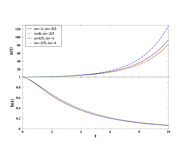
Figure 1: Time evolution of the scale factors $a(t)$ and $b(t)$ for $\Lambda_{6}>0$ and $k=0$.

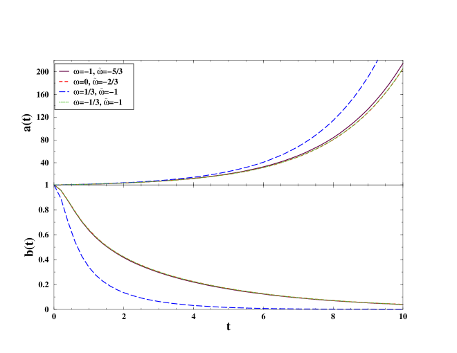
Figure 2: Time evolution of the scale factors $a(t)$ and $b(t)$ for $\Lambda_{6}>0$ and $k=-1$.

III-A. De Sitter Bulk

For $\Lambda_{6}>0$ we find that only negative values of $\hat{w}$ according to Table 1 give acceptable solutions for $k=0,-1$, while the $k=1$ solutions are not acceptable for any value of $\hat{w}$. A typical evolution of the two scale factors is shown in Fig. 1 and Fig. 2, for various values of $w$.

In both cases the scale factor $a(t)$ grows very fast, while the scale factor of the fourth dimension goes very fast to small values where it stays constant for the whole evolution. The reason for the fast growth of $a(t)$ is that the cosmological constant of the bulk $\Lambda_{6}$ acts as an effective cosmological constant on the brane and drives an exponential growth. This is common to the braneworld models with a cosmological constant in the bulk. It also happens in the five-dimensional Randall-Sundrum model if we do not impose the fine tuning between the brane tension and the five-dimensional cosmological constant.

III-B. Anti De Sitter Bulk

For $\Lambda_{6}<0$ and $k=0,1$ we do not get any acceptable solution. The scale factors either go to infinity, or $a(t)$ grows and $b(t)$ decays for a while and at some point they interchange behaviours, crossing each other and going to infinity. However, for $k=-1$ there is an interesting evolution of an oscillating universe shown in Fig. 3.

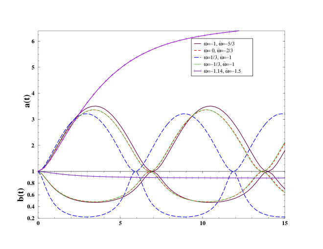
Figure 3: Time evolution of the scale factors $a(t)$ and $b(t)$ in an oscillating universe for $\Lambda_{6}<0$ and $k=-1$.

Again these solutions are obtained only for negative values of $\hat{w}$ according to Table 1 for various values of $w$. For $w<-1$ there is a small range of values near the critical value of $\hat{w}$, where $a(t)$ escapes from the oscillating behaviour and grows very fast, forcing $b(t)$ to decay and freeze out at certain small value analogously to De Sitter cases.

III-C. Minkowski Bulk

When $\Lambda_{6}$=0, we do not have the very strong effect of the bulk cosmological constant and the time evolution of the scale factors is smoother. If we had introduced a brane tension on the 4-brane, then a fine tuning similar to the Randall-Sundrum case in five-dimensions, would have resulted in the same behaviour. We show a typical time evolution of the two scale factors in Fig. 4, for $k=0,-1$ while there is no acceptable solution for $k=1$.

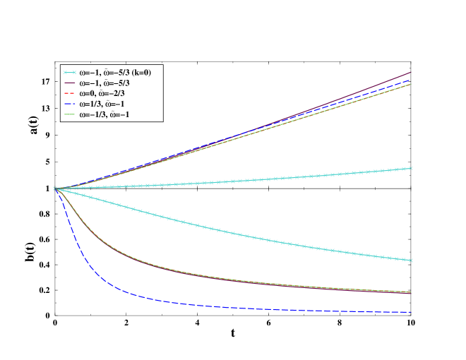
Figure 4: Time evolution of the scale factors $a(t)$ and $b(t)$ for $\Lambda_{6}=0$ and $k=0,-1$.

The evolution of the scale factor $a(t)$ is nearly linear for $k=-1$, while for $k=0$ there is an interesting solution with dark energy in the physical universe ($w=-1$) and with ”phantom” energy in the extra dimension ($\hat{w}=-5/3$). The $b(t)$ scale factor decays at a smaller rate compared with the case of a non-zero bulk cosmological constant, but soon it gets a small value where it freezes for the whole cosmological evolution. As it happens in all the other cases, $\hat{w}$ is negative in the range of values given in Table 1 for all acceptable solutions, indicating the need of dark energy to suppress the extra fourth dimension compared to the three other dimensions.

4. Conclusions

We presented a (4+1)-braneworld cosmological model in a six-dimensional bulk. If $a(t)=b(t)$, with $a(t)$ the usual scale factor of the three physical dimensions, and $b(t)$ the scale factor of the extra fourth dimension, we found the generalized Friedmann equation in six-dimensions of the Randall-Sundrum model describing the cosmological evolution of a four-dimensional brane-universe. We then showed that there is an equivalent description of a 4-brane moving in a static six-dimensional bulk and the cosmological evolution on the brane is described by the same generalized Friedmann equation.

If $a(t)\neq b(t)$ the four-dimensional universe evolves with two scale factors. However, for an observer in the moving brane, $a$ and $b$ are static depending only on the coordinate on which the 4-brane is moving. Then, demanding to have an effective Friedmann-like equation on the brane, we showed that the motion of the 4-brane in the static bulk is constrained by Darmois-Israel boundary conditions, resulting in a relation connecting $a$ and $b$ acting as a constraint of the brane motion.

The way $a$ and $b$ are related depends on the energy-matter content of the 4-brane, because their relation was derived from the consistency of the Darmois-Israel boundary conditions. We then explored what are the consequences of the presence of this constraint of motion for the cosmological evolution of the brane-universe. We assumed that the universe started higher-dimensional at the Planck scale with all the dimensions at the Planck length, and subsequently an anisotropy was developed between the three physical dimensions and the extra-dimension. We then followed the evolution by making a “phenomenological” analysis of how the two scale factors evolved under various physical assumptions. In all considered cases, (A)dS and Minkowski six-dimensional bulk, open, closed and flat brane-universe and matter, radiation, cosmological constant and dark energy dominated three-dimensional physical universe, we found that dark energy is needed for the dynamical suppression and subsequent freezing out of the extra fourth dimension.

It is interesting to further explore the relation we found between the cosmological evolution of a higher-dimensional brane-universe with the static properties of the bulk. The cosmological evolution on a higher-dimensional brane-universe is related to a topology change of the bulk during the evolution, and this relation might lead to a better understanding of the Gregory-Laflamme [22] instabilities of higher-dimensional objects.

References

- [1] D. N. Spergel et al. [WMAP Collaboration], Astrophys. J. Suppl. 148 (2003) 175 [arXiv:astro-ph/0302209].
- [2] R. Scranton et al. [SDSS Collaboration], [arXiv:astro-ph/0307335].
- [3] A. G. Riess, arXiv:astro-ph/9908237.
- [4] G. Goldhaber et al. [The Supernova Cosmology Project Collaboration], arXiv:astro-ph/0104382.
- [5] N. Arkani-Hamed, S. Dimopoulos and G. R. Dvali, Phys. Lett. B 429 (1998) 263 [arXiv:hep-ph/9803315], I. Antoniadis, N. Arkani-Hamed, S. Dimopoulos and G. R. Dvali, Phys. Lett. B 436 (1998) 257 [arXiv:hep-ph/9804398], N. Arkani-Hamed, S. Dimopoulos and G. R. Dvali, Phys. Rev. D 59 (1999) 086004 [arXiv:hep-ph/9807344].
- [6] L. Randall and R. Sundrum, Phys. Rev. Lett. 83, 3370 (1999) [arXiv:hep-ph/9905221], L. Randall and R. Sundrum, Phys. Rev. Lett. 83, 4690 (1999) [arXiv:hep-th/9906064].
- [7] R. Maartens, Living Rev. Rel. 7, 7 (2004) [arXiv:gr-qc/0312059].
- [8] E. Papantonopoulos, [arXiv:gr-qc/0410032], U. Gunther and A. Zhuk, [arXiv:gr-qc/0410130], D. Langlois, [arXiv:gr-qc/0410129].
- [9] P. Binetruy, C. Deffayet and D. Langlois, Nucl. Phys. B 565 (2000) 269 [arXiv:hep-th/9905012],
- [10] C. Csaki, M. Graesser, C. F. Kolda and J. Terning, Phys. Lett. B 462 (1999) 34 [arXiv:hep-ph/9906513], J. M. Cline, C. Grojean and G. Servant, Phys. Rev. Lett. 83 (1999) 4245 [arXiv:hep-ph/9906523], P. Kraus, JHEP 9912 (1999) 011 [arXiv:hep-th/9910149], A. Kehagias and E. Kiritsis, JHEP 9911 (1999) 022 [arXiv:hep-th/9910174], C. Csaki, M. Graesser, L. Randall and J. Terning, Phys. Rev. D 62 (2000) 045015 [arXiv:hep-ph/9911406], D. Ida, JHEP 0009 (2000) 014 [arXiv:gr-qc/9912002], C. Charmousis, Class. Quant. Grav. 19, 83 (2002) [arXiv:hep-th/0107126].
- [11] R. H. Brandenberger and C. Vafa, Nucl. Phys. B 316, 391 (1989).
- [12] S. Alexander, R. H. Brandenberger and D. Easson, Phys. Rev. D 62, 103509 (2000) [arXiv:hep-th/0005212].
- [13] P. Kanti, R. Madden and K. A. Olive, Phys. Rev. D 64, 044021 (2001) [arXiv:hep-th/0104177].
- [14] N. Arkani-Hamed, S. Dimopoulos, N. Kaloper and J. March-Russell, Nucl. Phys. B 567, 189 (2000) [arXiv:hep-ph/9903224].
- [15] P. Binetruy, C. Deffayet, U. Ellwanger and D. Langlois, Phys. Lett. B 477 (2000) 285 [arXiv:hep-th/9910219],
- [16] C. Csaki, J. Erlich and C. Grojean, Nucl. Phys. B 604, 312 (2001) [arXiv:hep-th/0012143]. P. Bowcock, C. Charmousis and R. Gregory, Class. Quant. Grav. 17, 4745 (2000) [arXiv:hep-th/0007177],
- [17] T. Shiromizu, K. i. Maeda and M. Sasaki, Phys. Rev. D 62, 024012 (2000) [arXiv:gr-qc/9910076]. S. Mukohyama, Phys. Lett. B 473, 241 (2000) [arXiv:hep-th/9911165]. R. Maartens, Phys. Rev. D 62 (2000) 084023 [arXiv:hep-th/0004166],
- [18] E. Abdalla, A. Casali and B. Cuadros-Melgar, Nucl. Phys. B 644, 201 (2002) [arXiv:hep-th/0205203].
- [19] B. Cuadros-Melgar, ”Gravitational Shortcuts in Brane Cosmology”, PhD Thesis, Examined June 2003, Universidade de São Paulo, Brazil.
- [20] B. Cuadros-Melgar, Class. Quant. Grav. 21, 2669 (2004) [arXiv:hep-th/0303131].
- [21] S. Mukohyama, T. Shiromizu and K. i. Maeda, Phys. Rev. D 62, 024028 (2000) [Erratum-ibid. D 63, 029901 (2001)] [arXiv:hep-th/9912287].
- [22] R. Gregory and R. Laflamme, Phys. Rev. Lett. 70 (1993) 2837 [arXiv:hep-th/9301052].