Decay of the Cosmological Constant. Equivalence of Quantum Tunneling and Thermal Activation in Two Spacetime Dimensions

Abstract

We study the decay of the cosmological constant in two spacetime dimensions through production of pairs. We show that the same nucleation process looks as quantum mechanical tunneling (instanton) to one Killing observer and as thermal activation (thermalon) to another. Thus, we find another striking example of the deep interplay between gravity, thermodynamics and quantum mechanics which becomes apparent in presence of horizons.

I Introduction and Summary

The need to reconcile the observed small value of the cosmological constant with the value that standard elementary particle theory predicts is a major challenge of theoretical physics Weinbergetal . A number of years ago, a possible mechanism for relaxing $\Lambda$ was proposed BT . Its essential aspect is the nucleation of membranes (domain walls). The cosmological constant, which becomes a dynamical field, jumps across the membrane and it is decreased inside it. In the version of the mechanism proposed in BT , the membranes were nucleated through quantum-mechanical tunneling, for which the path integral is dominated by an instanton solution of the Euclidean equations of motion. Recently GHTW , a novel variant of this mechanism has been proposed in which the membranes are created through classical thermal effects of de Sitter space rather than quantum-mechanically (see Garriga ; Hackworth for related recent discussions). The Euclidean solutions relevant to this process were named “thermalons”. These new solutions are time-independent in contradistinction with the instantons, which are time-dependent.

In order to obtain additional insight into the thermalons, we shall examine their analog in the simple possible context of two-dimensional spacetime. In doing so we encounter yet another fascinating instance of the subtle interplay between gravity, thermodynamics and quantum theory, which becomes apparent in the presence of event horizons. The most famous instance of this interplay is, of course, the Bekenstein-Hawking formula for black hole temperature and entropy.

In brief, what we found is the following: If one describes the process in terms of the so-called global coordinates for de Sitter space, in which the volume of the spatial sections is proportional to the hyperbolic cosine of time, the nucleation of membranes occurs through the exact analog of the ($3+1$)-dimensional instanton, as it was already noted in BT . On the other hand, if one describes the process in terms of the static coordinates for de Sitter space, the membranes are nucleated through the thermalon, that is a classical thermodynamical effect. It is to be emphasized that when we say “… describes in terms of coordinates …”, we are talking about just a change of coordinates in one and the same spacetime : two portions of de Sitter spaces of different radii of curvature joined across the membrane.

Thus, one and the same physical process appears in one description as a strictly quantum-mechanical tunneling effect and, in the other, as a classical metastability effect (going over the barrier rather than tunneling through it). There is no paradox here because one may say that when the coordinates are changed, the “potential” is also changed so the barrier that one tunnels through in one case is not the same barrier over whose top one goes in the other. It is also quite alright that the thermodynamic description should appear when the static coordinates are used, since it would appear natural to think that time-independence amounts to equilibrium.

II Instantons and thermalons

To make the discussion self-contained we briefly review here the concept of “thermalon”. We also compare and confront it with the concept of instanton. Consider a non-relativistic one-dimensional particle placed in a potential $V(r)$, as shown in Fig. 1. The particle is initially in a metastable minimum (the “false vacuum”), at $x=0$. The particle may decay to the “true vacuum” at $x=x_{t}$ by two different mechanisms: It can either (i) tunnel through the potential barrier or (ii) it can go over the barrier by a thermal kick.

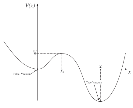
Figure 1: A particle in a potential is initially in a metastable state at $x=0$ (false vacuum). It may end up in the true vacuum at $x=x_{t}$ either by tunneling through the potential barrier or by a thermal kick.

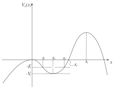
Figure 2: The Euclidean system consists in the particle placed in a potential $V_{E}=-V$. The Euclidean path integral is evaluated in the semiclassical limit. At zero temperature, the solution that dominates the path integral is the instanton which starts at rest at $x=0$, $t=-\infty$, bounces at $x=x_{b}$ and comes back to $x=0$ at $t=\infty$. At higher inverse temperatures $\beta$, the corresponding instantons are periodic orbits, bounded between two turning points, $x_{1}$, $x_{2}$, with period $\beta\hbar$. This happens at some particular value of the energy $-E$. When the temperature is high enough the static orbit at the bottom of the potential well $x=x_{0}$, the thermalon, becomes dominant.

For the tunneling problem, if one were to treat the problem exactly one would start with a wave packet localized around $x=0$ and calculate the quantum mechanical amplitude to propagate from $x=0$ to $x=x_{t}$. This one could do in principle at any arbitrary inverse temperature $\beta$ by computing the path integral. In the semiclassical approximation the path integral is dominated by a solution of the classical equations of motion in imaginary time (“Wick rotation”, “Euclidean continuation”). The calculation is further simplified at zero or very low temperatures $\beta^{-1}$.

For the thermal excitation the solution is again given by an Euclidean path integral (the partition function), which now is most simply dealt with for $\beta^{-1}$ large enough to go over the top of the barrier by a “thermal kick”. For tunneling, the classical solution is called the instanton and it is described in Fig. 2. The particle starts at rest from the false vacuum at $t=-\infty$, bounces at $x=x_{b}$ and comes back to the false vacuum at $t=\infty$. The decay rate takes the form coleman ; affleck

$$\Gamma=\frac{2}{\hbar}\mbox{Im}F\ \ \ \ \ \ \ \ \ \mbox{(quantum tunneling)}.$$ (1)

For a thermal kick the classical solution is called a thermalon. The particle sits at all times at the stable equilibrium position $x=x_{0}$ of the Euclidean potential of Fig. 2. The decay takes the form langer ; affleck

$$\Gamma=\frac{\omega\beta}{\pi}\mbox{Im}F\ \ \ \ \ \ \mbox{(thermal activation)}.$$ (2)

In both Eq. (1) and Eq. (2), $F$ is the Helmholtz free energy given by

$$\beta F=\beta U-S,$$ (3)

where $U$ is the internal energy and $S$ the entropy. In Eq. (2), $\omega$ is the frequency of oscillations in Euclidean time around $x=x_{0}$ (Fig.(2)),

$$\omega=V^{\prime\prime}_{E}(x_{0}).$$ (4)

If one evaluates the path integral to imaginary time,i.e.

$$x(t)=x_{E}(it_{E}),\ \ \ \ \ \ iI[x(t)]=I(x_{E}(t_{E})),$$ (5)

one has

$$\int{\cal D}x_{E}e^{\frac{i}{\hbar}I_{E}}=e^{-\beta F},$$ (6)

where “$E$” stands for “Euclidean” and the functional integral is evaluated over closed paths $x_{E}(t_{E})$ with Euclidean time period

$$\Delta t_{E}=\hbar\beta.$$ (7)

For tunneling as well as for thermal activation, the semiclassical rates take the form,

$$\Gamma=Ae^{-B},$$ (8)

where $B$ is the classical Euclidean action divided by $\hbar$ and $A$ is a prefactor which involves the determinant of a differential operator coleman , and which will not be discussed here.

The properties of instantons and thermalons are illustrated and discussed in Fig.2 and summarized in Table I affleck ; linde .

Table 1: Instantons and Thermalons Compared and Contrasted.

Solution of the classical Equation of motion	Process that the solution describes when used to dominate path integral	Dependence on Euclidean time for motion in one-dimensional      potential	Range of validity if used to approximate decay rate by steepest descent	Formula for decay rate
Instanton at zero temperature	Tunneling through potential barrier	Time dependent. Starts at $x_{1}$ at $t=-\infty$, bounces at $x_{2}$ and comes back to $x_{1}$ at $t=\infty$. The bounce is localized in time.	Zero temperature	Γ=2ℏImF=2ℏImE
Instanton at non-zero temperature	Tunneling through potential barrier at non-zero temperature	Time dependent, starts at $x_{1}$, bounces at $x_{2}$ and comes back to $x_{1}$ after a full period $\Delta t=\beta$.	Dominates for 2πω≪βℏ¡∞	Γ=2ℏImF
Thermalon	Going over the barrier by a thermal kick	Time independent.    Stands at the bottom of the Euclidean potential for all times.	Dominates for 0¡βℏ≪2πω	Γ= ωβπImF
			In overlap region, $\beta\hbar\sim\frac{2\pi}{\omega}$, both solutions should in general be included. Here $\omega$ is the frequency of oscillations in Euclidean time of perturbations around the thermalon. It is assumed that there is only one such stable Euclidean mode. For motion in a potential, $\omega=V^{\prime\prime}(x_{T})$.	$F$ has imaginary part because the extremum is a saddle point due to unstable state.

III Pair creation in flat spacetime

III.1 Instanton

In two spacetime dimensions, a closed membrane, which may be thought of as the boundary of a ball, becomes a pair of points, which are the boundary of an interval. Thus, we will be considering pair creation. The term “pair creation” is all the more appropriate since the analog of the $3$-form potential appearing in four spacetime dimensions is, in two spacetime dimensions, just the ordinary electromagnetic potential. Therefore, our problem is pair creation by an electric field coupled to gravity. The action will be taken to be the sum of four terms: (i) The length of the worldline times the mass of the particle, (ii) the minimal coupling to the electromagnetic field, (iii) the Maxwell action, (iv) the gravitational action, for which we will use the functional proposed in CT . However, for the sake of focusing as clearly as possible on the central point, we shall start by considering pair creation in flat spacetime in a constant external electric field $E$. This is of interest because even this simplified process accepts the two alternative interpretations, namely, quantum mechanical or thermodynamical depending on the coordinate system we choose in our description.

The Euclidean action, describing a particle of charge $q$ and mass $m$, with worldline parameterized by $z^{\mu}(\lambda)$, in an external electromagnetic field $A_{\mu}=(Ex,0)$ is

$$I=m\int\sqrt{\dot{z}^{\mu}\dot{z}_{\mu}}d\tau-q\int A\ =m(\mbox{length})-qE(\mbox{area}).$$ (9)

The overall sign of the action has been chosen so that one path integrates $e^{-I}$.

In Cartesian coordinates, the action (9) reads

$$I=\int d\lambda\left[m\sqrt{\dot{t}^{2}+\dot{x}^{2}}-qEx\dot{t}\right],$$ (10)

where $\lambda$ is a parameter that increases along the worldline. The momentum $P_{t}$ conjugate to $t$ is given by

$$P_{t}=m\frac{\dot{t}}{\sqrt{\dot{t}^{2}+\dot{x}^{2}}}-qEx=\mbox{sgn}(\dot{t})\frac{m}{\sqrt{1+\left(\frac{dx}{dt}\right)^{2}}}-qEx.$$ (11)

The instanton solution is a complete circle in the $(x,t)$–plane centered at $(t_{0},x_{0})$ with radius $R$ equals to

$$R=m/qE,$$ (12)

where $t_{0}$ and $x_{0}$ are integration constants (See Fig 3). One may describe it as follows. The system is initially in the metastable vacuum (no particle). At $t_{0}-R$, a particle-antiparticle pair appears. The particles then propagate and annihilate at $t_{0}+R$, leaving back the metastable vacuum.

Note that this is the most general solution of the equations of motion. This is an instanton at zero temperature, because it is time dependent and localized in time (see Table I). The instanton remains a solution if one identifies Euclidean time with a period $\hbar\beta$ provided the circle of Fig. 3 fits into the corresponding cylinder, i.e.,

$$2R<\hbar\beta.$$ (13)

It is then an instanton at non-zero temperature $\beta^{-1}$.

The action evaluated on this orbit is

$$I_{0}=\frac{\pi m^{2}}{qE}\ ,$$ (14)

which is the Schwingerschwinger result for two–dimensional spacetime.

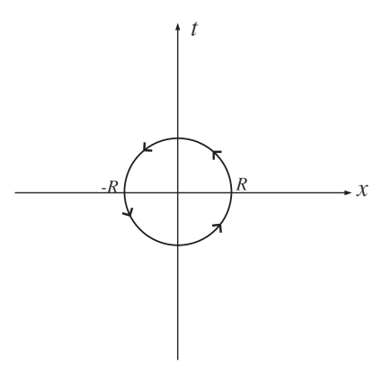
Figure 3: The instanton is an oriented circle of radius $R=m/qE$ centered at any point $(t_{0},x_{0})$ of the Euclidean plane.

The tunneling decay rate described by the instanton is, in the semiclassical approximation,

$$\Gamma\sim e^{-I_{0}/\hbar}=e^{-\frac{m^{2}\pi}{qE}}\ .$$ (15)

III.2 Thermalon

The above interpretation changes radically if we use polar coordinates,

$$t = r\sin(\tau/L)$$ (16)

$$x = r\cos(\tau/L)\ .$$ (17)

Here $L$ is some arbitrary length scale. In the Lorentzian continuation, these are Rindler coordinates adapted to an observer of proper acceleration $1/L$. The metric takes the form

$$ds^{2}=\frac{r^{2}}{L^{2}}d\tau^{2}+dr^{2}\ ,$$ (18)

The acceleration of a stationary particle at $r$ is $1/r$. The observer located at $r=L$ has the special property that on his trajectory the Killing vector $d/d\tau$ has unit norm.

The Euclidean Rindler “time” coordinate $\tau$ has a periodicity $2\pi L$ and is identified with the inverse Unruh temperature seen by the associated Lorentzian accelerated observer at $r=L$,

$$\beta=\frac{2\pi L}{\hbar}\ .$$ (19)

The action (9) now reads,

$$I=\int d\lambda\left[m\sqrt{\dot{r}^{2}+\frac{r^{2}}{L^{2}}\dot{\tau}^{2}}-\frac{qE}{2L}r^{2}\dot{\tau}\right].$$ (20)

We evaluate the conserved momentum $P_{\tau}$ conjugate to $\tau$,

$$P_{\tau}=\frac{m\dot{\tau}}{\sqrt{\frac{L^{2}}{r^{2}}\dot{r}^{2}+1}}-\frac{Eqr^{2}}{2L}=\frac{m\ \mbox{sgn}(\dot{\tau})}{\sqrt{\frac{L^{2}}{r^{2}}\left(\frac{dr}{d\tau}\right)^{2}+1}}-\frac{Eqr^{2}}{2L}.$$ (21)

Contrary to what happens in Cartesian coordinates, the dynamical system admits now static solutions. In fact, there is only one such solution, given by

$$r=R=\frac{m}{Eq},$$ (22)

and

$$P_{\tau}=\frac{1}{2}\frac{m^{2}}{LEq}=\frac{1}{2}m\left(\frac{R}{L}\right).$$ (23)

Because it is static and stable (see below), this solution is a thermalon. The value of $R$ given by (22) is, of course, just Eq. (12). This was expected, and it is the main point that we are making, namely, that the instanton as seen in a polar system of coordinates, centered a the origin $t_{0}=x_{0}=0$, is the thermalon.

A small perturbation of the solution amounts to translating the center of the circle. When viewed in Rindler coordinates, this appears as a periodic motion with same period as $\tau$. So, the solution is stable and the frequency of oscillations around the thermalon is,

$$\omega_{\tau}=\frac{1}{L}\ .$$ (24)

The thermalon describes the probability for the particle to jump over the potential barrier by a thermal fluctuation. The thermal decay rate is given by Eq. (8), which, in the thermalon case, reduces to the Boltzmann factor,

$$\Gamma\sim e^{-\beta{\cal E}}\ ,$$ (25)

where the energy ${\cal E}$ is the conserved momentum $P_{\tau}$, and $\beta$ the corresponding inverse Unruh temperature. Explicitly, one gets,

$$\beta{\cal E}=\frac{2\pi L}{\hbar}\frac{1}{2}\frac{m^{2}}{LEq}=\frac{\pi m^{2}}{qE\hbar}.$$ (26)

Note that although $\beta$ and ${\cal E}$ depend on $L$, this length scale drops out from the product $\beta{\cal E}$. The value of $\beta{\cal E}$ given by Eq. (26) is exactly the value of the action (14) for the instanton. What underlies these “coincidences” is, of course, that the thermalon is just the instanton described in a different coordinate system. However, we are not facing a triviality, because the concepts associated to each description are drastically different. In the instanton framework, we are analyzing a quantum mechanical process at zero temperature, while in the thermalon description, we are working out a classical thermodynamical instability at non-zero temperature. Thus, we have in a very simple context, an example of the inextricable connection between gravity, quantum mechanics and thermodynamics, which was first observed in the context of black hole entropy.

The equivalence of the two representations does not just happen for the exponent in the transition rate, but in fact for the complete decay rates. Indeed, if we multiply the temperature (19) and the frequency (4) and divide the product by $\pi$ to evaluate the multiplicative factor characteristic of the metastability calculation, Eq. (2), we find

$$\frac{\omega_{\tau}\beta}{\pi}=\frac{1}{L}\frac{2\pi L}{\hbar}\frac{1}{\pi}=\frac{2}{\hbar}\ ,$$ (27)

which is exactly the corresponding tunneling expression, Eq. (1).

Eq. (27) tells us that we are precisely in the overlap region where both the thermalon and the instanton should be considered when computing the free energy $F$ (see table I). However, in this example there is only one Euclidean solution. It is just that it is interpreted differently in different coordinate systems. This unique solution is the one that dominates the path integral in the present case.

As a final comment, we recall that in $D$ spacetime dimensions, the symmetry group of the instanton at zero temperature is $SO(D)$, while the symmetry group of the thermalon is $SO(D-1)\times SO(2)$. For the special case of two dimensions the two groups coincide, in agreement with the fact that the instanton and the thermalon are one and the same solution.

IV Coupling to gravity

The complementary description of one and the same physical process (pair creation) as a quantum mechanical effect or as a thermal effect is also available when we switch on gravity. The actual calculations describing pair creation in a gravitational field have already been done in BT . As it was stated in the introduction, the main novelty of the present work is the complementary interpretation of the process as a thermal effect.

We will first remind the reader of the results of BT in the two–dimensional case and introduce some notation. The equation of motion to be used for the gravitational field is CT

$$\frac{1}{2}R-\lambda=\kappa T\ \ ,$$ (28)

where $T$ is the trace of the energy-momentum tensor, and $\kappa$ a positive coupling (which would equal $8\pi G$ in four dimensions). In our case, the energy momentum is the one produced by an electromagnetic field $F_{\mu\mu}$ and a particle of mass $m$ and charge $q$. The Maxwell equations for the electromagnetic field imply that $F_{\mu\nu}=\sqrt{g}E\epsilon_{\mu\nu}$, where $\epsilon_{\mu\nu}$ is the Levi-Civita symbol in two dimensions and $E$ is a constant in the absence of sources. The value of $E$ jumps when crossing the worldline of the particle, so that,

$$E_{+}-E_{-}=q\ .$$ (29)

We will adopt the convention that, when traveling along the worldline of the particle, the “interior” (”-” region) will be on the right hand side. The ”+” region will be called the ”exterior”. For the gravitational field, the electromagnetic field will contribute to an effective cosmological constant,

$$\Lambda_{\pm}\equiv\frac{1}{l_{\pm}^{2}}=\lambda+\kappa E_{\pm}^{2}\ .$$ (30)

Therefore, at each side of the worldline, the geometry will be that of a two–sphere of radii $l_{+}$ and $l_{-}$ respectively,

$$ds^{2}_{\pm}=l^{2}_{\pm}(d\theta^{2}+\sin^{2}\theta_{\pm}d\phi_{\pm}^{2})\ \ \ \ (0\leq\theta_{\pm}\leq\pi,\ 0\leq\phi_{\pm}\leq 2\pi)\ .$$ (31)

By taking the range of $\phi$ to go from $0$ to $2\pi$, we are excluding conical singularities at the poles. Note that we may always rotate the coordinate systems on each of the glued spheres so that when embedded in flat three-dimensional space their corresponding $z$–axis coincide. This means that we can set $\phi_{+}=\phi_{-}\equiv\phi$. The worldline of the particle is determined by the matching conditions obtained by integrating (28) across the membrane. One gets

$$K_{+}-K_{-}=\kappa m\ ,$$ (32)

where $K_{\pm}$ are the extrinsic curvatures of the worldline as embedded in each sphere (see for example BT ).

We now define

$$\rho_{\pm}=l_{\pm}\sin\theta_{\pm}.$$ (33)

and parameterize the curve using the arclength $s$, so that the extrinsic curvature is given by

$$K_{\pm}=\frac{1}{\rho_{\pm}\dot{\rho}_{\pm}}\left(1-\frac{\rho^{2}_{\pm}}{l^{2}_{\pm}}\right)^{1/2}\frac{d}{d\tau}\left(\rho_{\pm}^{2}\dot{\phi}_{\pm}\right)\ .$$ (34)

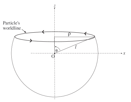
Figure 4: Each de-Sitter two-sphere is parameterized as shown in the figure. The angle $\phi$ runs anti–clockwise around $z$. Instead of $\theta$ we may also use the coordinates $\rho=l\sin\theta$. In this case, however, the parameterization will cover only half of the sphere. A solution for the worldline of the particle has been drawn, and the “exterior” region has been removed.

The trajectory is a circle which we take at some constant $\rho_{\pm}$ (see Fig. 4). From Eqs. (32) and (34) we get,

$$\epsilon_{+}\sqrt{\frac{1}{\rho_{+}^{2}}-\frac{1}{l_{+}^{2}}}-\epsilon_{-}\sqrt{\frac{1}{\rho_{-}^{2}}-\frac{1}{l_{-}^{2}}}=km,$$ (35)

where $\epsilon_{\pm}=\mbox{sgn}(\dot{\phi}_{\pm})$. Because the length of the circle must be the same as seen from each side, we must take $\rho_{-}=\rho_{+}\equiv\bar{\rho}$ on the orbit. Eq. (35) yields then

$$\bar{\rho}^{2}=\frac{l_{+}^{2}}{1+\gamma^{2}}\ ,$$ (36)

where

$$\alpha^{2}=\frac{1}{l_{+}^{2}}-\frac{1}{l_{-}^{2}}=2\kappa qE_{av}\ ,$$ (37)

$$E_{av}=\frac{1}{2}\left(E_{+}+E_{-}\right)\ ,$$ (38)

and

$$\gamma=\frac{l_{+}(\alpha^{2}-\kappa^{2}m^{2})}{2m\kappa}.$$ (39)

Therefore, the classical Euclidean solution, the exponential of whose action appears in the probability, consists of two two-dimensional spheres of radii $l_{+}$ and $l_{-}$ joined at a circle of radius $\bar{\rho}$.

IV.1 Instanton

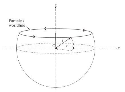
Figure 5: Instanton interpretation. In each region we choose spherical coordinates such the azimuthal angle $\chi$ is measured from the $x$ axis. The angle $\xi_{\pm}$ goes anti-clockwise around the $x$ axis. In the radial coordinate $r=l\cos\chi$ the metric takes the Schwarzschild-de Sitter form of Eq. (42). The trajectory of the particle $r(t)$ is time-dependent in the Euclidean time $t=l\xi$.

We can choose different coordinate systems to describe the above solution. The interpretation of the solution will depend on this choice. The instanton picture is obtained by choosing spherical coordinates as in Fig. 5, i.e.,

$$ds^{2}_{\pm}=l^{2}_{\pm}(d\chi_{\pm}^{2}+\sin^{2}\chi_{\pm}d\xi_{\pm}^{2})\ \ \ \ (0\leq\chi_{\pm}\leq\pi,\ 0\leq\xi_{\pm}\leq 2\pi).$$ (40)

The angle $\chi_{\pm}$ is now measured from the $x$ axis, and $\xi_{\pm}$ goes anti-clockwise around the $x$ axis. The Euclidean time is $t_{\pm}=l_{\pm}\xi_{\pm}$. The worldline of the particle is time-dependent and turns out to be exactly the instanton solution discussed in BT .

To describe it more explicitly, define $r_{\pm}=l_{\pm}\cos\chi_{\pm}$. Again, the coordinates $r_{+}$ and $r_{-}$ must be related on the worldline of the particle so that the total length is the same as seen from each side. The relation may be obtained by noting that in terms of the previous coordinate system,

$$r_{\pm}=\rho_{\pm}\sin\phi,$$ (41)

Now, we know that $\rho_{+}=\rho_{-}$ on the trajectory, and therefore, we have that $r_{+}=r_{-}\equiv r$. The metric takes the Schwarzschild-de Sitter form

$$ds^{2}_{\pm}=f^{2}_{\pm}dt^{2}_{\pm}+f_{\pm}^{-2}dr^{2},$$ (42)

with

$$f^{2}_{\pm}=1-\frac{r^{2}}{l_{\pm}^{2}},$$ (43)

and the trajectory, as seen from each side, is given by

$$r(t)=\pm l\sqrt{\left(1-\frac{\cos^{2}\theta_{0}}{\cos^{2}{(t/l)}}\right)},\ \ \ \ \ \ \theta_{0}\leq t/l\leq\theta_{0},$$ (44)

where, for the sake of clarity, the subscripts $\pm$ have been dropped. The angle $\theta_{0}$ is a constant, which, for each region, is given by Eqs. (33) and (36). As for the instanton in flat space, there are two points on the trajectory for each value of $t$. Furthermore, if we take the limit $\kappa\rightarrow 0$ we end up with the instanton in flat spacetime of Sec. IIIA. To see this one has to recall that the bare cosmological constant, $\lambda$, coming from “the rest of physics” in Eq. (28) is of the form

$$\lambda=\kappa\rho_{vac},$$ (45)

where $\rho_{vac}$ is the energy density of the vacuum. When we take the limit, the cosmological constant $1/l^{2}_{\pm}$ goes to zero in both regions,

$$\frac{1}{l_{\pm}}=\kappa\left(\rho_{vac}+E_{\pm}^{2}\right),$$ (46)

and therefore the metrics in Eq. (42) become flat Minkowski line elements in polar coordinates. Furthermore, the radius of the orbit, given by Eq. (36), goes into

$$\bar{\rho}^{2}=\frac{l_{+}^{2}}{1+\gamma^{2}}\stackrel{{\scriptstyle\kappa\rightarrow 0}}{{\longrightarrow}}\frac{1}{\frac{1}{l_{+}^{2}}+\frac{(E_{+}^{2}-E_{-}^{2})^{2}}{4m^{2}}}\stackrel{{\scriptstyle\kappa\rightarrow 0}}{{\longrightarrow}}\frac{m^{2}}{q^{2}E_{av}^{2}}\ ,$$ (47)

This is exactly the radius we obtained in the flat space case in Eq.(12).

IV.2 Thermalon

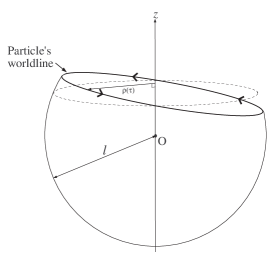
Figure 6: The diagram depicts a small perturbation on the thermalon alignment of Fig. 4. The radius $\rho(\tau)$ oscillates with a period equal to $2\pi l$, the total period of the time coordinate $t$.

The thermalon picture is obtained by analyzing the trajectory in the original coordinate system of Fig. 4. The solution is then clearly static. The metric takes the form

$$ds^{2}_{\pm}=\frac{d\rho^{2}}{1-\frac{\rho^{2}}{l^{2}_{\pm}}}+\frac{\rho^{2}}{l^{2}_{\pm}}dt_{\pm}^{2}\ ,$$ (48)

with the “Euclidean time” $t_{\pm}=l_{\pm}\phi$. It is interest to see at this point how one may recover the flat space background analysis of the previous section as a limiting case of the present discussion. Taking the limit $\kappa\rightarrow 0$ we must define a new, rescaled time coordinate $\tau$,

$$t_{\pm}=\frac{l_{\pm}}{L}\tau,$$ (49)

with $L$ being an arbitrary constant with dimension of length. In the limit, we get flat spacetime in polar coordinates as in Eq. (18).

In the coordinate system used in Fig. 4, the particle remains at a fixed value of $\rho$ at all times. However, if we rotate the worldline of the particle as in Fig. 5, the new solution will not be static in this set of coordinates. The curves ($\rho_{+}(\tau),t_{+}(\tau)$) and ($\rho_{-}(\tau),t_{-}(\tau)$) as seen from each side of the particle’s trajectory will oscillate around the static solution with frequency

$$\omega_{\pm}=1/l_{\pm},$$ (50)

since, in the absence of a conical singularity, the period of the time coordinate in (48) must be $2\pi l_{\pm}$. Therefore, the solution has the two key properties of a thermalon: Is a static and stable Euclidean solution of the theory.

We now may identify the temperature felt by an observer at each region with the respective de–Sitter temperature,

$$T_{\pm}=\frac{1}{\beta_{\pm}}=\frac{\hbar}{2\pi l_{\pm}}$$ (51)

and immediately note that,

$$\frac{\omega_{\pm}\beta_{\pm}}{\pi}\frac{1}{l_{\pm}}\frac{2\pi l_{\pm}}{\hbar}\frac{1}{\pi}=\frac{2}{\hbar}\ .$$ (52)

We see that, again, the two expressions for the probability (1) and (2) coincide.

To obtain an expression for the decay rate, we need to compute Im$F$ in expression (1) or (2), which, in our case are equivalent. This has been done before for the instanton, and, as have shown in the present work, both the instanton and the thermalon are one and the same process in two dimensions. For the sake of completeness we will quote here the known expressions. The result is of the form (8). The value of the action $B$ was computed in BT and takes the value,

$$I=4\pi\bar{\rho}m-\frac{2\pi}{\kappa}\log\left(1+\frac{\kappa ml_{+}}{(\sqrt{1+\gamma^{2}}-\gamma)(1-\alpha^{2}l_{+}^{2})}-\alpha^{2}l_{+}^{2}\right),$$ (53)

with $\alpha^{2}$, $\gamma$ defined in (37) and (39) respectively.

- (1) S. Weinberg, Rev. Mod. Phys. 61, 1 (1989);
- (2) J. D. Brown and C. Teitelboim, Nucl. Phys. B 297, 787 (1988).
- (3) A. Gomberoff, M. Henneaux, C. Teitelboim and F. Wilczek, Phys. Rev. D 69, 083520 (2004) [arXiv:hep-th/0311011].
- (4) J. Garriga and A. Megevand, Int. J. Theor. Phys. 43, 883 (2004) [arXiv:hep-th/0404097].
- (5) J. C. Hackworth and E. J. Weinberg, “Oscillating bounce solutions and vacuum tunneling in de Sitter spacetime,” arXiv:hep-th/0410142.
- (6) S. R. Coleman, Phys. Rev. D 15, 2929 (1977) [Erratum-ibid. D 16, 1248 (1977)].
- (7) I. Affleck, Phys. Rev. Lett. 46, 388 (1981).
- (8) J. S. Langer, Annals Phys. 54, 258 (1969).
- (9) A. D. Linde, Phys. Lett. B 70, 306 (1977); Phys. Lett. B 100, 37 (1981); Nucl. Phys. B 216, 421 (1983) [Erratum-ibid. B 223, 544 (1983)];
- (10) C. Teitelboim, Phys. Lett. B 126, 46 (1983); Phys. Lett. B 126, 41 (1983); “The Hamiltonian Structure Of Two-Dimensional Space-Time And Its Relation With The Conformal Anomaly,” in Quantum Theory of Gravity, S. Christensen (Editor), (Adam Hilger, Bristol, 1984).
- (11) J. S. Schwinger, Phys. Rev. 82, 664 (1951).