Coleman meets Schwinger!

Abstract

It is well known that spherical D–branes are nucleated in the presence of an external RR electric field. Using the description of D–branes as solitons of the tachyon field on non–BPS D–branes, we show that the brane nucleation process can be seen as the decay of the tachyon false vacuum. This process can describe the decay of flux–branes in string theory or the decay of quintessence potentials arising in flux compactifications.

One of the most beautiful results in Quantum Field Theory, derived by Schwinger Schwinger , is that pairs of charged particles are produced in an external electric field. This mechanism can be generalized to the nucleation of spherical branes in theories with $p$–form gauge potentials and was studied in Teitelboim using semiclassical instanton methods, starting from the Nambu–Goto brane action minimally coupled to the gauge field. String theory has many extended charged objects associated to massless gauge fields and therefore analogous computations of brane nucleation rates can be performed.

According to Sen Senrev , D–branes can be thought of as tachyon solitons. It is therefore natural to ask if the brane nucleation process can be described in this language. Consider, in particular, the tachyon kink solution on a non–BPS D$p$–brane that interpolates between the $T=\pm\infty$ vacua of the tachyon field and which describes a BPS D$(p-1)$–brane. By turning on an external RR electric field

$$dC_{p}=E\,\,dt\wedge dx^{1}\wedge\cdots\wedge dx^{p}$$

parallel to the worldvolume of a non–BPS D$p$–brane, we shall see that the tachyon vacuum degeneracy is lifted and that the brane nucleation corresponds to the decay of the tachyon false vacuum. Hence Coleman’s analysis of the decay of the false vacuum Coleman describes Schwinger’s nucleation process. Similar methods were used in Hashimoto to describe brane/anti–brane decay by creation of a throat throat .

We shall take as closed string background for our computations flat space with a small RR electric field and we shall neglect the backreaction on the closed string geometry. The electric field $E$ will in general distort the geometry on length scales larger than $1/E$, therefore our analysis will be valid only within this scale. There are two simple settings to keep in mind. Firstly, whenever the directions transverse to the electric field are not compact, the background geometry is that of a flux–brane fluxbranes . The electric field self–gravitates on the length scale $1/E$ and the non–BPS brane is placed at the center of the flux–brane, which is a gravitationally stable point. In this language the decay of the flux–brane towards flat space is explicitly described as the decay of the open string false vacuum of many non–BPS D-branes. Secondly, whenever the transverse directions are compact, the electric field will give rise to a quintessence potential in the compactified theory CCK . The decay of the tachyon field will then describe the decay of the quintessence potential. This process generalizes the dynamical decay of the cosmological constant of BrownTeit . We shall neglect the effect of the expansion of the universe in the tachyon dynamics.

Throughout this paper we neglect closed string effects by taking $\alpha^{\prime}E^{2}\ll 1$ and $g_{s}\ll 1$. Therefore we can consider the open string dynamics independently, ignoring the backreaction on the closed string fields. The effects in the closed string fields due to the vacuum decay can be computed to leading order and describe a change of order $g_{s}$. We work in units such that $\alpha^{\prime}=1$.

Recall the form of the classical action for the tachyon field on a non–BPS D$p$–brane Senrev

$$S = -\int d^{p+1}x\,V(T)\sqrt{1+\eta^{\mu\nu}\partial_{\mu}T\partial_{\nu}T}$$ (1)

$$+\int W(T)\,dT\wedge C_{p}\ ,$$

where the massless fields on the brane are consistently set to zero and $\mu,\nu=0,1,\cdots,p$. We consider flat space–time with a constant dilaton, but we allow for the presence of a RR $p$–form potential. Several properties of the functions $V(T)$ and $W(T)$ are known. Both are even functions and behave asymptotically as $e^{-|T|/\sqrt{2}}$. Moreover, $V(0)=\tilde{T}_{p}$ is the tension of the non–BPS D$p$–brane, which is related to the tension $T_{p}$ of a BPS D$p$–brane by $\tilde{T_{p}}=\sqrt{2}\,T_{p}$. Finally, the fact that the tachyon kink solution represents a BPS D$(p-1)$–brane gives the additional requirements

$$\int_{-\infty}^{\infty}dT\,V(T)=\int_{-\infty}^{\infty}dT\,W(T)=T_{p-1}\ ,$$

so that the tension and charge of the soliton are correctly normalized. The qualitative results in this note will not depend on the specific form of the functions $V(T)$ and $W(T)$. However, for specific examples we shall use the explicit form Senrev

$$V(T)=W(T)=\frac{\tilde{T}_{p}}{\cosh\left(T/\sqrt{2}\right)}\ .$$ (2)

To analyze the tachyon dynamics in the presence of an external RR electric field it is convenient to integrate by parts the Wess–Zumino term in the action. Defining

$$Z(T)=-\int_{T}^{\infty}dT^{\prime}\,W(T^{\prime})\ ,$$

and dropping the boundary term, one obtains simply

$$S_{WZ}=-\int Z(T)\,dC_{p}\ .$$

The function $Z(T)$ was defined so that $Z(\infty)=0$ and $Z(-\infty)=-T_{p-1}$. From the asymptotics of $W(T)$ it follows that $Z(T)$ approaches its asymptotic values at $T=\pm\infty$ as $\mp\,e^{-|T|/\sqrt{2}}$. The tachyon effective action in the presence of an electric field can then be written as

$$S=-\int d^{p+1}x\left[V(T)\sqrt{1+\eta^{\mu\nu}\partial_{\mu}T\partial_{\nu}T}+E\,Z(T)\right],$$

and the corresponding classical effective potential is

$$U(T)=V(T)+E\,Z(T)\ .$$

The constant of integration in the function $Z(T)$ above was fixed so that $U(\infty)=0$. From the asymptotics of $V$ and $Z$ it is clear that, for small electric field, both $T=\pm\infty$ are still vacua of the theory.

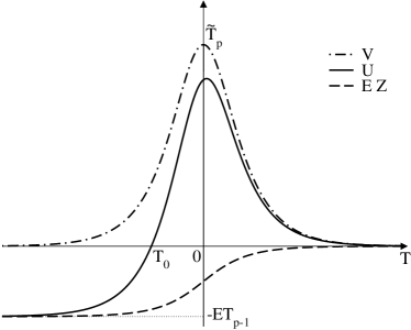
Figure 1: Tachyon potential $U(T)$ and functions $V(T)$ and $EZ(T)$.

However, since $U(-\infty)=-E\,T_{p-1}$, $T=+\infty$ is a metastable vacuum and will tunnel to the true vacuum at $T=-\infty$ (see FIG. 1). On the other hand, from the asymptotics of $V$ and $Z$ it is also clear that, as one increases $E$ above a critical value, $T=+\infty$ ceases to be a metastable vacuum. The critical field depends on the specific form of $V$ and $W$, but it will be of order the string scale. For the particular choice (2) the critical value is $1/\sqrt{2}$.

In the above language it is easy to check that the kink representing a D$(p-1)$–brane feels a force due to the external field. Consider a configuration depending on a single variable $x^{p}$ with $T(\pm\infty)=\pm\infty$. Then, under a translation $x^{p}\to x^{p}+\delta x^{p}$, the change in the energy density is $\delta x^{p}EU(-\infty)$, which gives the constant pressure $ET_{p-1}$.

Since $T=+\infty$ is metastable one expects that there is a finite rate per unit time and volume for the nucleation of bubbles of the true vacuum inside the false vacuum. Furthermore, we see that the surface of the bubble is the locus where the tachyon field interpolates between the two minima, and should therefore be interpreted as a spherical D$(p-1)$–brane. We will estimate the nucleation rate using the standard semiclassical methods developed by Coleman. This amounts to finding the bounce: the non–trivial classical solution of the Euclidean equations of motion, which approaches the false vacuum at infinity and has minimal Euclidean action $S_{0}$. Then $\Gamma/V\simeq\Delta\,e^{-S_{0}}$ is the nucleation rate per unit time and $p$–volume, with $\Delta$ a pre–factor. This pre–factor is related to the determinant of the open string field fluctuations around the bounce. Since the tachyon classical action is obtained by eliminating the massive open string fields via their equations of motion, the naive pre-factor computed from the action (1) would neglect fluctuations of the massive string modes.

Since the kinetic term in the action is not canonical, one should verify the validity of standard instanton methods for the Born-Infeld Euclidean action

$$S_{E}=\int d^{p+1}x\,\left[V(T)\sqrt{1+(\partial T)^{2}}+E\,Z(T)\right].$$

Let us call the bounce solution $\bar{T}$ and define a one–parameter family of functions $T_{\lambda}(x)\equiv\bar{T}(x/\lambda)$. One can easily show that

$$\left.\frac{d}{d\lambda}\,S_{E}\left[T_{\lambda}\right]\right|_{\lambda=1}= (p+1)\,S_{E}\left[\bar{T}\right]$$

$$-\int d^{p+1}x\,\frac{V(\bar{T})(\partial\bar{T})^{2}}{\sqrt{1+(\partial\bar{T})^{2}}}\ .$$

Since $\lambda=1$ is a stationary point of the action it follows that $S_{E}\left[\bar{T}\right]>0$. One may also compute the second derivative at $\lambda=1$ and easily show that it is negative. This fact guarantees the existence of a negative eigenmode in the quadratic fluctuations around the bounce. One also expects that the bounce is spherically symmetric and that it has precisely one negative eigenmode.

To simplify the analysis of the dynamics of the bounce, we shall work with potential functions ${\cal V},{\cal U},{\cal Z}$, which are obtained from the original $V,U,Z$ by rescaling them by $2/T_{p-1}$. Start by defining a new field

$$\Phi=\int_{0}^{T}\,{\cal V}(T^{\prime})\,dT^{\prime}\ ,$$

such that $T=\pm\infty$ corresponds to $\Phi=\pm 1$. For the particular choice (2), one has

$${\cal V}=\frac{\sqrt{2}}{\pi}\cos\left(\frac{\pi}{2}\,\Phi\right)\ ,\ \ \ \ \ \ \ \ \ \ {\cal Z}=\Phi-1\ .$$ (3)

For a Euclidean solution with maximal symmetry $\Phi=\Phi(r)$ where $r^{2}=x_{\mu}x^{\mu}$, the effective one–dimensional action reads

$$I_{E}=\int_{0}^{\infty}dr\,r^{p}\left[\sqrt{{\cal V}^{2}+\dot{\Phi}^{2}}+E\,{\cal Z}\right]\ ,$$

where dot denotes the radial derivative. The Euclidean action is $S_{E}=I_{E}A_{p}T_{p-1}/2$, with $A_{p}$ the volume of the $p$–sphere.

The equations of motion turn out to be simpler in the Hamiltonian formulation. The conjugate momentum to the field $\Phi$ is related to

$$\frac{1}{r^{p}}\,\frac{\partial L}{\partial\dot{\Phi}}=\frac{\dot{\Phi}}{\sqrt{{\cal V}^{2}+\dot{\Phi}^{2}}}\equiv\Pi\ .$$

Thus, since ${\cal V}$ is non–negative, the variable $\Pi$ is also bounded between $-1$ and $1$. Finally, the equations of motion reduce to the following dynamical system

$$\dot{\Pi} = {\cal V}^{\prime}(\Phi)\sqrt{1-\Pi^{2}}+E\,{\cal Z}^{\prime}(\Phi)-\frac{p}{r}\,\Pi\ ,$$

$$\dot{\Phi} = \frac{{\cal V}(\Phi)\,\Pi}{\sqrt{1-\Pi^{2}}}\ .$$ (4)

Although for $p>0$ the system is not conservative, it is still useful to consider the Hamiltonian

$$-\frac{1}{r^{p}}\,H={\cal V}(\Phi)\sqrt{1-\Pi^{2}}+E\,{\cal Z}(\Phi)\equiv K\ .$$

Using (4) it is easy to show that

$$\dot{K}=\frac{p}{r}\frac{{\cal V}(\Phi)\Pi^{2}}{\sqrt{1-\Pi^{2}}}\geq 0\ .$$

Thus, it is instructive to consider the $K$ contour plot, since $K$ never decreases along the $(\Phi(r),\Pi(r))$ trajectories (see FIG. 2). Spherical symmetry demands $\Pi(0)=0$ and therefore all trajectories start from the $\Pi=0$ horizontal axis.

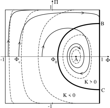
Figure 2: Contour plot of $K$ and typical trajectories for $E>E_{c}$. The thick line is the $K=0$ contour and the dashed lines are other $K$ contours. The line starting at $\Phi_{c}$ is the bounce for $p>0$ and the other two lines are typical trajectories. When $E\leq E_{c}$ the bounce degenerates to the boundary of phase space.

Consider first the conservative case $p=0$, where the trajectories follow lines of constant $K$ clockwise. The bounce solution is the trajectory with $K=0$, with the initial value $\Phi_{0}$ defined by the equation $K(\Phi_{0},0)={\cal U}(\Phi_{0})=0$. This trajectory approaches the vertical line $\Phi=1$ as $r\to\infty$ (point B in FIG. 2). The corresponding Euclidean action is given by the integral

$$S_{0}=T_{p-1}\int_{\Phi_{0}}^{1}d\Phi\sqrt{1-\left(\frac{E\,{\cal Z}}{{\cal V}}\right)^{2}}\ .$$

In the limit $E\to 0$ the above action remains finite and describes a $D/\bar{D}$–instanton pair. Trajectories that start with $\Phi(0)$ between $\Phi_{0}$ and $1$ are periodic and those that start between $-1$ and $\Phi_{0}$ end in finite $r$ at the horizontal line $\Pi=1$.

Next we consider the case $p>0$. Now all trajectories that enter the $K>0$ region will inevitably approach point $A$ in FIG. 2 at $r=\infty$. This will happen for $\Phi(0)$ greater than some critical value $\Phi_{c}$ satisfying $-1\leq\Phi_{c}<\Phi_{0}$. On the other hand, trajectories with $\Phi(0)<\Phi_{c}$ reach $\Pi=1$ in finite $r$ and can not be continued further. The bounce is precisely the solution with $\Phi(0)=\Phi_{c}$. To understand the behavior of $\Phi_{c}$ as a function of the electric field $E$, let us look at the extreme solution with $\Phi(0)=-1$. This trajectory stays in the vertical line $\Phi=-1$ until it hits $\Pi=1$ at a finite radius $\bar{r}$. Expanding the solution around this point, one can show that, for

$$E>E_{c}=\sqrt{\frac{p}{8}}\,\frac{1}{{\cal Z}^{\prime}(-1)}\ ,$$

we necessarily have $\dot{\Pi}(\bar{r})>0$ and therefore the trajectory ends. We conclude that for $E>E_{c}$ the bounce starts with $\Phi_{c}>-1$ and approaches point $B$ in FIG. 2 at $r=\infty$. This behavior is analogous to the case $p=0$, where the electric field is always above $E_{c}$. Although this solution is interesting, it is not clear if it survives string corrections. As $E$ decreases to $E_{c}$ the bounce trajectory degenerates to the boundary of the phase space. For $E\leq E_{c}$ the solution starts at $\Phi_{c}=-1$ and hits $\Pi=1$ at a radius $R=p/E$, where $\dot{\Pi}$ vanishes. Then the trajectory jumps discontinuously to $\Phi=\Pi=1$ and descends vertically to point $B$ in Fig. 2. As a function of $r$, the tachyon field $\Phi$ jumps discontinuously from the true to the false vacuum at $r=R$, while $\Pi(r)$ is smooth. We conclude that in this case the thin wall approximation is exact. This is a consequence of the kinetic term of Born–Infeld type. The Euclidean action of the bounce can then be explicitly evaluated

$$S_{0}=\frac{A_{p}}{p+1}\,T_{p-1}\,R^{p}\ .$$

This result was obtained by Teitelboim almost 20 years ago using first quantized $p$-brane mechanics Teitelboim . Here we have derived it as the bubble decay of the tachyon false vacuum for the case of D-brane nucleation in string theory.

The time evolution of the nucleated branes is determined by the analytic continuation of the bounce solution. For $p>0$ a $D(p-1)$–brane appears as a $(p-1)$–sphere of radius $R$ and then expands with constant radial acceleration $1/R$ describing a hyperboloid in Minkowski space. In this case all the energy arising from the decay of the false vacuum is transfered to the brane. For $p=0$ there is no brane to absorb the energy and therefore the tachyon field can not appear exactly in the true vacuum. In this case the tachyon field rolls down classically from $T_{0}$ (see FIG. 1) to the true vacuum.

After nucleation the brane will act as a source for closed strings. The tadpoles for the closed string fields can be computed by coupling the action (1) to these fields. Since the transverse coordinates of the original non–BPS brane vanish at the bounce, the only non–vanishing components of the sources for the metric and RR $p$–form field lie along the non–BPS brane world–volume. A simple computation shows that the metric, RR $p$–form and dilaton tadpoles are

$$T_{\mu\nu} = T_{p-1}\left(\frac{x_{\mu}x_{\nu}}{R^{2}}-\eta_{\mu\nu}\right)\delta(r-R)\,\delta_{\perp}(x)\ ,$$

$$J_{\mu_{1}\cdots\mu_{p}} = T_{p-1}\,\frac{x^{\nu}}{R}\,\epsilon_{\nu\mu_{1}\cdots\mu_{p}}\,\delta(r-R)\,\delta_{\perp}(x)\ ,$$

$$Q = T_{p-1}\,\delta(r-R)\,\delta_{\perp}(x)\ ,$$

where $r^{2}=x_{\mu}x^{\mu}$ is the analytic continuation of the Euclidean radial coordinate and $\delta_{\perp}(x)$ is a delta function on the transverse space. These are the sources that describe the decay of a RR flux $p$–brane. The linearized solution for the closed fields can be solved in terms of retarded Green functions and describes the radiation emitted by the expanding nucleated brane. This process can also be described in the framework of Euclidean quantum gravity using generalizations of the Ernst metric Dowker ; CostaGutperle . Here, instead of an effective closed string description, we used open strings to describe the decay process and the sources for the emitted radiation.

When the transverse directions to the non–BPS brane are compact, the delta functions $\delta_{\perp}(x)$ in the above sources should be replaced by the inverse of the volume of the transverse space. The sources induce a jump in the derivative of the dilaton, gauge potential and metric. Moreover, the dilaton will radiate. In the dimensionally reduced theory the jump in the electric field corresponds to the decay of a quintessence potential. It would be interesting to consider the explicit form of the background geometry and analyze the decay process throughout the cosmological evolution.

The techniques explored in this paper can also be applied to black hole physics. In particular, one could try to make predictions regarding the emission of branes by non–extremal black holes in string theory.

This work was supported in part by INFN, by the MIUR–COFIN contract 2003–023852, by the EU contracts MRTN–CT–2004–503369, MRTN–CT–2004–512194 and MERG–CT–2004–511309, by the INTAS contract 03–51–6346, by the NATO grant PST.CLG.978785 and by the FCT contracts POCTI/FNU/38004/2001 and POCTI/FP/FNU/50161/2003. L.C. is supported by the MIUR contract “Rientro dei cervelli” part VII and J.P. by the FCT fellowship SFRH/BD/9248/2002.

References

- (1) J.S. Schwinger, Phys. Rev. 82 (1951) 664.
- (2) C. Teitelboim, Phys. Lett. 167B (1986) 63.
- (3) A.Sen, [arXiv:hep-th/0410103].
- (4) S. Coleman, Phys. Rev D15 (1977) 2929.
- (5) K. Hashimoto, JHEP 0207 035.
- (6) C.G. Callan and J.M. Maldacena, Nucl. Phys. B 513 (1998) 198; K.G. Savvidy, [arXiv:hep-th/9810163].
- (7) P.M. Saffin, Phys. Rev. D 64 (2001) 024014; M. Gutperle and A. Strominger, JHEP 0106 035; M.S. Costa, C.A.R. Herdeiro and L. Cornalba, Nucl. Phys. B 619 (2001) 155.
- (8) L. Cornalba, M.S. Costa and C. Kounnas, Nucl. Phys. B 637 (2002) 378.
- (9) J.D. Brown and C. Teitelboim, Phys. Lett. B 195 (1987) 177.
- (10) F. Dowker, J.P. Gauntlett, G.W. Gibbons and G.T. Horowitz, Phys. Rev. D 53 (1996) 7115.
- (11) M.S. Costa and M. Gutperle, JHEP 0103 027.