Self-adjoint extensions and SUSY breaking in Supersymmetric Quantum Mechanics

Abstract.

We consider the self-adjoint extensions (SAE) of the symmetric supercharges and Hamiltonian for a model of SUSY Quantum Mechanics in $\mathbb{R}^{+}$ with a singular superpotential. We show that only for two particular SAE, whose domains are scale invariant, the algebra of $N=2$ SUSY is realized, one with manifest SUSY and the other with spontaneously broken SUSY. Otherwise, only the $N=1$ SUSY algebra is obtained, with spontaneously broken SUSY and non degenerate energy spectrum.

PACS numbers: 11.30.Pb, 03.65.Db, 02.30.Tb, 02.30.Sa

Mathematical Subject Classification: 81Q10, 34L40, 34L05

1. Introduction

Supersymmetry (SUSY) [1, 2, 3, 4, 5, 6, 8, 9, 10, 11] gives desirable features to quantum field theories, like an improved ultraviolet behavior, but also predicts superpartner states with degenerate mass which are not observed experimentally. Therefore, this symmetry is expected to be spontaneously (dynamically) broken.

Several schemes have been developed to try to solve the SUSY breaking problem, including the idea of non-perturbative breaking by instantons. In this context, the simplest case of SUSY Quantum Mechanics (SUSYQM) was introduced by Witten [8] and Cooper and Freedman [10].

When considering these models, several authors have suggested that singular potentials could break SUSY through nonstandard mechanisms, being responsible for non degeneracy of energy levels and negative energy eigenstates [12, 13, 14, 15, 16, 17].

In particular, Jevicki and Rodrigues [12] have considered the singular superpotential $W(x)=g/x-x$. Based on the square integrable solutions of a differential operator related to the Hamiltonian of this system [18] they concluded that, for a certain range of the parameter $g$, SUSY is broken with a negative energy ground state.

However, they have not considered if all these functions correspond to eigenvectors of a unique self-adjoint Hamiltonian. As is well known, the quantum dynamics is given by a unitary group, and it follows from Stone’s theorem [19] that the Hamiltonian, which is the infinitesimal generator of this group, must be self-adjoint.

Later, Das and Pernice [20] have reconsidered this problem in the framework of a SUSY preserving regularization of the singular superpotential, finding that SUSY is recovered manifestly at the end, when the regularization is removed. They conclude that SUSY is robust at short distances (high energies), and the singularities that occur in quantum mechanical models are unlike to break SUSY.

In the present article we would like to address this controversial subject by studying the self-adjoint extensions of the Hamiltonian defined by the singular superpotential $W(x)=g/x-x$ with $x\in\mathbb{R}^{+}$. This will be done by studying the self-adjoint extensions of the symmetric supercharges, and by considering the possibility of realizing the algebra of SUSY in a dense subspace of the Hilbert space.

We will show that there is a range of values of $g$ for which the supercharges admit a one-parameter family of self-adjoint extensions, corresponding to a one-parameter family of self-adjoint extensions of the Hamiltonian. We will show that only for two particular self-adjoint extensions, whose domains are scale invariant, the algebra of $N=2$ SUSY can be realized, one with manifest SUSY and the other with spontaneously broken SUSY. For other values of this continuous parameter, only the $N=1$ SUSY algebra is obtained, with spontaneously broken SUSY and non degenerate energy spectrum.

We should mention that self-adjoint extensions of supercharges and Hamiltonian for the SUSYQM of the free particle with a point singularity in the line and the circle have been considered in [21, 22, 23, 24], where $N=1,2$ realization of SUSY are described. They have also been considered in the framework of the Landau Hamiltonian for two-dimensional particles in nontrivial topologies in [25] (see also [26]).

Let us remark that, given a superpotential $W(x)$, one gets a formal expression for the Hamiltonian (and also for the supercharges) as a symmetric differential operator $H$ defined on a subspace of sufficiently smooth square-integrable functions. The theory of deficiency indices of von Neumann [19] gives the basic criterion for the existence of self-adjoint extensions of this operator. In the case where there is only one self-adjoint extension, $H$ is essentially self-adjoint and its closure [19] represents the true Hamiltonian of the system. But if there are several self-adjoint extensions of $H$, they usually differ by the physics they describe. In this case, the election of a Hamiltonian among the self-adjoint extensions of $H$ is not just a mathematical technicality. Rather, additional physical information is required to select the correct one, that which describes the true properties of the system.

The structure of the paper is as follows: In the next Section we present the problem to solve. In Section 3 we study the adjoint operator of the supercharge, whose properties are needed to determine the supercharge self-adjoint extensions. This is done in Section 4, where the self-adjoint extensions of the Hamiltonian are also determined. In Section 5 we consider the possibility of realizing the algebra of the supersymmetry on the Hamiltonian domain of definition, and state our conclusions. In Appendix A we treat some technicalities related to the closure of the symmetric supercharge and in Appendix B we consider the graded partition function and the Witten index of the Hamiltonian, and the spectral asymmetry of the supercharge.

2. Setting of the problem

The Hamiltonian of a supersymmetric one-dimensional system can be written as

(2.1) $$H=\{\mathcal{Q},\widetilde{\mathcal{Q}}\}_{+},$$

where the supercharges

(2.6) $$\mathcal{Q}=\left(\begin{array}[]{cc}0&0\\ A&0\end{array}\right),\quad\widetilde{\mathcal{Q}}=\left(\begin{array}[]{cc}0&\widetilde{A}\\ 0&0\end{array}\right)$$

are nilpotent operators,

(2.7) $$\mathcal{Q}^{2}=\widetilde{\mathcal{Q}}^{2}=0,$$

which commute with the Hamiltonian.

In eq. (2.6),

(2.8) $$A=\displaystyle{\frac{1}{\sqrt{2}}\left(-\frac{d}{dx}+W(x)\right)}\quad{\rm and}\quad\widetilde{A}=\displaystyle{\frac{1}{\sqrt{2}}\left(\frac{d}{dx}+W(x)\right)}$$

are differential operators defined on a suitable dense subspace of functions where the necessary compositions of operators in Eqs. (2.1) and (2.7) are well defined, and $W(x)$ is the superpotential.

In this Section we will consider a quantum mechanical system living in the half line $\mathbf{R^{+}}$, subject to a superpotential given by

(2.9) $$W(x)=\frac{g}{x}-x$$

for $x>0$ and $g$ real. The two differential operators defined in (2.8) take the form

(2.10) $$A=\frac{1}{\sqrt{2}}\left(-\frac{d}{dx}+\frac{g}{x}-x\right),$$

(2.11) $$\widetilde{A}=\frac{1}{\sqrt{2}}\left(\frac{d}{dx}+\frac{g}{x}-x\right).$$

Let us now introduce an operator $Q_{+}$, defined on the dense subspace of (two component) functions with continuous derivatives of all order and compact support not containing the origin, $\mathcal{D}(Q_{+})=\mathcal{C}^{\infty}_{0}(\mathbf{R^{+}\backslash\{0\}})$, over which its action is given by

(2.12) $$Q_{+}\Psi=\left(\begin{array}[]{cc}0&\widetilde{A}\\ A&0\end{array}\right)\left(\begin{array}[]{c}\psi_{1}\\ \psi_{2}\\ \end{array}\right).$$

Notice that, within this domain, $Q_{+}$ can be identified with

(2.13) $$Q_{+}=\widetilde{\mathcal{Q}}+\mathcal{Q},$$

while its square (which is well defined) satisfies

(2.14) $$Q_{+}^{2}=\{\mathcal{Q},\widetilde{\mathcal{Q}}\}_{+}=H=\left(\begin{array}[]{cc}H_{+}&0\\ 0&H_{-}\end{array}\right),$$

where $H$ is the Hamiltonian of the system, with $H_{+}=\widetilde{A}A$ and $H_{-}=A\widetilde{A}$.

It can be easily verified that $Q_{+}$ so defined is a symmetric operator, but it is neither self-adjoint nor even closed. Consequently, we must look for the self-adjoint extensions of $Q_{+}$.

Within the same domain, a linearly independent combination of supercharges leads to the operator

(2.15) $$Q_{-}=i(\widetilde{\mathcal{Q}}-\mathcal{Q}),$$

which is also symmetric and satisfies that $Q_{-}^{2}=H$, and $\left\{Q_{+},Q_{-}\right\}_{+}=0$. Since it can be obtained from $Q_{+}$ through a unitary transformation given by

(2.16) $$Q_{-}=e^{i\sigma_{3}\pi/4}Q_{+}e^{-i\sigma_{3}\pi/4},\ {\rm with}\ \sigma_{3}=\left(\begin{array}[]{cc}1&0\\ 0&-1\end{array}\right),$$

the following analysis will be carried out only for $Q_{+}$, and it will extend immediately to $Q_{-}$.

Notice that, given a self-adjoint extension of $Q_{+}$ (which, in particular, is a closed and densely defined operator [19]), its square gives the corresponding self-adjoint extension of the Hamiltonian $H$ in Eq. (2.14), by virtue of a theorem due to von Neumann [27].

The first step in the construction of the self-adjoint extensions of $Q_{+}$ consists in the determination of its adjoint, $Q_{+}^{\dagger}$, which will be done in the next Section.

3. The adjoint operator $Q_{+}^{\dagger}$

In this Section we will determine the domain of definition of $Q_{+}^{\dagger}$, and its spectrum. In particular, we are interested in the deficiency subspaces [19] of $Q_{+}$ (the null subspaces of $(Q_{+}^{\dagger}\mp i)$),

(3.1) $$\mathcal{K}_{\pm}:={\rm Ker}(Q_{+}^{\dagger}\mp i),$$

which determine the self-adjoint extensions of $Q_{+}$.

3.1. Domain of $Q_{+}^{\dagger}$

A (two component) function $\Phi$ belongs to the domain of $Q_{+}^{\dagger}$,

(3.2) $$\Phi=\left(\begin{array}[]{c}\phi_{1}\\ \phi_{2}\end{array}\right)\in\mathcal{D}(Q_{+}^{\dagger})\subset\mathbf{L_{2}}(\mathbb{R^{+}}),$$

if $\left(\Phi,Q_{+}\Psi\right)$ is a linear continuous functional of $\Psi$, for $\Psi\in\mathcal{D}(Q_{+})$. This requires the existence of a function

(3.3) $$\Omega=\left(\begin{array}[]{c}\chi_{1}\\ \chi_{2}\end{array}\right)\in\mathbf{L_{2}}(\mathbb{R^{+}})$$

such that

(3.4) $$\left(\Phi,Q_{+}\Psi\right)=\left(\Omega,\Psi\right),\ \forall\Psi\in\mathcal{D}(Q_{+}).$$

Such $\Omega$ is uniquely determined, since $\mathcal{D}(Q_{+})$ is a dense subspace. Then, for each $\Phi\in\mathcal{D}(Q_{+}^{\dagger})$, the action of $Q_{+}^{\dagger}$ is defined by $Q_{+}^{\dagger}\Phi:=\Omega$. Notice that $\mathcal{D}(Q_{+})\subset\mathcal{D}(Q_{+}^{\dagger})$, since $Q_{+}$ is symmetric.

We will now determine the properties of the functions in $\mathcal{D}(Q_{+}^{\dagger})$, and the way $Q_{+}^{\dagger}$ acts on them. In a distributional sense, Eq. (3.4) implies that

(3.5) $$\displaystyle{-\phi_{1}^{\prime}+\left({g\over x}-x\right)\phi_{1}=\sqrt{2}\,\chi_{2}},$$

(3.6) $$\displaystyle{\phi_{2}^{\prime}+\left({g\over x}-x\right)\phi_{2}=\sqrt{2}\,\chi_{1}},$$

which shows that $\Phi^{\prime}(x)$ is a regular (locally integrable) distribution. This implies that $\Phi(x)$ is an absolutely continuous function for $x>0$.

Therefore, the domain of $Q_{+}^{\dagger}$ consists on those (square-integrable) absolutely continuous functions such that the left hand sides in Eqs. (3.5) and (3.6) are also square-integrable functions on the half-line:

(3.7) $$\begin{array}[]{c}\mathcal{D}(Q_{+}^{\dagger})=\{\Phi\in AC(\mathbb{R^{+}}\backslash\{0\})\cap\mathbf{L_{2}}(\mathbb{R^{+}}):\\ \\ A\,\phi_{1},\,\widetilde{A}\,\phi_{2}\in\mathbf{L_{2}}(\mathbb{R^{+}})\}.\end{array}$$

Consequently, an integration by parts in the left hand side of Eq. (3.4) is justified, and we conclude that the action of $Q_{+}^{\dagger}$ on $\Phi\in\mathcal{D}(Q_{+}^{\dagger})$ also reduces to the application of the differential operator

(3.8) $$Q_{+}^{\dagger}\Phi=\left(\begin{array}[]{cc}0&\widetilde{A}\\ A&0\end{array}\right)\left(\begin{array}[]{c}\phi_{1}\\ \phi_{2}\\ \end{array}\right).$$

3.2. Spectrum of $Q_{+}^{\dagger}$

We now consider the eigenvalue problem for $Q_{+}^{\dagger}$,

(3.9) $$Q_{+}^{\dagger}\Phi_{\lambda}=\lambda\Phi_{\lambda},$$

or equivalently

(3.10) $$A\,\phi_{1}=\lambda\,\phi_{2},\quad\widetilde{A}\,\phi_{2}=\lambda\,\phi_{1},$$

with

(3.11) $$\Phi_{\lambda}=\left(\begin{array}[]{c}\phi_{1}\\ \phi_{2}\end{array}\right)\in\mathcal{D}(Q_{+}^{\dagger})$$

and $\lambda\in\mathbb{C}$.

From Eqs. (2.10), (2.11) and (3.10), it follows immediately that $\Phi_{\lambda}^{\prime}(x)$ is an absolutely continuous function. In fact, the successive applications of $Q_{+}^{\dagger}$ on both sides of Eq. (3.9) show that $\Phi_{\lambda}(x)\in\mathcal{C}^{\infty}(\mathbb{R^{+}}\backslash\{0\})$, and Eq. (3.10) is just a system of ordinary differential equations.

Replacing $\phi_{2}$ in terms of $\phi_{1}$ we get

(3.12) $$-\frac{1}{2}\,\phi_{1}^{\prime\prime}+\frac{1}{2}\left\{\frac{g(g-1)}{x^{2}}+x^{2}-1-2g\right\}\phi_{1}=\lambda^{2}\,\phi_{1},$$

(3.13) $$\lambda\,\phi_{2}=\frac{1}{\sqrt{2}}\left\{-\phi_{1}^{\prime}+\left(\frac{g}{x}-x\right)\phi_{1}\right\}.$$

Making the substitution

(3.14) $$\phi_{1}(x)=x^{g}\,e^{{-{x^{2}/2}}}\,F(x^{2})$$

in Eq. (3.12) we get the Kummer’s equation [28] for $F(z)$,

(3.15) $$z\,F^{\prime\prime}(z)+(b-z)\,F^{\prime}(z)-a\,F(z)=0,$$

with

(3.16) $$a=-\frac{\lambda^{2}}{2},\quad b=g+\frac{1}{2}.$$

For any values of the parameters $a$ and $b$, equation (3.15) has two linearly independent solutions [28] given by the Kummer’s function

(3.17) $$\begin{array}[]{c}y_{1}(z)=U(a,b,z)=\\ \\ \displaystyle{\frac{\pi}{\sin\pi b}\left\{\frac{M(a,b,z)}{\Gamma(1+a-b)\Gamma(b)}-z^{1-b}\,\frac{M(1+a-b,2-b,z)}{\Gamma(a)\Gamma(2-b)}\right\}},\end{array}$$

and

(3.18) $$y_{2}(z)=e^{z}\,U(b-a,b,-z).$$

In Eq. (3.17), $M(a,b,z)={{}_{1}F_{1}(a;b;z)}$ is the confluent hypergeometric function.

Since for large values of the argument [28]

(3.19) $$U(a,b,z)=z^{-a}\left\{1+\mathcal{O}(|z|^{-1})\right\},$$

only $y_{1}(x^{2})$ leads to a function $\phi_{1}(x)\in\mathbf{L_{2}}(1,\infty)$ when replaced in Eq. (3.14), while $y_{2}(x^{2})$ should be discarded.

Therefore, we get

(3.20) $$\phi_{1}(x)=x^{g}\,e^{{-{x^{2}/2}}}\,U(-\frac{\lambda^{2}}{2},g+\frac{1}{2},x^{2}).$$

On the other hand, replacing Eq. (3.20) in Eq. (3.13), it is straightforward to show that [28]

(3.21) $$\phi_{2}(x)=-\frac{\lambda}{\sqrt{2}}\,x^{g+1}\,e^{-{x^{2}}/{2}}\,U(1-\frac{\lambda^{2}}{2};g+\frac{3}{2},x^{2}),$$

which is also in $\mathbf{L_{2}}(1,\infty)$.

In order to determine the spectrum of $Q_{+}^{\dagger}$, we must now consider the behavior of $\Phi_{\lambda}(x)=\left(\begin{array}[]{c}\phi_{1}(x)\\ \phi_{2}(x)\end{array}\right)$ near the origin. From Eq. (3.17), and the small argument expansion of Kummer’s functions (see [28], page 508), one can straightforwardly show that three cases should be distinguished, according to the values of the coupling $g$:

• If $g\geq 1/2$, it can be seen that $\Phi_{\lambda}(x)\notin\mathbf{L_{2}}(0,1)$ unless $-\lambda^{2}/2=-n$, with $n=0,1,2,\dots$ In this case, taking into account that $U(-n,b,z)$ reduces to a Laguerre polynomial (of degree $n$ in $z$),

  (3.22) $$U(-n,b,z)=(-1)^{n}\,n!\,L_{n}^{(b-1)}(z),$$

  we have $\phi_{1}(x)\sim x^{g}$ and $\phi_{2}(x)\sim x^{g+1}$ for $0<x\ll 1$ (Notice that the square-integrability of $\phi_{1}(x)$ and $\phi_{2}(x)$ on $\mathbb{R}^{+}$ is guaranteed by the decreasing exponentials in Eqs. (3.20) and (3.21)). Therefore, in this region $Q_{+}^{\dagger}$ has a symmetric real spectrum given by the (degeneracy one) eigenvalues

  (3.23) $$\lambda_{0}=0,\quad\lambda_{\pm,n}=\pm\sqrt{2n},\quad n=1,2,3,\dots$$

  corresponding to the eigenfunctions

  (3.24) $$\Phi_{0}=x^{g}\,e^{{-{x^{2}/2}}}\left(\begin{array}[]{c}1\\ 0\end{array}\right),$$

  and

  (3.25) $$\Phi_{\pm,n}=(-1)^{n}\,n!\,x^{g}\,e^{{-{x^{2}/2}}}\left(\begin{array}[]{c}L_{n}^{(g-\frac{1}{2})}(x^{2})\\ \\ \mp\displaystyle{\frac{x}{\sqrt{n}}}\,L_{n-1}^{(g+\frac{1}{2})}(x^{2})\end{array}\right)$$

  respectively.

• For $-1/2<g<1/2$, it can be seen from (3.20), (3.21) and (3.17) that $\Phi_{\lambda}(x)\in\mathbf{L_{2}}(0,1)$, $\forall\lambda\in\mathbb{C}$. This means that, for these values of $g$, every complex number is an eigenvalue of $Q_{+}^{\dagger}$ with degeneracy one. For example, the eigenfunction of $Q_{+}^{\dagger}$ corresponding to $\lambda=i$ is given by

  (3.26) $$\begin{array}[]{c}\Phi_{\lambda=i}(x)=\Phi_{+}(x)=\left(\begin{array}[]{c}\phi_{+,1}\\ \phi_{+,2}\end{array}\right)=\\ \\ =x^{g}\,e^{{-{x^{2}/2}}}\left(\begin{array}[]{c}U\left(\frac{1}{2},g+\frac{1}{2},x^{2}\right)\\ \\ -\frac{i}{\sqrt{2}}\,x\,U\left(\frac{3}{2},g+\frac{3}{2},x^{2}\right)\end{array}\right),\end{array}$$

  while the eigenfunction corresponding to $\lambda=-i$ is given by its complex conjugate,

  (3.27) $$\Phi_{\lambda=-i}(x)=\Phi_{-}(x)=\Phi_{+}(x)^{*}$$

  (since the coefficients in the differential operators in Eq. (3.10) are real).

• Finally, for $g\leq-1/2$, it can be seen that $\Phi_{\lambda}(x)\notin\mathbf{L_{2}}(0,1)$ unless $-\lambda^{2}/2=g-\frac{1}{2}-n$, with $n=0,1,2,\dots$ In this case, taking into account the Kummer transformation (see [28], page 505),

  (3.28) $$U(1-n-b,2-b,z)=z^{b-1}\,U(-n,b,z),$$

  and Eq. (3.22), we have $\phi_{1}(x)\sim x^{1-g}$ and $\phi_{2}(x)\sim x^{-g}$ for $0<x\ll 1$. Therefore, in this region $Q_{+}^{\dagger}$ has a symmetric real spectrum given by the (degeneracy one) eigenvalues

  (3.29) $$\lambda_{\pm,n}=\pm\sqrt{2n+1-2g},\quad n=0,1,2,\dots$$

  corresponding to the eigenfunctions

  (3.30) $$\begin{array}[]{c}\Phi_{\pm,n}=(-1)^{n}\,n!\times\\ \\ x^{-g}\,e^{{-{x^{2}/2}}}\left(\begin{array}[]{c}x\,L_{n}^{(\frac{1}{2}-g)}(x^{2})\\ \\ \mp\sqrt{n+\frac{1}{2}-g}\,L_{n}^{(-g-\frac{1}{2})}(x^{2})\end{array}\right).\end{array}$$

  Notice that no eigenvalue vanishes for these values of the coupling.

These results will be employed in the next Section to determine the self-adjoint extensions of $Q_{+}$.

4. Self-adjoint extensions of $Q_{+}$

According to von Neumann’s theory [19], to construct the self-adjoint extensions of $Q_{+}$ we must take into account the different behaviors of $Q_{+}^{\dagger}$, described in the previous Section.

4.1. For $|g|\geq 1/2$ the operator $Q_{+}$ is essentially self-adjoint

As seen in Section 3.2, the deficiency indices [19] of $Q_{+}$, defined as the dimensions of the deficiency subspaces $\mathcal{K}_{\pm}$,

(4.1) $$n_{\pm}:={\rm dim}\ {\rm Ker}(Q_{+}^{\dagger}\mp i),$$

vanish for $|g|\geq 1/2$. This means that $Q_{+}$ is essentially self-adjoint [19] in these regions of the coupling, admitting there a unique self-adjoint extension given by $Q_{+}^{\dagger}$ (which, in this case, is itself a self-adjoint operator).

The corresponding self-adjoint extension of the Hamiltonian in Eq. (2.14) is given by [27]

(4.2) $$\overline{H}=(Q_{+}^{\dagger})^{2},$$

where the operator composition in the right hand side is possible in the dense domain

(4.3) $$\mathcal{D}(\overline{H})=\left\{\psi\in\mathcal{D}(Q_{+}^{\dagger}):Q_{+}^{\dagger}\psi\in\mathcal{D}(Q_{+}^{\dagger})\right\}.$$

Notice that every eigenfunctions of $Q_{+}^{\dagger}$, corresponding to an eigenvalue $\lambda$, belongs to $\mathcal{D}\left(\overline{H}\right)$. Therefore, it is also an eigenfunction of $\overline{H}$ with eigenvalue $E=\lambda^{2}$. So, we have:

• For $g\geq 1/2$, the eigenfunctions of $\overline{H}$ are given in Eqs. (3.24) and (3.25). Notice that there is a unique zero mode, while the positive eigenvalues of $\overline{H}$,

  (4.4) $$E_{n}=2\,n,\quad n=1,2,3,\dots$$

  are doubly degenerate (see Eq. (3.23)). One can add and subtract the corresponding eigenfunctions in Eq. (3.25) to get bosonic and fermionic states (with only the upper and lower component non vanishing respectively). For these values of the coupling, the Witten index is $\Delta=1$ and the SUSY is manifest [8].

• For $g\leq-1/2$, the eigenfunctions of $\overline{H}$ are given in Eq. (3.30). Notice that there is no zero mode. Once again, the positive eigenvalues of $\overline{H}$,

  (4.5) $$E_{n}=2\,n+1-2\,g\geq 2,\quad n=0,1,2,\dots$$

  are doubly degenerate (see Eq. (3.29)), and the eigenfunctions can be combined to get bosonic and fermionic states. For these values of $g$, the SUSY is spontaneously broken and the Witten index is $\Delta=0$ [8].

4.2. For $|g|<1/2$ the operator $Q_{+}$ is not essentially self-adjoint

On the other hand, according to Eqs. (3.26) and (3.27) in Section 3.2, for $-1/2<g<1/2$ the deficiency indices are $n_{\pm}=1$. In this region $Q_{+}$ admits a one parameter family of self-adjoint extensions, $Q_{+}^{\gamma}$, which are in a one-to-one correspondence with the isometries from $\mathcal{K}_{+}$ onto $\mathcal{K}_{-}$ [19], characterized by

(4.6) $$\mathcal{U}(\gamma)\Phi_{+}(x):=e^{2i\gamma}\Phi_{-},\quad\gamma\in[0,\pi),$$

with $\Phi_{+}$ and $\Phi_{-}$ given in Eqs. (3.26) and (3.27) respectively.

The self-adjoint operator $Q_{+}^{\gamma}$ is the restriction of $Q_{+}^{\dagger}$ to a dense subspace

(4.7) $$\mathcal{D}(Q_{+}^{\gamma})\subset\mathcal{D}(Q_{+}^{\dagger})=\mathcal{D}(\overline{Q}_{+})\oplus\mathcal{K}_{+}\oplus\mathcal{K}_{-}$$

(here, $\overline{Q}_{+}$ is the closure of $Q_{+}$ [19]), composed by those functions which can be written as

(4.8) $$\Phi=\left(\begin{array}[]{c}\phi_{1}\\ \phi_{2}\end{array}\right)=\overline{\Phi}_{0}+c\left(\Phi_{+}+e^{2i\gamma}\Phi_{-}\right),$$

with $\overline{\Phi}_{0}=\left(\begin{array}[]{c}\phi_{0,1}\\ \phi_{0,2}\end{array}\right)\in\mathcal{D}(\overline{Q}_{+})$, and the constant $c\in\mathbb{C}$.

Obviously, we have

(4.9) $$Q_{+}^{\gamma}\Phi=Q_{+}^{\dagger}\overline{\Phi}_{0}+ic\left(\Phi_{+}-e^{2i\gamma}\Phi_{-}\right),$$

with $Q_{+}^{\dagger}$ given in Eq. (3.8).

Equation (4.8) completely characterizes the behavior near the origin of the functions $\Phi\in\mathcal{D}\left(Q_{+}^{\gamma}\right)$. As we will see, it also allows to determine the spectrum of $Q_{+}^{\gamma}$.

Indeed, in Appendix A we have worked out the domain of the closure of $Q_{+}$, $\mathcal{D}(\overline{Q}_{+})$, showing that

(4.10) $$\phi_{0,1}(x)={o}(x^{g}),\quad\phi_{0,2}(x)={o}(x^{-g}),$$

for $x\rightarrow 0^{+}$. On the other side, from Eqs. (3.11), (3.20), (3.21) and (3.17), one can easily see that the components of any eigenfunction $\Phi_{\lambda}$ of $Q_{+}^{\dagger}$ behave as

(4.11) $$\begin{array}[]{c}\phi_{1}(x)=\displaystyle{\frac{\Gamma\left(\frac{1}{2}-g\right)}{\Gamma\left(\frac{1-\lambda^{2}}{2}-g\right)}}\ x^{g}+O(x^{1-g}),\\ \\ \phi_{2}(x)=\displaystyle{\frac{\sqrt{2}}{\lambda}\ \frac{\Gamma\left(\frac{1}{2}+g\right)}{\Gamma\left(-\frac{\lambda^{2}}{2}\right)}}\ x^{-g}+O(x^{1+g}).\end{array}$$

Therefore, no eigenfunction of $Q_{+}^{\dagger}$ belongs to $\mathcal{D}(\overline{Q}_{+})$.

Consequently, it is the contributions of $\Phi_{\pm}$ in Eq. (4.8) which determine the spectrum of $Q_{+}^{\gamma}$. In fact, consider the limit

(4.12) $$\lim_{x\rightarrow 0+}\frac{x^{-g}\,\phi_{1}(x)}{x^{g}\,\phi_{2}(x)}=\displaystyle{\frac{\lambda}{\sqrt{2}}\,\frac{\Gamma\left(-\frac{\lambda^{2}}{2}\right)}{\Gamma\left(\frac{1-\lambda^{2}}{2}-g\right)}\frac{\Gamma\left(\frac{1}{2}-g\right)}{\Gamma\left(\frac{1}{2}+g\right)}}.$$

For a non vanishing $c$ in the right hand side of Eq. (4.8), this limit must coincide with

(4.13) $$\lim_{x\rightarrow 0+}\frac{\Re\left\{e^{-i\gamma}\,x^{-g}\,\phi_{+,1}(x)\right\}}{\Re\left\{e^{-i\gamma}\,x^{g}\,\phi_{+,2}(x)\right\}}=\displaystyle{-\sqrt{\frac{\pi}{2}}\,\frac{\cot(\gamma)}{\Gamma\left(1-g\right)}\frac{\Gamma\left(\frac{1}{2}-g\right)}{\Gamma\left(\frac{1}{2}+g\right)}},$$

where Eq. (3.27) and Eq. (4.11) with $\lambda\rightarrow i$ have been taken into account. Then, the eigenvalues of $Q_{+}^{\gamma}$ (which are real) are the solutions of the transcendental equation

(4.14) $${f(\lambda):=\frac{\lambda\,\Gamma\left(-\frac{\lambda^{2}}{2}\right)}{\Gamma\left(\frac{1-\lambda^{2}}{2}-g\right)}=-\frac{\sqrt{\pi}\,\cot(\gamma)}{\Gamma\left(1-g\right)}=:\beta(\gamma)}.$$

Notice that $f(\lambda)$ is an odd function of $\lambda$, and $-\infty\leq\beta(\gamma)<\infty$ for $0\leq\gamma<\pi$.

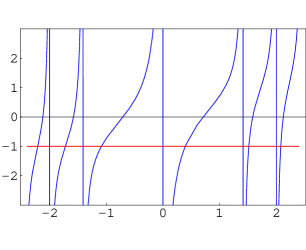
Figure 1. $f(\lambda):=\displaystyle{\frac{\lambda\,\Gamma\left(-\frac{\lambda^{2}}{2}\right)}{\Gamma\left(\frac{1-\lambda^{2}}{2}-g\right)}}$ for $g=1/4$, and $\beta(\gamma)\equiv-1$.

The function $f(\lambda)$ in the left hand side of Eq. (4.14) has been plotted in Fig. 1, for a value of the coupling $g=1/4$. The eigenvalues of $Q_{+}^{\gamma}$ are determined by the intersections of the graphic of $f(\lambda)$ with the horizontal line corresponding to the constant $\beta(\gamma)$ (taken equal to $-1$ in the figure). As stressed in Section 3.2, the eigenvalues are non degenerate. The eigenfunctions are obtained by replacing these eigenvalues in Eqs. (3.11), (3.20) and (3.21).

It can be easily seen that, in general, the spectrum is non symmetric with respect to the origin. The exceptions are the self-adjoint extensions corresponding to $\gamma=0$ ($\beta=-\infty$) and $\gamma=\pi/2$ ($\beta=0$). Indeed, the condition $f(-\lambda)=f(\lambda)$ for a non vanishing $\lambda$ requires that

(4.15) $$\frac{1}{\Gamma\left({-\frac{\lambda^{2}}{2}}\right)\Gamma\left(\frac{1-\lambda^{2}}{2}-g\right)}=0,$$

whose solutions (see Fig. 1) correspond to the intersections with the constant $\beta=-\infty$,

(4.16) $$-\frac{\lambda^{2}}{2}=-n\Rightarrow\lambda_{\pm,n}=\pm\sqrt{2n},\quad n=1,2,3,\dots$$

or the constant $\beta=0$,

(4.17) $$\begin{array}[]{c}\displaystyle{\frac{1-\lambda^{2}}{2}-g=-n\Rightarrow}\\ \\ \lambda_{\pm,n}=\pm\sqrt{2n+1-2g},\quad n=0,1,2,\dots\end{array}$$

In particular, $Q_{+}^{\gamma=0}$ is the only self-adjoint extension having a zero mode. For $0<\gamma<\pi$, the eigenvalues are contained between contiguous asymptotes of $\Gamma\left(-\frac{\lambda^{2}}{2}\right)$,

(4.18) $$\sqrt{2n}<\left|\lambda_{\pm,n}\right|<\sqrt{2(n+1)}.$$

Now, for a given $Q_{+}^{\gamma}$, with $\gamma\in[0,\pi)$, we get the self-adjoint extension of the Hamiltonian defined by [27]

(4.19) $$H_{\gamma}=(Q_{+}^{\gamma})^{2}\equiv\left.(Q_{+}^{\dagger})^{2}\right|_{\mathcal{D}\left({H}_{\gamma}\right)},$$

where the operator composition on the right hand side is the restriction of $(Q_{+}^{\dagger})^{2}$ to the dense subspace

(4.20) $$\mathcal{D}\left({H}_{\gamma}\right)=\left\{\psi\in\mathcal{D}\left(Q_{+}^{\gamma}\right):Q_{+}^{\dagger}\psi\in\mathcal{D}\left(Q_{+}^{\gamma}\right)\right\}.$$

This domain includes, in particular, all the eigenfunctions of $Q_{+}^{\gamma}$, which are then also eigenvectors of $H_{\gamma}$:

(4.21) $$Q_{+}^{\gamma}\Phi_{\lambda}=\lambda\Phi_{\lambda}\Rightarrow H_{\gamma}\Phi_{\lambda}=\lambda^{2}\Phi_{\lambda}.$$

Notice that, except for the special values $\gamma=0,\pi/2$, the spectrum of ${H}_{\gamma}$ is non degenerate.

Three cases can be distinguished:

• For $\gamma=0$ ($\beta=-\infty$) we get the only self-adjoint extension of $H$ having a (non degenerate) zero mode. The corresponding eigenfunction is also given by Eq. (3.24). From Eq. (4.16), it follows that the non vanishing eigenvalues of $H_{\gamma=0}$ are doubly degenerate,

  (4.22) $$E_{\pm,n}=\left(\lambda_{\pm,n}\right)^{2}=2n,\quad n=1,2,3,\dots$$

  We can take linear combinations of the corresponding eigenfunctions, $\Phi_{\pm,n}$ (given by Eq. (3.25), with $|g|<1/2$), to get linearly independent states with only one non vanishing component.

  Therefore, the conditions imposed on the functions in $\mathcal{D}\left(Q_{+}^{\gamma=0}\right)$ by Eq. (4.8) with $\gamma=0$ give rise to a manifestly supersymmetric self-adjoint extension of the Hamiltonian $H$. The Witten index is in this case $\Delta=1$.

• For $\gamma=\pi/2$ ($\beta=0$) we get a self-adjoint extension of $H$ with no zero modes, and a doubly degenerate spectrum. Indeed, from Eq. (4.17) it follows that the self-energies of $H_{\gamma=\pi/2}$ are

  (4.23) $$E_{\pm,n}=\left(\lambda_{\pm,n}\right)^{2}=2n+1-2g,\quad n=0,1,2,\dots$$

  These eigenvalues are positive, since $1-2g>0$. The eigenfunctions $\Phi_{\pm,n}$, whose expressions are given by Eq. (3.30) with $|g|<1/2$, can be combined to get bosonic and fermionic states.

  In the present case, the conditions imposed on the functions in $\mathcal{D}(Q_{+}^{\gamma=\pi/2})$ by Eq. (4.8) with $\gamma=\pi/2$ break the SUSY, preserving the degeneracy of the spectrum. This gives a Witten index $\Delta=0$.

• For $\gamma\neq 0,\pi/2$ we get self-adjoint extensions of $H$ with no zero modes and non degenerate spectra. The eigenvalues of $H_{\gamma}$ (the square of those $\lambda$ solutions of Eq. (4.14)) are all positive, and the corresponding eigenfunctions are neither bosonic nor fermionic states (See Eqs. (3.20) and (3.21)).

  In this case, the condition imposed in Eq. (4.8) to select the domain of $Q_{+}^{\gamma}$ breaks not only the SUSY, but also the degeneracy of the spectrum. The Witten index is $\Delta=0$.

The analysis performed in this Section should be compared with the results obtained in [20], where even and odd solutions for a regularized version of this superpotential are worked out, obtaining in the limit eigenfunctions belonging to the domains of two different self-adjoint Hamiltonians, those corresponding to $\gamma=0$ and $\gamma=\pi/2$.

4.3. The $g=0$ case

It is instructive to consider the $g=0$ case, in which the superpotential (Eq. (2.9)) is regular at the origin, and the functions in $\mathcal{D}(Q_{+}^{\gamma})$ approach to constants for $x\rightarrow 0^{+}$.

Indeed, if $g=0$, we have for the functions in the right hand side of Eq. (4.8) (see Eqs. (A.6) and (4.11))

(4.24) $$\begin{array}[]{c}\overline{\Phi}_{0}(x)=o(x^{0}),\\ \\ \Phi_{+}(x)+e^{2i\gamma}\Phi_{-}(x)=2^{3/2}\,e^{i\gamma}\left(\begin{array}[]{c}\sqrt{\frac{\pi}{2}}\,\cos\gamma\\ -\sin\gamma\end{array}\right)+O(x).\end{array}$$

Therefore, the domain of $Q_{+}^{\gamma}$ can be characterized simply by a local boundary condition of the form

(4.25) $$\Phi\in\mathcal{D}\left(Q_{+}^{\gamma}\right)\Rightarrow\left(\begin{array}[]{cc}\sin\gamma&\sqrt{\frac{\pi}{2}}\,\cos\gamma\end{array}\right)\cdot\left(\begin{array}[]{c}\phi_{1}(0)\\ \phi_{2}(0)\end{array}\right)=0.$$

The particular values $\gamma=0$ and $\gamma=\pi/2$ imply to demand $\phi_{2}(0)=0$ and $\phi_{1}(0)=0$, respectively.

As discussed in Section 4.2, for $\gamma=0$ the SUSY is manifest: There is a zero mode of $H_{\gamma=0}$,

(4.26) $$\Phi_{0}=\left(\begin{array}[]{c}e^{-x^{2}/2}\\ 0\end{array}\right),$$

and the eigenfunctions corresponding to the (doubly degenerate) non vanishing eigenvalues, $E_{\pm,n}=2n\,,\ n=1,2,\dots$, reduce to (see Eqs. (4.22) and (3.25))

(4.27) $$\Phi_{\pm,n}(x)=\frac{e^{-x^{2}/2}}{2^{2n}}\left(\begin{array}[]{c}H_{2n}(x)\\ \pm 2\sqrt{n}\,H_{2n-1}(x)\end{array}\right),$$

where $H_{n}(x)$ are the Hermite polynomial. Notice that the lower component and the first derivative of the upper component of the eigenvectors vanish at the origin.

For $\gamma=\pi/2$, the SUSY is spontaneouly broken: There are no zero modes, and the eigenfunctions of $H_{\gamma=\pi/2}$ corresponding to the (doubly degenerate) non vanishing eigenvalues, $E_{\pm,n}=2n+1$, $n=0,1,\dots$ reduce to (see Eq. (4.23) and (3.30))

(4.28) $$\Phi_{\pm,n}(x)=\frac{e^{-x^{2}/2}}{2^{2n+1}}\left(\begin{array}[]{c}H_{2n+1}(x)\\ \mp\sqrt{4n+2}\,H_{2n}(x)\end{array}\right).$$

In this case, the upper component and the first derivative of the lower component of the eigenvectors vanish at the origin.

For other values of the parameter $\gamma$, the SUSY is also broken: There are no zero modes and the spectrum is non degenerate, as previously discussed.

Therefore, we see that all except one of the possible local boundary conditions at the origin defining a self-adjoint supercharge $Q_{+}^{\gamma}$ (and a self-adjoint Hamiltonian $H_{\gamma}$), Eq. (4.25), break the SUSY.

This should be compared with the results obtained in [20] for the super half-oscillator, where the regularization employed for the superpotential automatically leads to the eigenvalues and eigenfunctions corresponding to the $\gamma=0$ case, Eqs. (4.26) and (4.27), for which SUSY is manifest.

5. Discussion

In the previous Sections we have seen how to choose suitable domains to define self-adjoint extensions of the supercharge $Q_{+}$, initially defined in the restricted domain $\mathcal{C}^{\infty}_{0}(\mathbf{R^{+}\backslash\{0\}})$ as in Eqs. (2.12), (2.10) and (2.11).

As stressed in Section 2, $Q_{+}$ and $Q_{-}$ are related by a unitary transformation (see Eq. (2.16)). Then, each self-adjoint extension of the first, $Q_{+}^{\gamma}$, determines a self-adjoint extension of the second, $Q_{-}^{\gamma}$, whose domain is obtained from $\mathcal{D}(Q^{\gamma}_{+})$ through the unitary transformation $e^{{i\pi\sigma_{3}/4}}$,

(5.1) $$\mathcal{D}(Q_{-}^{\gamma})=\left\{\Psi:e^{-{i\pi\sigma_{3}/4}}\Psi\in\mathcal{D}(Q_{+}^{\gamma})\right\}=e^{\displaystyle{i\pi\sigma_{3}/4}}\left(\mathcal{D}(Q_{+}^{\gamma})\right)\,.$$

Consequently, $Q_{-}^{\gamma}$ is an equivalent representation of the self-adjoint supercharge $Q_{+}^{\gamma}$, sharing both operators the same spectrum.

Similarly, its square $(Q_{-}^{\gamma})^{2}$, defined on the dense subspace [27]

(5.2) $$\begin{array}[]{c}\mathcal{D}\left((Q_{-}^{\gamma})^{2}\right)=\left\{\Psi\in\mathcal{D}(Q_{-}^{\gamma}):Q_{-}^{\gamma}\Psi\in\mathcal{D}(Q_{-}^{\gamma})\right\}=\\ \\ =e^{\displaystyle{i\pi\sigma_{3}/4}}\left(\mathcal{D}(H^{\gamma})\right)\,,\end{array}$$

is an equivalent representation of the self-adjoint extension $H^{\gamma}=(Q_{+}^{\gamma})^{2}$ of the Hamiltonian $H$, initially defined on $\mathcal{C}^{\infty}_{0}(\mathbb{R}^{+}\backslash\{0\})$ as in Eq. (2.14).

These equivalent representations of the Hamiltonian coincide only if the domain $\mathcal{D}(Q^{\gamma}_{+})$ is left invariant by the unitary transformation $e^{{i\pi\sigma_{3}/4}}$, and this occurs only for the particular self-adjoint extensions corresponding to $\gamma=0$ and $\gamma=\pi/2$ (extensions for which states can be chosen to be bosons or fermions), as can be easily seen from Eq. (4.13).

Consequently, the operator compositions

(5.3) $$(Q_{+}^{\gamma})^{2},\quad(Q_{-}^{\gamma})^{2},\quad Q_{+}^{\gamma}Q_{-}^{\gamma}\qquad{\rm and}\qquad Q_{-}^{\gamma}Q_{+}^{\gamma}$$

make sense in the same (dense) domain $\mathcal{D}(H^{\gamma})$ only for $\gamma=0,\pi/2$, values of the parameter characterizing self-adjoint extensions for which the $N=2$ SUSY algebra is realized,

(5.4) $$\{Q_{+}^{\gamma},Q_{-}^{\gamma}\}=0\,,\qquad H^{\gamma}=(Q_{+}^{\gamma})^{2}=(Q_{-}^{\gamma})^{2}\,.$$

For other values of the parameter $\gamma$, $\mathcal{D}(Q_{+}^{\gamma})$ is not left invariant by $e^{{i\pi\sigma_{3}/4}}$, and there is no dense domain in the Hilbert space where the self-adjoint operator compositions in Eq. (5.3) could be defined.

Therefore, for $\gamma\neq 0,\pi/2$ only one self-adjoint supercharge can be defined in the domain of the Hamiltonian, and the SUSY algebra reduces to the $N=1$ case,

(5.5) $$H^{\gamma}=(Q_{+}^{\gamma})^{2}$$

(or, equivalently, $(Q_{-}^{\gamma})^{2}$).

At this point, it is worthwhile to remark that the double degeneracy of the non vanishing eigenvalues of $H^{\gamma}$ with $\gamma=0,\pi/2$ is a consequence of the existence of a second supercharge. Indeed, if

(5.6) $$Q^{\gamma}_{+}\Phi_{\lambda}=\lambda\Phi_{\lambda}\,,$$

with $\Phi_{\lambda}\in\mathcal{D}(H^{\gamma})$ and $\lambda\neq 0$, then Eqs. (5.4) imply that

(5.7) $$Q_{+}^{\gamma}(Q_{-}^{\gamma}\Phi_{\lambda})=-Q_{-}^{\gamma}(Q_{+}^{\gamma}\Phi_{\lambda})=-\lambda(Q_{-}^{\gamma}\Phi_{\lambda})\,.$$

Then, $Q_{-}^{\gamma}\Phi_{\lambda}$ ($\in\mathcal{D}(Q^{\gamma}_{-})\equiv\mathcal{D}(Q^{\gamma}_{+})$) is a linearly independent eigenvector of $Q^{\gamma}_{+}$ corresponding to the eigenvalue $-\lambda$, since $Q_{-}^{\gamma}\Phi_{\lambda}\perp\Phi_{\lambda}$ and

(5.8) $$\parallel Q_{-}^{\gamma}\Phi_{\lambda}\parallel^{2}=(\Phi_{\lambda},(Q_{-}^{\gamma})^{2}\Phi_{\lambda})=(\Phi_{\lambda},H^{\gamma}\Phi_{\lambda})=\lambda^{2}\,\parallel\Phi_{\lambda}\parallel^{2}\,\neq 0\,.$$

In conclusion, we see that for a general self-adjoint extension of the supercharge $Q_{+}^{\gamma}$ (and the corresponding extension of the Hamiltonian, $H^{\gamma}$), the conditions the functions contained in $\mathcal{D}(H^{\gamma})$ satisfy near the origin prevent the $N=2$ SUSY, loosing one supercharge. Then, only the $N=1$ SUSY algebra is realized, giving rise to a non symmetric (and non degenerate) spectrum for the remaining supercharge, and a non degenerate spectrum for the Hamiltonian. The remaining $N=1$ SUSY is spontaneously broken since there are no zero modes.

The only exceptions are those self-adjoint extensions corresponding to $\gamma=0$ and $\gamma=\pi/2$, for which the $N=2$ SUSY algebra can be realized. In these two cases the supercharges have a common symmetric (non degenerate) spectrum and the excited states of the Hamiltonian are doubly degenerate.

For $\gamma=0$, the (non degenerate) ground state of $H^{0}$ has a vanishing energy and the SUSY is manifest, while for $\gamma=\pi/2$ the (doubly degenerate) ground state of $H^{\pi/2}$ has positive energy and the SUSY is spontaneously broken.

It is also worthwhile to point out that $N=2$ SUSY can be realized only when the supercharge domain $\mathcal{D}(Q^{\gamma}_{+})$ is scale invariant. Indeed, consider a function $\Phi(x)\in\mathcal{D}(Q^{\gamma}_{+})$; under the scaling isometry

(5.9) $$T_{a}\Phi(x):=a^{1/2}\Phi(ax)\,,$$

with $a>0$, the limit in the left hand side of Eq. (4.12) becomes

(5.10) $$\begin{array}[]{c}\displaystyle{\lim_{x\rightarrow 0+}\frac{x^{-g}\,(T_{a}\Phi)_{1}(x)}{x^{g}\,(T_{a}\Phi)_{2}(x)}}=\displaystyle{\lim_{x\rightarrow 0+}\frac{x^{-g}\,a^{1/2}\,\phi_{1}(ax)}{x^{g}\,a^{1/2}\,\phi_{2}(ax)}}=\\ \\ =a^{2g}\displaystyle{\lim_{y\rightarrow 0+}\frac{y^{-g}\,\phi_{1}(y)}{y^{g}\,\phi_{2}(y)}}=\displaystyle{-\sqrt{\frac{\pi}{2}}\,\frac{a^{2g}\cot(\gamma)}{\Gamma\left(1-g\right)}\frac{\Gamma\left(\frac{1}{2}-g\right)}{\Gamma\left(\frac{1}{2}+g\right)}}\,,\end{array}$$

where Eq. (4.13) has been used in the last step. This shows that $T_{a}\Phi(x)$ belongs to the domain of the self-adjoint extension $Q^{\gamma_{a}}_{+}$ characterized by the parameter $\gamma_{a}$ satisfying

(5.11) $$\cot(\gamma_{a})=a^{2g}\cot(\gamma)\,.$$

Obviously, $\gamma_{a}=\gamma$, $\forall\,a>0$, only for $\gamma=0,\pi/2$. For other values of $\gamma$ the conditions the functions in $\mathcal{D}(Q^{\gamma}_{+})$ satisfy near the origin are not scale invariant.

Finally let us stress that, as remarked in the Introduction, when the formal expression of the Hamiltonian as a differential operator is not essentially self-adjoint, additional information is needed to identify the self-adjoint extension which correctly describes the properties of the physical system.

For the particular case under consideration we have seen that, even though we have started from the formal $N=2$ SUSY algebra of Eqs. (2.1), (2.6), (2.7), (2.10) and (2.11), we find a whole family of self-adjoint extensions offering the possibility of having not only spontaneously broken SUSY, but also a non-degenerate Hamiltonian spectrum.

Acknowledgements: The authors would like to thank E.M. Santangelo and A. Wipf for useful discussions. They also acknowledge support from Universidad Nacional de La Plata (Grant 11/X381) and CONICET, Argentina.

Appendix A Closure of $Q_{+}$

In this Section we will justify to disregard the contributions of the functions in $\mathcal{D}(\overline{Q}_{+})$ to the $x\rightarrow 0^{+}$ limit of the right hand side of Eq. (4.8). In fact, we will show that, near the origin, $\overline{\Phi}_{0}(x)\in\mathcal{D}(\overline{Q}_{+})$ behaves as in Eq. (4.10), for every $|g|<1/2$.

Since the graph of $Q_{+}$ is contained in the graph of $Q_{+}^{\dagger}$, which is a closed set [19], it is sufficient to determine the closure of the former. In so doing, we must consider those Cauchy sequences

(A.1) $$\left\{\Psi_{n}=\left(\begin{array}[]{c}\psi_{1,n}\\ \psi_{2,n}\end{array}\right)\right\}_{n\in\mathbf{N}}\subset\mathcal{D}\left(Q_{+}\right):=\mathcal{C}_{0}^{\infty}(\mathbb{R^{+}}^{+}\backslash\{0\})$$

such that $\left\{Q_{+}\Psi_{n}\right\}_{n\in\mathbf{N}}$ are also Cauchy sequences.

In this case, in particular, $\{\psi_{1,n}\}_{n\in\mathbb{N}}$, $\{\psi_{2,n}\}_{n\in\mathbb{N}}$, $\{A\psi_{1,n}\}_{n\in\mathbb{N}}$ and $\{\widetilde{A}\psi_{2,n}\}_{n\in\mathbb{N}}$ are Cauchy sequences in ${\mathbf{L}_{2}}(0,1)$, with $A$ and $\widetilde{A}$ given in Eqs. (2.10) and (2.11) respectively.

Moreover, since $x$ is bounded in $[0,1]$, and the sum of fundamental sequences is also fundamental, it follows that $\left\{\psi_{1,n}^{\prime}(x)-\frac{g}{x}\,\psi_{1,n}(x)\right\}_{n\in\mathbb{N}}$, and $\left\{\psi_{2,n}^{\prime}(x)+\frac{g}{x}\,\psi_{2,n}(x)\right\}_{n\in\mathbb{N}}$ are Cauchy sequences in ${\mathbf{L}_{2}}(0,1)$.

On the other hand, we have $x^{\pm g}\in{\mathbf{L}_{2}}(0,1)$ for any $-1/2<g<1/2$. Therefore,

(A.2) $$\left\{x^{-g}\left(\psi_{1,n}^{\prime}(x)-\frac{g}{x}\psi_{1,n}(x)\right)\right\}_{n\in\mathbf{N}}=\left\{\left(x^{-g}\psi_{1,n}(x)\right)^{\prime}\right\}_{n\in\mathbb{N}}$$

and

(A.3) $$\left\{x^{g}\left(\psi_{2,n}^{\prime}(x)+\frac{g}{x}\psi_{2,n}(x)\right)\right\}_{n\in\mathbf{N}}=\left\{\left(x^{g}\psi_{2,n}(x)\right)^{\prime}\right\}_{n\in\mathbb{N}}$$

are Cauchy sequences in ${\mathbf{L_{1}}}(0,1)$.

Now, taking into account that these functions vanish identically in a neighborhood of the origin, one can see that $\left\{x^{-g}\,\psi_{1,n}(x)\right\}_{n\in\mathbb{N}}$ and $\left\{x^{g}\,\psi_{2,n}(x)\right\}_{n\in\mathbb{N}}$ converge uniformly in $[0,1]$. Indeed, $\forall\,x\in[0,1]$ we have

(A.4) $$\begin{array}[]{c}\Big{|}\,x^{-g}\left[\psi_{1,n}(x)-\psi_{1,m}(x)\right]\Big{|}=\\ \\ =\left|\int_{0}^{x}\left(y^{-g}\left[\psi_{1,n}(y)-\psi_{1,m}(y)\right]\right)^{\prime}\,dy\right|\leq\\ \\ \leq\left\|\left(y^{-g}\psi_{1,n}(y)\right)^{\prime}-\left(y^{-g}\psi_{1,m}(y)\right)^{\prime}\right\|_{{\mathbf{L_{1}}}(0,1)}\rightarrow_{n,m\rightarrow\infty}0,\end{array}$$

and similarly for the second sequence.

Consequently, there are two continuous functions, $x^{-g}\phi_{0,1}(x)$ and $x^{g}\phi_{0,2}(x)$, which are the uniform limits in $[0,1]$

(A.5) $$\begin{array}[]{c}x^{-g}\,\phi_{0,1}(x)=\displaystyle{\lim_{n\rightarrow\infty}}\ x^{-g}\,\psi_{1,n}(x),\\ \\ x^{g}\,\phi_{0,2}(x)=\displaystyle{\lim_{n\rightarrow\infty}}\ x^{g}\,\psi_{2,n}(x).\end{array}$$

In particular, we get

(A.6) $$\begin{array}[]{c}\displaystyle{\lim_{x\rightarrow 0}}\ x^{-g}\,\phi_{0,1}(x)=0,\\ \\ \displaystyle{\lim_{x\rightarrow 0}}\ x^{g}\,\phi_{0,2}(x)=0.\end{array}$$

Moreover, the limit of the sequence in ${\mathbf{L_{2}}}(0,1)$ is given by

(A.7) $$\lim_{n\rightarrow\infty}\Psi_{n}=\overline{\Phi}_{0}=\left(\begin{array}[]{c}\phi_{0,1}\\ \phi_{0,2}\end{array}\right).$$

Indeed, taking into account that, for any $\varepsilon>0$,

(A.8) $$\Big{|}\,x^{-g}\left[\psi_{1,n}(x)-\phi_{0,1}(x)\right]\Big{|}<\varepsilon,\quad\forall\,x\in[0,1],$$

if $n$ is sufficiently large, it follows that

(A.9) $$\begin{array}[]{c}\left\|\psi_{1,n}-\phi_{0,1}\right\|_{{\mathbf{L_{2}}}(0,1)}^{2}=\\ \\ =\int_{0}^{1}x^{2g}\Big{|}\,x^{-g}\left(\psi_{1,n}(x)-\phi_{0,1}(x)\Big{)}\right|^{2}<\\ \\ <\varepsilon^{2}\,\left\|x^{g}\right\|_{{\mathbf{L_{2}}}(0,1)}^{2},\end{array}$$

and similarly for the lower component.

Eqs. (A.7) and (A.6) prove our assertion in Eq. (4.10).

We will finally verify that the so obtained function $\overline{\Phi}_{0}$ belongs to $\mathcal{D}({Q_{+}^{\dagger}})$. Let $\rho_{1}(x)$ be the limit in ${\mathbf{L_{1}}}(0,1)$ of the fundamental sequence given in Eq. (A.2),

(A.10) $$\rho_{1}(x)=\lim_{n\rightarrow\infty}{\left(x^{-g}\psi_{1,n}(x)\right)^{\prime}}.$$

Then, given $\varepsilon>0$, and $\forall\,x\in[0,1]$, we have

(A.11) $$\begin{array}[]{c}\Big{|}\,x^{-g}\psi_{1,n}(x)-\int_{0}^{x}\rho_{1}(y)\,dy\Big{|}=\\ \\ =\left|\int_{0}^{x}\left[\left(y^{-g}\psi_{1,n}(y)\right)^{\prime}-\rho_{1}(y)\right]dy\right|\leq\\ \\ \leq\left\|\left(y^{-g}\psi_{1,n}(y)\right)^{\prime}-\rho_{1}(y)\right\|_{{\mathbf{L_{1}}}(0,1)}<\varepsilon,\end{array}$$

if $n$ is large enough.

Since the uniform limit is unique, it follows from Eqs. (A.5) and (A.11) that

(A.12) $$\phi_{0,1}(x)=x^{g}\int_{0}^{x}\rho_{1}(y)\,dy,$$

with $\rho_{1}\in{{\mathbf{L_{1}}}(0,1)}$. Therefore, $\phi_{0,1}(x)$ is an absolutely continuous function for $x>0$. A similar conclusion is obtained for the lower component of $\overline{\Phi}_{0}$.

Appendix B Spectral functions associated with $Q_{+}^{\gamma}$

B.1. The graded partition function

We will now consider the graded partition function [29, 30, 31] of $H^{\gamma}$, defined as

(B.1) $$\begin{array}[]{c}Z_{\gamma}^{F}(T):={\rm Tr}\left\{\left(-1\right)^{F}e^{-TH^{\gamma}}\right\}=\\ \\ =\displaystyle{\sum_{\lambda_{n}}e^{-T\lambda_{n}^{2}}\frac{\left(\Phi_{n},(-1)^{F}\Phi_{n}\right)}{\|\Phi_{n}\|^{2}}}.\end{array}$$

Subtracting the contribution of a possible zero mode we can write

(B.2) $$\widehat{Z_{\gamma}^{F}}(T):=\displaystyle{\sum_{\lambda_{n}\neq 0}\frac{e^{-T\lambda_{n}^{2}}}{\lambda_{n}}\ \frac{\left(Q_{+}^{\dagger}\Phi_{n},(-1)^{F}\Phi_{n}\right)}{\|\Phi_{n}\|^{2}}},$$

where

(B.3) $$(-1)^{F}\left(\begin{array}[]{c}\phi_{1}\\ \phi_{2}\end{array}\right)=\left(\begin{array}[]{c}\phi_{1}\\ -\phi_{2}\end{array}\right).$$

Taking into account Eq. (3.8), and the fact that the eigenfunctions are real, it is straightforward to get

(B.4) $$\begin{array}[]{c}\widehat{Z_{\gamma}^{F}}(T)=\displaystyle{-\sum_{\lambda_{n}\neq 0}\frac{e^{-T\lambda_{n}^{2}}}{\sqrt{2}\lambda_{n}\|\Phi_{n}\|^{2}}\left[\phi_{n,1}(x)\phi_{n,2}(x)\right]_{x=0^{+}}=}\\ \\ =\displaystyle{\frac{1}{2}\sum_{\lambda_{n}\neq 0}\frac{\Gamma\left(\frac{1}{2}+g\right)\Gamma\left(\frac{1}{2}-g\right)e^{-T\lambda_{n}^{2}}}{\Gamma\left(1-\frac{\lambda_{n}^{2}}{2}\right)\Gamma\left(\frac{1-\lambda_{n}^{2}}{2}-g\right)\|\Phi_{n}\|^{2}}},\end{array}$$

where the behavior of the functions in $\mathcal{D}\left(H^{\gamma}\right)$ near the origin (see Eq. (4.11)) has been taken into account in the last step.

We see that $Z_{\gamma}^{F}(T)$ depends on $\gamma$ though the spectrum of $Q_{+}^{\gamma}$ and, in general, also depends on $T$. But it can be shown that $Z_{\gamma}^{F}(T)$ is independent of $T$, and coincide with the Witten index, for the particular values $\gamma=0,\pi/2$.

Indeed, for the eigenvalues of $Q_{+}^{\gamma=\pi/2}$, given in Eq. (4.23), each term in the series in the right hand side of Eq. (B.4) vanishes because of the second $\Gamma$- function in the denominator. So, since there are no zero mode, we get

(B.5) $$Z_{\gamma=\pi/2}^{F}(T)\equiv 0=\Delta_{\gamma=\pi/2}.$$

On the other hand, for the eigenvalues of $Q_{+}^{\gamma=0}$ given in Eq. (4.22), every term in the series in Eq. (B.4) vanishes because of the first $\Gamma$-function in the denominator. In this case, we get from the zero mode in Eq. (3.24)

(B.6) $$Z_{\gamma=0}^{F}(T)=\frac{\left(\Phi_{0},(-1)^{F}\Phi_{0}\right)}{\|\Phi_{0}\|^{2}}=1=\Delta_{\gamma=0}.$$

For other values of $\gamma$, $Z_{\gamma}^{F}(T)$ vanishes exponentially with $T$ (since there are no zero modes), reproducing the Witten index in the $T\rightarrow\infty$ limit.

B.2. The spectral asymmetry

The spectrum behavior for a general self-adjoint extension $Q_{+}^{\gamma}$, as shown in Fig. 1, can be characterized by the spectral asymmetry [32]

(B.7) $$\eta(s):=\sum_{\lambda_{\pm,n}\neq 0}{\rm sign}\left(\lambda_{\pm,n}\right)\,\left|\lambda_{\pm,n}\right|^{-s}.$$

Since $\left|\lambda_{\pm,n}\right|\sim\sqrt{n}$ (see Eq. (4.18)), Eq. (B.7) defines an analytic function on the open half plane $\Re(s)>2$.

For the particular values $\beta=-\infty$ and $\beta=0$, it is evident from Eqs. (4.16) and (4.17) that $\eta(s)$ identically vanishes for any $g\in(-1/2,1/2)$.

The spectral asymmetry can also be expressed as

(B.8) $$\eta(s)=\zeta_{+}(s,\beta)-e^{i\pi s}\zeta_{-}(s,\beta),$$

where

(B.9) $$\begin{array}[]{c}\zeta_{+}(s,\beta):=\displaystyle{\sum_{\lambda_{+,n}>0}\lambda_{+,n}^{-s},}\\ \\ \zeta_{-}(s,\beta):=\displaystyle{\sum_{\lambda_{-,n}<0}\lambda_{-,n}^{-s}.}\end{array}$$

From Eq. (4.14), it can be seen that (for finite $\beta(\gamma)$) the eigenvalues of $Q_{+}^{\gamma}$ are the zeros of the analytic entire function

(B.10) $$F(\lambda,\beta):=\frac{\lambda}{\Gamma\left(\alpha-\frac{\lambda^{2}}{2}\right)}-\frac{\beta}{\Gamma\left(-\frac{\lambda^{2}}{2}\right)},$$

where $\alpha=\frac{1}{2}-g$. Since these zeroes are real and simple, we have the following integral representation:

(B.11) $$\begin{array}[]{c}\zeta_{+}(s,\beta)=\displaystyle{\frac{1}{2\pi i}\oint_{\mathcal{C}_{+}}\lambda^{-s}\frac{F^{\prime}(\lambda,\beta)}{F(\lambda,\beta)}\,d\lambda=}\\ \\ \displaystyle{=-\frac{1}{2\pi}\,e^{i\pi s/2}\int_{-\infty+i0}^{\infty+i0}\mu^{-s}\frac{F^{\prime}(e^{-i\pi/2}\mu,\beta)}{F(e^{-i\pi/2}\mu,\beta)}\,d\mu,}\end{array}$$

where $\mathcal{C}_{+}$ encloses counterclockwise the positive zeroes of $Q_{+}^{\gamma}$.

Moreover, since $F(e^{i\pi}|\lambda|,\beta)=e^{i\pi}F(|\lambda|,e^{-i\pi}\beta)$, it follows that the negative zeroes of $F(\lambda,\beta)$ are minus the positive zeros of $F(\lambda,e^{-i\pi}\beta)$. Consequently,

(B.12) $$\zeta_{-}(s,\beta)=e^{-i\pi s}\zeta_{+}(s,e^{-i\pi}\beta).$$

Taking into account that

(B.13) $$\begin{array}[]{c}\displaystyle{\frac{F^{\prime}(-i\mu,\beta)}{F(-i\mu,\beta)}}=\displaystyle{\frac{\displaystyle{1+\mu^{2}\left[\psi\left(\mu^{2}/2\right)-\psi\left(\alpha+\mu^{2}/2\right)\right]}}{\displaystyle{-i\mu\left[1-i\,\beta\,\frac{\Gamma\left(\alpha+\mu^{2}/2\right)}{\mu\,\Gamma\left(\mu^{2}/2\right)}\right]}}\,-}\\ \\ -i\mu\,\psi\left(\mu^{2}/2\right)=i\,\Big{[}\Delta_{1}(\mu)+\Delta_{2}(\mu,\beta)\Big{]}+O\left(\mu^{-3}\right),\end{array}$$

with

(B.14) $$\begin{array}[]{c}\Delta_{1}(\mu)=\displaystyle{-\mu\,\log\left(\frac{\mu^{2}}{2}\right)+\frac{1}{\mu}},\\ \\ \Delta_{2}(\mu,\beta)=\displaystyle{\frac{2g}{\mu\left[1-i\frac{\beta}{\mu}\left(\frac{\mu^{2}}{2}\right)^{-g+1/2}\right]}},\end{array}$$

we see the right hand side of Eq. (B.11) converges to an analytic function on the open half-plane $\Re(s)>2$, region from which it can be meromorphycally extended to the left.

For example, taking into account that

(B.15) $$\frac{F^{\prime}(-ie^{i\pi}\mu,\beta)}{F(-ie^{i\pi}\mu,\beta)}=e^{i\pi}\frac{F^{\prime}(-i\mu,e^{-i\pi}\beta)}{F(-i\mu,e^{-i\pi}\beta)},$$

we can write

(B.16) $$\begin{array}[]{c}-2\pi\,\zeta_{+}(s,\beta)=\\ \\ =\displaystyle{-2\,\sin\left(\frac{\pi s}{2}\right)\int_{1}^{\infty}\mu^{-s}\Delta_{1}(\mu)\,d\mu\,+}\\ \\ \displaystyle{i\int_{1}^{\infty}\mu^{-s}\left\{e^{i\pi s/2}\Delta_{2}(\mu,\beta)-e^{-i\pi s/2}\Delta_{2}(\mu,e^{-i\pi}\beta)\right\}d\mu}\\ \\ \displaystyle{+\,e^{i\pi s/2}\int_{1}^{\infty}\mu^{-s}\left\{\frac{F^{\prime}(-i\mu,\beta)}{F(-i\mu,\beta)}-\right.}\\ \\ \displaystyle{\left.-i\Big{[}\Delta_{1}(\mu)+\Delta_{2}(\mu,\beta)\Big{]}\right\}d\mu-}\\ \\ \displaystyle{-e^{-i\pi s/2}\int_{1}^{\infty}\mu^{-s}\left\{\frac{F^{\prime}(-i\mu,e^{-i\pi}\beta)}{F(-i\mu,e^{-i\pi}\beta)}-\right.}\\ \\ \displaystyle{\left.-i\Big{[}\Delta_{1}(\mu)+\Delta_{2}(\mu,e^{-i\pi}\beta)\Big{]}\right\}d\mu+}\\ \\ \displaystyle{+e^{i\pi s/2}\int_{e^{i\pi}}^{1}\mu^{-s}\,\frac{F^{\prime}(-i\mu,\beta)}{F(-i\mu,\beta)}\,d\mu},\end{array}$$

where the first integral in the right hand side converges for $\Re(s)>2$, the second one converges for $\Re(s)>0$, the third and fourth ones exist for $\Re(s)>-2$, and the fifth one (evaluated on a curve going from $-1$ to 1 on the upper open half-plane, near the real axis) is an entire function of $s$.

For the analytic extension of the first term on the right hand side of Eq. (B.16) we have

(B.17) $$\begin{array}[]{c}I_{1}(s)=\displaystyle{-2\,\sin\left(\frac{\pi s}{2}\right)\int_{1}^{\infty}\mu^{-s}\Delta_{1}(\mu)\,d\mu}=\\ \\ \displaystyle{=-2\sin\left(\pi s/2\right)\left[\frac{1}{s}-\frac{2}{{\left(s-2\right)}^{2}}+\frac{\log(2)}{s-2}\right],}\end{array}$$

and for the second one (calling $x=\mu^{-2g}$)

(B.18) $$\begin{array}[]{c}I_{2}(s)=\displaystyle{\Re\left\{2i\,e^{i\pi s/2}\int_{1}^{\infty}\mu^{-s}\,\Delta_{2}(\mu,\beta)\,d\mu\right\}}=\\ \\ \displaystyle{=-\Re\left\{2i\,e^{i\pi s/2}\lim_{\mu\rightarrow\infty}\int_{1}^{\mu^{-2g}}\frac{x^{\frac{s}{2\,g}-1}\,dx}{1-i\,2^{g-\frac{1}{2}}\,\beta\,x}\right\},}\end{array}$$

for $g\neq 0$, while $I_{2}(s)\equiv 0$ for $g=0$.

According to the sign of $g$, we straightforwardly get:

• For $g>0$,

  (B.19) $$\begin{array}[]{c}I_{2}(s)=\displaystyle{-\frac{4g}{s}\,\sin\left(\frac{\pi s}{2}\right)-\frac{2^{g+3/2}g\,\beta}{s+2g}\,\cos\left(\frac{\pi s}{2}\right)+}\\ \\ \displaystyle{+2^{2g}\beta^{2}\int_{0}^{1}x^{\frac{s}{2g}+1}\,\frac{\sin\left(\frac{\pi s}{2}\right)+2^{g-1/2}\beta\,x\,\cos\left(\frac{\pi s}{2}\right)}{1+2^{2g-1}\beta^{2}x^{2}}\,dx},\end{array}$$

  where the last integral converges for $s>-4\,g$. Notice the pole at $s=-2g$.

• For $g<0$ and $\beta\neq 0$,

  (B.22) $$\begin{array}[]{c}I_{2}(s)=\displaystyle{-\frac{2^{-g+5/2}g}{\beta(s-2g)}\cos\left(\frac{\pi s}{2}\right)+}\\ \\ \displaystyle{+\int_{1}^{\infty}x^{\frac{s}{2g}-2}\,\frac{2\beta\,x\sin\left(\frac{\pi s}{2}\right)-2^{-g+3/2}\cos\left(\frac{\pi s}{2}\right)}{\beta\left[1+2^{2g-1}\beta^{2}x^{2}\right]}\,dx},\end{array}$$

  where the last integral converges for $s>4\,g=-4|g|$. Notice the pole at $s=2g=-|2g|$.

Notice that $\zeta_{+}(s,\beta)$ is analytic in a neighborhood of the origin. From Eqs. (B.16), (B.17), (B.19) and (B.22) it is easy to get the first term of the Taylor expansion of $\zeta_{+}(s,\beta)$ around $s=0$,

(B.23) $$\begin{array}[]{c}-2\pi\,\zeta_{+}(s\approx 0,\beta)=-\pi+\displaystyle{\left\{\begin{array}[]{cr}-2\pi g,&g>0\\ \\ 0,&g\leq 0\end{array}\right\}+}\\ \\ \displaystyle{+\int_{1}^{\infty}\left[\frac{F^{\prime}(-i\mu,\beta)}{F(-i\mu,\beta)}-\frac{F^{\prime}(-i\mu,e^{-i\pi}\beta)}{F(-i\mu,e^{-i\pi}\beta)}\right]\,d\mu+}\\ \\ \displaystyle{+i\Big{[}\log F(-i,\beta)-\log F(i,\beta)\Big{]}+O(s)},\end{array}$$

where the remaining integral can be evaluated taking into account that

(B.24) $${\frac{\Gamma\left(\frac{1}{2}-g+\frac{\mu^{2}}{2}\right)}{\mu\,\Gamma\left(\frac{\mu^{2}}{2}\right)}=2^{g-1/2}\mu^{-2g}\left\{1+O\left({\mu^{-2}}\right)\right\}}.$$

We get

(B.25) $$\zeta_{+}(s=0,\beta)=\left\{\begin{array}[]{l}\displaystyle{g,\quad 0<g<1/2,}\\ \\ \displaystyle{-\frac{1}{\pi}\,\arctan\left(\frac{\beta}{\sqrt{2}}\right),\quad g=0,}\\ \\ \displaystyle{-\frac{1}{2}\,{\rm sign}(\beta),\quad-1/2<g<0.}\end{array}\right.$$

Therefore, from Eqs. (B.8), (B.12) and (B.25), it is straightforward to get for the spectral asymmetry of $Q_{+}^{\gamma}$ at $s=0$

(B.26) $$\begin{array}[]{c}\eta(s=0)=\left.\Big{[}\zeta_{+}(s,\beta)-\zeta_{+}(s,e^{-i\pi}\beta)\Big{]}\right|_{s=0}=\\ \\ =\displaystyle{\left\{\begin{array}[]{l}\displaystyle{0,\quad 0<g<1/2,\ \forall\,\beta,}\\ \\ \displaystyle{-\frac{2}{\pi}\arctan\left(\frac{\beta}{\sqrt{2}}\right),\quad g=0,\ \forall\,\beta\in\mathbb{R^{+}},}\\ \\ \displaystyle{-{\rm sign}(\beta),\quad-1/2<g<0,\ \forall\,\beta\neq 0,-\infty.}\end{array}\right.}\end{array}$$

References

- [1] Y.A Gel’fand and E.P. Likhtman, JETP Lett. 13 (1971) 323.
- [2] P. Ramond, Phys. Rev. D3 (1971) 2415.
- [3] A. Neveu and J. Schwarz, Nucl. Phys. 31 (1971) 86.
- [4] D. Volkov and V. Akulov, Phys. Lett. B46 (1973) 109.
- [5] J. Wess and B. Zumino, Nucl. Phys. 70 (1974) 39.
- [6] P. Fayet and S. Ferrara, Phys. Rep. 32 (1977) 249.
- [7] M.F. Sohnius, Phys. Rep. 128 (1985) 39.
- [8] E. Witten, Nucl. Phys. B188 (1981) 513; ibid B202 (1982) 253.
- [9] P. Salomonson and J.W. van Holten, Nucl. Phys. B196 (1982) 509.
- [10] F. Cooper and B. Freedman, Ann. Phys. 146 (1983) 262.
- [11] C. Bender, F. Cooper and A. Das, Phys. Rev. D28 (1983) 1473.
- [12] A. Jevicki and J. Rodrigues, Physics Letters B146 (1984) 55.
- [13] J. Casahorran and S. Nam, Int. Jour. Mod. Phys. A6 (1991) 2729; J. Casahorran, Phys. Lett. B156 (1991) 1925: P. Roy, R. Roychoudhury and Y.P. Varshni, Jour. Phys. A21 (1988) 3673.
- [14] T. Imbo and U. Sukhatme, Am. Jour. Phys. 52 (1984) 140.
- [15] P. Roy and R. Roychoudhury, Phys. Rev. D32 (1985) 1597.
- [16] P. Panigrahi and U. Sukhatme, Phys. Lett. A178 (1993) 251.
- [17] F. Cooper, A. Khare and U. Sukhatme, Phus. Rep. 251 (1995) 267.
- [18] L. Lathouwers, Journal of Mathematical Physics 16 (1975) 1393.
- [19] Methods of Modern Mathematical Physics, Vol. I - II. M. Reed and B. Simon. Academic Press, New York (1980).
- [20] Ashok Das and Sergio A. Pernice, Nuclear Physics B561 (1999) 357-384.
- [21] T. Uchino and I, Tsutsui, Nucl. Phys. B662 (2003) 447.
- [22] T. Cheon, T. Fülöp and I. Tsutsui, Ann. Phys. 294 (2001) 1.
- [23] I. Tsutsui, T. Fülöp and T. Cheon, J. Phys. Soc. Jpn. 69 (2000) 3473.
- [24] T. Nagasawa, M. Sakamoto and K. Takenaga, Phys. Lett. B562 (2003) 358.
- [25] T. Allen, Nucl. Phys. B360 (1991) 409.
- [26] H. Falomir and P.A.G. Pisani, Journal of Physics A 34, (2001) 4143.
- [27] See Theorem X.25 in page 180 of [19].
- [28] Handbook of Mathematical Functions. M. Abramowitz and I. Stegun editors. Dover Publications, New York (1970).
- [29] S. Cecotti and L. Girardello, Phys. Lett. B110 (1982) 39; Nucl. Phys. B239 (1984) 573.
- [30] A. Kihlberg, P. Salomonson and B.S. Skagerstam, Z. Phys. C28 (1985) 203.
- [31] A. V. Smilga, Commun. Math. Phys. 230 (2002) 245.
- [32] F. Atiyah, V.K. Patodi and I.M. Singer, Math. Proc. Camb. Phil. Soc. bf 77 (1975) 43.
- [33] H. Falomir, P. A. G. Pisani and A. Wipf, Journal of Physics A: Mathematical and General 35, (2002) 5427.
- [34] H. Falomir, M. A. Muschietti, P. A. G. Pisani and R. Seeley, Journal of Physics A: Mathematical and General 36, (2003) 9991.
- [35] H. Falomir, M. A. Muschietti and P. A. G. Pisani, Journal of Mathematical Physics 45 Nro. 12, (2004) 4560.