HUTP-05/A0001

SLAC-PUB-10928

SU-ITP-04/44

Predictive Landscapes and New Physics at a TeV

N. Arkani-Hamed¹, S. Dimopoulos² and S. Kachru^2,3

¹ Jefferson Laboratory of Physics, Harvard University,
Cambridge, Massachusetts 02138, USA

² Physics Department, Stanford University,
Stanford, California 94305, USA

³ SLAC, Stanford University,
Menlo Park, California 94309, USA

We propose that the Standard Model is coupled to a sector with an enormous landscape of vacua, where only the dimensionful parameters—the vacuum energy and Higgs masses—are finely “scanned” from one vacuum to another, while dimensionless couplings are effectively fixed. This allows us to preserve achievements of the usual unique-vacuum approach in relating dimensionless couplings while also accounting for the success of the anthropic approach to the cosmological constant problem. It can also explain the proximity of the weak scale to the geometric mean of the Planck and vacuum energy scales. We realize this idea with field theory landscapes consisting of $N$ fields and $2^{N}$ vacua, where the fractional variation of couplings is smaller than $\frac{1}{\sqrt{N}}$. These lead to a variety of low-energy theories including the Standard Model, the MSSM, and Split SUSY. This picture suggests sharp new rules for model-building, providing the first framework in which to simultaneously address the cosmological constant problem together with the big and little hierarchy problems. Requiring the existence of atoms can fix ratio of the QCD scale to the weak scale, thereby providing a possible solution to the hierarchy problem as well as related puzzles such as the $\mu$ and doublet-triplet splitting problems. We also present new approaches to the hierarchy problem, where the fine-tuning of the Higgs mass to exponentially small scales is understood by even more basic environmental requirements such as vacuum stability and the existence of baryons. These theories predict new physics at the TeV scale, including a dark matter candidate. The simplest theory has weak-scale “Higgsinos” as the only new particles charged under the Standard Model, with gauge coupling unification near $10^{14}$ GeV.

1 A Predictive Neighborhood of the Landscape

The most mysterious feature of the Standard Model is the extreme smallness of its super-renormalizable couplings, the vacuum energy $\Lambda$ and Higgs mass $m^{2}_{h}$, relative to the apparent cutoff of the theory, the Planck mass $M_{{\rm Pl}}$. The tiny size of the ratios $\Lambda^{1/4}/m_{h}\sim m_{h}/M_{{\rm Pl}}\sim 10^{-15}$ are the essence of the cosmological constant and the hierarchy problems. The naturalness hypothesis is that these ratios can be understood dynamically without recourse to fine-tunings, and has been the driving force for model-building in the last quarter-century. This philosophy has been successfully applied to the hierarchy problem, and led to theories of technicolor [1], the supersymmetric standard model (SSM) [2], large extra dimensions [3], warped compactifications [4] and little Higgs theories [5], as possible natural approaches to the hierarchy problem, all with experimentally testable consequences at the LHC. In contrast, there is not a single natural solution to the cosmological constant problem. Still, until the late nineties there was a hope that some hidden symmetry of string theory might set the energy of the vacuum to zero. It seemed inevitable that a dynamical mechanism that could reduce the vacuum energy by 120 orders of magnitude would not just stop there, but take it all the way down to zero. This hope was severely challenged in the late nineties, with the discovery of the accelerating universe and indication of a non-zero vacuum energy. The cosmological constant problem became suddenly harder, as one could no longer hope for a deep symmetry setting it to zero.

Yet, already in the eighties, an argument due to Weinberg [6] had anticipated the correct order of magnitude of the vacuum energy. It was based on the “multiple vacua” or “multiverse” hypothesis [7] which states that there is an enormous number of vacua (or universes) all with identical physics—spectra, forces and parameters— as the standard model. Assuming that they differ from each other only in the value of the vacuum energy, the existence of gravitationally clumped structure in the form of galaxies excludes all universes with vacuum energy significantly larger than ours and led to the prediction of a vacuum energy of the correct order of magnitude [6]. This hypothesis has recently been gaining momentum because of gathering theoretical evidence that there is a vast “landscape” of vacua in string theory [8, 9, 10, 11, 12, 13], each with different low-energy theories and parameters.

The landscape suggests an enormous epistemological shift in particle physics, possibly analogous to that caused by the realization that there is not just one, but a large number of solar systems in the universe, and our planetary distances are just historic accidents of no fundamental importance. It points to the possibility that our laws of nature—the particle spectrum, forces and magnitudes of the parameters of the standard model—may, at least in part, also be accidents of the vacuum that we happened to land in, and the age-old quest of trying to understand them further is unlikely to be intimately related to the underlying fundamental theory.

The landscape, on the one hand, offers new tools for addressing old problems, for making predictions, and for correlating observables. One new set of tools are environmental (or anthropic) vacuum selection rules, such as Weinberg’s “galactic principle” (or structure principle). Another are statistical arguments [13, 14, 15, 16, 17, 18, 19, 20, 21, 22, 23]—looking for features or correlations that are statistically favored in the landscape. On the other hand, the landscape leads us to question the relevance of the questions we have been asking (by drawing parallels to planetary distances) and the validity of the traditional methodology for making predictions and finding correlations, based on symmetries and dynamics. This methodology, however, has had some remarkable, hard-to-dismiss successes in relating renormalizable dimensionless quantities, such as gauge or Yukawa couplings. An example is gauge coupling unification in SUSY theories [2, 24]. These successes suggest that, at least for some parameters, the traditional methods should be applicable, in spite of the presence of the landscape. In fact, even Weinberg’s original prediction of the vacuum energy relies on considering all parameters of the standard model as fixed, and varying only the vacuum energy. His prediction would have been much weaker if several parameters, such as $n_{B}/n_{\gamma},\delta\rho/\rho,\alpha$, etc., were allowed to vary (see e.g. [25, 26] and the discussion in the next subsection). So, to justify Weinberg’s argument, it is essential to find a rationale for why only the vacuum energy is being scanned in the landscape.

The success of Weinberg’s argument as well as the successes of the usual methodology for particle physics can both be preserved provided we live in a “predictive” (or “friendly”) neighborhood of the landscape, where only the super-renormalizable, dimensionful parameters of the theory–such as the vacuum energy and the Higgs mass in the Standard Model–are finely scanned. These are the very quantities that are not protected by symmetries and are associated with the fine-tuning problems associated with the electroweak hierarchy and the cosmological constant. Though this may seem like a lot to hope for, in section 2 we will present simple examples of field-theoretic landscapes accomplishing this. In the remainder of this section, we use this tool to address some important puzzles related to the CC and hierarchy problems.

1.1 The Mystery of Equidistant Scales

This refers to the geometric relation between the weak, Planck and CC scales:

$$\Lambda^{1/4}\sim\frac{v^{2}}{M_{Pl}}$$ (1)

It is tempting to speculate that this signals a deep, unknown, dynamical connection between the three most important masses in physics. Instead, we will now argue that in a wide class of theories, as long as we are in a predictive neighborhood, this relation follows from nothing more than the environmental requirement of the existence of galaxies—a generalization of Weinberg’s argument.

Recall that the essence of Weinberg’s argument is that the cosmological constant $\Lambda$ must be smaller than the energy density of the universe when galaxies (non-linear structures) start to form. Moreover, structure first starts growing when the universe becomes matter dominated, and after that point $\delta\rho/\rho$ grows like the scale factor $a$, so expansion by an additional $(\delta\rho/\rho)^{-1}$ is necessary before non-linear structures form. Therefore, Weinberg’s argument bounds

$$\Lambda\lower 3.01385pt\hbox{$\;\stackrel{{\scriptstyle\textstyle<}}{{\sim}}\;$}\rho_{MR}\left(\frac{\delta\rho}{\rho}\right)^{3}$$ (2)

where $\rho_{MR}$ is the energy density of the universe at matter-radiation equality.

Furthermore, in theories where the matter density is dominated by weakly interacting dark matter particles of mass $m_{DM}$, the standard perturbative freezout calculation gives us

$$\rho_{MR}\sim\left(\frac{m_{DM}^{2}}{\alpha^{2}M_{Pl}}\right)^{4}$$ (3)

where $\alpha$ is a weak-coupling factor. Weinberg’s bound then reads

$$\Lambda^{1/4}\lower 3.01385pt\hbox{$\;\stackrel{{\scriptstyle\textstyle<}}{{\sim}}\;$}\frac{(\frac{\delta\rho}{\rho})^{3/4}}{\alpha^{2}}\frac{m_{DM}^{2}}{M_{Pl}}$$ (4)

In the absence of any other reason for small $\Lambda^{1/4}$, the upper limit should be roughly saturated. So, in any theory where the DM particle is naturally at the weak scale $v$—such as the SSM—we parametrically predict the relation (1). Furthermore, in inflationary theories where $\delta\rho/\rho$ is determined by the same weak-coupling factors that set $\alpha$, it is reasonable to expect a rough cancellation between the numerator and denominator, and if $(\frac{\delta\rho}{\rho})^{3/4}$ is parametrically $\sim\alpha^{2}$, relation (1) follows. To maintain this relation it is crucial to be in a predictive neighborhood. In a more general place in the landscape where many quantities are scanned, $\frac{\delta\rho}{\rho}$ and $\alpha$ can vary, the relation $(\frac{\delta\rho}{\rho})^{3/4}\sim\alpha^{2}$ will be violated, and the numerical prediction (1) will be lost. Similarly, at a general place in the landscape both $\Lambda$ and $m_{DM}$ are variable and equation 4 allows galaxy formation in universes with large values of $\Lambda$ and $m_{DM}$. It would then be puzzling why such large values are not realized in nature since they seem favored, as they reduce the CC tuning. In fact $\Lambda$ and $m_{DM}$ could be bigger by a factor of about $10^{4}$ (thereby reducing the CC tuning by $10^{16}$) and still allow for star formation in a galaxy [27]. So, to avoid this puzzle, it is crucial to be in a neighborhood where $m_{DM}$ is fixed. In theories where $m_{DM}\sim v$ this can happen because of the “atomic principle” to which we turn in the next subsection.

Note that in order to get interesting structure like galaxies, it is not sufficient to have $\delta\rho/\rho$ grow to be of ${\cal O}(1)$. While this would allow gravitational clumping for Dark Matter, this just forms large virialized DM balls, which do not further fragment. One needs baryons to further cool and clump to form smaller scale structures.

This more detailed version of the structure principle can be used to answer the question “why is $m_{h}^{2}<0$?”. In the SM, there is no phase transition as $m_{h}^{2}$ passes through zero. Even for $m_{h}^{2}>0$, electroweak symmetry is still broken down to $U(1)_{EM}$ by quark condensation in QCD. Meanwhile, the Yukawa couplings still break the light fermion chiral symmetries, and indeed integrating out the heavy Higgs induces four-fermion operators that turn into fermion masses after the quark condensates form. So, why did Nature choose to break EW symmetry with a Higgs vev, rather than by QCD itself? A possible answer is that, in the worlds where the electroweak symmetry is broken by QCD (see [28] for a nice discussion of these worlds), any baryon asymmetry present in the early universe is wiped out after the QCD phase transition. As discussed in greater detail in an appendix, this is because baryon number violation from the weak interactions very effectively destroys any existing baryon asymmetry. Electroweak interactions violate $B+L$ via the anomaly. At temperatures above the weak phase transition, therefore, a non-zero $B-L$ is roughly equally divided between the quarks and leptons. In our universe, at sufficiently low temperatures below the EW phase transition but above the QCD pase transition, the $B$ violation shuts off, and we are left with a locked-in net $B$ number, which is converted to nucleons after the QCD phase transition. The situation is very different in the case where QCD itself breaks the EW symmetry. Since the baryons are heavier than the W, the B violating interactions remain in equilibrium at temperatures beneath the nucleon masses, and therefore the non-zero $B-L$ is almost all in leptons. In fact, the baryon number is suppressed down to its freezeout value in a baryon-symmetric universe.

1.2 The Atomic Principle

In a friendly neighborhood only the super-renormalizable parameters $\Lambda$ and $m_{h}^{2}$ (and therefore the weak vev $v$) are finely scanned, while all other parameters are approximately constant. This is the case, in particular, for all the other dimensionful parameters—such as $\Lambda_{QCD}$—that are determined by dimensional transmutation and thus are naturally much smaller that $M_{Pl}$. Here we briefly review how environmental arguments peg $v$ to $\Lambda_{QCD}$, and can therefore account for the smallness of $v$.

The strategy, just as in the case of the CC, is to focus on some crucial infrared property of the universe which sensitively depends on $v\over\Lambda_{QCD}$, in this case the existence of atoms [29] (“atomic principle”). In a predictive neighborhood the Yukawa couplings that determine the quark and lepton masses are fixed, so as we vary $v$ all these masses scale simply with $v$. As $v$ increases the neutron-proton mass difference increases, till eventually nuclei heavier than hydrogen, all of which contain neutrons, become unstable. Conversely, as $v$ decreases the neutron eventually becomes lighter than the proton and the hydrogen atom disappears. So the existence of both hydrogen and heavier nuclei constrains $v$ to be within a factor of a few of its measured value. Note that in a general neighborhood of the landscape the possibility that changes in $v$ could be compensated by corresponding changes in the Yukawa couplings would make it impossible to precisely determine $v$ from the atomic principle. So, only in a friendly neighborhood can we understand the proximity of the weak and the QCD scales.

1.3 The Landscape and the Little Hierarchy problem

In the over two decades of work on the hierarchy problem, we have faced a persistent difficulty. On the one hand, naturalness suggests that there should be a new set of particles at the weak scale to solve the hierarchy problem. On the other hand, indirect bounds on higher dimension operators in the Standard Model are typically in excess of the TeV scale, from the GUT scale for baryon number violating operators to the $\sim 100-1000$ TeV scale for flavor and CP violating operators, to $\sim 5-10$ TeV for flavor-conserving dimensions six operators contributing to precision electroweak observables. In other words, the new particles needed for naturalness at the TeV scale have had ample opportunities to reveal themselves indirectly in various processes, from precision electroweak observables, to $K-\bar{K}$ mixing, $B$ meson mixing and decays like $B\rightarrow s\gamma$, $\mu\to e\gamma$, as well as electron and neutron dipole moments, and yet have not manifested. As is well-known, technicolor faces it most serious challenges from precision electroweak tests as well as excessive flavor-changing neutral currents. SUSY also suffers from a flavor problem, and one might have also expected non-zero electric dipole moments and non-standard $B$ physics, together with a light Higgs which has yet to materialize, making the MSSM already tuned to the few percent level. This tension between the requirements of naturalness on the one hand and the absence of indirect evidence for new TeV scale physics on the other hand is known as the “little” hierarchy problem [30].

It is difficult to know how seriously to take this problem–after all it is not as dramatic a difficulty as the hierarchy problem itself. Indeed, almost all the work in physics beyond the standard model has revolved around modifications of the minimal models that address these nagging problems. But one can easily imagine that things could have turned out differently. Had the $S$ parameter been measured experimentally to be, say, $S=2$, most model-builders wouldn’t be thinking about what to make of the landscape–they would be trying to find the correct underlying technicolor model of the weak scale. Similarly, if the Higgs was discovered with a mass beneath the $Z$ mass, many people would be firmly convinced of weak-scale SUSY, even more so if, say, deviations in $b\rightarrow s\gamma$ and an electron EDM had also been discovered. Instead we are left with the puzzle of why no clear deviations from the Standard Model have yet shown up. It could be that there is just a percentish fine-tuning in the underlying theory so that the new particles are a little heavier than we expected. Or, there may be a mechanism at work “hiding” the new particles in a natural theory of the weak scale from indirect processes, as happens e.g. in little Higgs models with T-parity [31] or in supersymmetric models that allow for a heavier Higgs [32], although all such theories require a certain amount of model-building engineering to work.

Landscape reasoning suggests a very different possibility. The little hierarchy problem could be telling us something of great structural importance about weak scale physics. If environmental arguments, such as the atomic principle, can explain the value of the weak scale, there is no need for a large number of new particles and interactions beyond the standard model, and therefore the success of the Standard Model extrapolated to energies well above the weak scale is simply understood.

1.4 Split SUSY

The simplest expectation for the low energy theory emanating from a friendly neighborhood, together with the atomic and structure principles, is just the SM. This would entail giving up the two successes of the SSM, unification and DM. Fortunately, this is not necessary. Some well motivated extensions of the SM contain new fermions which can be protected by approximate chiral symmetries, ensuring their presence at low energies. The simplest such possibilities are SUSY extensions of the SM, with SUSY broken at some high scale, but SUSY-fermions (gauginos and Higgsinos) protected by an R-type symmetry [33, 34, 35, 36]. These Split-SUSY theories preserve the successes of the SSM and, most important, naturally account for the problematic absence of SUSY signatures, such as light Higgs and sparticles, proton decay, FCNC and CP-violation. They are minimal enlargements of the SM with small and just-right particle content to account for unification and DM. Motivated by the landscape, in this paper we will propose other such extensions of the SM which share this feature of minimality and have distinct experimental signatures.

1.5 Living Dangerously on the Landscape

In addition to anthropic arguments, such as the structure or atomic principles, it is a priori possible to get further information by the use of statistical arguments. In practice these require a thorough understanding of both the landscape and the way in which the various vacua get populated in cosmological history—a difficult task at best. Fortunately, such a detailed understanding is often unnecessary. This happens when the anthropically allowed range of the theory is so narrow that the statistical distribution of the vacua should be flat there [6]. Then the expected value of the corresponding physical quantity should be at a typical point of the allowed range. For the CC this would be of order of the maximal value allowed by the structure principle. The general corollary is that anthropic reasoning leads to the conclusion that we live dangerously close to the edge of violating an important but fragile feature of the low-energy world—such as the existence of galaxies or atoms. This will be a recurring theme in the landscape-motivated models that we will propose here.

2 Field-theory landscapes

The idea that there may be a vast landscape of metastable vacua leading to an enormous diversity of possible low-energy environments has recently gained momentum in string theory. However as yet, the vacuum leading to the Standard Model at low energies has not emerged, so it is difficult to infer the consequences of this landscape for the structure of physics beyond the Standard Model.

Because of this, we wish to instead explore an effective field theory description of a landscape of vacua, which will allow us to map out the rules for landscape model-building as well as the broad consequences for particle physics in a concrete way. As is well-known, the existence of $\sim 10^{500}$ vacua in string theory is not directly the consequence of any detailed ultraviolet property of quantum gravity, but follows simply from a large number $N$ of fluxes and moduli, with the number of vacua being exponentially large in $N$. This property can be very simply reproduced in effective field theories. We will consider explicit examples of such field theories, which will allow to study properties of the associated landscape of vacua and the couplings to the Standard Model in detail. Toy field theory landscapes have also been recently discussed in [37].

2.1 Non-supersymmetric landscape

We will begin by considering theories which are non-supersymmetric all the way up to the UV cutoff $M_{*}$ of the effective theory, though of course the deep UV theory of quantum gravity may well be supersymmetic. We will turn to supersymmetric theories in the next subsection; as we will see, SUSY introduces special advantages over completely non-SUSY theories.

Consider a single scalar field $\phi$ with a general, quartic potential, including both cubic and linear terms in $\phi$ (so there is no $\phi\to-\phi$ symmetry). We will assume that all the mass parameters are $\sim M_{*}$ (though of course formally, they must be parametrically smaller than $M_{*}$ in order to be able to trust the low-energy effective theory for $\phi$). If the mass squared $m_{\phi}^{2}<0$, the theory has two minima with $\langle\phi\rangle=\phi_{\pm}$, with vacuum energies $V_{\pm}$, where we take $V_{+}\geq V_{-}$. The false vacuum can be exponentially long-lived; in the thin-wall approximation, the tunneling rate per unit volume is

$$\Gamma\sim M_{*}^{4}e^{-27\pi^{2}\frac{\sigma^{4}}{p^{3}}}$$ (5)

where $\sigma$ is the surface tension of the bubble (set by the barrier height) and $p$ is the pressure in the bubble (set by the difference is vacuum energies). Even if $p^{1/4}\sim\frac{1}{2}\sigma^{1/3}$, (corresponding e.g. to a cubic term that is $\sim 1/2M_{*}$), for $M_{*}$ close to the GUT scale, the false vacuum is stable on cosmological time scales. We will label the vacua by $\eta=\pm 1$, and define

$$V_{\eta}=V_{\rm{av}}+\eta V_{\rm{dif}},\,\,{\rm where}\,\,V_{{\rm av}}=\frac{1}{2}(V_{+}+V_{-}),\,V_{{\rm dif}}=\frac{1}{2}(V_{+}-V_{-})$$ (6)

Figure 1: The potential $V(\phi)$.

Now, consider $N$ such sectors, with scalars $\phi_{i}$ for $i=1,\cdots,N$, and independent quartic potentials $V_{i}(\phi_{i})$, so that

$$V=\sum_{i=1}^{N}V_{i}(\phi_{i})$$ (7)

This theory has $2^{N}$ vacua, labeled by $\{\eta\}=\{\eta_{1},\cdots,\eta_{N}\}$, with $\eta_{i}=\pm 1$. We will assume that $N\sim 10^{2}-10^{3}$, so that we have the $\sim 10^{120}$ vacua needed for Weinberg’s resolution of the cosmological constant problem. This is our exponentially large “landscape” of vacua.

Note that we have assumed that there are no cross-couplings between the different scalars $\phi_{i}$. Our results are unaffected as long as such couplings can be treated as perturbations. This form of the potential might arise, for instance, if the different $\phi_{i}$ are stuck to living on different points in extra dimensions. The requirement that these points be separated by more than the UV cutoff $M_{*}$ leads to a mild constraint on the size $R$ of $n$ extra dimensions $R\lower 3.01385pt\hbox{$\;\stackrel{{\scriptstyle\textstyle>}}{{\sim}}\;$}M_{*}^{-1}N^{1/n}$. We should, however, examine the cross-couplings that are inevitably induced by gravity, which of course does couple to all the $\phi_{i}$ with equal strength. To begin with, note that the presence of a large number $N$ of fields makes gravity parametrically weaker, as a loop of these fields generates a quadratically divergent correction to the Einstein-Hilbert term in the effective action, so that

$$M_{{\rm Pl}}^{2}\lower 3.01385pt\hbox{$\;\stackrel{{\scriptstyle\textstyle>}}{{\sim}}\;$}\frac{N}{16\pi^{2}}M_{*}^{2}$$ (8)

Now, a 1-loop diagram does induce cross-couplings between the different $\phi_{i}$, for instance generating a term of the form

$$\frac{1}{16\pi^{2}}\sum_{i,j}\frac{V_{i}(\phi_{i})V_{j}(\phi_{j})}{M_{{\rm Pl}}^{4}}$$ (9)

but from our above bound on $M_{{\rm Pl}}^{2}$, this correction is smaller than

$$\frac{16\pi^{2}}{N}\sum_{i}V_{i}(\phi_{i})\left(\frac{1}{N}\sum_{j}V(\phi_{j})\right)$$ (10)

which for large $N$ is subdominant to the leading $\sum_{i}V_{i}(\phi_{i})$ term we started with. Thus, even including the universal interactions with gravity, our simple form of the potential, being the sum of $N$ independent potentials, is consistent and radiatively stable.

2.1.1 Statistical Interlude

Given these $2^{N}$ vacua, we would like to know how various parameters of the theory vary or “scan” as we go from one vacuum to another. Let us begin by asking this question for the vacuum energy. The vacuum energy $\Lambda_{\{\eta\}}$ of the vacuum $\{\eta_{1},\cdots,\eta_{N}\}$ is given by

$$\Lambda_{\{\eta\}}=\bar{\Lambda}+\sum_{i}\eta_{i}V_{{\rm dif}\,i}$$ (11)

where

$$\bar{\Lambda}=\sum_{i}V_{{\rm av}\,i}=N\bar{V}_{{\rm av}}$$ (12)

Let us define

$$\rho(\Lambda)=\sum_{\{\eta\}}\delta(\Lambda-\Lambda_{\{\eta\}})$$ (13)

to be the distribution of vacuum energies in our theory, so that the number of vacua ${\cal N}(\Lambda_{1},\Lambda_{2})$ with energy between $\Lambda_{1}$ and $\Lambda_{2}$ is given by

$${\cal N}(\Lambda_{1},\Lambda_{2})=\int_{\Lambda_{1}}^{\Lambda_{2}}d\Lambda\rho(\Lambda)$$ (14)

Obviously, we could determine $\rho(\Lambda)$ or ${\cal N}(\Lambda_{1},\Lambda_{2})$ directly by examining all $2^{N}$ vacua and making a histogram of all the vacuum energies. But at large $N$, standard statistical arguments, familiar from the derivation of the central limit theorem (which we review in an appendix), tells us that $\rho(\Lambda)$ is well-approximated by a Gaussian. In general, given a quantity

$$F_{\{\eta\}}=\sum_{i=1}^{N}\eta_{i}f_{i}$$ (15)

the corresponding distribution

$$\rho(F)=\sum_{\{\eta\}}\delta(F-F_{\{\eta\}})$$ (16)

becomes well-approximated by a Gaussian

$$\rho(F)\to\frac{2^{N}}{\sqrt{2\pi Nf^{2}}}\,e^{-\frac{F^{2}}{2Nf^{2}}}$$ (17)

where

$$f^{2}=\frac{1}{N}\sum_{i}f_{i}^{2}$$ (18)

and corrections of order ${\cal O}(1/N^{2})$ in the exponential. Note the familiar $\sqrt{N}$ factor in the width of the Gaussian. Note also that, for $F\ll{\sqrt{N}}f$, the distribution is approximately flat, and that the number of vacua between $(-F,F)$ is

$${\cal N}(-F,F)\to\frac{2^{N+1}}{\sqrt{2\pi N}}\frac{F}{f}$$ (19)

so that the vacuum with smallest $F$ will have

$$F_{\min}\sim\frac{\sqrt{2\pi N}f}{2^{N}}$$ (20)

As an example, we chose $N=15$, and picked 15 random values for $f_{i}$ in the range $(0,1)$. For these $2^{15}=32768$ vacua, we numerically determined ${\cal N}(-F,F)$, and compared with the statistical expectation. The result is shown in fig. 1 (for small $F$); the bumpy line is the actual distribution, while the straight line is the statistical prediction. The agreement is excellent, as to be expected, since the corrections in the exponent are $\sim 1/N^{2}$, less than one percent. We also show a close-up of the distribution for the smallest values of $F$ in Fig. 2, confirming that the tiniest values are indeed of order $\sim 2^{-N}$.

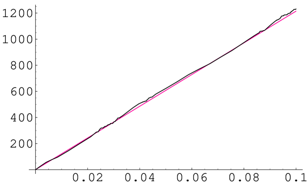
Figure 2: The number of vacua ${\cal N}(-F,F)$ plotted against $F$. The actual distribution for our example with $N=15$ is the bumpy line, compared with the statistical expectation

Figure 3: Closeup of the distribution–we see that the smallest $F$ is indeed of order $2^{-15}$.

2.1.2 (Non)-scanning of couplings

We are now in a position to ask whether the presence of the huge $2^{N}$ number of vacua guarantees that we will be able to find one with small enough vacuum energy. Interestingly, the answer is no. To see why, let us examine the distribution for the vacuum energy

$$\rho(\Lambda)=\frac{2^{N}}{\sqrt{2\pi N}V_{{\rm dif}}}\,e^{-\frac{(\Lambda-N\bar{V}_{{\rm av}})^{2}}{2NV^{2}_{{\rm dif}}}}$$ (21)

This distribution densely scans a region of width $\sim\sqrt{N}V_{{\rm dif}}$ around a central value $\sim NV_{{\rm av}}$. This would guarantee that we could find a tiny vacuum energy of order $\sim M_{*}^{4}2^{-N}$, for $\bar{V}_{\rm av}$ of order $\sim 1/\sqrt{N}M_{*}^{4}$. But what should we expect for $\bar{V}_{{\rm av}}$? Unfortunately in a non-supersymmetric theory, the vacuum energy is UV sensitive and not calculable. However, we have $N$ non-supersymmetric sectors, each of which contributes at least an amount $\sim M_{*}^{4}$ to the vacuum energy, so it is reasonable to expect that

$$N\bar{V}_{\rm av}=\bar{\Lambda}\sim NM_{*}^{4}$$ (22)

and so $\bar{V}_{{\rm av}}\sim M_{*}^{4}$. One might naively think that the signs of the vacuum energy randomly vary from sector to sector, so that the sum of vacuum energies fluctuates around zero, and $\bar{\Lambda}$ is of order $\sqrt{N}$ rather than $N$. However, in a non-supersymmetric theory, there is nothing special about zero vacuum energy, so there is no reason to expect the vacuum energy to scan around zero. For instance, the zero-point energy of the $N$ scalars is $\sim NM_{*}^{4}$, so that is where one should expect the mean vacuum energy to lie; a much smaller value would require a tuning. If $\bar{\Lambda}$ has its natural value near $\sim NM_{*}^{4}$, then in the central region of the Gaussian distribution, values of the vacuum energy with $\Lambda=\bar{\Lambda}\pm\delta\Lambda$ are finely scanned, with

$$\delta\Lambda/\bar{\Lambda}\sim\frac{1}{\sqrt{N}}$$ (23)

In particular, this tells us that we don’t get to scan around zero vacuum energy in the central region of the Gaussian.

This small width for the scanned region for the vacuum energy has a purely statistical origin; the actual width of the scanned region can be even further suppressed by weak coupling factors. Let us suppose that the quartic coupling for our scalars $\phi$ is perturbative $\sim g^{2}$, and all the other couplings in the theory are included with their natural sizes. Note that $V_{dif}$ vanishes in the limit where the cubic and linear couplings vanish, so we include these with their largest natural sizes; the potential $V(\phi)$ is then of the form

$$V(\phi)=g^{2}\left(\phi^{4}+\epsilon M_{*}\phi^{3}+\epsilon^{2}M_{*}^{2}\phi^{2}+\epsilon^{3}M_{*}^{3}\phi\right)$$ (24)

where $\epsilon^{2}\sim 1/(16\pi^{2})$ is a loop factor. The vevs of $\phi$ are then of order $\langle\phi\rangle\sim\epsilon M_{*}$, so

$$V_{{\rm dif}}\sim g^{2}\epsilon^{4}M_{*}^{4}$$ (25)

and the tunneling rate for the false vacuum can easily be seen to be of order

$$\Gamma\sim M_{*}^{4}e^{-c\frac{27\pi^{2}}{g^{2}}}$$ (26)

where $c$ is an ${\cal O}(1)$ factor. Thus we need to be parametrically at weak coupling, with small $g^{2}/16\pi^{2}$, to have a long-lived enough vacuum. In this model, $\delta\Lambda\sim\sqrt{N}V_{{\rm dif}}\sim\sqrt{N}g^{2}\epsilon^{4}M_{*}^{4}$, while $\bar{\Lambda}\sim N\epsilon^{2}M_{*}^{4}$, and

$$\delta\Lambda/\bar{\Lambda}\sim\frac{g^{2}}{16\pi^{2}}\frac{1}{\sqrt{N}}$$ (27)

so as promised, we see that, in addition to the statistical $1/\sqrt{N}$ suppression of the scanning for the vacuum energy, there is also a weak-coupling suppression by $\sim g^{2}/16\pi^{2}$, which is tied to the longevity of the false vacuum in this model.

While for natural values of $\bar{\Lambda}$, the large number $2^{N}$ of vacua does not in itself guarantee the presence of a vacuum with tiny vacuum energy in the fat region of the Gaussian distribution, it may be possible to find one on the tail of the Gaussian, since

$$\rho(\Lambda\sim 0)\sim\frac{1}{V_{{\rm dif}}}\times\left(2\,e^{-\frac{\bar{V}_{{\rm av}}^{2}}{V_{{\rm dif}}^{2}}}\right)^{N}$$ (28)

Therefore if

$$\frac{\bar{V}_{{\rm av}}^{2}}{V_{{\rm dif}}^{2}}<{\rm log}~{}2$$ (29)

we can still find a tiny vacuum energy at large $N$. However, this is condition may be difficult to satisfy; for instance, in our weakly coupled coupled model,

$$\frac{\bar{V}_{av}^{2}}{V_{{\rm dif}}^{2}}\sim\frac{16\pi^{2}}{g^{2}}\gg{\rm log}2$$ (30)

We have come to an interesting conclusion. In order for our landscape to solve the cosmological constant problem, in addition to the exponentially large number of vacua, we require an extra accident! Either a tiny CC can arise on the tail of a Gaussian distribution, or more likely, an extra accidental fine-tuning is required for the central value of $\bar{\Lambda}$ to be of order $\sim\sqrt{N}M_{*}^{4}$ rather than $\sim NM_{*}^{4}$.

However, if this accident did not happen, our landscape would not lead to a meaningful low-energy effective theory. One might imagine that, in a larger “global” picture of the landscape, in most regions $\Lambda$ never gets scanned enough to find a small enough expansion rate for the universe to allow the formation of structure, but that in $\sim 1/\sqrt{N}\sim$ a few percent of the regions, the required accident occurs and leads to a low-energy effective theory with a finely scanned $\Lambda$. Also, as we will see, in supersymmetric theories the situation is better–the combination of SUSY together with unbroken (discrete) R symmetries can guarantee that the distributions are peaked around $\Lambda=0$.

2.1.3 Coupling to the Standard Model

We can now imagine coupling the landscape fields to the Standard Model. At the renormalizable level, the only allowed couplings are of the form

$$\mu\phi h^{\dagger}h,\lambda\phi^{2}h^{\dagger}h$$ (31)

which would suggest that, together with the vacuum energy, the Higgs mass is scanned from vacuum to vacuum (actually, integrating out the heavy $\phi$ excitations around the vacua at tree-level also generates a Higgs quartic that varies). This would be the case if the vevs $\langle\phi\rangle$ are much smaller than the cutoff $M_{*}$ of the theory, but in our non-supersymmetric examples this is not natural. We can’t neglect higher-dimension operators, which are an expansion in powers of $(\phi/M_{*})$, so that the Lagrangian takes the form

$${\cal L} = -\left(g_{0}^{-2}+\sum_{i}g_{i}^{-2}(\frac{\phi_{i}}{M_{*}})\right)F_{\mu\nu}^{2}+\left(Z_{0\psi}+\sum_{i}Z_{\psi i}(\frac{\phi_{i}}{M_{*}})\right)\bar{\psi}\bar{\sigma}D\psi$$ (32)

$$+ \left(Z_{h0}+\sum_{i}Z_{hi}(\frac{\phi}{M_{*}})\right)|Dh|^{2}-\left(m_{0}^{2}+m^{2}_{i}(\frac{\phi_{i}}{M_{*}})\right)|h|^{2}-\left(\lambda_{0}+\sum_{i}\lambda_{i}(\frac{\phi_{i}}{M_{*}})|h|^{4}\right)$$

$$+ \left(\lambda_{0ab}+\sum_{i}\lambda_{abi}(\frac{\phi_{i}}{M_{*}})\right)\psi_{a}^{c}\psi_{b}h+\cdots$$

The notation is self-explanatory. For the case of the Yukawa couplings, we will assume for now that the $\phi$’s are not charged under any of the approximate chiral symmetries of the SM fermions, so that whatever explains the Yukawa hierarchies and suppresses the $\lambda_{0ab}$ (via flavor symmetries, separation in extra dimensions, or whatever else) also similarly suppresses $\lambda_{abi}$.

Note that we have again assumed that there are no cross-couplings in the interactions of the SM with the landscape fields. As in the case with the vacuum energy in the last subsection, some such couplings are inevitably induced by loops of gravity, and now also loops of SM fields. But just as before, the cross-couplings are parametrically suppressed at large $N$ and can be neglected.

In this non-supersymmetric example, the vevs $\langle\phi_{i}\rangle$ will be close to $M_{*}$, and the suppression of higher dimension operators is not significant, so all the couplings can in principle scan in the landscape. Actually, if the theory is weakly coupled with a weak coupling factor $\sim g^{2}$, the expansion in higher dimension operators is really in the combination $(g\phi)/M_{*}$, so that the higher dimension operators will indeed be suppressed. However, as we have already seen for the vacuum energy, even discounting any weak coupling factors, the variation in any coupling $c$ is generally small for purely statistical reasons

$$\delta c/\bar{c}\lower 3.01385pt\hbox{$\;\stackrel{{\scriptstyle\textstyle<}}{{\sim}}\;$}\frac{1}{\sqrt{N}}$$ (33)

The reason is just as for the vacuum energy. The value of a coupling $c$ for any given vacuum $\{\eta\}$ is of the form

$$c_{\{\eta\}}=c_{0}+\sum_{i}c_{{\rm av}i}+\sum_{i}\eta_{i}c_{{\rm difi}}$$ (34)

which are significantly scanned in the landscape in a region

$$c_{0}+N\bar{c}_{{\rm av}}\pm\sqrt{N}c_{{\rm dif}}$$ (35)

Now, the magnitude of the variation of couplings depends upon how the couplings $c_{i}(\phi_{i}/M_{*})$ to the landscape fields are scaled at large $N$. If the scaling is chosen so that the large $N$ limit has fixed coupling strengths, then $N\bar{c}_{{\rm av}}$ is subdominant to $c_{0}$, and

$$\delta c/\bar{c}\ll\frac{1}{\sqrt{N}}$$ (36)

On the other hand, if the $N\bar{c}_{{\rm av}}$ term dominates $c_{0}$, then we have the largest scanning region, which is still suppressed at large $N$

$$\delta c/\bar{c}\sim\frac{1}{\sqrt{N}}$$ (37)

2.1.4 Origin of weak couplings $\alpha\sim 4\pi/N$

It is interesting to consider this last limit in more detail. Suppose that the theory is intrinsically strongly coupled at the scale $M_{*}$. From naive dimensional analysis [38], we expect that the effective Lagrangian takes the form

$${\cal L}=\frac{1}{16\pi^{2}}\left(\sum_{i}f_{i}(\frac{\phi_{i}}{M_{*}})F_{\mu\nu}^{2}+\cdots\right)$$ (38)

where all the $f_{i}$ are of ${\cal O}(1)$. Then, since each of the terms in the sum is of ${\cal O}(1)$, the Lagrangian in any of the densely scanned vacua takes the form

$$\sim\frac{N}{16\pi^{2}}\left((1\pm{\cal O}(1/\sqrt{N}))F_{\mu\nu}^{2}+\cdots\right)$$ (39)

(Here again, the fact that there is nothing special about zero tells us that the expected coefficient is of order $N$, not $\sqrt{N}$). This means that all the dimensionless couplings in the theory are weak

$$\frac{1}{g^{2}}\sim\frac{N}{16\pi^{2}}\to\frac{g^{2}}{16\pi^{2}}\sim\frac{1}{N}$$ (40)

and of course none of them scan significantly

$$\delta g/g\sim\frac{1}{\sqrt{N}}$$ (41)

This can provide an attractive explanation for the relative weakness of the SM couplings, with $\alpha\sim 4\pi/N$.

2.2 General lessons

We have seen that, in our landscape of vacua, despite the presence of a huge number $2^{N}$ of vacua, the most natural situation is that none of the couplings are effectively scanned from vacuum to vacuum. This is because while the scanning allows us to sample a region of size proportional to $\sqrt{N}$ around a mean, the mean coupling induced from interactions with $N$ landscape fields will itself be proportional to $N$, so that the relative deviations from central values are down by (at least) ${\cal O}(1/\sqrt{N})$.

Figure 4: Generic scanning of couplings on our landscape. Note that the region of the scanned couplings is small, $\delta c/c\lower 3.01385pt\hbox{$\;\stackrel{{\scriptstyle\textstyle<}}{{\sim}}\;$}1/\sqrt{N}$, since the mean value of the coupling grows as $N$ while the width only grows as $\sqrt{N}$

This conclusion can be avoided if, for some symmetry reason, the central value of the coupling $\bar{c}_{av}$ vanishes. In this case, a region of size $\sqrt{N}c_{{\rm dif}}$ is efficiently scanned.

Figure 5: If for a symmetry reason, the mean value of the coupling vanishes, the scanning can be efficient.

However, in our non-supersymmetric examples, there are no symmetries that can guarantee $\bar{c}_{{\rm av}}=0$. Even the $\phi\to-\phi$ symmetry is necessarily broken in order to have $V_{{\rm dif}}\neq 0$, required to be able to scan the vacuum energy.

This means that, naturally, none of the couplings vary significantly in the landscape, unless for an accidental reason, the central values are of order $\sqrt{N}$ rather than $N$. This would take an accident or tuning of order $1/\sqrt{N}$. But this accident must happen for the relevant operators in theory, such as the cosmological constant and the Higgs mass. If not, there would not be any low-energy effective theory to speak of: if the CC doesn’t scan, all the vacua have curvatures near the fundamental scale, and if the Higgs mass doesn’t scan, there is no Higgs field in the low-energy effective theory. In this sense, the relevant operators are special, since they have the largest impact on the IR physics. But there is no worry about all parameters varying wildly on the landscape–on the contrary they naturally don’t vary significantly at all.

We have therefore provided a rationale for the existence of a “friendly neighborhood” of the landscape, where the only couplings that are scanned are relevant operators, while the dimensionless couplings are essentially fixed. If our low-energy model for the landscape could be derived from a UV complete theory, despite the enormous number of vacua in the effective theory, all the dimensionless parameters could be predicted to ${\cal O}(1/\sqrt{N})\sim$ 5 $\%$ accuracy each! And while the relevant couplings scan and therefore take widely differing values across vacua, being relevant, they have the largest impact on IR physics, and therefore very gross environmental arguments (such as the existence of structure or atoms) can be used to fix their values as well.

The theories where the large $N$ number of fields lead to weak Standard Model couplings with $\alpha\sim 4\pi/N$ are particularly attractive, since in these cases, all hierarchies in nature can be seen to be exponentially large in $N$. This is because the asymptotically free couplings generate exponentially low scales $\Lambda_{IR}\sim e^{-8\pi^{2}/bg^{2}}\sim e^{-cN}$, and while the relevant couplings are not determined, environmental arguments peg their values to various powers of the scales $\Lambda_{IR}$. Thus for instance, the “atomic” principle fixes the weak scale (and thus the Higgs mass squared parameter) to $\Lambda_{QCD}$, while Weinberg’s argument pegs $\Lambda^{1/4}\sim m_{DM}^{2}/M_{Pl}$, and the $m_{DM}$ scale can be determined by dimensional transmutation. Even in a theory without DM, Weinberg’s argument would have set $\Lambda^{1/4}\sim\eta_{B}\Lambda_{QCD}$. Thus, in this picture of the world, all hierarchies are determined first through dynamics (via dimensional transmutation of marginal couplings) and then by environmental arguments (for the relevant couplings) to be of the form $e^{-cN}$ for various $O(1)$ parameters $c$.

2.3 Supersymmetric Landscapes

We can also build supersymmetric landscapes. This gives an immediate advantage–what were UV sensitive relevant operators in the SM, such as the cosmological constant and the Higgs mass, are UV insensitive in supersymmetric theories, so our distributions for the CC and scalar masses will be calculable.

In analogy with our non-SUSY example, suppose we have a chiral superfield with a general cubic superpotential

$$W=m^{2}\phi+\mu\phi^{2}+\lambda\phi^{3}$$ (42)

where we take $m\sim\mu$ near the cutoff scale $M_{*}$. There are two supersymmetric minima at $\langle\phi\rangle=\phi_{\pm}$, and at these two minima, there are in general two different vevs for the superpotential $\langle W\rangle=W_{\pm}$. Once again imagine we have $N$ decoupled sectors of this type, so there are $2^{N}$ supersymmetric minima labeled by $\{\eta\}$. The value of the superpotential in these minima is

$$W_{\{\eta\}}=\sum_{j}W_{j}=N\bar{W}_{{\rm av}}+\sum_{i}\eta_{i}W_{{\rm dif}i}$$ (43)

As in the previous section, we will now have a distribution of possible $W$’s, peaked around $NW_{{\rm av}}$ with a width of order $\sqrt{N}W_{{\rm dif}}$. When we turn on gravity, each of these become AdS minima, with vacuum energy $-3|W|^{2}/M_{Pl}^{2}$ distributed around $-3|NW_{{\rm av}}|^{2}/M_{Pl}^{2}$.

Suppose now that SUSY is broken in a hidden sector, at a scale $\Lambda_{S}$, parametrically smaller than $M_{*}$, contributing a positive vacuum energy $\sim\Lambda_{S}^{4}$. Again, for the most natural value of $W_{{\rm av}}\sim M_{*}^{3}$, it is not possible to cancel this positive energy from the $-3|W|^{2}/M_{Pl}^{2}$ AdS vacuum energies.

However, in this supersymmetric theory, there is a symmetry that can enforce $\bar{W}_{{\rm av}}=0$. Suppose that the superpotential is an odd polynomial in $\phi$, e.g.

$$W=\lambda\phi^{3}-\mu^{2}\phi$$ (44)

This form can be enforced by a discrete $Z_{4}$ R symmetry under which $\phi(y,\theta)\to-\phi(y,i\theta)$. In this case, $W_{+}=-W_{-}$, so that $W_{{\rm av}}=0$. Then, the landscape sector scans vacuum energies in the range

$$0\geq\Lambda_{{\rm landscape}}\lower 3.01385pt\hbox{$\;\stackrel{{\scriptstyle\textstyle>}}{{\sim}}\;$}-3\frac{|\sqrt{N}W_{{\rm dif}}|^{2}}{M_{{\rm Pl}}^{2}}$$ (45)

so that it is always possible to find a vacuum that cancels the $+\Lambda_{S}^{4}$ vacuum energy from SUSY breaking, to an accuracy of order $\sim 2^{-N}M_{*}^{4}$.

Depending on how this landscape sector couples to the Standard Model fields, we can arrive at a variety of low-energy theories.

2.3.1 MSSM scanning only $\Lambda$

The most straightforward possibility is that the landscape sector does not couple to the MSSM, or that, as in our non-SUSY examples, there is a coupling, but none of the MSSM couplings scan effectively in the landscape. In this case, the only coupling that does scan effectively is the cosmological constant. Thus, this is a landscape that gives us the conventional supersymmetric standard model at low-energies, with the landscape only playing a role in solving the cosmological constant problem.

2.3.2 The $\mu$ and doublet-triplet splitting problem

Another interesting possibility arises if we recall that there is another natural parameter in the MSSM that can be set to zero by symmetry arguments: the $\mu$ term $\mu H_{u}H_{d}$ in the superpotential. In fact, we can use exactly the same $Z_{4}$ R symmetry as before, with the $H_{u,d}$ carrying R charge $0$ and the SM matter fields carrying $R$ charge 1, to forbid a $\mu$ term. However, we can have couplings of the form

$$\sum_{i}g_{i}M_{*}P_{i}(\phi_{i}/M_{*})H_{u}H_{d}$$ (46)

where $P_{i}$ is any odd polynomial in $\phi_{i}$. In turn, this leads to the $\mu$ term being scanned about a zero central value on the landscape. Note that the discrete $R$ symmetry forces the Yukawa couplings to be of the form

$$\sum_{i}\lambda_{abi}(\phi_{i}/M_{*})f_{a}f_{b}^{c}H$$ (47)

where the $\lambda_{abi}$ are even in $\phi$, so they are not effectively scanned in the landscape.

Therefore in this landscape, it is the CC and $\mu$ term that are scanned, while all other parameters (including dimensionless couplings and SUSY breaking soft terms) are fixed. This can in turn lead to an environmental solution to the $\mu$ problem, if we use the atomic principle to fix the Higgs VEV, which is applicable independent of the mechanism of SUSY breaking (gravity, gauge etc. mediation), and does not require the presence of any light particles. This is especially interesting if the landscape favors very low energy scales of SUSY breaking, e.g. gauge mediated SUSY breaking, as in these theories the $\mu$ problem is challenging and typically requires excessively clever model-building gymnastics and a rich spectrum of new light particles. In grand unified theories this mechanism evolves into a solution of the closely related doublet-triplet splitting problem [2]. In minimal SU(5), for example, the superpotential

$$W=H_{u}\,\left(M+\langle\Sigma\rangle\right)\,H_{d}$$ (48)

responsible for the Higgs doublet and (SU(3)) triplet masses (where $\langle\Sigma\rangle$ is the adjoint VEV $\sim M_{GUT}\sim 10^{16}$ GeV ) typically gives a mass of order $\sim M_{GUT}$ to both the doublets and triplets. With $M$ scanned, only where $M$ and $\langle\Sigma\rangle$ almost cancel—to give a small $\mu$ term for the doublets— is the electroweak VEV near its experimental value, as required by the atomic principle.

2.3.3 The Standard Model, scanning only $\Lambda$ and $m_{h}^{2}$

Suppose that the SUSY breaking masses in the MSSM, $\tilde{m}\sim F_{Z}/M_{*}$, are much much higher than the TeV scale, but still small compared with the scale $M_{*}$. What does the effective theory look like at energies far lower than $\tilde{m}$? Of course, in most of the landscape, all the scalars (including both Higgses) as well as the gauginos will be near $\tilde{m}$. Since the $\mu$ term for the Higgs is scanned, it is possible to find Higgsinos surviving beneath $\tilde{m}$. However, there is a different part of the landscape, where the squarks, sleptons and gauginos are heavy, but a single linear combination of the Higgses can be light. Recall that the Higgs mass matrix is of the form

$$\pmatrix{\tilde{m}_{u}^{2}+\mu^{2}&\tilde{m}^{2}_{ud}+B\mu\cr B\mu+\tilde{m}^{2}_{ud}&\tilde{m}_{d}^{2}+\mu^{2}}$$ (49)

As mentioned, $\tilde{m}^{2}_{u,d,ud}$ and $B$ do not vary in the landscape, while $\mu$ is scanned. Note that the sum of the eigenvalues of the $m^{2}$ matrix is

$$m_{1}^{2}+m_{2}^{2}=\tilde{m}_{u}^{2}+\tilde{m}_{d}^{2}+2\mu^{2}>\tilde{m}_{u}^{2}+\tilde{m}_{d}^{2}$$ (50)

and if $\tilde{m}_{u}^{2}+\tilde{m}_{d}^{2}>0$, then at least one of the eigenvalues of $m^{2}$ must be comparable to $\tilde{m}^{2}$. However, as $\mu$ varies in the landscape, it is possible that one of the eigenvalues is fine-tuned to be light. Note that clearly this can only happen in the region of the landscape where $\mu\sim\tilde{m}$, and that in this region the Higgsinos are heavy, also at $\tilde{m}$. At low-energies, we have the Standard Model with a single Higgs doublet. The value of $\mu$ where the SM Higgs is light can be found just by setting the determinant of the mass matrix to zero. This fixes $\mu$ and also the linear combination of $h_{u,d}$ that is tuned to be light

$$h=\mbox{cos}\beta h_{u}+\mbox{sin}\beta h_{d}$$ (51)

Note that as $\mu$ is then scanned in this vicinity, $m_{h}^{2}$ is clearly scanned, but tan$\beta$ remains fixed to an accuracy of $O(\sim m_{h}^{2}/\tilde{m}^{2})$.

We have thus found an example of a SUSY landscape that reduces to the Standard Model at energies far below a (very high) SUSY breaking scale $\tilde{m}$, and where a discrete symmetry guarantees that the vacuum energy and Higgs mass are finely scanned, while all other parameters are effectively fixed.

2.3.4 Scanning SUSY breaking scales

In our discussion so far, we imagined that the SUSY breaking scale was not scanned in the landscape. It is also instructive to consider theories where the SUSY breaking sector couples to the landscape. Consider a chiral superfield $X$, with a coupling to the landscape sector of the form

$$W_{X}=\sum_{i}M_{*}^{2}\lambda_{i}P_{i}(\phi_{i}/M_{*})X$$ (52)

where again the $Z_{4}$ R symmetry guarantees $P_{i}$ is an odd polynomial in $\phi_{i}$. Integrating out the heavy $\phi$’s would generate a superpotential for $X$ of the schematic form

$$M_{*}^{2}(\lambda X)+M_{*}(\lambda X)^{2}+(\lambda X)^{3}+\cdots$$ (53)

which clearly has stationary points for

$$X\sim\frac{M_{*}}{\lambda}$$ (54)

However, higher order terms in the Kahler potential for $X$

$$\int d^{4}\theta-\frac{X^{2}X^{\dagger}}{M_{*}}+\mbox{h.c.}+\cdots$$ (55)

can lead to a local minimum with broken SUSY, with SUSY broken by non-vanishing $F_{X}$. Because of the $Z_{4}$ R symmetry, $F_{X}$ will vary around a mean of zero,

$$\frac{F_{X}}{M_{*}^{2}}=\sum_{i}\eta_{i}P_{{\rm dif}\,i}$$ (56)

and will scan effectively in the landscape. Since the distributions of $F_{X}$ and $W$ are independent, the tuning required to cancel the CC is independent of the actual value of the SUSY breaking scale.

If we concentrate on the vacua with tiny vacuum energy, the physical measure of SUSY breaking is the gravitino mass

$$m_{3/2}^{2}=\frac{|F_{X}|^{2}}{M_{Pl}^{2}}=\frac{({\rm Re}F_{X})^{2}+({\rm Im}F_{X})^{2}}{M_{Pl}^{2}}$$ (57)

Both Re$(F_{X})$ and Im $(F_{X})$ have approximately flat distributions around $0$. In turn, this implies that the density of distribution for $m_{3/2}$ is proportional to $m_{3/2}$

$$\rho(m_{3/2})\propto m_{3/2}$$ (58)

That is, there are more vacua with ${\it high}$ scale SUSY breaking in this theory. Note that if for some reason, all the $F_{X}$ in the distribution had the same phase (say because of a conserved $CP$ symmetry), we would instead have $\rho(m_{3/2})\propto 1$. We can also generalize to having $n$ fields $X_{a}$, $a=1,\cdots,n$ that break SUSY. Then, each of the Re($F_{X_{a}}$), Im($F_{X_{a}}$) have a flat distribution, but

$$m_{3/2}^{2}=\frac{\sum_{a}|F_{X_{a}}|^{2}}{M_{Pl}^{2}}$$ (59)

has a distribution

$$\rho(m_{3/2})\propto(m_{3/2})^{2n-1}$$ (60)

Now, suppose the scalars of the MSSM also pick up a mass of order $\tilde{m}^{2}\sim m_{3/2}^{2}$ from gravity-mediated SUSY breaking. In what fraction of vacua do we expect to have a Higgs mass of $\sim m_{h}^{2}$? For a given $\tilde{m}^{2}>m_{h}^{2}$, there is a tuning of magnitude $\sim(m_{h}^{2}/\tilde{m}^{2})$ required to keep the Higgs light. However, for $n>1$, there are many more vacua with large SUSY breaking scales, and the number of vacua with SUSY broken at the scale $\sim\tilde{m}$ is proportional to

$$\left(\frac{m_{h}^{2}}{\tilde{m}^{2}}\right)\times\left(\frac{\tilde{m}^{2}}{M_{*}^{2}}\right)^{2n-1}$$ (61)

Thus, there are more vacua with a given value of the weak scale, with SUSY broken at high scales than at low scales. The fact that the distribution of $F$ and $D$ terms, if sufficiently uniform, will statistically favor high scale SUSY breaking on the landscape has been discussed in the context of stringy constructions in [39, 40, 41, 42]. It is even plausible that KK scale breaking will be favored in this sense [43].

2.3.5 A Landscape for split SUSY

We can also build a landscape realizing the scenario of split SUSY. In one limit of split SUSY, the scalars are only at about $\sim 100-1000$ TeV. This can arise from conventional hidden sector SUSY breaking if there are no singlets in the hidden sector. While the scalars can pick up a mass from operators suppressed by $M_{*}\sim M_{GUT}$, so that $\tilde{m}\sim F/M_{*}$, the gauginos pick up a mass $\sim\alpha/\pi m_{3/2}$ from anomaly mediation [44], where $m_{3/2}\sim F/M_{Pl}$. So, we can have $\tilde{m}\sim 1000$ TeV, $m_{3/2}\sim 30$ TeV and the remaining fermions near the $\sim$ TeV scale. This scenario is very plausible. We can realize it on the landscape in the same way as our model above, which reduced to the SM with a tuned Higgs mass at low energies.

But we can also consider the more extreme version of split SUSY, with the scalars and gravitino being very heavy. To do this, we want to break SUSY without breaking R symmetry.

Fortunately, the classic model of SUSY breaking–the O’Raigheartaigh theory, is precisely an example of a theory that breaks SUSY while preserving $R$. Consider the theory with three chiral superfields $X,Y,Z$ and superpotential

$$\lambda Y(Z^{2}-\mu^{2})+mZX$$ (62)

This model has an $R$ symmetry under which $Y,X$ have charge 2 while $Z$ has charge 0. It is simple to understand the physics in the limit where $m<\lambda\mu$. The $Y$ equation of motion forces $Z$ to get a vev; there are two vacua with $Z=\pm\mu$. In these vacua, $Y,Z$ marry up to get a mass $\mu$. Integrating out the heavy fields leaves us with the superpotential

$$W=m\mu X$$ (63)

while at 1-loop, we generate a correction to the Kahler potential of $X$ as

$$\Delta K=-\frac{1}{24\pi^{2}}\left|\frac{\lambda m}{\mu}\right|^{4}\frac{(X^{\dagger}X)^{2}}{|\mu|^{2}}$$ (64)

This breaks SUSY with $F_{X}=m\mu\neq 0$, while the induced term in the Kahler potential stabilizes the modulus $X$ around $X=0$ with the correct sign so that $m_{X}^{2}>0$. Thus, SUSY is broken while $R$ is preserved.

It is a simple matter to extend this picture to a landscape. We take $N$ copies of $Y,Z$ as

$$W=\lambda_{j}Y_{j}(Z_{j}^{2}-\mu_{j}^{2})+m_{j}Z_{j}X$$ (65)

This form of the superpotential can be guaranteed by $R$ symmetries and a discrete $Z_{2}$ symmetry under which $Z_{j}$ and $X$ change sign.

Once again, there are $2^{N}$ vacua. In each of these vacua, SUSY is broken and $R$ symmetry is preserved, and

$$F_{X}=m_{j}\langle Z_{j}\rangle$$ (66)

Note that $F_{X}$ is scanned around a mean value $F_{X{\rm av}}=0$ with a width of order $\sim\sqrt{N}M_{*}^{2}$; this is guaranteed by the $Z_{2}$ symmetry. In this model, it is therefore positive vacuum energies $\Lambda=|F_{X}|^{2}$ that are scanned in the landscape over a range

$$NM_{*}^{4}\lower 3.01385pt\hbox{$\;\stackrel{{\scriptstyle\textstyle>}}{{\sim}}\;$}\Lambda\geq 0$$ (67)

Now, in order to find a vacuum with small cosmological constant, we need to have a non-zero vev of the superpotential, which requires a source of $R$-breaking. Suppose that there is a sector with pure SUSY Yang-Mills with dynamical scale $\Lambda_{{\rm strong}}$, giving rise to gaugino condensation with

$$\langle W\rangle=\Lambda_{{\rm strong}}^{3}$$ (68)

Recall that the gauge couplings and hence $\Lambda_{{\rm strong}}$ do not scan significantly in the landscape. If we have many groups with gaugino condensation, we will get the sum of $\Lambda_{{\rm strong}}^{3}$ from each sector, and $W$ will be dominated by the largest $\Lambda_{{\rm max}}$.

Therefore, while the distribution for $F_{X}$ does not favor either low or high energy SUSY breaking, the requirement of cancelling the cosmological constant fixes the SUSY breaking scale to be

$$|F_{X}|\sim\frac{\Lambda_{{\rm max}}^{3}}{M_{Pl}}$$ (69)

We stress that this is not simply a purely statistical question about there being more or less vacua with a given scale of SUSY breaking and vanishing vacuum energy–it is only possible to cancel the vacuum energy for a fixed value of SUSY breaking scale. If $\Lambda_{{\rm max}}$ is relatively high, this will force (rather than merely statistically favor) high-energy SUSY breaking. This landscape illustrates one of the motivations for split SUSY given in [33]. There may be regions of the landscape with SUSY broken at low energies, and others with SUSY broken at high energies. The latter may naively be disfavored because of the additional tuning required for the hierarchy problem. But, it may be that it is impossible to cancel the cosmological constant in theories with a conventional low breaking scale for SUSY. We see this explicitly in our example.

Since the high-scale breaking of SUSY preserves $R$-symmetry, we are naturally let to a prediction of split SUSY at low energies [33, 35]. Of course, we must also be able to scan for the Higgs mass. Interestingly, in our landscape, of all the scalars of the MSSM, only a single Higgs doublet can be fine-tuned to be light. Note that the $R$-symmetry forbids any $\mu$ term for the Higgsinos; however, a $B$-term of the form

$$\int d^{2}\theta b_{j}\frac{Z_{j}X}{M_{*}}H_{u}H_{d}$$ (70)

is allowed, and scans around $0$ in the landscape. Meanwhile, the soft masses for all the scalars are essentially fixed. This means that none of the squarks or sleptons can become light. But the Higgs mass matrix is

$$\pmatrix{\tilde{m}_{u}^{2}&\mu B\cr\mu B&\tilde{m}_{d}^{2}}$$ (71)

which can have a single small eigenvalue over the appropriate range of $\mu B$’s.

Thus, we have SUSY broken at a very high energy scale, with all scalars heavy and a single finely tuned Higgs light, and light Higgsinos and gauginos. Of course, the inevitable breaking of R by $\langle W\rangle$ eventually generates $R$-breaking fermion mass terms, leading to light but not massless Higgsinos and gauginos. As discussed in [33, 35], this can in fact naturally lead to gauginos and Higgsinos near the $\sim 100$ GeV scale.

2.4 Relation to the string theory landscape

The motivation for the idea that we live in a “friendly neighborhood” of the landscape, where only the dimensionful (relevant) couplings of the theory are finely scanned from vacuum to vacuum, comes entirely from data via Weinberg’s prediction of the cosmological constant. Our simple field theory examples above illustrate what such a landscape might look like. These models are meant to only describe a “local” region of the landscape where things like spacetime dimensionality, low-energy gauge symmetry, particle content and so on are fixed. There is of course a much larger “global” landscape, where all of these things can change. It is important to stress that are also other “local” landscapes where “friendliness” is not guaranteed in the same way. Let us call the landscapes we have studied $2^{N}$ landscapes for obvious reasons. Some of the conclusions which follow from basic statistics applied to the $2^{N}$ ensemble, do not apply to slightly more complicated (but still well-motivated) ensembles. The best studied case in string theory so far, is the ensemble of type IIB Calabi-Yau flux vacua, which exhibits some differences.

As we have emphasized, one of the main features of the $2^{N}$ landscapes is that one finds that scanning of couplings is difficult. In particular, we find Gaussian distributions which make it difficult to scan even small vacuum energy, under some assumptions; or in SUSY theories, a Gaussian distribution of $W$ values.

In the IIB flux ensemble, the distributions of $W$ values and vacuum energies (under suitable assumptions, but really governed by periods of the Calabi-Yau compactifications) have also been studied in some detail now [16, 23]. The results are somewhat different – for instance, $W$ does not have a Gaussian distribution, and scanning a large range of values is not difficult, even without the microscopic imposition of an R-symmetry. This is certainly not a contradiction since the ensemble involves more complicated interactions between the fields – the periods are generally complicated transcendental functions of the moduli, and hence a distribution governed by randomly selected flux potentials need not behave like the $2^{N}$ ensemble.

However, this illustrates that even very basic results for vacuum distributions may vary in different plausible ensembles. In non-supersymmetric $2^{N}$ ensembles, nothing is efficiently scanned. The minimal assumption that by luck $\Lambda$ can be scanned then leaves one in a friendly neighborhood. Or in SUSY examples with a discrete R symmetry on the landscape, the scanning of $\Lambda$ (and the Higgs mass) can be guaranteed by the discrete symmetry. In the IIB flux ensemble or other ensembles that are being investigated in various corners of string theory, the assumptions leading to friendliness may differ. It may be even easier to scan $\Lambda$ while other quantities don’t vary much; or maybe in some unusual cases it will be hard not to scan everything.

On the other hand, it is likely that ensembles similar to the $2^{N}$ ensembles are actually realized as part of the stringy landscape. For instance, one could presumably design flux potentials with properties similar to our $2^{N}$ models by choosing Calabi-Yau geometries with various discrete symmetries and local singularities, where the symmetries and locality forbid strong cross-coupling between the moduli related to different singularities. A wide class of effective field theories related to singularities in non-compact Calabi-Yau geometries, realizing rather general Landau-Ginzburg effective theories with many vacua (where the different vacua correspond to flux vacua realized with different flux choices), can be found in [45]. It would be interesting to demonstrate that brane constructions of the SM in these kinds of Calabi-Yau models [46], can be realized in a friendly neighborhood. One expects that varying fluxes far from the SM branes will scan over such a friendly neighborhood in many cases.

Summarizing, our main point is not that all regions of the landscape are indeed “friendly”. Rather, it is that data seems to point to such a neighborhood, and that it is simple to construct landscapes leading to friendliness. The non-trivial upshot of all of this is to suggest a new, predictive framework for thinking about physics beyond the standard model, which we turn to next.

3 Model-building rules in a predictive neighborhood

We have argued that we live in a friendly neighborhood of an enormous landscape of vacua, where only the relevant operators are finely scanned from vacuum to vacuum, while the dimensionless (nearly marginal) couplings are essentially fixed. This offers a highly restrictive and predictive new framework for model-building, where the finely tuned large hierarchies in nature are understood from environmental considerations associated with gross large-scale properties of the universe. These sorts of theories provide the first known framework in which to simultaneously address the cosmological constant problem together with the big and little hierarchy problems.

Indeed the most minimal model along these lines is the Standard Model itself, where the structure and atomic principles are used to explain the fine-tunings for the cosmological constant and the weak scale. As we have discussed above, note that one of the attractive aspects of our predictive neighborhood of the landscape is that, while there is no dynamical mechanism “stabilizing” large hierarchies, nonetheless the dimensionful quantities are environmentally predicted to be exponentially small compared to the cutoff, since they are inevitably pegged to other infrared scales generated by dimensional transmutation. For instance, the atomic principle sets the value of the weak scale to be close to $\Lambda_{\rm QCD}$, and the exponential smallness of $\Lambda_{\rm QCD}$ relative to the cutoff is understood via dimensional transmutation.

But there are reasons to suspect that there is new physics beyond the Standard Model near the TeV scale. Both the supersymmetric unification of gauge couplings and the success of stable weakly interacting stable TeV scale particles as dark matter candidates suggests that the Standard Model must be augmented at accessible energies. In the usual naturalness motivated theories of weak scale SUSY, these successes are gained, while the atomic principle explanation for the proximity of the weak to QCD scales is lost. Furthermore, as we have discussed, the “natural” theories all suffer from a little hierarchy problem–why haven’t we seen any indirect evidence for new physics? This has been a growing tension in beyond the standard model physics for the past two decades.

Split Supersymmetry offers a resolution to all of these puzzles. SUSY is broken at very high energies, with all the scalars becoming ultraheavy, except for single finely tuned Higgs that is forced to be light due to the atomic principle. Yet, the fermions of the MSSM are light, protected by an $R$ symmetry, and if they are near the TeV scale, account both for Dark Matter as well as the successful unification of gauge couplings. Since the only new particles beyond the Standard Model are fermions with only Yukawa couplings to the Higgs, there is an excellent reason why we have not seen any indirect effects associated with these particles. All of the dangerous operators in the MSSM are generated by light scalars in 1-loop diagrams, and disappear when the scalars are heavier than $\sim 1000$ TeV. The only remaining indirect processes arise at two loops with internal Higgs and new fermion lines; the most interesting of these is an electric dipole moment for fermions which is naturally just at the edge of planned new experiments [35].

Split SUSY is attractive for its conceptual simplicity, as well as a number of striking quantitative and qualitative predictions, which include a long-lived gluino, and supersymmetric unification at a single scale, of all 5 dimensionless parameters of the theory, leading to 4 predictions analogous to gauge coupling unification [35]. One drawback is that, there is no a priori reason to expect the gauginos and Higgsinos to be near the weak scale, although remarkably, in some models for SUSY breaking the $\sim 100$ GeV scale arose rather naturally for their masses. But there is no direct connection between the Dark Matter mass and the weak scale; the apparent proximity of these would then be an accident.

3.1 Minimal model for Dark Matter and Unification

It is interesting to ask whether there are even more minimal particle contents that give both a dark matter candidate and gauge coupling unification. In examining split SUSY itself, it is easy to see that at 1-loop the Higgsinos are most important for the relative running of the couplings. Let us therefore consider a model with only “Higgsinos” at the TeV scale (where now this is just a mnemonic for their quantum numbers since there is no longer a trace of SUSY at low energies). The neutral component of the Higgsinos can serve as a good dark matter candidate. We can also have additional singlet fermions in the theory, with Yukawa couplings to the “Higgsino”s and the Higgs. The DM particle can then be an admixture of the singlet and neutral Higgsino components.

Remarkably, in this minimal model, the standard model gauge couplings unify to high accuracy near $\sim 10^{14}$ GeV. While the 1-loop prediction for $\alpha_{s}(M_{Z})$ is lower than in the MSSM, two-loop running effects push up the predicted value for $\alpha_{s}$ to be about as far lower from central value as the MSSM prediction is higher. The two-loop running couplings $\alpha_{i}^{-1}$ are plotted below, with the Higgsinos put in at the mass of the top, and the 1-loop weak scale threshold corrections for the top and SM gauge bosons included in the usual way. We have not included the two-loop running contributions from the Higgsinos themselves, as these depend also on the Yukawa couplings to new singlet fermions. Nonetheless, we expect that a more complete analysis will confirm the basic result that gauge coupling unification works about as well as in the MSSM.

Figure 6: Two-loop gauge running of the couplings $\alpha_{i}^{-1}$ in the minimal model, as a function of log${}_{10}(E/$ GeV).

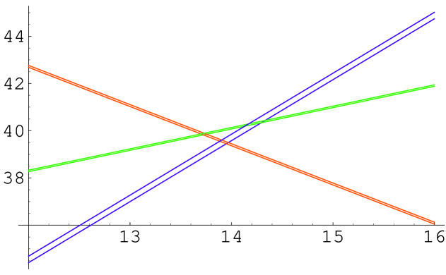
Figure 7: A close up of the running couplings near the unification scale

.

Since the unification scale is low, we can’t embed this theory into standard grand unified models like $SU(5)$ or $SO(10)$, because of gauge-mediated proton decay. However standard GUT’s suffer from problems of their own, such as doublet-triplet splitting, which are most naturally resolved in higher-dimensional [47](or deconstructed [48]) models with a GUT in the “bulk” and reduced gauge symmetry on the boundary. We can use exactly the same ideas in our case to dispense with proton decay from $X,Y$ gauge boson exchange. Indeed, having some of the extra dimensions in string theory stabilized to moderately large sizes $\sim 10-100$ times larger than the string scale can lower the string scale close to $\sim 10^{14}$ GeV, so it is natural to use these extra dimensions for GUT breaking. Furthermore, these theories induce calculable threshold corrections for the gauge couplings from running between the compactification scale and the unification scale, which are logarithmically enhanced relative the unknown UV threshold corrections. In the case of split SUSY, this has recently been studied [49], and it has been found that models with the Higgs doublets localized on a boundary further increase the low-energy prediction for $\alpha_{s}$; it would be interesting to redo this analysis for our model. If the third generation for the SM is placed in the bulk (or on a boundary with an unbroken GUT symmetry), we may preserve the success of $b/\tau$ unification [50], and also induce proton decay via CKM mixing–a simple estimate suggests that this gives a rate for proton decay on the edge of detection. A fundamental scale near $\sim 10^{14}$ GeV still allows us to use higher dimension operators for neutrino masses, and it is closer to the cosmologically allowed value of the axion decay constant $f\sim 10^{12}$ GeV so that a fundamental-scale axion can more easily solve the strong CP problem without having its coherent oscillations overdominate the universe.

3.2 New mechanisms for exponentially large hierarchies

Weinberg’s argument for the CC has a very satisfying binary character to it–either the CC is bigger than a critical value, and the universe is empty, or it is smaller, and the universe has structure. The atomic principle explanation of the hierarchy does not quite have the same character. However, our model-building rules suggest new solutions to the hierarchy problem using even more minimal environmental requirements than the existence of atoms, which share the “binary” feature of Weinberg’s argument: unless the Higgs mass is finely tuned to exponentially tiny values, an infrared disaster happens, such as a universe devoid of any structure or baryons.

We present below two models along these lines. Unlike split SUSY and the “only Higgsinos” model just discussed, these theories further predict that Dark Matter is at the weak scale. Furthermore, the minimal version of the second model we propose has the same SM charged particle content as the “only Higgsinos” model and therefore has gauge coupling unification to high accuracy near $\sim 10^{14}$ GeV.

3.2.1 Hierarchy from Structure

Consider a toy universe with a massive $U(1)$ gauge field, and a massive fermion, which consists of two Weyl spinors $\psi,\psi^{c}$ of charge $+1$ and $0$, so that the mass term breaks the $U(1)$; there are also other charged Weyl Fermions to cancel anomalies. The massive fermion is stable, and the structure in this universe is made from gravitational clumps made from this fermion.

The standard model of particle physics in this universe, would include an elementary Higgs field $\phi$ with a mexican hat potential, and a Lagrangian including

$${\cal L}={\cal L}_{kin}+y_{t}\phi\psi\psi^{c}-\frac{1}{4}\lambda(\phi^{\dagger}\phi-v^{2})^{2}$$ (72)

Suppose $v$ is measured and found to be $\sim 10^{-17}M_{Pl}$. Using the argument of §1.1, we then immediately expect to measure a cosmological term of magnitude $\Lambda^{1/4}\sim{v^{2}\over M_{Pl}}$, but the smallness of $v$ relative to the cutoff would remain mysterious. Theorists in this world might be tempted to use e.g. low-energy supersymmetry to solve this hierarchy problem.

However, it is possible that the structure principle explains the tininess of $v$ as well, so that both the cosmological constant and hierarchy problems have a common solution. As we have argued, in a predictive neighborhood of the landscape, only the relevant operators (such as the cosmological constant and the Higgs mass) are finely scanned, while dimensionless couplings (nearly marginal operators) are essentially fixed. Thus, in particular the Higgs quartic coupling does not change appreciably in the landscape. We will now imagine that the quartic coupling at the cutoff, $\lambda(M_{*})$, starts negative

$$\lambda(M_{*})<0$$ (73)

The quartic coupling is eventually be pushed positive under the renormalization group, from the contribution to the RGE for $\lambda$ from the Yukawa coupling $y_{t}$:

$$\frac{d}{dt}\lambda=-\frac{y_{t}^{4}}{16\pi^{2}}+\cdots$$ (74)

The quartic coupling will eventually cross zero and then run positive at a scale $\Lambda_{\rm cross}$, which is exponentially smaller than the cutoff $M_{*}$.

It is important to estimate the tunneling rate to the true vacuum, given the negative quartic coupling. The situation is well approximated by ignoring the mass term and just considering a theory with a negative quartic potential $V(\phi)\sim-\lambda\phi^{4}$. Naively there is no barrier, but in fact this really is a tunneling problem and as we review in the appendix. The rate is exponentially suppressed as $M^{4}e^{-1/|\lambda|(M)}$, so that the vacuum is long-lived enough as long as $|\lambda(M)|$ does not get too large (see e.g. [51] for a disucssion this in the context of vacuum stability bounds on the Higgs mass in the Standard Model).

Now, let us see what the universe looks like for varying values of $m^{2}$. First, suppose $m^{2}>0$. Then, there is no U(1) symmetry breaking, and the fermions $t,t^{c}$ and the $U(1)$ gauge field are massless. The field $\phi$ is of course massive, but is unstable to decaying into the fermion. Thus, a cosmology in this universe will be forever radiation dominated, with no hope of structure formation, regardless of the value of $\Lambda$. Therefore, we can discard all these possibilities using the structure principle.

For $m^{2}<0$, there are two possibilites. If $|m^{2}|>\Lambda_{\rm cross}^{2}$, then since the quartic coupling is negative at the appropriate scale $m$, there are simply no stable minima for the potential, and the scalar rolls off to the cutoff scale. Again, these can be discarded by the structure principle. Only for $|m^{2}|<\Lambda_{\rm cross}^{2}$ does a stable minimum form.

We can see this explicitly by looking at the form of the quartic potential around the point $\Lambda_{\rm cross}$ where the quartic coupling vanishes; in this neighborhood we can approximate $\lambda(\mu)=C$ log $\mu$ where $C$ is determined from the 1-loop beta function, and therefore we can accurately approximate

$$V(\phi)=-C\phi^{4}\mbox{log}\frac{\phi}{\mu_{*}}+m^{2}\phi^{2}$$ (75)

A graph of this function for various negative $m^{2}$’s shows that, for $|m^{2}/C\Lambda_{\rm cross}^{2}|<.23$, we find a stable minimum near $\phi\sim\Lambda_{\rm cross}$, while for larger $|m^{2}/C\Lambda_{\rm cross}^{2}|$ there is no secondary minimum at all. The position of the secondary minimum is always less than about $\langle\phi\rangle_{max}\sim.2\Lambda_{\rm cross}$.

Figure 8: The effective potential as a function of $\phi/\Lambda_{\rm cross}$, for $m^{2}/(C\Lambda_{\rm cross}^{2})=-.5$. The potential has a runaway form down to the cutoff of the theory

Figure 9: The effective potential for $m^{2}/(C\Lambda_{\rm cross}^{2})=-.15$, note the presence of the metastable minimum.

So, there are three possibilities for the gross large scale structure of the universe in this model: (1) $m^{2}>0$ and no structure at all, (2) $m^{2}<-\Lambda_{\rm cross}^{2}$ and everything crumpled near the cutoff close to the Planck scale, or (3), $m^{2}<0$ but with $|m^{2}|$ smaller than the scale $\Lambda_{\rm cross}^{2}$, where there can finally be a stable minimum with massive particles lighter than the Planck scale that can make structure. This is very appealing, and has the same character as Weinberg’s argument for the CC. The only possibility for structure in this universe occurs at an exponentially small scale $\Lambda_{\rm cross}$ relative to the Planck scale. This gives us a new landscape mechanism for explaining the exponentially large “weak”-Planck hierarchy in this model.

By the principle of living dangerously, it must be that $m^{2}$ is not too much smaller than $\Lambda_{\rm cross}$; perhaps no more than a decade or so lower in energy. This in turn makes a sharp prediction for the mass of the Higgs particle, since the Higgs quartic starts at zero near $\Lambda_{\rm cross}$ and only has about a decade of energy to run up. Therefore the Higgs would be predicted to be light in this toy universe.

We can extend the lesson from this toy world to build a realistic model for electroweak symmetry breaking in our world. As in the toy world, we will couple the Higgs to new fermions which only get mass from EWSB, with a neutral one giving dark matter. A minimal way of doing this is to introduce a vector-like pair of leptons $(L,E^{c}),(L^{c},E)$ together with two singlets $s,s^{c}$, with a chiral symmetry forbidding all invariant mass terms, and general Yukawa couplings to the Higgs. After EWSB, all these fermions become massive near the weak scale, and the lightest particle can be a neutral Dirac state; for appropriate couplings we can suppress the direct coupling of this state to the $Z$ to avoid the stringent direct detection limits on its mass. Since these particles only get their mass from EWSB, they will make unsuppressed contributions to precision EW observables, but with this small particle content the corrections to $S,T$ can be observably small.

Again, the principle of living dangerously suggests that the Higgs should be so light that the Higgs quartic coupling is driven negative less than a decade above the weak scale. For the top mass near the upper range of its experimentally allowed range $\sim 183$ GeV, and a Higgs mass of $115$ GeV, the Higgs quartic is indeed driven to zero at about $\sim 10-100$ TeV. This is still uncomfortably high relative to the weak scale. However the new Yukawa couplings of the Higgs to the new fermions can make this happen even more quickly. But it is clear that the Higgs must be right around the corner in this model. Furthermore, as we have seen, in order for the vacuum to be sufficiently long-lived, the value of the Higgs quartic coupling can not become too negative in the UV–this can be controlled in a number of ways. For instance, new colored particles can slow-down the running of $\alpha_{3}$, which in turn makes $\lambda_{t}$ smaller in the UV and stops $\lambda_{H}$ from becoming too negative at high scales–these particles need not show up right around the weak scale, though.

In our toy model, for $m^{2}>0$, the Dark Matter particles were massless and no structure ever formed. In the real world, even if $m_{h}^{2}>0$, we still do have EWSB by QCD, and so the DM particles (and the other fermions) will not be massless, though they will be exceedingly light. However, as we have discussed above, the baryon number is drastically suppressed for $m_{h}^{2}>0$ relative to $m_{h}^{2}<0$ universes, so there will be no baryons to make clumping structure for $m_{h}^{2}>0$.

We leave a detailed construction and analysis of such a model to future work. However, it is clear that this sort of theory makes a striking prediction for weak scale physics: a light Higgs must be discovered, together with new fermions which only acquire mass from electroweak symmetry breaking, including a neutral state to serve as dark matter. Once the spectrum and interaction are measured, the Higgs potential can be reconstructed, and we should find that this potential is on the edge instability if $m_{H}^{2}$ is made slightly more negative.

3.2.2 Hierarchy from Baryogenesis

One of the interesting features of the sort of landscape model building we are exploring is that aspects of physics beyond the standard model that are not normally thought to be of fundamental significance take on elevated importance, if they have to do with gross infrared properties of the universe. An example is baryogenesis, since as we have mentioned, baryons are needed to make interesting clumped structures rather than virialized balls of dark matter particles.

Since having a non-zero baryon asymmetry is crucial for generating structure, we want to explore theories where the baryon asymmetry can only be generated if the Higgs mass parameters (and perhaps other scalar masses) are finely tuned to exponentially small scales. There are a number of mechanisms for producing a Baryon asymmetry at high scales, most popularly recently from leptogenesis. Suppose, however, that we are in a neighborhood of the landscape where none of these high-energy mechanisms are operative. As we will see in the theory we construct, there is gauge coupling unification at $\sim 10^{13}$ GeV, which we can take to be the UV cutoff of the theory, so it is reasonable if the inflationary and reheating scales are beneath this fundamental scale, that the usual high energy mechanisms for lepto/baryo genesis are inoperative.

We can still get the required baryon number violation from the electroweak interactions, but as is well-known, there are two difficulties faced by models of electroweak baryogenesis in the Standard Model (see [52] for a review). First, there is not nearly enough CP violation in the Standard Model, as it is suppressed by the Jarlskog invariant, and second, the electroweak phase transition in the Standard Model is not sufficiently first-order, so that the generated baryon asymmetry is washed out inside the bubbles of broken vacuum.

In order to deal with the latter problem, let us add a singlet scalar field $S$ to the Standard Model. The scalar potential is of the form

$$V=\lambda S^{4}+\lambda_{H}(h^{\dagger}h-\tilde{\lambda}S^{2})^{2}+m_{S}^{2}S^{2}+m_{h}^{2}h^{\dagger}h$$ (76)

where we have assumed an $S\to-S$ symmetry. We will also Yukawa couple $S$ to fermions $\Psi,\Psi^{c}$ which are charged under a non-Abelian gauge group through the interaction

$$\kappa S\Psi\Psi^{c}$$ (77)

This continues to respect the $S\to-S$ symmetry with $\Psi,\Psi^{c}$ having charges $i$. We will assume that this new sector has confinement and chiral symmetry breaking at its QCD scale determined by dimensional transmutation

$$\langle\Psi\Psi^{c}\rangle\sim\Lambda_{{\rm strong}}^{3}$$ (78)

which is naturally exponentially smaller than the cutoff of the theory. We will also assume that this phase transition is first-order, proceeding via bubble nucleation.

Note that the condensate breaks the $Z_{2}$ symmetry spontaneously, leading to a possible domain wall problem cosmologically. However, this symmetry can also be broken by a small amount explicitly, for instance by small fermion mass terms for $\Psi,\Psi^{c}$, so the domain walls are not an issue.

Let us now examine how the physics varies as we change the dimensionful parameters $m_{S}^{2},m_{H}^{2}$. If $m_{H}^{2}$ and $m_{S}^{2}$ are both far larger in magnitude than $\Lambda_{{\rm strong}}^{2}$, then the interaction with the new strong sector is completely irrelevant. The new interactions involving $S$ do not help make a more first-order phase transition and the universe is empty of baryons. Only if $m_{S}^{2}$ is comparable to $\Lambda_{{\rm strong}}^{2}$, is the dynamics of $S$ affected by the first-order phase transition in the strong sector at the temperature $\sim\Lambda_{{\rm strong}}$: inside the bubble of true vacuum, there is effectively a linear term $\sim\Lambda_{{\rm strong}}^{3}S$ which can force a vev for $S$ of $\sim\Lambda_{{\rm strong}}$ in the bubble. Only if we further have $m_{H}^{2}\sim\Lambda_{{\rm strong}}^{2}$, can the $S$ vev then force a large enough Higgs vev inside the bubble to have $v(T_{c})/T_{c}\lower 3.01385pt\hbox{$\;\stackrel{{\scriptstyle\textstyle>}}{{\sim}}\;$}1$ and a sufficiently strong first order electroweak phase transition.

We have thus found another mechanism to explain exponentially large hierarchies. The scale $\Lambda_{{\rm strong}}$, is determined by dimensional transmutation. As the elementary scalar masses $m_{S}^{2}$ and $m_{H}^{2}$ vary in the landscape, the universe is devoid of baryons and therefore interesting structure, unless $m_{S}^{2},m_{H}^{2}$ happen to both be finely adjusted to be around the exponentially small scale $\Lambda^{2}_{{\rm strong}}$.

Figure 10: The first order chiral phase transition in the $\psi$ sector triggers a linear term for the singlet $S$, which in turn forces a vev for the Higgs field $h$. This then forces a first order electroweak phase transition

In order to actually generate the baryon asymmetry, we need to have a new source of CP violation as well. The simplest way to do this is to Yukawa couple $S,h$ to new fermions charged under $SU(2)\times U(1)$, with new CP violating phases. These fermions can further serve as the dark matter, if they only get their masses at the weak scale from the $S,h$ vevs. The simplest possibility is to introduce a new doublets $\psi_{\pm}$ with hypercharge $\pm 1/2$, as well a singlet $s$, and Yukawa couplings

$$\kappa Sss+\kappa^{\prime}S\psi_{+}\psi_{-}+gh^{\dagger}\psi_{+}s+g^{\prime}h\psi_{-}s$$ (79)

Note that after $S,h$ get vevs, all these fermions become massive, with a mass near the weak scale. The mass terms for the fermions can be prohibited by a discrete symmetry under which $h$ is neutral, $S$ flips sign, $s$ has charge $i$ and $\psi_{\pm}$ have charge $-i$. Note also that there is a single new CP violating phase $\theta$, associated with the rephase invariant quantity

$$\theta=\mbox{arg}J=\mbox{arg}(\kappa\kappa^{\prime}g^{*}g^{\prime*})$$ (80)

This particle content is the minimal one that can give us the required ingredients for electroweak baryogenesis (see [53] for a recent attempt to use this sort of particle content for EW baryogenesis in a different way); small extensions might include extra singlet fermions. The lightest neutral fermion above is stable and can be a standard cold dark matter candidate, with a mass naturally predicted to be right at the weak scale.

Note also that the SM charged particle content of this theory is precisely the one that we have discussed in the previous subsection, with only “Higgsinos” at the TeV scale; therefore, in this model the couplings unify to good accuracy near $\sim 10^{14}$ GeV.

We leave a full construction of the model and analysis of the generated baryon asymmetry and dark matter abundance to future work. But some broad phenomenological consequences are clear. At the LHC, we expect to produce the new fermions of the theory, as well as the Higgs, which will have an ${\cal O}(1)$ admixture of the singlet $S$. We can also make the strongly interacting particles of the $\Psi$ sector through their Yukawa couplings to the Higgs (via the $S$ admixture). Furthermore, the model is minimal enough that, once the appropriate couplings are measured, it is conceivable to determine whether the baryon asymmetry is explained in the way we have described. Then, we should once again find that the parameters $m_{h}^{2},m_{S}^{2}$ are near a dangerous edge, such that small variations in their masses would leave the universe empty of baryons.

Summarizing, this minimal model provides a solution to the CC and hierarchy problems via the environmental requirement of baryonic structure, generates the baryon asymmetry, predicts weak-scale Dark Matter, and has gauge coupling unification. Like all the landscape-motivated models we are discussing, it also trivially resolves the little hierarchy problem, since the only new particles charged under the Standard Model are fermions. As in the case of split SUSY [35], at two-loops, this theory will induce an electric dipole moment for the SM fermions, which is at the edge of current experiments for large $\theta$. Note that here, there is a reason to expect this single phase to be large, as it controls the CP violation needed for baryogenesis.

3.3 Other model-building issues

We have mostly focused on the CC and hierarchy problems, but there are a host of other aspects of physics beyond the standard model that need to be re-thought in the context of the landscape. These include inflation and the generation of density perturbations, the strong CP problem, the fermion mass hierarchy, neutrino physics and so on. It is certainly possible that, in a friendly neighborhood, there are traditional mechanisms which address all of these puzzles: perhaps there is a natural theory of inflation, an axion for the strong CP problem, flavor symmetries or separation in extra dimensions to explain the fermion mass hierarchy etc, and that none of the parameters relevant for these solutions are effectively scanned.

It is however be interesting to explore whether the landscape offers any qualitatively new possibilities for these problems. Inflation in particular seems ideally suited to use the landscape–as a number of authors have argued, inflation may not be natural but nonetheless occur “accidentally” somewhere on the landscape [54, 55, 56].

3.3.1 Environmental first-generation quark masses

The spectrum of fermion masses and mixings seem to exhibit interesting patterns; for instance the CKM and mass eigenvalue hierarchies seem to be related via relations of the form $V_{ij}\sim\sqrt{m_{i}/m_{j}}$, suggesting possible underlying textures for the Yukawa matrices, which may either reflect some underlying dynamics via flavor symmetries [57], or be a consequence of separation between fields in extra dimensions [58, 59]. Unfortunately, no particularly compelling model of this sort has emerged. There have also been successes in relating heavy generation Yukawa couplings via grand unified symmetries, such as $b/\tau$ unification[50]. There are fewer such successes for the lightest generation, and there are peculiarities, for instance, the up-down hierarchy is reversed for the first generation. On the other hand, the masses of the first generation fermions are the only ones that can conceivably be environmentally determined, as they are the most important in determining gross infrared properties of the universe, such as the existence and structure of atoms. Indeed, the down quark being heavier than the up quark is crucial for the existence of hydrogen. So it is interesting to consider the possibility that the first generation Yukawa couplings scan in the landscape and are environmentally determined.

There are many ways one might do this. For instance, in a supersymmetric theory, it can be natural for the landscape chiral fields $\phi_{i}$ to have vevs much smaller than $M_{*}$. If they are further charged under some flavor symmetry group, the light Yukawa couplings can have a form

$$\sum_{i}c_{i}\left(\frac{\phi_{i}}{M_{*}}\right)^{n}f\,f^{c}\,H$$ (81)

If the charges are such that $n$ are odd, the Yukawas will be scanned around $0$ in the landscape, in a region of width $\sim(\phi/M_{*})^{n}$.

It is also possible that the $\phi$ vevs are of order the cutoff $M_{*}$, and the smallness of the Yukawa couplings is explained by “Planck slop” after GUT breaking, for instance if the Yukawa couplings are of the form [60]:

$$c(\frac{\phi}{M_{*}})\,\left(\frac{\langle\Sigma\rangle}{M_{{\rm Pl}}}\right)^{n}\,f\,f^{c}\,H$$ (82)

where, $\langle\Sigma\rangle$ is GUT-breaking vev $\sim 10^{16}$ GeV, and $c(\phi)$ again scans around the origin. In this case, a range of Yukawa couplings with absolute value smaller than $\sim(M_{G}/M_{{\rm Pl}})^{n}$ is finely scanned.

In both of these examples, the Yukawas uniformly scan a region around zero. If the light Yukawa couplings are not protected by approximate flavor symmetries, but arise from separation in extra dimensions, either through the “shining” of flavor breaking from distant branes [58] or the localization of the Standard Model fermions to different fixed points in some dimensions moderately larger than the cutoff scale [59], the distance between the shining branes or fixed points might be scanned in the landscape. Since the smallest Yukawa couplings are exponentially small in these distances, even small variations in the distances can lead to sizeable variations in the smallest Yukawa couplings, but over a range between a non-zero minimum and maximum size.

Of course, if the lightest generation Yukawa couplings are scanned, the atomic principle solution of the the hierarchy problem is lost, as for much larger Higgs vevs, much smaller Yukawas can be used to keep the down and up quark masses fixed. As we have shown above, there can be other environmental solutions of the hierarchy problem. But it may also be that the light Yukawas scan a region not including zero, so that arbitrarily larger Higgs vevs are not allowed, and the atomic principle can still play a role in explaining the hierarchy.

4 Outlook

The strategy for building models on the landscape is very different from that of the canonical few-vacua theories. In the latter, a basic principle such as naturalness or unification leads to specific models and predictivity typically follows from the economy in the structure of these theories implied by symmetries. Predictivity on the landscape does not have to come from symmetries. It can come from environmental or statistical arguments. Environmental arguments simply follow from the existence of some fragile infrared features in the universe, such as gravitationally clumped structures in the form of galaxies. Their existence (“the structure principle”) is so sensitive to the parameters of the theory that it leads to predictions, such as a small cosmological constant—at least in a friendly neighborhood of the landscape where the theory is not too far from the standard model. This argument is analogous to computing the earth-sun distance from the observation that there is water on the earth, a fragile feature of our planet. Again, the argument only works if there are lots of solar systems that are not too different from our own.

Another example of the same strategy is the “atomic principle”. The fragile entities in this case are atoms, whose existence fixes the weak scale—at least in neighborhoods near the standard model, and where only the weak scale and the vacuum energy are variable. This principle, together with unification and the hypothesis of supersymmetry at high energies, motivated the proposal of split supersymmetry. A new application of the atomic principle is the minimal model proposed in section 3.2. It is the theory with the smallest particle content that shares the two main successes of the SSM, unification and DM.

Another application is the theory of section 3.2.1. There the fragile feature is the stability of the vacuum and, in the neighborhood of theories with negative quartic coupling near the cutoff, it leads to a specific extension of the SM with experimental consequences. In particular, the statement that the universe lives dangerously close to metastability can be tested at the LHC. Still another application is the model of section 3.2.2. There the fragile feature is the baryon excess, provided we live in a neighborhood where high-energy baryogenesis is impossible. The requirement of low-energy electroweak baryogenesis again leads to specific models with observable consequences. Both of these models predict that the Dark Matter particle is at the weak scale, and the minimal implementation of the second model has accurate gauge coupling unification near $10^{14}$ GeV.

These theories illustrate the point that predictivity in the landscape results from a combination of a fragile principle, together with the hypothesis that we are in a friendly neighborhood of the landscape where it is hard to satisfy this principle. Ideally, if we had full control of cosmological evolution in the landscape, we might predict which neighborhood of the landscape we land in and justify the hypothesis that we are in a friendly neighborhood. In reality, and for sure in practice, this may not be possible and, as is often the case, we instead have to rely on experiment to infer what type of neighborhood we live in. So, to account for the smallness of the vacuum energy we were led in section 1 to a friendly neighborhood where only super-renormalizable terms are effectively scanned. A big bonus of living in such a neighborhood is that the renormalizable couplings are essentially unaffected; so it is not an accident that the approach of using symmetries to relate dimensionless couplings has had some success.

We have given field theory examples of such predictive landscapes in section 2. Indeed, if such landscapes can be derived from a fundamental underlying theory, predictivity is essentially fully regained. Dimensionless couplings can all be predicted to within a narrow statistical range, while dimensionful parameters are finely scanned, but are fixed to hierarchical values by simple environmental arguments.

In three years, the LHC will begin to reveal the physics of the TeV scale. For most of the past two decades, it has been anticipated that colliders would reveal a natural theory for the weak scale, despite the absence of analogous physics for the cosmological constant, and the growing unease over the lack of indirect evidence for new TeV scale particles. We have outlined a new framework for physics beyond the standard model in this paper, which addresses the cosmological constant problem simultaneously with the hierarchy problem, and also explains why we have not yet seen any deviations from Standard Model predictions in particle physics experiments. The landscape provides the first set of ideas that allows us to address all fine-tuning problems on the same footing. Therefore, while our understanding of the landscape is still primitive, and it may turn out to be intractable (or even nonexistent!), it deserves to be taken seriously.

Like other broad frameworks for model-building, ours does not lead uniquely to a single theory and no others. This is also true for the most canonical framework of four-dimensional gauge theories. After all, a great realization leading to the construction of the standard model was that gauge theories should be used to describe nature, but this in itself did not fix the theory; rather, together with other hints from data, the Standard Model was constructed as a concrete example of such a theory, making specific predictions that could be tested. Similarly, the framework of effective field theories with extra dimensions is even broader, but has again suggested specific models that can be confirmed or excluded by experiment. The same is true of the framework for landscape model-building we are proposing. Indeed, the models it suggests are rather rigidly constrained, and make a qualitatively different character of predictions for LHC physics than the usual natural theories. Instead of finding a large spectrum of new particles and interactions typically needed for naturalness, we predict sparse models with few new particles and couplings, with dimensionful parameters finely tuned but close to dangerous environmental edges.

Acknowledgements

We thank H.-C. Cheng, A. Cohen, M. Dine, M. Douglas, G. Dvali, G. Giudice, J. McGreevy, L. Motl, L. Randall, L. Senatore, E. Silverstein, A. Strominger, R. Sundrum, L. Susskind, S. Thomas and L.-T. Wang for useful discussions. Special thanks M. Zaldariaga for many important cosmological insights. N. A-.H. would also like to especially thank T. Banks, M. Luty, C. Vafa and S. Weinberg for many stimulating comments on the landscape, A. Strumia for conversations suggesting that a theory with only Higgsinos would accurately unify, and G. Giudice for explaining aspects of Higgsino Dark Matter phenomenology. The research of N.-A.H. and S.K. was supported by David and Lucille Packard Foundation Fellowships for Science and Engineering. S.K. is also supported by the D.O.E. under contract DE-AC02-76SF00515, and the National Science Foundation grant 0244728. SD is supported by the NSF grant 0244728. N.A-H. is also supported by the DOE under contract DE-FG02-91ER40654.

Appendix A No Baryons for $m_{h}^{2}>0$

In this appendix we flesh out the argument that for a universe with $m_{h}^{2}>0$, any baryon asymmetry present in the early universe is washed out by the electroweak interactions, providing an environmental argument that rules out this region of parameter space in a theory scanning $m_{h}^{2}$.

Let us see how this happens in a little more detail. The rate per unit volume for the sphaleron transitions that change the EW winding number by one unit is given by

$$\Gamma=\alpha_{W}^{4}T(\frac{M_{W}(T)}{\alpha_{W}T})^{7}e^{-\frac{M_{W}(T)}{\alpha_{W}T}}$$ (83)

where at zero temperature $M_{W}$ is

$$M_{W}\sim g_{W}f\sim g_{W}\frac{\Lambda_{QCD}}{4\pi}$$ (84)

By the anomaly, this transition is accompanied by a unit change in $B$ and $L$ numbers. However, there is a bias favoring the decrease in $B$ number: by detailed balance, the ratio of the rates for increasing vs. decreasing baryon number is

$$\frac{\Gamma_{+}}{\Gamma_{-}}=e^{-\frac{\Delta F}{T}}$$ (85)

where $\Delta F$ is the difference in free energy between the states with $\Delta B=\pm 1$. In the usual story, $T$ is large relative to the nucleon masses, so $\Delta F/T\ll 1$, and we have (see e.g. [52] for a nice review)

$$\frac{dn_{B}}{dt}=\Gamma_{+}-\Gamma_{-}\sim-\Gamma\frac{\Delta F}{T}$$ (86)

In our case, however, $\Delta F/T\sim\Lambda_{QCD}/T$ which can be much bigger than one, so there is an ${\cal O}(1)$ bias for reducing $B$, and the rate for B violation is simply given by $\Gamma$

$$\frac{dn}{dt}=-\Gamma$$ (87)

Even at temperatures moderately beneath $\Lambda$, this rate is so large that it rapidly drives $n_{B}$ to zero where the biasing stops. Actually, $n_{B}$ is not quite driven to zero, since at some point $n_{B}$ gets so low that the annihilation of nucleons and anti-nucleons freezes out. This happens for $n_{B}/T^{3}=\eta_{*}$ where

$$\eta_{*}\sim\frac{n_{*}}{s}\sim\frac{\Lambda_{QCD}}{M_{Pl}}\sim 10^{-18}$$ (88)

This is just the freeze-out abundance for baryon number in a baryon-symmetric universe.

Appendix B Statistics Redux

In this appendix, we review, for the statistically challenged reader, the argument leading to the central limit theorem and the Gaussian distributions we use extensively in this paper.

As in the text, given a quantity $F$ in the vacuum $\{\eta_{1},\cdots,\eta_{N}\}$ given by

$$F_{\{\eta\}}=\sum_{i=1}^{N}\eta_{i}f_{i}$$ (89)

We would like to investigate the behavior of the distribution

$$\rho(F)=\sum_{\{\eta\}}\delta(F-F_{\{\eta\}})$$ (90)

at large $N$. Lets start by imagining that all the $f_{j}=\bar{f}$ are identical. In this case, despite the large number of vacua, we only get $N$ different values of $F$. If $k$ of the $\eta$’s are $+1$ and the remaining $(N-k)$ are $-1$, the value of $F$ is

$$F_{k}=k\bar{f}-(N-k)\bar{f}=(2k-N)\bar{f}$$ (91)

and there are $\pmatrix{N\cr k}$ such vacua, so that

$$\rho(F)=\sum_{k=0}^{N}\pmatrix{N\cr k}\delta(F-F_{k})$$ (92)

If we are to be able to efficiently “scan” for different values of $F$, we must therefore have some spread in the different values of $f_{j}$. It is clear that for a small spread, the delta functions for $\rho$ centered around $F_{k}$ will be broadened into some shape, and for still larger spread, they will overlap into a single smooth distribution–we clearly want to be in this limit.

We will now give an approximation to $\rho$ using standard statistical arguments. Instead of working directly with $\rho$ associated with a specific set of the $f_{j}$, we imagine that the $f_{j}$ have been independently and randomly selected from some distribution $P(f)$, with

$$\int dfP(f)=1$$ (93)

As we will see, the details of this distribution won’t matter; only the mean $\bar{f}$ and variance $\Delta f$ will enter

$$\bar{f}=\int dfP(f),\,\,\Delta f^{2}=\int df(f-\bar{f})^{2}P(f)$$ (94)

and these in turn will be matched to the mean and variance in the $f_{j}$ directly as

$$\bar{f}=\frac{1}{N}\sum_{j}f_{j},\,\,\Delta f^{2}=\frac{1}{N}\sum_{j}(f_{j}-\bar{f})^{2}$$ (95)

Then, we consider the smeared $\bar{\rho}$

$$\bar{\rho}(F)=\int df_{j}P(f_{j})\rho(F)$$ (96)

Expressing the $\delta$ function in the definition of $\rho$ as a Fourier integral, we express $\bar{\rho}$ in the form

$$\bar{\rho}=\sum_{\{\eta\}}\int\frac{dk}{2\pi}\prod_{j}\tilde{P}(k\eta_{j})e^{ikF}$$ (97)

Now, it is easy to see that

$$\sum_{\{\eta\}}\prod_{j}\tilde{P}(k\eta_{j})=\left(\tilde{P}(k)+\tilde{P}(-k)\right)^{N}$$ (98)

So we need to approximate $\tilde{P}(k)+\tilde{P}(-k)$. Given the mean $\bar{f}$ and variance $\Delta f^{2}$ of $f$, we can approximate

$$\tilde{P}(k)=e^{ik\bar{f}}\left(1-\frac{1}{2}\Delta f^{2}k^{2}+\cdots\right)$$ (99)

and therefore

$$\bar{\rho}(F)\to\int\frac{dk}{2\pi}\left(e^{ik\bar{f}}+e^{-ik\bar{f}}\right)^{2}e^{-\frac{N\Delta f^{2}k^{2}}{2}}e^{ikF}$$ (100)

which can easily be integrated to yield

$$\bar{\rho}(F)=\sum_{k=0}^{N}\pmatrix{N\cr k}\delta_{\sqrt{N}\Delta f}(F-F_{k})$$ (101)

where $\delta_{w}(x)$ is a Gaussian approximant to a delta function, of width $w$

$$\delta_{w}(x)=\frac{1}{\sqrt{2\pi w^{2}}}e^{-\frac{x^{2}}{2w}}$$ (102)

Thus we have the expected result: the delta functions that we had in $\rho$ for identical $f_{j}$ have broadened into Gaussians of width $\sqrt{N}\Delta f$. Since the $f_{k}$ are spaced by $\bar{f}$, when

$$\sqrt{N}\Delta f>\bar{f}$$ (103)

the Gaussians overlap, and we have a smooth distribution. This condition quantifies the minimum amount of variation in the $f$’s that is needed to get a smooth distribution for $\rho$.

In this limit, we can approximate $\bar{\rho}$ by a single Gaussian. Indeed, at large $N$, using Stirlings approximation for $\pmatrix{N\cr k}$ and replacing the sum over $k$ by an integral, we find

$$\bar{\rho}(F)\to 2^{N}\left(2\pi Nf^{2}\right)^{-1/2}e^{-\frac{F^{2}}{2Nf^{2}}}$$ (104)

where

$$f^{2}=\bar{f}^{2}+\Delta f^{2}=\frac{1}{N}\sum_{i}f_{i}^{2}$$ (105)

which is the familiar result from the central limit theorem. This result could have immediately been obtained simply by approximating from the start

$$\frac{\tilde{P}(k)+\tilde{P}(-k)}{2}=1-\frac{k^{2}f^{2}}{2}+\cdots$$ (106)

in our first integral expression for $\bar{\rho}$. In order to estimate the size of the corrections at finite $N$, it suffices to include the terms of order $k^{4}$ in the expansion of $\tilde{P}(k)+\tilde{P}(-k)$, which generates terms of order $F^{4}/N^{3}$ in the exponential. Thus the relative corrections are of $O(1/N^{2})$.

Appendix C Instability of $-\phi^{4}$ theory

In this appendix we outline an analysis of the instability in $-\lambda\phi^{4}$ theory, which is needed in analyzing the model with a negative quartic coupling for the Higgs at very high scales; see e.g. [51] for an analysis relevant to vacuum stability in the Standard Model. It is easy to see that any instability of the perturbative vacuum at $\phi=0$ is non-perturbatively small in $|\lambda|$–in fact despite the absence of any barrier in the potential, the vacuum decay is a tunneling process. An intuitive way of seeing this is as follows. Suppose we start with the perturbative vacuum with $\phi=0$. Of course the energy can be lowered if we go further down the potential, but in order to do this in a bubble of size $R$ also costs some spatial gradient energy. Indeed, if we consider a bubble where the field has a value $\phi_{0}$, then to break even energetically we have to have

$$E=R^{3}\left((\frac{\phi_{0}}{R})^{2}-\lambda\phi_{0}^{4}\right)=0\rightarrow\phi_{0}^{2}=\frac{1}{\lambda}\frac{1}{R^{2}}$$ (107)

Now, what is the amplitude to find the ground state in this configuration? It is easy to get from the Harmonic oscillator wavefunction for the ground state

$$\Psi\propto e^{-\int d^{3}k\tilde{\phi}(k)|k|\tilde{\phi}(-k)}$$ (108)

and we find the amplitude is

$$e^{-R^{2}\phi_{0}^{2}}\sim e^{-1/\lambda}$$ (109)

This is of course in accord with the fact that the instability in the vacuum is invisible in perturbation theory.

A proper treatment of the tunneling rate can be done with the standard Euclidean methods. Despite the absence of a barrier in the potential, there is indeed a bounce solution to the Euclidean equations of motion. In fact, due to the classical scale invariance of the theory, there is a continuum of solutions labeled by the bubble size $\rho$

$$\phi_{bounce}(r)=\frac{r}{r^{2}+\rho^{2}}$$ (110)

The bounce action is $\rho$ independent and is given by

$$S=\frac{16\pi^{2}}{3|\lambda|}$$ (111)

Obviously one-loop corrections break the classical scale invariance, and to leading order the contribution of a bubble of size $\rho$ to the tunneling amplitude is the same as the above with the running $\lambda(1/\rho)$, leading to an expression for the decay rate per unit volume

$$\frac{\Gamma}{V}=\int\frac{d\rho}{\rho^{5}}\,e^{-\frac{16\pi^{2}}{3\lambda(1/\rho)}}$$ (112)

The lifetime can be long enough as long as the quartic coupling doesn’t get too negative in the UV.

References

- [1] L. Susskind, “Dynamics Of Spontaneous Symmetry Breaking In The Weinberg-Salam Theory,” Phys. Rev. D 20, 2619 (1979); S. Weinberg, “Implications Of Dynamical Symmetry Breaking,” Phys. Rev. D 13, 974 (1976).
- [2] S. Dimopoulos and H. Georgi, “Softly Broken Supersymmetry And SU(5),” Nucl. Phys. B 193, 150 (1981).
- [3] N. Arkani-Hamed, S. Dimopoulos and G. R. Dvali, “The hierarchy problem and new dimensions at a millimeter,” Phys. Lett. B 429, 263 (1998) [arXiv:hep-ph/9803315]. I. Antoniadis, N. Arkani-Hamed, S. Dimopoulos and G. R. Dvali, “New dimensions at a millimeter to a Fermi and superstrings at a TeV,” Phys. Lett. B 436, 257 (1998) [arXiv:hep-ph/9804398];
- [4] L. Randall and R. Sundrum, “A large mass hierarchy from a small extra dimension,” Phys. Rev. Lett. 83, 3370 (1999) [arXiv:hep-ph/9905221].
- [5] N. Arkani-Hamed, A. G. Cohen and H. Georgi, “Electroweak symmetry breaking from dimensional deconstruction,” Phys. Lett. B 513, 232 (2001) [arXiv:hep-ph/0105239]; N. Arkani-Hamed, A. G. Cohen, E. Katz and A. E. Nelson, “The littlest Higgs,” JHEP 0207, 034 (2002) [arXiv:hep-ph/0206021].
- [6] S. Weinberg, “Anthropic Bound on the Cosmological Constant,” Phys. Rev. Lett. 59 (1987) 2607. For earlier related work see T. Banks, Nucl. Phys. B 249, 332 (1985) and A. D. Linde, in “300 Years of Gravitation” (Editors: S.Hawking and W. Israel, Cambridge University Press, 1987), 604. This constraint was sharpened in A. Vilenkin,Phys. Rev. Lett. 74, 846 (1995) [arXiv:gr-qc/9406010].
- [7] For discussions of this hypothesis, see: J. Barrow and F. Tipler, , Oxford University Press, 1986. C. J. Hogan, Rev. Mod. Phys. 72, 1149 (2000) [arXiv:astro-ph/9909295] and M. J. Rees, arXiv:astro-ph/0401424.
- [8] R. Bousso and J. Polchinski, “Quantization of Four-Form Fluxes and Dynamical Neutralization of the Cosmological Constant,” JHEP 0006 (2000) 006, hep-th/0004134.
- [9] See e.g.: S. Giddings, S. Kachru and J. Polchinski, “Hierarchies from Fluxes in String Compactifications,” Phys. Rev. D66 (2002) 106006, hep-th/0105097, and refs therein.
- [10] A. Maloney, E. Silverstein and A. Strominger, “de Sitter Space in Noncritical String Theory,” hep-th/0205316.
- [11] S. Kachru, R. Kallosh, A. Linde and S. Trivedi, “de Sitter Vacua in String Theory,” Phys. Rev. D68 (2003) 046005, hep-th/0301240.
- [12] L. Susskind, “The Anthropic Landscape of String Theory,” hep-th/0302219.
- [13] M. Douglas, “The Statistics of String/M Theory Vacua,” JHEP 0305 (2003) 046, hep-th/0303194.
- [14] G. Dvali and A. Vilenkin, “Cosmic attractors and gauge hierarchy,” Phys. Rev. D70 (2004) 063501.
- [15] S. Ashok and M. Douglas, “Counting Flux Vacua,” JHEP 0401 (2004) 060, hep-th/0307049.
- [16] F. Denef and M. Douglas, “Distributions of Flux Vacua,” hep-th/0404116.
- [17] A. Giryavets, S. Kachru and P. Tripathy, “On the Taxonomy of Flux Vacua,” hep-th/0404243.
- [18] J. Conlon and F. Quevedo, “On the explicit construction and statistics of Calabi-Yau flux vacua,” hep-th/0409215.
- [19] O. DeWolfe, A. Giryavets, S. Kachru and W. Taylor, “Enumerating flux vacua with enhanced symmetries,” hep-th/0411061.
- [20] J. Kumar and J. Wells, “Landscape cartography: A coarse survey of gauge group rank and stabilization of the proton,” hep-th/0409218.
- [21] G. Dvali, “Large hierarchies from attractor vacua,” hep-th/0410286.
- [22] R. Blumenhagen, F. Gmeiner, G. Honecker, D. Lüst and T. Weigand, “The statistics of supersymmetric D-brane models,” hep-th/0411173.
- [23] F. Denef and M. Douglas, “Distributions of nonsupersymmetric flux vacua,” hep-th/0411183.
- [24] S. Dimopoulos, S. Raby and F. Wilczek, “Supersymmetry And The Scale Of Unification,” Phys. Rev. D 24, 1681 (1981).
- [25] M. Tegmark and M. J. Rees, “Why is the CMB fluctuation level ?,” Astrophys. J. 499, 526 (1998) [arXiv:astro-ph/9709058].
- [26] M. Graesser, S. Hsu, A. Jenkins and M. Wise, “Anthropic distribution for cosmological constant and primordial density perturbations,” Phys. Lett. B600 (2004) 15, hep-th/0407174.
- [27] N. Arkani-Hamed, S. Dimopoulos and M. Zaldariaga, unpublished.
- [28] S. Samuel, “The standard model in its other phase,” Nucl. Phys. B 597, 70 (2001) [arXiv:hep-ph/9910559].
- [29] V. Agrawal, S. M. Barr, J. F. Donoghue and D. Seckel, “The anthropic principle and the mass scale of the standard model,” Phys. Rev. D 57, 5480 (1998) [arXiv:hep-ph/9707380].
- [30] R. Barbieri and A. Strumia, “The ’LEP paradox’,” arXiv:hep-ph/0007265.
- [31] H. C. Cheng and I. Low, “Little hierarchy, little Higgses, and a little symmetry,” JHEP 0408, 061 (2004) [arXiv:hep-ph/0405243].
- [32] R. Harnik, G. D. Kribs, D. T. Larson and H. Murayama, “The minimal supersymmetric fat Higgs model,” Phys. Rev. D 70, 015002 (2004) [arXiv:hep-ph/0311349]; S. Chang, C. Kilic and R. Mahbubani, “The new fat Higgs: Slimmer and more attractive,” [arXiv:hep-ph/0405267]; P. Batra, A. Delgado, D. E. Kaplan and T. M. P. Tait, “Running into new territory in SUSY parameter space,”, JHEP 0406, 032 (2004) [arXiv:hep-ph/0404251].
- [33] N. Arkani-Hamed and S. Dimopoulos, “Supersymmetric Unification without Low Energy Supersymmetry and Signatures for Fine-tuning at the LHC,” hep-th/0405159.
- [34] G.F. Giudice and A. Romanino, “Split Supersymmetry,” hep-ph/0406088.
- [35] N. Arkani-Hamed, S. Dimopoulos, G.F. Giudice and A. Romanino, “Aspects of Split Supersymmetry,” hep-ph/0409232.
- [36] I. Antoniadis and S. Dimopoulos, “Splitting supersymmetry in string theory,” hep-th/0411032.
- [37] K. R. Dienes, E. Dudas and T. Gherghetta, “A Calculable Toy Model of the Landscape,” arXiv:hep-th/0412185.
- [38] A. Manohar and H. Georgi, “Chiral Quarks And The Nonrelativistic Quark Model,” Nucl. Phys. B 234, 189 (1984).
- [39] L. Susskind, “Supersymmetry breaking in the anthropic landscape,” hep-th/0405189.
- [40] M. Douglas, “Statistical analysis of the supersymmetry breaking scale,” hep-th/0405279.
- [41] M. Dine, E. Gorbatov and S. Thomas, “Low Energy Supersymmetry from the Landscape,” hep-th/0407043.
- [42] E. Silverstein, “Counter-intuition and scalar masses,” hep-th/0407202.
- [43] A. Saltman and E. Silverstein, “A new handle on de Sitter compactifications,” hep-th/0411271.
- [44] L. Randall and R. Sundrum, “Out of this world supersymmetry breaking,” Nucl. Phys. B 557, 79 (1999) [arXiv:hep-th/9810155]; G. F. Giudice, M. A. Luty, H. Murayama and R. Rattazzi, “Gaugino mass without singlets,” JHEP 9812, 027 (1998) [arXiv:hep-ph/9810442].
- [45] S. Gukov, C. Vafa and E. Witten, “CFTs from Calabi-Yau fourfolds,” Nucl. Phys. B584 (2000) 69, hep-th/9906070.
-
[46]
See for instance: J. Cascales, M. Garcia del Moral, F. Quevedo and
A. Uranga, “Realistic D-brane models on warped throats: fluxes,
hierarchies and moduli
stabilization,” hep-th/0312151;
M. Grana, T. Grimm, H. Jockers and J. Louis, “Soft supersymmetry breaking in Calabi-Yau orientifolds with D-branes and Fluxes,” hep-th/0312232;
A. Lawrence and J. McGreevy, “Local string models of soft supersymmetry breaking,” hep-th/0401034;
F. Marchesano and G. Shiu, “Building MSSM flux vacua,” hep-th/0409132;
M. Cvetic and T. Liu, “Supersymmetric standard models, flux compactification, and moduli stabilization,” hep-th/0409032;
D. Lüst, S. Reffert and S. Stieberger, “MSSM with soft SUSY breaking terms from D7-branes with fluxes,” hep-th/0410074;
A. Font and L. Ibanez, “SUSY-breaking soft terms in a MSSM magnetized D7-brane model,” hep-th/0412150. - [47] L. J. Hall and Y. Nomura, “Grand unification in higher dimensions,” Annals Phys. 306, 132 (2003) [arXiv:hep-ph/0212134].
- [48] N. Weiner, “Unification without unification,” arXiv:hep-ph/0106097.
- [49] P. Schuster, “Grand unification in higher dimensions with split supersymmetry,” hep-ph/0412263.
- [50] M. S. Chanowitz, J. R. Ellis and M. K. Gaillard, “The Price Of Natural Flavor Conservation In Neutral Weak Interactions,” Nucl. Phys. B 128, 506 (1977). A. J. Buras, J. R. Ellis, M. K. Gaillard and D. V. Nanopoulos, “Aspects Of The Grand Unification Of Strong, Weak And Electromagnetic Interactions,” Nucl. Phys. B 135, 66 (1978).
- [51] G. Isidori, G. Ridolfi and A. Strumia, “On the metastability of the standard model vacuum,” Nucl. Phys. B 609, 387 (2001) [arXiv:hep-ph/0104016].
- [52] A. G. Cohen, D. B. Kaplan and A. E. Nelson, “Progress in electroweak baryogenesis,” Ann. Rev. Nucl. Part. Sci. 43, 27 (1993) [arXiv:hep-ph/9302210]; M. Dine, O. Lechtenfeld, B. Sakita, W. Fischler and J. Polchinski, “Baryon Number Violation At High Temperature In The Standard Model,” Nucl. Phys. B 342, 381 (1990).
- [53] M. Carena, A. Megevand, M. Quiros and C. E. M. Wagner, “Electroweak baryogenesis and new TeV fermions,” arXiv:hep-ph/0410352.
- [54] S. Kachru, R. Kallosh, A. Linde, J. Maldacena, L. McAllister and S. Trivedi, “Towards inflation in string theory,” JCAP 0310 (2003) 013, hep-th/0308055.
- [55] G. Dvali and S. Kachru, “New Old Inflation,” hep-th/0309095.
- [56] M. Tegmark, “What does inflation really predict?,” astro-ph/0410281.
- [57] C. D. Froggatt and H. B. Nielsen, “Hierarchy Of Quark Masses, Cabibbo Angles And CP Violation,” Nucl. Phys. B 147 (1979) 277.
- [58] N. Arkani-Hamed and S. Dimopoulos, “New origin for approximate symmetries from distant breaking in extra dimensions,” Phys. Rev. D 65, 052003 (2002) [arXiv:hep-ph/9811353]
- [59] N. Arkani-Hamed and M. Schmaltz, “Hierarchies without symmetries from extra dimensions,” Phys. Rev. D 61, 033005 (2000) [arXiv:hep-ph/9903417].
- [60] J. R. Ellis and M. K. Gaillard, “Fermion Masses And Higgs Representations In SU(5),” Phys. Lett. B 88, 315 (1979).