Sphaleron-Bisphaleron bifurcations in a custodial-symmetric two-doublets model

Abstract

The standard electroweak model is extended by means of a second Brout-Englert-Higgs-doublet. The symmetry breaking potential is chosen is such a way that (i) the Lagrangian possesses a custodial symmetry, (ii) a static, spherically symmetric ansatz of the bosonic fields consistently reduces the Euler-Lagrange equations to a set of differential equations. The potential involves, in particular, products of fields of the two doublets, with a coupling constant $\lambda_{3}$. Static, finite energy solutions of the classical equations are constructed. The regular, non-trivial solutions having the lowest classical energy can be of two types : sphaleron or bisphaleron, according to the coupling constants. A special emphasis is put to the bifurcation between these two types of solutions which is analyzed in function of the different constants of the model, namely of $\lambda_{3}$.

1 Introduction

It is known for a long time [1] that baryon and lepton numbers are not strictly conserved in the standard model of electroweak interactions (see [2], [3] for reviews). Baryon number violating processes [4] involve the crossing through an energy barrier separating topologically inequivalent vacua of the underlying gauge theory. Remarquably, this energy barrier is high but finite. It corresponds to a static, regular solution of the classical equations of motion : the sphaleron [5]. The sphaleron was first constructed in the case $\theta_{W}=0$ ($\theta_{W}$ denotes the Weinberg angle) where a consistent spherically symmetric ansatz [6] transforms the Euler-Lagrange equations of the theory into differential equations. The Klinkhamer-Manton (KM) sphaleron is, however, not the minimal energy barrier when the mass of the Brout-Englert-Higgs-boson (BEH-boson) exceeds some critical value. Indeed, for $M_{H}>>M_{W}$ [7, 8, 9] another branch of solutions exists which bifurcate from the sphaleron branch for $M_{H}\approx 12M_{W}$. The new solutions have a lower energy than the sphaleron and since they appear by pairs connected each other by the parity operator, they were called bishpaleron. Nowadays the possibility that bisphalerons constitute the energy barrier allowing for baryon number violating process is ruled out in the minimal (one doublet) electroweak model by the perturbative upper limit of the BEH-field and the sphaleron-bisphaleron bifurcation remains a curiosity of the classical equations.

However several extensions of the minimal Weinberg-Salam model are curently under investigation as alternative candidates for the description of electroweak interactions (see e.g. [10, 11]). Among these various extensions, the ones incorporating more than one multiplet of BEH-boson play a central role. For instance, the minimal supersymmetric electroweak model, considered for many theoretical reasons, involves two BEH-doublets. These extended models lead generally to involved classical equations where the generalisations of sphaleron and bisphaleron can be looked for, as well as eventual other type of solutions of soliton type. It particular, it is challenging to study the domain of parameters for which bisphaleron exist and to see if it intersect the domain of physically acceptable parameters. This question was adressed early in [12] and in [13]. The potential used these papers does not involve a direct coupling between the doublets. Here we will extend the potential choosen in these two papers by mean of a supplementary interaction between the two BEH-doublets. The influence of the new term on the sphaleron-bisphaleron bifuraction will be studied in details.

To be complete let us mention that the classical equations of the two-doublets-extended standard model were also investigated in [14, 15] with even more general potential but, to our knowledge, these authors did not put the emphasis on bifurcation between the two types of lowest energy solutions.

In Sect.2, we present the model, the notations and the physical parameters. The spherically symmetric ansatz, the equations and boundary conditions are given in Sect.3; the numerical solutions are then discussed in Sect.4.

2 The model

The lagrangian that we consider in this paper reads

$${\cal L}=-\frac{1}{4}F_{\mu\nu}^{a}F^{\mu\nu,a}+(D_{\mu}\Phi_{(1)})^{\dagger}(D^{\mu}\Phi_{(1)})+(D_{\mu}\Phi_{(2)})^{\dagger}(D^{\mu}\Phi_{(2)})-V(\Phi_{(1)},\Phi_{(2)})$$ (1)

Where $\Phi_{(1)},\Phi_{(2)}$ denote the two BEH-doublets and the standard definitions are used for the covariant derivative and gauge field strengths :

$$F_{\mu\nu}^{a}=\partial_{\mu}V_{\nu}^{a}-\partial_{\nu}V_{\mu}^{a}+g\epsilon^{abc}V_{\mu}^{b}V_{\nu}^{c}$$ (2)

$$D_{\mu}\Phi=\Bigl{(}\partial_{\mu}-\frac{i}{2}g\tau^{a}V_{\mu}^{a})\Phi$$ (3)

(the limit $\theta_{W}=0$, i.e. $g^{\prime}=0$, is used throughout the paper).

The most general gauge invariant potential constructed with two BEH-doublets is presented namely in [11], it depends on nine constants. Here we consider the family of potentials of the form

$$V(\Phi_{(1)},\Phi_{(2)})=\lambda_{1}(\Phi_{(1)}^{\dagger}\Phi_{(1)}-{v_{1}^{2}\over 2})^{2}+\lambda_{2}(\Phi_{(2)}^{\dagger}\Phi_{(2)}-{v_{2}^{2}\over 2})^{2}+\lambda_{3}(\Phi_{(1)}^{\dagger}\Phi_{(1)}-{v_{1}^{2}\over 2})(\Phi_{(2)}^{\dagger}\Phi_{(2)}-{v_{2}^{2}\over 2})$$ (4)

depending on five parameters. The terms directly coupling the two doublets is parametrized by the constant $\lambda_{3}$ and one of the main characteristic about this potential resides in the fact that it imposes a symmetry breaking mecanism to each of the BEH-doublets. The case $\lambda_{3}=0$ is studied at length in [12, 13].

The lagrangian (1) is off course invariant under SU(2) gauge transformations but it further possesses a larger global symmetry under SU(2) $\times$ SU(2) $\times$ SU(2). In fact, the part of the lagrangian (1) involving the scalar fields can be written in terms of 2$\times$2 matrices defined by

$$M_{1,2}\equiv\left(\matrix{\phi_{0}^{*}&\phi_{+}\cr-\phi_{+}^{*}&\phi_{0}\cr}\right)_{1,2}\ \ \ {\rm for}\ \ \ \Phi_{1,2}=\left(\matrix{\phi_{+}\cr\phi_{0}\cr}\right)_{1,2}$$ (5)

When written in terms of the matrices $M_{1}$ and $M_{2}$, the lagrangian (1) becomes manifestly invariant under the transformation

$$V_{\mu}^{\prime}=AV_{\mu}A^{\dagger}\ \ ,\ \ M_{1}^{\prime}=AM_{1}B\ \ ,\ \ M_{2}^{\prime}=AM_{2}C$$ (6)

with $A,B,C\in$ SU(2); this the custodial symmetry. The double symmetry breaking mechanism imposed by the potential (4) leads to a mass $M_{W}$ for two of the three gauge vector bosons and, namely, to two neutral BEH-particles with masses $M_{h}$, $M_{H}$. In terms of the parameters of the Lagrangian, these masses are given by [11, 16]

$$M_{W}={g\over 2}\sqrt{v_{1}^{2}+v_{2}^{2}}\ \ \ ,\ \ \ M^{2}_{H,h}=\frac{1}{2}[A_{1}+A_{2}\pm\sqrt{(A_{1}-A_{2})^{2}+4B^{2}}]$$ (7)

with

$$A_{1}=2v_{1}^{2}(\lambda_{1}+\lambda_{3})\ \ ,\ \ A_{2}=2v_{2}^{2}(\lambda_{2}+\lambda_{3})\ \ ,\ \ B=2\lambda_{3}v_{1}v_{2}$$ (8)

For later convenience we also define

$$\tan\beta={v_{2}\over v_{1}}\ \ ,\ \ \rho_{H,h}={M_{H,h}\over M_{W}}\ \ ,\ \ \epsilon_{p}=4{\lambda_{p}\over g^{2}}\ \ ,\ \ p=1,2,3$$ (9)

Note that the mass ratio $\rho_{1,2}$ used in [13] are related to $\rho_{H,h}$ by $\rho_{H}={\rm max}\{\rho_{1},\rho_{2}\}$, $\rho_{h}={\rm min}\{\rho_{1},\rho_{2}\}$. For physical reasons, we consider only $v_{1}\geq 0$, $v_{2}\geq 0$ so that $0\leq\beta\leq\pi/2$. Interestingly, the parameter $\epsilon_{3}$ can be negative but cannot take arbitrary values. The following relations are usefull to determine the physical region :

$$\epsilon_{1}\cos^{2}\beta+\epsilon_{2}\sin^{2}\beta = \frac{1}{2}\rho_{H}^{2}+\rho_{h}^{2}-\epsilon_{3}$$

$$\epsilon_{1}\cos^{2}\beta-\epsilon_{2}\sin^{2}\beta = \frac{1}{2}\sqrt{(\rho_{H}^{2}-\rho_{h}^{2})^{2}-4\epsilon_{3}^{2}\sin^{2}(2\beta)}-\epsilon_{3}\cos(2\beta)$$ (10)

The physical domain is then determined by the conditions

$$\frac{\rho_{h}^{2}-\rho_{H}^{2}}{2\sin(2\beta)}\leq\epsilon_{3}\leq\frac{\rho_{H}^{2}-\rho_{h}^{2}}{2\sin(2\beta)}\ \ ,\ \ 0\leq\rho_{h}^{2}\leq\rho_{H}^{2}$$ (11)

Physical domains are presented on Fig.1 for the case $\rho_{h}=3$ for $\beta=\pi/4$ and $\beta=3\pi/8$.

3 Spherical symmetry

In order to construct classical solutions of the Lagrangian (1), we perform a spherically symmetric ansatz for the fields. With the notations of [17], it reads

$$V^{a}_{0} = 0$$

$$V^{a}_{i} = {1-f_{A}(r)\over{gr}}\epsilon_{aij}\hat{r}_{j}+{f_{B}(r)\over{gr}}(\delta_{ia}-\hat{r}_{i}\hat{r}_{a})+{f_{C}(r)\over{gr}}\hat{r}_{i}\hat{r}_{a}$$

$$\phi_{(1)} = {v_{1}\over{\sqrt{2}}}[H(r)+i(\hat{r}.\vec{\sigma})K(r)]\left(\begin{array}[]{c}0\\ 1\end{array}\right)$$ (14)

$$\phi_{(2)} = {v_{1}\over{\sqrt{2}}}[\tilde{H}(r)+i(\hat{r}.\vec{\sigma})\tilde{K}(r)]\left(\begin{array}[]{c}0\\ 1\end{array}\right)$$ (17)

Where $f_{A},f_{B},F_{C},H,K,\tilde{H},\tilde{K}$ are real radial functions. It can be shown that the above ansatz transforms the Euler-Lagrange equations into a set of coupled differential equations. The custodial symmetry has been used to set the two doublets parallel to each other asymptotically. The condition $V_{0}=0$ results from a gauge fixing. In fact, the spherically symmetric ansatz leaves a residual gauge symmetry which can be exploited to eliminate one of the seven radial functions [7, 8, 17]. Here we will adopt the radial gauge $x_{j}V^{a}_{j}=0$ which implies $f_{C}=0$.

The effective one-dimensional energy density can be obtained after some algebra

$$E = {M_{W}\over\alpha_{W}}\int_{0}^{\infty}{\cal E}dx$$ (18)

$$\equiv {M_{W}\over\alpha_{W}}\tilde{E}\$$

with $\alpha_{W}\equiv{g^{2}\over 4\pi}$ and

$${\cal E} = (f^{\prime}_{A})^{2}+(f^{\prime}_{B})^{2}+{1\over{2x^{2}}}(f^{2}_{A}+f^{2}_{B}-1)^{2}$$ (19)

$$+ \cos^{2}\beta[(H(f_{A}-1)+Kf_{B})^{2}+(K(f_{A}+1)-Hf_{B})^{2}+2x^{2}((H^{\prime})^{2}+(K^{\prime})^{2})$$

$$+ (\tilde{H}(f_{A}-1)+\tilde{K}f_{B})^{2}+(\tilde{K}(f_{A}+1)-\tilde{H}f_{B})^{2}+2x^{2}((\tilde{H}^{\prime})^{2}+(\tilde{K}^{\prime})^{2})]$$

$$+ \cos^{4}\beta[\epsilon_{1}x^{2}(H^{2}+K^{2}-1)^{2}+\epsilon_{2}x^{2}(\tilde{H}^{2}+\tilde{K}^{2}-tg^{2}\beta)^{2}$$

$$+ \epsilon_{3}x^{2}(H^{2}+K^{2}-1)(\tilde{H}^{2}+\tilde{K}^{2}-tg^{2}\beta)]$$

The dimensionless variable $x=M_{W}r$ is used and the prime means derivative with respect to $x$. The equations to solve can then be obtained by varying the functional (19) with respect to the six radial functions. Remark that in the case $v_{2}=0,\lambda_{2}=\lambda_{3}=0$ the equations for $\tilde{H},\tilde{K}$ decouple and these functions can be set consistently to zero; the remaning system just corresponds to the one of the 1DSM.

The conditions of regularity of the solutions at the origin imposes namely $f_{A}^{2}+f_{B}^{2}=1$ at $x=0$, the custodial symmetry (6) can then be exploited to fix the following values of the radial fields at the origin

$$f_{A}(0)=1\ \ ,\ \ f_{B}(0)=0\ \ ,\ \ K(0)=0\ \ ,\ \ \tilde{K}(0)=0\ \ ,\ \ H^{\prime}(0)=0\ \ ,\ \ \tilde{H}^{\prime}(0)=0$$ (20)

On the other hand, the condition of finiteness of the classical energy imposes the following asymptotic form

$$(f_{A},f_{B})_{x=\infty} =(\cos 2\pi q,\sin 2\pi q)$$ (21)

$$(H,K)_{x=\infty} =(\cos\pi(q-k),\sin\pi(q-k))$$

$$(\tilde{H},\tilde{K})_{x=\infty} =\tan\beta\ (\cos\pi q,\sin\pi q)$$

for some real number $q$ and $k$ equal to zero or one. For later use we define $q\equiv 1/2+\delta$.

4 Discussion of the solutions

In order to make the following discussion self contained, we first summarize the main features of the solutions available in the one doublet standard model (1DSM), i.e. in the case $v_{2}=\lambda_{2}=\lambda_{3}=0$ with $\tilde{H}=\tilde{K}=0$.

4.1 1DSM

There exist at least one solution, the Klinkhamer-Manton (KM) sphaleron, for all values of $\rho_{1}$ [6] ( $\rho_{H}\equiv\rho_{1}$ in this case). For this solution one can further set $f_{B}=H=0$ by an appropriate choice of the custodial symmetry; the classical energy increases monotonically as a function of $\rho_{1}$ :

$$\tilde{E}_{s}(\rho_{1}=0)\approx 3.04\ \ ,\ \ \tilde{E}_{s}(\rho_{1}=\infty)\approx 5.41$$ (22)

The KM sphaleron is always unstable but the number of its directions of instability increase when $\rho$ increases [8, 18]. At $\rho\approx 12.04$ a couple of new solutions, the bisphalerons, bifurcate from the sphaleron. The two bisphalerons (which transform into each other by parity) have the same energy and their energy is lower than the one of the KM sphaleron

$$\tilde{E}_{bs}(\rho_{1}=12.04)=\tilde{E}_{s}(\rho_{1}=12.04)\approx 4.86\ \ ,\ \ \tilde{E}_{bs}(\rho_{1}=\infty)\approx 5.07$$ (23)

The parameter $q$ defined in (21) is equal to $1/2$ for sphaleron. For bisphaleron, the deviation from $q=1/2$ parametrized by $\delta$ varies from zero (at the bifurcation point) and $\delta=\pm 0.06$ (at $\rho_{1}=\infty$), respectively for the two bisphalerons.

4.2 2DSM, case $\epsilon_{3}=0$

Solutions of the Lagrangian (1) with $\lambda_{3}=0$ were first constructed in [12] and reconsidered in [13] where the emphasis on the sphaleron-bisphaleron bifurcation was set. As in 1DSM, sphaleron have $f_{B}=H=\tilde{H}=0$ and seem to exist for all values of the parameters of the potential. The angle parameter $q$ defined in (20) correponds to $q=1/2$, irrespectively of the coupling constants of the potential.

By contrast, the six radial functions corresponding to the bisphaleron are non trivial and fullfil the boundary conditions (21). The parameter $q$ depends of the various coupling constant although remaining close to $1/2$ (e.g. $\delta=0.036$ for $\rho_{1}=14,\rho_{2}=1,\beta=0.2$).

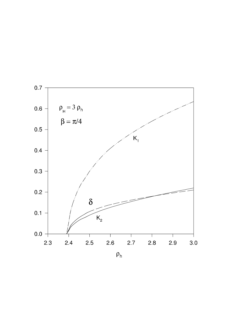
Figure 2: The evolution of the parameters $\delta,K_{1}\equiv K(0),K_{2}\equiv\tilde{K}(0)$ is shown as function of $\rho_{h}$ for $\rho_{H}=3\rho_{h}$.

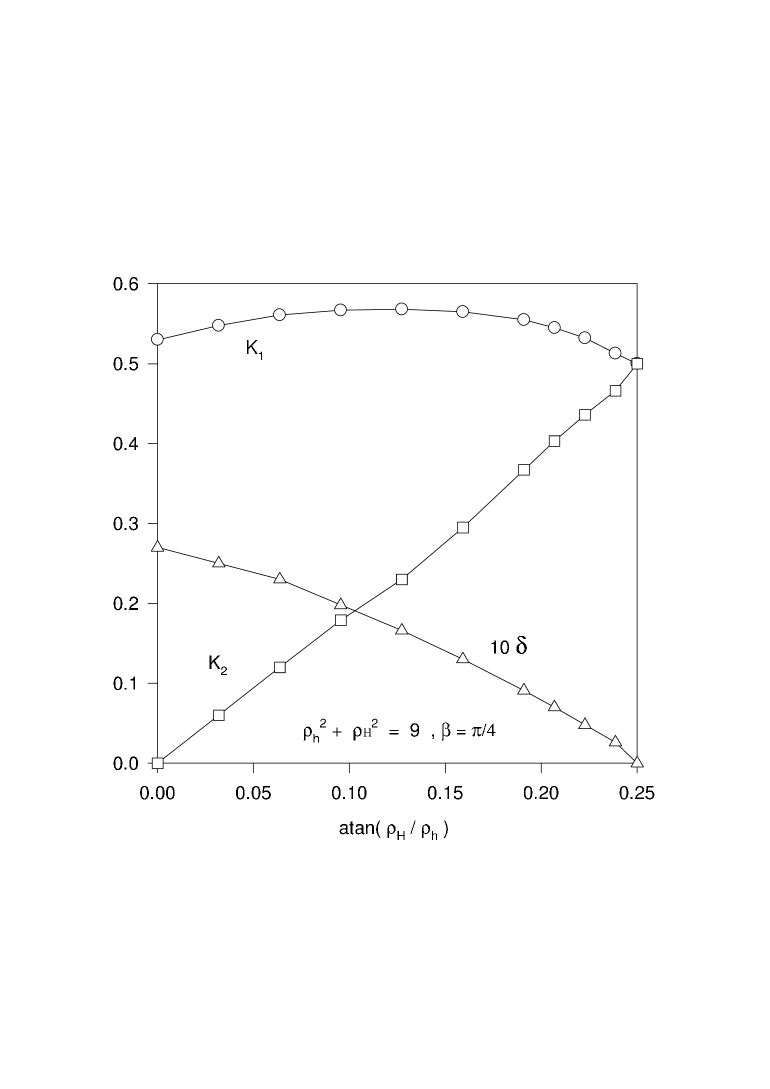
Figure 3: The evolution of the parameters $\delta,K_{1}\equiv K(0),K_{2}\equiv\tilde{K}(0)$ is shown as function of $\rho_{H}/\rho_{h}$ for $\rho_{H}^{2}+\rho_{h}^{2}=9$.

The results of [13] show the existence of a smooth surface in the $\rho_{1},\rho_{2},\beta$-parameter space inside of which only sphaleron solution exist while sphaleron and bisphaleron coexist outside, the bifurcation taking place on the surface. The critical surface can be determined only numerically by studying a few parameters characterizing the bisphaleron solutions, namely the values $\delta,K(0),\tilde{K}(0)$, as functions of $\beta,\epsilon_{1,2,3}$. Varying one of these parameters and fixing the other three, a critical point is determined when $\delta,K(0),\tilde{K}(0)$ approach zero. This is done on Fig. 2 for $\beta=\pi/4$ , $\epsilon_{3}=0$ and $\rho_{H}=3\rho_{h}$. The critical point then corresponds to $\rho_{H}\approx 2.397$. It is worth noticing that bisphaleron solutions with $\delta=0$ but $K(x)\neq 0$, $\tilde{K}(x)\neq 0$ also occur outside the critical surface. This is illustrated on Fig.3 where we set $\rho_{H}^{2}+\rho_{h}^{2}=9$ and vary $\Theta\equiv atan(\rho_{H}/\rho_{h})$. Clearly, $\delta$ goes to zero in the limit $\Theta\rightarrow\pi/4$. The figures 2 and 3 are complementary to the ones presented in [12, 13]

The main feature of the bisphaleron solutions in the 2DSM is that the angle $\tilde{\phi}=\arctan(\tilde{K}/\tilde{H})$ increases monotonically from $0$ (for $x=0$) to $\pi-q$ (for $x=\infty$) while $\phi=\arctan(K/H)$ decreases from $0$ to $\pi(q-1)$; that is to say that these solutions of lowest energy have $k=1$ in (21). In fact, non trivial solutions with $k=0$ were discovered in [12] but since they have a higher energy, they are likeky less interesting as far as the energy barrier is concerned.

4.3 2DSM, case $\epsilon_{3}\neq 0$

The construction of solutions in the domain $\rho_{h},\rho_{H},\beta,\epsilon_{3}$ and the study of the critical hypersurface in this four-parameter space is a vast task. For definiteness, we have limited our investigations to the case $\rho_{h}=3.0$ and to two values of $\beta$, namely $\beta=\pi/4$ and $\beta=3\pi/8$.

We first discuss the results for $\beta=\pi/4$, i.e. $v1=v_{2}$. Here are a few ”points“ on the bifurcation line correponding to $\beta=\pi/4$ :

$$(\rho_{h},\rho_{H}):(10,7.6)\ ,\ (3.0,7.08)\ ,\ (5.0,6.08)\ ,\ (5.585,5.585)$$ (24)

Our main concern is to determine how this domain of the $\rho_{h},\rho_{H}$ plane evolves with $\epsilon_{3}$. The result is illustrated by Fig. 1. where the physical domain is delimited by the solid lines. The sphaleron-bisphaleron bifurcation line is represented by the solid line with bullets and the domains where sphaleron only exist is indicated, as well as the domain where sphaleron and bisphaleron coexist. The critical line separating these two regions clearly exhibits two different behaviours on the domain of parameters considered : for $6.2\leq\rho_{H}\leq 8$, the critical line is roughly a function increasing linearly with the coupling constant $\epsilon_{3}$. As a consequence, the critical line intersect the lower line delimiting the physical domain, for instance at $\rho_{H}\approx 6.22\ ,\ \epsilon_{3}\approx-15.0$. Clearly, for the negative values of $\epsilon_{3}$, the the minimal mass of $M_{H}$ (with all other parameters fixed) for which bisphaleron exist is lowered by the presence of a direct interaction between the BEH-fields. For $8.0<\rho_{H}<10.0$ the critical lines develops a plateau at $\epsilon_{3}\approx 10.0$ and $\rho_{H,cr}$ depends only weakly of $\epsilon_{3}$. For some unknown reason, the numerical analysis become very difficult when the critical line appraoches the limit of the physical domain.

The behavior of the critical line turns out to be completely different for $\beta=2\pi/8$, in this case, the limit of the physical domain is indicated by the dashed lines and the critical line bu the dashed line with the triangles. In contrast to the case $\beta=\pi/4$ we see here that the critical value $\rho_{H,cr}$ decreases roughly linearly with $\epsilon_{3}$. For $\epsilon_{3}>0$ the barrier turns out to be a bisphaleron for lower values of $\rho_{H}$ than in the $\epsilon_{3}=0$ case. Here, the critical line seems to cross the two lines determining the physical domain where it naturally terminate.

We further studied the critical phenomenon for $3\pi/8<\beta<\pi/4$ and observed a smooth evolution of the critical lines displayed in Fig. 1.

5 Conclusion

The lagrangian considered in this note leads to a tricky system of six differential equations with boundary conditions and depending effectively on four parameters. Many types of non-trivial solutions can be constructed numerically [12] but, at the moment, the ones with lowest energy are identified as the sphaleron or the bisphaleron, depending on the different coupling constants. The determination of the critical hypersurface of bifurcation in the space of parameters constitutes a huge task which can be studied only numerically. The problem is for a large part academical; however at the moment, the theoretical limits on the BEH-boson masses obtained in the two-doublets extension of the electroweak model, do not yet exclude that the energy barrier between topologically different vacua could be determined by a bisphaleron. A few years ago, it was already pointed out that the minimal mass of the neutral BEH-fields for the barrier to be of the bisphaleron type is considerably lower in the two-doublets model (without direct interaction of the doublets in the potential) than in the minimal, one-doublet model. The calculations reported here suggest that, if a custodially-invariant coupling term is supplemented to the potential, the critical mass $\rho_{H,cr}$ varies roughly linearly with the new coupling constant $\epsilon_{3}$. The supplementary coupling constant cannot off course be arbitrarily large, but on the physical domain, the critical value $\rho_{H,cr}$ indeed dimnishes, all other masses being fixed. Off course, many other terms can be added in the potential [11] and it could be that bisphaleron solution exist for still lower masses of the neutral BEH-field when terms allowing for charged BEH-fields are considered as well.

Acknowledgements This work started from several discussions with Michel Herquet. I gratefully acknowledge him for these discussions, his interest in the topic and for numerous private communications about his own reseach [16].

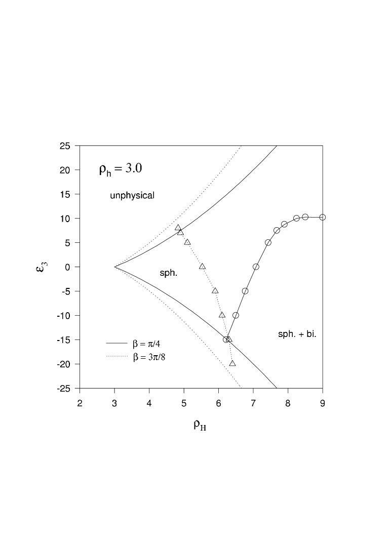
Figure 1: The physical domain corresponding to the case $\rho_{h}=3.0$, $\beta=\pi/4$ (resp. $\beta=3\pi/8$) are represented by the solid (resp. dashed) line in the $\rho_{H},\epsilon_{3}$ plane. The line with bullets (resp. triangle) represents the sphaleron-bisphaleron bifurcation.

References

- [1] ’t Hooft, G., Symmetry breaking through Bell-Jackiw Anomalies, Phys. Rev. Lett.37, 8 (1976).
- [2] Rubakov, V.A., Shaposhnikov, M. E., Electroweak baryon number non-conservation in the early universe and in high energy collisions, Phys. Usp.39, 461 (1996), hep-ph/9603208.
- [3] Trodden, M., Electroweak baryogenesis, CWRU-P6-98 , hep-ph/9803479.
- [4] Kuzmin, V. A., Rubakov, V. A., and Shaposhnikov, M. E., On anomalous electroweak baryon-number non-conservation in the early universe, Phys. Lett. B155, 36 (1985).
- [5] Manton, N. S., Topology in the Weinberg-Salam theory, Phys. Rev. D28, 2019 (1983).
- [6] Klinkhamer, F. R., and Manton, N. S., A saddle-point solution in the Weinberg-Salam theory, Phys. Rev. D30, 2212 (1984).
- [7] Kunz, J., and Brihaye, Y., (1989), New sphalerons in the Weinberg-Salam theory, Phys. Lett. B216, 353 (1989).
- [8] Yaffe, L. G., Static solutions of SU(2)-Higgs theory, Phys. Rev. D40, 3463 (1989).
- [9] Brihaye, Y., and Kunz, J., A sequence of new classical solutions in the Weinberg-Salam model, Mod. Phys. Lett. A4, 2723 (1989).
- [10] Monig, K., Limits on Present and Future, Delphi collaboration report 98-14 PHYS 764, (1998).
- [11] Dawson, S, Gunion, J.F., Haber, H.E. and Kane, G.L., The Higgs Hunters’guide, Frontiers in Physics, Addison-Wesley (1990).
- [12] Bachas, C., Tinyakov, P. and Tomaras, T.N., On spherically-symmetric solutions in the two-Higgs standard model, Phys. Lett. B385, 237 (1996).
- [13] Kleihaus, B., Energy barrier in the two-Higgs model, Mod. Phys. Lett. A 14, 1431 (1999).
- [14] Kastening, B., Peccei, R. and Zang, X., Sphaleron in the two doublet Higgs model, Phys. Lett. B 266, 413 (1991).
- [15] Grant, J. and Hindmarsh M., Sphaleron in Two Higgs Doublets Theories, Phys. Rev. D 64, 016002 (2001).
- [16] Herquet, M., Symétries custodiales dans les modèles à deux doublets de Higgs, DEA Thesis, Université Catholique de Louvain (Sept. 2004).
- [17] Akiba, T., Kikuchi H., and Yanagida, T., The free energy of the sphaleron in the Weinberg-Salam model, Phys. Rev. D40, 179 (1989).
- [18] Brihaye, Y., and Kunz, J., Normal modes around the SU(2) sphalerons, Phys. Lett. B249, 90 (1990).