MHV Rules for Higgs Plus Multi-Parton Amplitudes

Abstract:

We present MHV-rules for constructing perturbative amplitudes for a Higgs boson and an arbitrary number of partons. We give explicit expressions for amplitudes involving a Higgs and three negative helicity partons and any number of positive helicity partons - the NMHV amplitudes. We also present a recursive formulation of MHV rules that incorporates the Higgs, quarks and gluons. The recursion relations are valid for all non-MHV amplitudes. The general results agree numerically with all of the available Higgs $+$ $n$-parton amplitudes and in some cases provide considerably shorter expressions.

1 Introduction

There is a new and poweful framework for computing gauge theory amplitudes – ‘MHV rules’ [1]. These rules provide analternative and more compact diagrammatic expansion compared to the conventional Feynman rules. The basic building blocks are the colour-ordered $n$-point vertices which are connected by scalar propagators. These vertices are off-shell continuations of the maximally helicity-violating (MHV) $n$-gluon scattering amplitudes of Parke and Taylor [2]. They contain precisely two negative helicity gluons. By connecting MHV vertices, amplitudes involving more negative helicity gluons can be built up. The MHV rules are inspired by the interpretation of supersymmetric Yang-Mills (SYM) theory and QCD as a topological string propagating in twistor space [3].

The original MHV rules for gluons [1] have been extended to amplitudes with fermions [4]. In fact, they straighforwardly apply to all particles in the full ${\cal N}=4$ supermultiplet by reading the appropriate terms from the general expression for the MHV ${\cal N}=4$ supervertex of Nair [5] using the algorithm described in [6, 7].

MHV rules have been shown to work at the loop-level for supersymmetric theories and, building on the earlier work of Bern et al [8, 9], there has been enormous progress in computing multi-leg loop amplitudes in ${\cal N}=4$ [11, 10, 12, 13, 14, 15, 19, 16, 17, 18] and ${\cal N}=1$ [20, 22, 21, 23] SYM theories.

At the same time, the MHV rules have given new tree-level gauge-theory results for non-MHV amplitudes involving gluons [27, 25, 26], and fermions [4, 6, 28, 29]. It is of great phenomenological interest to extend the method to processes involving massive particle like the Higgs [30], electroweak vector bosons [31] and heavy quarks. Processes like these, together with those involving massive supersymmetric particles, are of vital importance for experiments at the LHC and elsewhere.

It has been shown in [30] that Higgs plus gluons amplitudes can be computed efficiently by introducing an effective operator and using a modified set of MHV rules. Approximating Higgs interactions by coupling via a top loop is strongly supported by current precision electroweak data which predicts the the Higgs is considerably lighter than $2m_{t}\approx 360$ GeV; currently $m_{H}<260$ GeV at 95% confidence level [32]. In this case it is an excellent approximation to integrate out the heavy top quark, summarising its effects via the dimension-five operator $H\mathop{\rm tr}\nolimits G_{\mu\nu}G^{\mu\nu}$ [33, 34]. This operator can then be ‘dressed’ by standard QCD vertices in order to generate Higgs plus multi-parton amplitudes.

The purpose of this paper is to complete the work begun in [30] by computing Higgs to multi-parton amplitudes with one and two quark-antiquark pairs. In section 2 we review the construction of the amplitudes for Higgs and gluons. The MHV rules arise from splitting the effective Higgs-gluons interaction into two pieces, one holomorphic, and one anti-holomorphic. These two pieces can be calculated separately using scalar MHV graphs and then must be added together to form the full Higgs amplitude. Here we generalise this method to allow fermions in the Higgs plus multi-parton amplitudes and show how MHV and $\overline{\text{MHV}}$ vertices for one and two quark-antiquark pairs can be derived from supersymmetry and extend the MHV rules for Higgs and gluons to the case including fermions.

In Section 3 we write down the MHV amplitudes for a self-dual scalar $\phi$ into a quark-antiquark pair and gluons and then use these to compute the corresponding NMHV amplitudes. We then show that these results agree with the known analytic expressions for $n\leq 5$ partons at tree-level. In Section 4 we consider interactions containing two quark-anti-quark pairs. We use the new MHV vertices to compute the eight NMHV helicity amplitudes which are then shown to reproduce the known analytic formula for $n\leq 5$ partons.

Finally Section 5 generalises the recursive formulation of non-MHV gluonic amplitudes of Bena, Bern and Kosower [26] to the case of amplitudes with fermions and/or scalars. We then use these formulae to find numerical values for NNMHV amplitudes with Higgs and a single quark-antiquark pair. This completes the checks necessary for all amplitudes with up to $n\leq 5$ partons. The recursion relations are, of course, valid for $n>5$ partons. Our findings are then summarised in the conclusions.

For the sake of clarity and completeness, we include three appendices. Appendix A defines our conventions regarding helicity spinor formalism. Appendix B defines colour ordered amplitudes which we study in this paper. Finally Appendix C provides a recursive proof of the vanishing of all $A_{n}(\phi,q^{\lambda},g^{+}_{2},\ldots,g^{+}_{n-1},\bar{q}^{-\lambda}_{n})$ amplitudes using the Berends-Giele currents [35].

2 MHV amplitude towers including fermions

The MHV rules arise from splitting the effective Higgs-gluons interaction into two pieces, one holomorphic, and one anti-holomorphic. The amplitudes generated by these two terms should be calculated separately using scalar MHV graphs and then must be added together to form the full Higgs amplitude. In this way the picture [30] of the “two towers” of MHV and $\overline{\text{MHV}}$ amplitudes to form the full Higgs amplitude emerges.

2.1 The model

In the Standard Model the Higgs boson couples to gluons through a fermion loop. The dominant contribution is from the top quark. For large $m_{t}$, the top quark can be integrated out leading to the effective interaction [34, 33],

$${\cal L}_{\scriptscriptstyle H}^{\rm int}={C\over 2}\,H\mathop{\rm tr}\nolimits G_{\mu\nu}\,G^{\mu\nu}\ .$$ (1)

In the Standard Model, and to leading order in $\alpha_{s}$, the strength of the interaction is given by $C=\alpha_{s}/(6\pi v)$, with $v=246$ GeV.

It was explained in [30] that the MHV or twistor-space structure of the Higgs-plus-gluons amplitudes is best elucidated by dividing the Higgs coupling to gluons, eq. (1), into two terms, containing purely selfdual (SD) and purely anti-selfdual (ASD) gluon field strengths,

$$G_{\scriptscriptstyle SD}^{\mu\nu}={\textstyle{1\over 2}}(G^{\mu\nu}+{}^{*}G^{\mu\nu})\ ,\quad G_{\scriptscriptstyle ASD}^{\mu\nu}={\textstyle{1\over 2}}(G^{\mu\nu}-{}^{*}G^{\mu\nu})\ ,\quad{}^{*}G^{\mu\nu}\equiv{\textstyle{i\over 2}}\epsilon^{\mu\nu\rho\sigma}G_{\rho\sigma}\ .$$ (2)

This division can be accomplished by considering $H$ to be the real part of a complex field $\phi={1\over 2}(H+iA)$, so that

$${\cal L}^{\rm int}_{H,A} = {C\over 2}\Bigl{[}H\mathop{\rm tr}\nolimits G_{\mu\nu}\,G^{\mu\nu}+iA\mathop{\rm tr}\nolimits G_{\mu\nu}\,{}^{*}G^{\mu\nu}\Bigr{]}$$ (3)

$$= C\Bigl{[}\phi\mathop{\rm tr}\nolimits G_{{\scriptscriptstyle SD}\,\mu\nu}\,G_{\scriptscriptstyle SD}^{\mu\nu}+\phi^{\dagger}\mathop{\rm tr}\nolimits G_{{\scriptscriptstyle ASD}\,\mu\nu}\,G_{\scriptscriptstyle ASD}^{\mu\nu}\Bigr{]}\ .$$ (4)

The important observation of [30] was that, due to selfduality, the amplitudes for $\phi$ plus $n$ gluons, and those for $\phi^{\dagger}$ plus $n$ gluons, separately have a simpler structure than the amplitudes for $H$ plus $n$ gluons. MHV rules are constructed for $\phi$ plus $n$ gluons amplitudes and for for $\phi^{\dagger}$ plus $n$ gluons separately. Then since $H=\phi+\phi^{\dagger}$, the Higgs amplitudes can be recovered as the sum of the $\phi$ and $\phi^{\dagger}$ amplitudes.

Quarks do not enter the $HGG$ effective vertex (1) or (4) directly, they couple to it only through gluons. The division of eq. (1) into selfdual and anti-selfdual terms, dictated by eq. (4) will continue to be the guiding principle for constructing MHV rules for the Higgs plus quarks and gluons amplitudes. In fact, in this section we will derive the MHV rules for the Higgs with gluons and quarks from the simpler MHV rules of [30] for amplitudes with the Higgs and gluons only.

Throughout the paper we use a standard colour decomposition for all amplitudes ${\cal A}_{n}$ in terms of colour factors ${\cal T}_{n}$ and purely kinematic partial amplitudes $A_{n}$ as reviewed in Appendix B. Only these colour-ordered kinematic amplitudes $A_{n}$ need to be calculated. The full amplitudes can be assembled from color-ordered amplitudes $A_{n}$ and known expressions for the colour factors ${\cal T}_{n}$ as described in Appendix B.

Hence without loss of generality from now on we will concentrate on the colour-ordered partial amplitudes $A_{n}$ involving partons (gluons, quark-antiquark pairs, gluinos) plus the single colourless scalar field which can be $H$, $\phi$ or $\phi^{\dagger}$.

The kinematic amplitudes $A_{n}$ have the colour information stripped off and hence do not distinguish between fundamental quarks and adjoint gluinos. Hence, if we know kinematic amplitudes involving gluinos in a supersymmetric theory, we automatically know kinematic amplitudes with quarks,

$$A_{n}(H,q^{+},\ldots,\bar{q}^{\,-},\ldots,g^{+},\ldots,g^{-})\,=\,A_{n}(H,\Lambda^{+},\ldots,\Lambda^{-},\ldots,g^{+},\ldots,g^{-})$$ (5)

Here $q^{\pm}$, $\bar{q}^{\pm}$, $g^{\pm}$, $\Lambda^{\pm}$ denote quarks, antiquarks, gluons and gluinos of $\pm$ helicity, and $H$ represents the colourless scalar $H$, $\phi$, $\phi^{\dagger}$ or simply nothing. By this we mean that (5) is valid with or without the scalar field, this is because the colourless scalar does not modify the colour decomposition. We conclude from (5) that knowing kinematic amplitudes in a supersymmetric theory with gluinos allows us to deduce immediately non-supersymmetric amplitudes with quarks and antiquarks.

MHV rules were formulated in [30] for amplitudes with the Higgs and $n$ gluons. In the following section we will show that these rules uniquely determine the MHV rules for the Higgs plus all partons (i.e. gluons and quarks). More precisely, the MHV amplitudes with the Higgs and gluons determine the MHV amplitudes with the Higgs, gluinos and gluons via supersymmetric Ward identities. Then (5) turns gluinos into quarks in a non-supersymmetric theory.

2.2 MHV amplitudes

We start with the (anti)-MHV amplitudes for the Higgs and gluons from [30]. First, the decomposition of the $HGG$ vertex into the selfdual and the anti-selfdual terms eq. (4), guarantees that the whole class of helicity amplitudes must vanish [30]:

$$A_{n}(\phi,g_{1}^{\pm},g_{2}^{+},g_{3}^{+},\ldots,g_{n}^{+})=0\,,\quad A_{n}(\phi^{\dagger},g_{1}^{\pm},g_{2}^{-},g_{3}^{-},\ldots,g_{n}^{-})=0\,,$$ (6)

for all $n$.

The amplitudes, with precisely two negative helicities, $\phi\,g^{-}g^{+}\ldots g^{+}g^{-}g^{+}\ldots g^{+}$, are the first non-vanishing $\phi$ amplitudes. These amplitudes will be referred to as the $\phi$-MHV amplitudes. General factorization properties now imply that they have to be extremely simple [30], they read

$$A_{n}(\phi,g_{1}^{+},g_{2}^{+},\ldots,g_{p}^{-},\ldots,g_{q}^{-},\ldots,g_{n}^{+})={{\left\langle p\,q\right\rangle}^{4}\over\left\langle 1\,2\right\rangle\left\langle 2\,3\right\rangle\cdots\left\langle n-1,\,n\right\rangle\left\langle n\,1\right\rangle}\,,$$ (7)

Here only legs $p$ and $q$ have negative helicity. This expression is valid for all $n$. Besides the correct collinear and multi-particle factorization behavior, these amplitudes also correctly reduce to pure QCD MHV amplitudes as the $\phi$ momentum approaches zero. In fact, the expressions (7) for $\phi$-MHV $n$-gluon amplitudes are exactly the same as the MHV $n$-gluon amplitudes in pure QCD. The only difference of (7) with pure QCD is that the total momentum carried by gluons, $p_{1}+p_{2}+\ldots+p_{n}=-p_{\phi}$ is the momentum carried by the $\phi$-field and is non-zero. This momentum makes the Higgs case well-defined on-shell for fewer legs than in the pure QCD case. The first few $\phi$ amplitudes have the form,

$$A_{2}(\phi,g_{1}^{-},g_{2}^{-}) = {{\left\langle 1\,2\right\rangle}^{4}\over\left\langle 1\,2\right\rangle\left\langle 2\,1\right\rangle}=-{\left\langle 1\,2\right\rangle}^{2},$$ (8)

$$A_{3}(\phi,g_{1}^{-},g_{2}^{-},g_{3}^{+}) = {{\left\langle 1\,2\right\rangle}^{4}\over\left\langle 1\,2\right\rangle\left\langle 2\,3\right\rangle\left\langle 3\,1\right\rangle}={{\left\langle 1\,2\right\rangle}^{3}\over\left\langle 2\,3\right\rangle\left\langle 3\,1\right\rangle}\,,$$ (9)

$$A_{4}(\phi,g_{1}^{-},g_{2}^{-},g_{3}^{+},g_{4}^{+}) = {{\left\langle 1\,2\right\rangle}^{4}\over\left\langle 1\,2\right\rangle\left\langle 2\,3\right\rangle\left\langle 3\,4\right\rangle\left\langle 4\,1\right\rangle}\,.$$ (10)

Since the MHV amplitudes (7) have an identical form to the corresponding amplitudes of pure Yang-Mills theory, [30] argued that their off-shell continuation should also identical to that proposed in the pure-glue context in [1]. Everywhere the off-shell leg $i$ carrying momentum $P_{i}$ appears in (7), we let the corresponding holomorphic spinor be $\lambda_{i,\alpha}=(P_{i})_{\alpha\dot{\alpha}}\xi^{\dot{\alpha}}$. Here $\xi^{\dot{\alpha}}$ is an arbitrary reference spinor, chosen to be the same for all MHV diagrams contributing to the amplitude.

We are now ready to discuss MHV amplitudes with gluons and fermions. To this end we first consider a pure ${\cal N}=1$ supersymmetric Yang-Mills (without the Higgs or quarks). An MHV amplitude $A_{n}=A_{l+2m}$ with $l$ gluons, $g$, and $2m$ gluinos, $\Lambda$, in the ${\cal N}=1$ pure gauge theory exists only for $m=0,1,2$. This is because it must have precisely $n-2$ particles with positive helicity and $2$ with negative helicity, and gluinos always come in pairs with helicities $\pm{1\over 2}$. Hence, there are three types of MHV tree amplitudes in the ${\cal N}=1$ pure gauge theory:

$$A_{n}(g_{p}^{-},g_{q}^{-})\ ,\quad A_{n}(g_{t}^{-},\Lambda_{r}^{-},\Lambda_{s}^{+})\ ,\quad A_{n}(\Lambda_{t}^{-},\Lambda_{s}^{+},\Lambda_{r}^{-},\Lambda_{q}^{+})\ .$$ (11)

The MHV purely gluonic amplitude is [2, 35]:

$$A_{n}(g_{p}^{-},g_{q}^{-})=\ {\langle{p~{}q}\rangle^{4}\over\prod_{i=1}^{n}\langle{i~{}i+1}\rangle}\ ,$$ (12)

where $\lambda_{n+1}\equiv\lambda_{1}$. For notational simplicity in this and the following expressions for MHV amplitudes we do not show explicitly the positive helicity gluons $g^{+}$. The MHV amplitude with two external fermions and $n-2$ gluons is

$$A_{n}(g_{t}^{-},\Lambda_{r}^{-},\Lambda_{s}^{+})=\ {\langle{t~{}r}\rangle^{3}\ \langle{t~{}s}\rangle\over\prod_{i=1}^{n}\langle{i~{}i+1}\rangle}\ ,\quad A_{n}(g_{t}^{-},\Lambda_{s}^{+},\Lambda_{r}^{-})=\ -\ {\langle{t~{}r}\rangle^{3}\ \langle{t~{}s}\rangle\over\prod_{i=1}^{n}\langle{i~{}i+1}\rangle}\ ,$$ (13)

where the first expression corresponds to $r<s$ and the second to $s<r$ (and $t$ is arbitrary). The MHV amplitudes with four fermions and $n-4$ gluons on external lines are

$$A_{n}(\Lambda_{t}^{-},\Lambda_{s}^{+},\Lambda_{r}^{-},\Lambda_{q}^{+})=\ {\langle{t~{}r}\rangle^{3}\ \langle{s~{}q}\rangle\over\prod_{i=1}^{n}\langle{i~{}i+1}\rangle}\ ,\quad A_{n}(\Lambda_{t}^{-},\Lambda_{r}^{-},\Lambda_{s}^{+},\Lambda_{q}^{+})=\ -\ {\langle{t~{}r}\rangle^{3}\ \langle{s~{}q}\rangle\over\prod_{i=1}^{n}\langle{i~{}i+1}\rangle}\$$ (14)

The first expression in (14) corresponds to $t<s<r<q,$ the second – to $t<r<s<q,$ and there are other similar expressions, obtained by further permutations of fermions, with the overall sign determined by the ordering.

We now recall that expressions (13), (14) are not independent inputs into the MHV programme, they follow from the amplitudes (12) via supersymmetric Ward identities [38, 39, 40, 36, 37].

Supersymmetric Ward identities [38, 39, 40] follow from the fact that, supercharges $Q$ annihilate the vacuum, and hence we have an equation,

$$\langle[Q\,,\,\Lambda^{+}_{k}\ldots g_{r_{1}}^{-}\ldots g_{r_{2}}^{-}\ldots]\rangle\ =\ 0\ ,$$ (15)

where dots indicate positive helicity gluons. In order to make anticommuting spinor $Q$ to be a singlet entering a commutative (rather than anticommutative) algebra with all the fields we contract it with a commuting spinor $\eta$ and multiply it by a Grassmann number $\theta$. This defines a commuting singlet operator $Q(\eta).$ Following [37] we can write down the following susy algebra relations,

$$\begin{split}[Q(\eta)\,,\,\Lambda^{+}(k)]\ =\ -\theta\langle{\eta~{}k}\rangle\,g^{+}(k)\ ,\quad[Q(\eta)\,,\,\Lambda^{-}(k)]\ =\ +\theta[\eta~{}k]\,g^{-}(k)\ ,\\ [Q(\eta)\,,\,g^{-}(k)]\ =\ +\theta\langle{\eta~{}k}\rangle\,\Lambda^{-}(k)\ ,\quad[Q(\eta)\,,\,g^{+}(k)]\ =\ -\theta[\eta~{}k]\,\Lambda^{+}(k)\ .\end{split}$$ (16)

In what follows, the anticommuting parameter $\theta$ will cancel from the relevant expressions for the amplitudes. The arbitrary spinors $\eta_{a},$ $\eta_{\dot{a}},$ will be fixed below. It then follows from (16) that

$$\theta{\langle{\eta~{}k}\rangle}\,A_{n}(g_{r_{1}}^{-},g_{r_{2}}^{-})=\ -\theta{\langle{\eta~{}r_{1}}\rangle}\,A_{n}(\Lambda_{k}^{+},\Lambda_{r_{1}}^{-},g_{r_{2}}^{-})-\,\theta{\langle{\eta~{}r_{2}}\rangle}\,A_{n}(\Lambda_{k}^{+},g_{r_{1}}^{-},\Lambda_{r_{2}}^{-})\ .$$ (17)

The minus signs on the right hand side arise from anticommuting $\theta$ with gluino fields. After cancelling $\theta$ and choosing $\eta$ to be one of the two $r_{j}$ we find from (17) that the purely gluonic amplitude is proportional to the amplitude with two gluinos,

$$A_{n}(g_{r_{1}}^{-},g_{r_{2}}^{-})\ =\ -\,{{\langle{r_{2}~{}r_{1}}\rangle}\over{\langle{r_{2}~{}k}\rangle}}\,A_{n}(\Lambda_{k}^{+},\Lambda_{r_{1}}^{-},g_{r_{2}}^{-})\ =\ -\,{{\langle{r_{1}~{}r_{2}}\rangle}\over{\langle{r_{1}~{}k}\rangle}}\,A_{n}(\Lambda_{k}^{+},g_{r_{1}}^{-},\Lambda_{r_{2}}^{-})\ .$$ (18)

This gives the MHV amplitudes (13). Equations (14) follow from a similar construction.

We can now add the Higgs scalars $\phi$ and $\phi^{\dagger}$ to the construction of MHV amplitudes above. To achieve this, we embed the bosonic effective interaction (4) into a pseudo-supersymmetric theory,

$${\cal L}^{\rm int}=-C\int d^{2}\theta\ \phi\,\mathop{\rm tr}\nolimits W^{\alpha}W_{\alpha}\,-C\,\int d^{2}\bar{\theta}\ \phi^{\dagger}\,\mathop{\rm tr}\nolimits\overline{W}_{\dot{\alpha}}\overline{W}^{\dot{\alpha}}\,.$$ (19)

Here $G_{\scriptscriptstyle SD}^{\mu\nu}$ is the bosonic component of the ${\cal N}=1$ chiral superfield $W_{\alpha}(x,\theta)$, but $\phi$ is not a superfield, it is still a (single component) scalar field $\phi(x)$ which has no superpartners. So, the theory described by (19) is not a supersymmetric theory. However, there is a continuous symmetry group which leaves this action invariant. It is generated by the ‘supercharges’ $Q$ which act non-trivially on gluons and gluinos – precisely as in (16) – and at the same time annihilate the scalar field,

$$[Q(\eta)\,,\,\phi(p)]\ =\ 0\ ,\qquad[Q(\eta)\,,\,\phi^{\dagger}(p)]\ =\ 0\ .$$ (20)

Applying the commutation relations, (19), (20) to equation

$$\langle[Q\,,\,\phi\,\Lambda^{+}_{k}\ldots g_{r_{1}}^{-}\ldots g_{r_{2}}^{-}\ldots]\rangle\ =\ 0\ ,$$ (21)

we find the same relation as in eq. (18), but now for the MHV amplitudes with the Higgs field $\phi$.

We conclude that the from the fact that the purely gluonic MHV amplitudes, (7) and (12) take the same form, the pseudo-supersymmetry Ward identities guarantee that the tree-level $\phi$-MHV amplitudes with fermions and gluons have exactly the same algebraic form as the corresponding MHV amplitudes in pure ${\cal N}=1$ gauge theory, (13) and (14). Hence we now can insert the $\phi$ field on the left hand sides of (13) and (14), and, furthermore, replace gluinos with quarks as in (5).

We need to be slightly more careful in order to deduce the $\phi$-MHV amplitudes with two quark-antiquark pairs of different flavours, i.e. ${A}_{n}(\phi,q^{+},\bar{q}^{\,-},Q^{+},\bar{Q}^{-})$ where $q$ and $Q$ denote the two different quarks. Such amplitudes are obtained from the ${\cal N}=2$ supersymmetric amplitudes ${A}_{n}(\phi,\Lambda_{(1)}^{+},\Lambda_{(1)}^{-},\Lambda_{(2)}^{+},\Lambda_{(2)}^{-})$ where $\Lambda_{(1)}$ and $\Lambda_{(2)}$ are gluinos from two different ${\cal N}=1$ supermultiplets. All such amplitudes can be read off from the general expression for the MHV ${\cal N}=4$ supervertex of Nair [5] using the algorithm described in [6, 7]. The supervertex and the corresponding component vertices comply with the supersymmetric Ward identities in pure ${\cal N}=4$ theory. The Higgs field $\phi$ can always be added to these amplitudes in precisely the same way as above, without changing the expression for the vertex. This follows from promoting the ${\cal N}=4$ or ${\cal N}=2$ supersymmetry to a ‘pseudo’ supersymmetry by augmenting the algebra with the condition (20).

2.3 MHV rules

We have argued that the complete set of MHV amplitudes in QCD coupled to the Higgs field consists of $n$-parton amplitudes made out of one or less scalar field $\phi$, an arbitrary number of gluons and $m=0,1,2$ quark-antiquark pairs. All these amplitudes have precisely two negative helicities. Schematically, they are

$$A_{n}(\phi,g_{p}^{-},g_{q}^{-})\ ,\quad A_{n}(\phi,q_{1}^{-\lambda},g_{r}^{-},\bar{q}_{n}^{\,\lambda})\ ,\quad A_{n}(\phi,q_{1}^{-\lambda_{1}},\bar{Q}_{s}^{\,\lambda_{2}},Q_{s+1}^{-\lambda_{2}},\bar{q}_{n}^{\,\lambda_{1}})\ ,$$ (22)

$$A_{n}(g_{p}^{-},g_{q}^{-})\ ,\quad A_{n}(q_{1}^{-\lambda},g_{r}^{-},\bar{q}_{n}^{\,\lambda})\ ,\quad A_{n}(q_{1}^{-\lambda_{1}},\bar{Q}_{s}^{\,\lambda_{2}},Q_{s+1}^{-\lambda_{2}},\bar{q}_{n}^{\,\lambda_{1}})\ .$$ (23)

Here we have not shown the positive helicity gluons and did not exhibit all different orderings for amplitudes with two quark-antiquark pairs. As before, $Q^{-\lambda_{2}}$ and $\bar{Q}^{\,\lambda_{2}}$ denote the second flavour of (anti)quarks with helicities $\pm\lambda_{2}$.

The first line, eq. (22), gives the $\phi$-MHV amplitudes, and the second line, eq. (23) corresponds to standard QCD MHV amplitudes. The $\overline{\text{MHV}}$ amplitudes are obtained from (eq. (22)) and (eq. (23)) by parity. They are

$$A_{n}(\phi^{\dagger},g_{p}^{+},g_{q}^{+})\ ,\quad A_{n}(\phi^{\dagger},q_{1}^{\lambda},g_{r}^{+},\bar{q}_{n}^{\,-\lambda})\ ,\quad A_{n}(\phi^{\dagger},q_{1}^{\lambda_{1}},\bar{Q}_{s}^{\,-\lambda_{2}},Q_{s+1}^{\lambda_{2}},\bar{q}_{n}^{\,-\lambda_{1}})\ ,$$ (24)

$$A_{n}(g_{p}^{+},g_{q}^{+})\ ,\quad A_{n}(q_{1}^{\lambda},g_{r}^{+},\bar{q}_{n}^{\,-\lambda})\ ,\quad A_{n}(q_{1}^{\lambda_{1}},\bar{Q}_{s}^{\,-\lambda_{2}},Q_{s+1}^{\lambda_{2}},\bar{q}_{n}^{\,-\lambda_{1}})\ ,$$ (25)

where we have not shown the negative helicity gluons.

We start with the amplitudes with no fermions, considered in [30]. The left (red) tower in figure 1 lays out the MHV structure of the $\phi$ plus multi-gluon amplitudes. All non-vanishing amplitudes are labelled with circles. The fundamental $\phi$-MHV vertices, which coincide with the $\phi g^{-}g^{-}g^{+}\ldots g^{+}$ amplitudes, are the basic building blocks and are labelled by red dots. The result of combining $\phi$-MHV vertices with pure-gauge-theory MHV vertices is to produce amplitudes with more than two negative helicities. These amplitudes are represented as red open circles. Each MHV diagram contains exactly one $\phi$-MHV vertex; the rest are pure-gauge-theory MHV vertices. The vertices are combined with scalar propagators. The MHV-drift is always to the left and upwards. Collectively, these amplitudes form the holomorphic (or MHV) tower of accessible amplitudes.

The corresponding amplitudes for $\phi^{\dagger}$ are shown in the right (green) tower in figure 1. They can be obtained by applying parity to the $\phi$ amplitudes. For practical purposes this means that we compute with $\phi$, and reverse the helicities of every gluon. Then we let $\left\langle i\,j\right\rangle\leftrightarrow\left[j\,i\right]$ to get the desired $\phi^{\dagger}$ amplitude. The set of building-block amplitudes are therefore anti-MHV. Furthermore, the amplitudes with additional positive-helicity gluons are obtained by combining with anti-MHV gauge theory vertices. The anti-MHV-drift is always to the right and upwards. Collectively, these amplitudes form the anti-holomorphic (or anti-MHV) tower of accessible amplitudes.

The allowed helicity states are shown in figure 1 and are composed of both holomorphic and anti-holomorphic structures. Where the two towers do not overlap, the amplitudes for the real Higgs boson with gluons coincide with the $\phi$ ($\phi^{\dagger}$) amplitudes. On the other hand, where the towers overlap, we add the $\phi$ and $\phi^{\dagger}$ amplitudes.

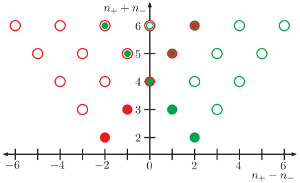
Figure 1: The structure of Higgs plus multi-gluon amplitudes obtained by combining the MHV tower for $\phi+n$ gluons and the anti-MHV tower of $\phi^{\dagger}+n$ gluon amplitudes.

Next we consider amplitudes with one quark-antiquark pair. Helicity must be conserved along the quark line so the all plus configuration is trivially zero. The case where antiquark has opposite helicity to the quark and all gluons have positive helicity is also zero, see Appendix C for a proof which does not appeal to supersymmetry. So the first non-vanishing amplitude is again with two negative helicities and one of them lying on a gluon: $A_{n}(\phi,q^{\lambda}_{1},\ldots,g^{-}_{s},\ldots,\bar{q}^{\,-\lambda}_{n})$. This is precisely the second $\phi$-MHV amplitude in eq. (24).

The structure of the two MHV towers for amplitudes with the Higgs and one quark-antiquark pair is set out in figure 2. Here the $\phi$-MHV amplitudes are represented by filled red dots and the $\phi$-$\overline{\text{MHV}}$ by filled green dots. The open red(green) dots are amplitudes which can be found by combining two or more MHV($\overline{\text{MHV}}$) vertices. The $\overline{\text{MHV}}$ amplitudes can be obtained directly from the MHV amplitudes via parity transformation. Once again, Higgs amplitudes are given directly by $\phi$ or $\phi^{\dagger}$ amplitudes, or by adding them when the towers overlap.

The case of two quark-antiquark pairs proceeds in an almost identical way. Helicity conservation along both quark lines immediately leads us to the fact that the first non-zero $\phi$-amplitude contains two negative helicities, $A(q^{\lambda_{1}},\bar{q}^{-\lambda_{1}},Q^{\lambda_{2}},\bar{Q}^{-\lambda_{2}})$, and this is precisely the third $\phi$-MHV amplitude in eq. (24). Figure 3 shows the structure of the MHV and $\overline{\text{MHV}}$ towers. In the same way as before we add together the MHV(red) and $\overline{\text{MHV}}$(green) amplitudes to get the Higgs amplitudes.

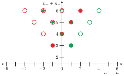
Figure 2: The structure of Higgs plus multi-gluon plus quark-antiquark pair amplitudes obtained by combining the MHV tower for $\phi+q\bar{q}+n$ gluons and the anti-MHV tower of $\phi^{\dagger}+q\bar{q}+n$ gluon amplitudes.

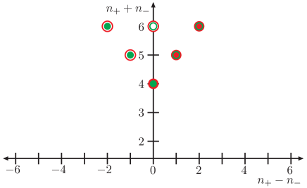
Figure 3: The structure of Higgs plus multi-gluon plus two quark-antiquark pair amplitudes obtained by combining the MHV tower for $\phi+q\bar{q}+Q\bar{Q}+n$ gluons and the anti-MHV tower of $\phi^{\dagger}+q\bar{q}+Q\bar{Q}+n$ gluon amplitudes.

In all three figures we combine the MHV amplitudes at tree level by first continuing appropriate lines off-shell in the same way as in [1], and then connecting them by scalar propagators. The propagators connecting gluon or fermion lines are always of the scalar type, $1/q^{2}$, as explained in [4, 6].

3 Amplitudes with one quark-antiquark pair

When there is a single quark-antiquark pair, the tree-level amplitude can be decomposed into colour-ordered amplitudes as follows,

$${\cal A}_{n}(\phi,\{p_{i},\lambda_{i},a_{i}\},\{p_{j},\lambda_{j},i_{j}\})$$

$$=iCg^{n-2}\sum_{\sigma\in S_{n-2}}(T^{a_{\sigma(2)}}\cdots T^{a_{\sigma(n-1)}})_{i_{1}i_{n}}\,A_{n}(\phi,1^{\lambda},\sigma(2^{\lambda_{2}},\ldots,{(n-1)}^{\lambda_{n-1}}),n^{-\lambda})\,.$$

where $S_{n-2}$ is the set of permutations of $(n-2)$ gluons. Gluons are characterised with adjoint colour label $a_{i}$, momentum $p_{i}$ and helicity $\lambda_{i}$ for $i=1,\ldots,n-1$, while the fermions carry fundamental colour label $i_{j}$, momentum $p_{j}$ and helicity $\lambda_{j}$ for $j=1,n$. By current conservation, the quark and antiquark helicities are related such that $\lambda_{1}=-\lambda_{n}\equiv\lambda$ where $\lambda=\pm{1\over 2}$.

3.1 MHV Amplitudes

\psfrag{1}{$1^{\lambda}$}\psfrag{r-}{$r^{-}$}\psfrag{n}{$n^{-\lambda}$}\psfrag{phi}{$\phi$}\includegraphics[width=142.26378pt]{2Qmhv.eps}

Figure 4: MHV vertices for $\phi$ and one quark pair. The quark line is represented by the red dot-dashed line where $\pm\lambda_{1}$ are the helicities of the quark and anti-quark. The negative helicity gluon is represented as a solid black line.

There are two MHV vertices for a scalar, $\phi$, and a quark pair indicated in figure 4. Together with the usual MHV vertices (23) and a scalar with gluons (7) we can begin to construct tree-level Higgs amplitudes with one quark pair. The expressions for the new vertices are:

$$A_{n}(\phi,q^{-}_{1},\ldots,g^{-}_{r},\ldots,\bar{q}^{+}_{n}) = \frac{\left\langle r\,1\right\rangle^{3}\left\langle r\,n\right\rangle}{\prod_{l=1}^{n}\left\langle l\,l+1\right\rangle},$$ (27)

$$A_{n}(\phi,q^{+}_{1},\ldots,g^{-}_{r},\ldots,\bar{q}^{-}_{n}) = \frac{\left\langle r\,1\right\rangle\left\langle r\,n\right\rangle^{3}}{\prod_{l=1}^{n}\left\langle l\,l+1\right\rangle}.$$ (28)

The $\overline{\text{MHV}}$ amplitudes can be obtained by the following parity transformation:

$$A_{n}(\phi^{\dagger},q^{\lambda}_{1},\ldots,g^{+}_{r},\ldots,\bar{q}^{-\lambda}_{n})=(-1)^{n}\left(A_{n}(\phi,q^{-\lambda}_{1},\ldots,g^{-}_{r},\ldots,\bar{q}^{\lambda}_{n})\right)^{*}$$ (29)

Besides having the correct collinear and multi-particle factorization behavior, these amplitudes also correctly reduce to pure QCD amplitudes as the $\phi$ momentum approaches zero. As discussed in Sec. 2, eqs. (27) and  (28) follow from the analagous MHV amplitudes for $\phi-$gluon interactions (7) by supersymmetry. Alternatively, eqs. (27) and (28) can be proved recursively, along the lines of the proof in the QCD case [35], or using the light-cone recursive currents of ref. [41].

3.1.1 $H\to q^{-}g^{-}g^{+}\bar{q}^{+}$

This amplitude corresponds to $n_{+}+n_{-}=4$, $n_{+}-n_{-}=0$. As we see from figure 2, the amplitude receives contributions from both the MHV and $\overline{\text{MHV}}$ towers, so that

$$A_{n}(H,q^{-}_{1},g^{-}_{2},g^{+}_{3},\bar{q}^{+}_{4}) = A_{n}(\phi,q^{-}_{1},g^{-}_{2},g^{+}_{3},\bar{q}^{+}_{4})+A_{n}(\phi^{\dagger},q^{-}_{1},g^{-}_{2},g^{+}_{3},\bar{q}^{+}_{4})$$ (30)

$$= -\frac{[34]^{2}[13]}{[12][23][41]}-\frac{\left\langle 1\,2\right\rangle^{2}\left\langle 2\,4\right\rangle}{\left\langle 2\,3\right\rangle\left\langle 3\,4\right\rangle\left\langle 4\,1\right\rangle}.$$

This expression agrees with the known analytic formulae of Ref. [42].

3.2 NMHV Amplitudes

We continue by deriving the Next-to-MHV (NMHV) amplitude

$$A_{n}(\phi,q_{1}^{\lambda},\ldots,m_{2}^{-},\ldots,m_{3}^{-},\ldots,\bar{q}_{n}^{-\lambda}),$$ (31)

with three negative helicity particles – one negative helicity quark(antiquark) and two negative helicity gluons labelled as $m_{2}^{-}$ and $m_{3}^{-}$. From now on we will suppress the dots for positive helicity gluons in the MHV tower of amplitudes. When labelling the partons in each NMHV diagram we systematically choose to put the $\phi$-MHV vertex on the left. Figure 5 shows a skeleton diagram of a generic NMHV amplitude and shows how the partons are labelled cyclicly. The dotted semicircles denote the emission of positive helicity gluons from the vertex. We use this convention in all of the NMHV diagrams with one or two quark pairs.

\psfrag{j}{\small$j$}\psfrag{j+1}{\small$j+1$}\psfrag{i}{\small$i$}\psfrag{i+1}{\small$i+1$}\includegraphics[width=142.26378pt]{skeleton.eps}

Figure 5: Skeleton diagram showing the labelling of the positive helicity gluons in NMHV amplitudes. The gluons are shown as dotted lines with labels showing the bounding $g^{+}$ lines in each MHV vertex.

All possible diagrams contributing to (31) are shown in figure 6.

\psfrag{n+}{\Huge$n^{-\lambda}$}\psfrag{1-}{\Huge$1^{\lambda}$}\psfrag{phi}{\Huge$\phi$}\psfrag{m2-}{\Huge$m_{2}^{-}$}\psfrag{m3-}{\Huge$m_{3}^{-}$}\psfrag{+}{\Huge$+$}\psfrag{-}{\Huge$-$}\includegraphics{nmhv.eps}

Figure 6: Tree diagrams with MHV vertices contributing to the amplitude $A_{n}(\phi,q_{1}^{\lambda},\ldots,m_{2}^{-},\ldots,m_{3}^{-},\ldots,\bar{q}_{n}^{-\lambda})$. The scalar $\phi$ is represented by a dashed line and negative helicity gluons, $g^{-},$ by solid lines. The quark-antiquark line is represented by the red dot-dashed line.

Each of these diagrams is drawn for the fixed arrangement of negative helicity gluons, such that $q_{1}^{\lambda}$ is followed by $m_{2}^{-}$, followed by $m_{3}^{-}$ followed by $\bar{q}_{n}^{-\lambda}$. The full NMHV amplitude is given by,

$$A_{n}(\phi,1^{\lambda},m_{2}^{-},m_{3}^{-},n^{-\lambda})=\,\frac{1}{\prod_{l=1}^{n}\left\langle l\,l+1\right\rangle}\,\sum_{i=1}^{8}A_{n}^{(i),\lambda}(m_{2},m_{3})\ ,$$ (32)

where the common standard denominator of cyclic products of $\left\langle l\,l+1\right\rangle$ is factored out for convenience. We label the parton momenta as $p_{i}$ (where $i$ is defined modulo $n$) and introduce the composite (off-shell) momentum,

$$q_{i+1,j}=p_{i+1}+\ldots+\ldots+p_{j}.$$ (33)

Note that the momentum of $\phi$, $p_{\phi}$, does not enter the sum. In particular, $q_{i+1,i}=-p_{\phi}.$ As usual, the off-shell continuation of the helicity spinor is defined as [1],

$$\lambda_{i+1,j~{}\alpha}=q_{i+1,j\alpha\dot{\alpha}}\,\xi^{\dot{\alpha}},$$ (34)

where $\xi^{\dot{\alpha}}$ is a reference spinor that can be arbitrarily chosen. Following the organisational structure of [6, 30], the contributions of the individual diagrams in figure 6 are given by

$$A_{n}^{(1),\lambda}(m_{2},m_{3}) = \sum_{i=m_{2}}^{m_{3}-1}\sum_{j=n}^{n}\frac{A_{n}^{(1),\lambda}(q_{j+1,i},m_{2},m_{3})}{D(j,i,q_{j+1,i})},$$

$$A_{n}^{(3),\lambda}(m_{2},m_{3}) = \sum_{i=m_{3}}^{n-1}\sum_{j=m_{2}}^{m_{3}-1}\frac{A_{n}^{(3),\lambda}(q_{j+1,i},m_{2},m_{3})}{D(j,i,q_{j+1,i})},$$

$$A_{n}^{(5),\lambda}(m_{2},m_{3}) = \sum_{i=m_{3}}^{n-1}\sum_{j=1}^{m_{2}-1}\frac{A_{n}^{(5),\lambda}(q_{j+1,i},m_{2},m_{3})}{D(j,i,q_{j+1,i})},$$

$$A_{n}^{(7),\lambda}(m_{2},m_{3}) = \sum_{i=m_{2}}^{m_{3}-1}\sum_{j=1}^{m_{2}-1}\frac{A_{n}^{(7),\lambda}(q_{j+1,i},m_{2},m_{3})}{D(j,i,q_{j+1,i})},$$

$$A_{n}^{(2k),\lambda}(q_{j+1,i},m_{2},m_{3}) = \frac{A_{n}^{(2k-1),\lambda}(q_{i+1,j},m_{2},m_{3})}{D(i,j,q_{i+1,j})}\qquad\text{for}\qquad k=1,\ldots,4$$

and where

$$D(i,j,q)=\langle i^{-}|/\!\!\!q|\xi^{-}\rangle\langle j+1^{-}|/\!\!\!q|\xi^{-}\rangle\langle i+1^{-}|/\!\!\!q|\xi^{-}\rangle\langle j^{-}|/\!\!\!q|\xi^{-}\rangle\frac{q^{2}}{\left\langle i\,i+1\right\rangle\left\langle j\,j+1\right\rangle}.$$ (36)

The amplitudes where the quark carries negative helicity are given by:

$$A_{n}^{(1),-}(q,m_{2},m_{3}) = \left\langle m_{2}\,1\right\rangle^{3}\left\langle\smash{m_{2}}{\vphantom{1}}^{-}\right|{/\!\!\!q}\left|\smash{\xi}{\vphantom{1}}^{-}\right\rangle\left\langle\smash{m_{3}}{\vphantom{1}}^{-}\right|{/\!\!\!q}\left|\smash{\xi}{\vphantom{1}}^{-}\right\rangle^{3}\left\langle m_{3}\,n\right\rangle,$$

$$A_{n}^{(3),-}(q,m_{2},m_{3}) = \left\langle m_{2}\,1\right\rangle^{3}\left\langle m_{2}\,n\right\rangle\left\langle\smash{m_{3}}{\vphantom{1}}^{-}\right|{/\!\!\!q}\left|\smash{\xi}{\vphantom{1}}^{-}\right\rangle^{4},$$

$$A_{n}^{(5),-}(q,m_{2},m_{3}) = \left\langle\smash{1}{\vphantom{1}}^{-}\right|{/\!\!\!q}\left|\smash{\xi}{\vphantom{1}}^{-}\right\rangle^{3}\left\langle\smash{n}{\vphantom{1}}^{-}\right|{/\!\!\!q}\left|\smash{\xi}{\vphantom{1}}^{-}\right\rangle\left\langle m_{2}\,m_{3}\right\rangle^{4},$$

$$A_{n}^{(7),-}(q,m_{2},m_{3}) = \left\langle m_{3}\,1\right\rangle^{3}\left\langle m_{3}\,n\right\rangle\left\langle\smash{m_{2}}{\vphantom{1}}^{-}\right|{/\!\!\!q}\left|\smash{\xi}{\vphantom{1}}^{-}\right\rangle^{4},$$ (37)

while the amplitudes where the quark carries positive helicity are given by,

$$A_{n}^{(1),+}(q,m_{2},m_{3}) = \left\langle m_{2}\,1\right\rangle\left\langle\smash{m_{2}}{\vphantom{1}}^{-}\right|{/\!\!\!q}\left|\smash{\xi}{\vphantom{1}}^{-}\right\rangle^{3}\left\langle\smash{m_{3}}{\vphantom{1}}^{-}\right|{/\!\!\!q}\left|\smash{\xi}{\vphantom{1}}^{-}\right\rangle\left\langle m_{3}\,n\right\rangle^{3},$$

$$A_{n}^{(3),+}(q,m_{2},m_{3}) = \left\langle m_{2}\,1\right\rangle\left\langle m_{2}\,n\right\rangle^{3}\left\langle\smash{m_{3}}{\vphantom{1}}^{-}\right|{/\!\!\!q}\left|\smash{\xi}{\vphantom{1}}^{-}\right\rangle^{4},$$

$$A_{n}^{(5),+}(q,m_{2},m_{3}) = \left\langle\smash{1}{\vphantom{1}}^{-}\right|{/\!\!\!q}\left|\smash{\xi}{\vphantom{1}}^{-}\right\rangle\left\langle\smash{n}{\vphantom{1}}^{-}\right|{/\!\!\!q}\left|\smash{\xi}{\vphantom{1}}^{-}\right\rangle^{3}\left\langle m_{2}\,m_{3}\right\rangle^{4},$$

$$A_{n}^{(7),+}(q,m_{2},m_{3}) = \left\langle m_{3}\,1\right\rangle\left\langle m_{3}\,n\right\rangle^{3}\left\langle\smash{m_{2}}{\vphantom{1}}^{-}\right|{/\!\!\!q}\left|\smash{\xi}{\vphantom{1}}^{-}\right\rangle^{4}.$$ (38)

As in Ref. [30] we leave the reference spinor $\xi$ arbitrary and specifically do not set it to be equal to one of the momenta in the problem. This has two advantages. First, we do not introduce unphysical singularities in diagrams containing a three gluon vertex. Second, it allows a powerful numerical check of gauge invariance i.e. all colour ordered amplitudes must be independent of the specific choice of $\xi$.

Equation 32 describes all amplitudes coupling $\phi$ to a quark-antiquark pair, 2 negative helicity gluons and any number of positive helicity gluons. In particular, it describes $\phi\to q^{-}g^{-}g^{-}\bar{q}^{+}$. This final state only receives contributions from the MHV tower of amplitudes and the amplitude for $\phi\to q^{-}g^{-}g^{-}\bar{q}^{+}$ is therefore equivalent to the amplitude for $H\to q^{-}g^{-}g^{-}\bar{q}^{+}$.

From the amplitudes (37) and (38) we can observe that in the limit $p_{\phi}\to 0$ each even numbered diagram collapses on to the corresponding odd numbered diagram. The momentum conservation law $q_{1,n}=p_{\phi}\to 0$ implies that $q_{i+1,j}=-q_{j+1,i}$ i.e. the transformation $i\leftrightarrow j$ leaves the amplitude unchanged as there are even numbers of $q$’s in the expressions. This means that we recover the 4 NMHV quark-gluon diagrams twice.

3.2.1 $H\to q^{-}g^{-}g^{-}\bar{q}^{+}$

In this case, we can take $\lambda=-$, $m_{2}=2$ and $m_{3}=3$. The third and seventh classes of diagrams in figure 6 collapse since there are not enough gluons to prevent the right hand vertex vanishing.

We have checked, with a help of a symbolic manipulator, that our results are $\xi$-independent (gauge invariant) and numerically agree with the known analytic formulae [42],

$$A_{4}(H,1_{q}^{-},2^{-},3^{-},4_{\bar{q}}^{+}) = \frac{\langle 3^{-}|/\!\!\!p_{H}|4^{-}\rangle^{2}\left\langle 1\,2\right\rangle}{\left[4\,2\right]s_{124}}\left(\frac{1}{s_{12}}+\frac{1}{s_{14}}\right)-\frac{\langle 2^{-}|/\!\!\!p_{H}|4^{-}\rangle^{2}\left\langle 1\,3\right\rangle}{\left[4\,3\right]s_{134}s_{14}}$$ (39)

$$-\frac{\langle 1^{-}|/\!\!\!p_{H}|4^{-}\rangle^{2}}{\left\langle 1\,4\right\rangle\left[4\,2\right]\left[4\,3\right]\left[2\,3\right]}$$

where $p_{H}=p_{\phi}$.

3.2.2 $H\to q^{\lambda}g^{-}g^{-}g^{+}\bar{q}^{-\lambda}$

As discussed in Ref. [43], there are three independent amplitudes, corresponding to having any of the three gluons with positive helicity. Each amplitude receives contributions from both the MHV and anti-MHV towers so that setting $(m_{2},m_{3})$ to be $(2,3)$, for example,

$$A_{5}(H,1_{q}^{\lambda},2^{-},3^{-},4^{+},5_{\bar{q}}^{-\lambda}) = A_{5}(\phi,1_{q}^{\lambda},2^{-},3^{-},4^{+},5_{\bar{q}}^{-\lambda})$$ (40)

$$+ A_{5}(\phi^{\dagger},1_{q}^{\lambda},2^{-},3^{-},4^{+},5_{\bar{q}}^{-\lambda}).$$

We can obtain the negative helicites in other positions by taking $(m_{2},m_{3})$ to be either $(2,4)$ or $(3,4)$. We have checked numerically that eq. (40) is gauge invariant and gives the same result as an independent Feynman diagram calculation. The same holds for the other assignments of negative helicity gluons.

4 Amplitudes with two quark-antiquark pairs

When there are two quark-antiquark pairs the tree-level amplitude can be decomposed into colour ordered amplitudes as,

$$\mathcal{A}_{n}(\phi,\{p_{i},\lambda_{i},a_{i}\},\{p_{j},\lambda_{j},i_{j}\})=iC^{\prime}g^{n-2}\sum_{k}^{n-4}\sum_{\sigma\in S_{k}}\sum_{\rho\in S_{l}}\bigg{\{}$$ (41)

$$(T^{a_{\sigma(1)}}\cdots T^{a_{\sigma(k)}})_{i_{1}i_{4}}(T^{a_{\rho(1)}}\cdots T^{a_{\rho(l)}})_{i_{3}i_{2}}$$

$$\times A_{n}(\phi,q_{1}^{\lambda_{1}},\sigma(1),\ldots,\sigma(k)),\bar{Q}^{-\lambda_{2}}_{s};Q^{\lambda_{2}}_{s+1},\rho(1),\ldots,\rho(l),\bar{q}^{-\lambda_{1}}_{n})$$

$$- \frac{1}{N}(T^{a_{\sigma(1)}}\cdots T^{a_{\sigma(k)}})_{i_{1}i_{2}}(T^{a_{\rho(1)}}\cdots T^{a_{\rho(l)}})_{i_{3}i_{4}}$$

$$\times\tilde{A}_{n}(\phi,q_{1}^{\lambda_{1}},\sigma(1),\ldots,\sigma(k),\bar{q}^{-\lambda_{1}}_{s};Q^{\lambda_{2}}_{s+1},\rho(1),\ldots,\rho(l),\bar{Q}^{-\lambda_{1}}_{n})\bigg{\}}$$

where $S_{k}$ and $S_{l}$ are permutation groups such that $k+l=n-4$ and represent the possible ways of distributing the gluons in a colour ordered way between the quarks. For $i=j=0$, $(T^{a_{i}}\ldots T^{a_{j}})_{kl}$ reduces to $\delta_{kl}$. The first quark-antiquark pair have fundamental colour indices $i_{1}$ and $i_{2}$ respectively with helicities $\lambda_{1}$,$-\lambda_{1}$ whereas the second quark-antiquark pair have fundamental colour indices $i_{3}$ and $i_{4}$ with helicities $\lambda_{2}$,$-\lambda_{2}$. We see that the two amplitudes $A_{n}$ and $\tilde{A}_{n}$ correspond to different ways of connecting the fundamental colour charges. For the $A$ amplitudes, there is a colour line connecting $q$ and $\bar{Q}$ and a second line connecting $Q$ and $\bar{q}$, while for the QED-like $\tilde{A}$ amplitudes the colour lines connect $q$ to $\bar{q}$ and $Q$ to $\bar{Q}$. Any number of gluons may be radiated from each colour line.

4.1 MHV Amplitudes

\psfrag{1}{$1^{\lambda_{1}}$}\psfrag{s}{$s^{-\lambda_{2}}$}\psfrag{s2}{$s^{-\lambda_{1}}$}\psfrag{s+1}{$(s+1)^{\lambda_{2}}$}\psfrag{s2+1}{$(s+1)^{\lambda_{2}}$}\psfrag{n}{$n^{-\lambda_{1}}$}\psfrag{n2}{$n^{-\lambda_{2}}$}\psfrag{phi}{$\phi$}\psfrag{(a)}{(a)}\psfrag{(b)}{(b)}\includegraphics[width=284.52756pt]{4Qmhv.eps}

Figure 7: MHV vertices for $\phi$ and two quark pairs. Quarks of the same flavour are represented by lines of the same type - i.e. red or green dot-dashed lines. The colour connection is organised cyclically and each colour connected quark-antiquark pair may have any number of positive helicity gluons radiated from it, represented by the dots. $\lambda_{1}$,$\lambda_{2}$ are the helicities of the quarks. Figure (a) represents the colour ordering for the ‘$A$’ amplitudes while (b) represents the colour ordering for the ‘$\tilde{A}$’ amplitudes.

For each colour structure there are four MHV amplitudes where two of the fermions have negative helicity and two have positive helicity as shown in figure 7. Any number of positive helicity gluons can be radiated from each of the quark colour lines. Figure 7 explicitly shows the two ways of connecting up the colours. For each helicity configuration we can write,

$$A_{n}(\phi,q^{+}_{1},\ldots,\bar{Q}^{-}_{s},Q^{+}_{s+1},\ldots,\bar{q}^{-}_{n}) = \frac{\left\langle 1\,s\right\rangle\left\langle s\,n\right\rangle^{2}\left\langle n\,s+1\right\rangle}{\prod_{l=1}^{n}\left\langle l\,l+1\right\rangle},$$ (42)

$$A_{n}(\phi,q^{+}_{1},\ldots,\bar{Q}^{+}_{s},Q^{-}_{s+1},\ldots,\bar{q}^{-}_{n}) = \frac{\left\langle 1\,s\right\rangle\left\langle n\,s+1\right\rangle^{3}}{\prod_{l=1}^{n}\left\langle l\,l+1\right\rangle},$$ (43)

$$A_{n}(\phi,q^{-}_{1},\ldots,\bar{Q}^{+}_{s},Q^{-}_{s+1},\ldots,\bar{q}^{+}_{n}) = \frac{\left\langle s\,1\right\rangle\left\langle 1\,s+1\right\rangle^{2}\left\langle s+1\,n\right\rangle}{\prod_{l=1}^{n}\left\langle l\,l+1\right\rangle},$$ (44)

$$A_{n}(\phi,q^{-}_{1},\ldots,\bar{Q}^{-}_{s},Q^{+}_{s+1},\ldots,\bar{q}^{+}_{n}) = \frac{\left\langle 1\,s\right\rangle^{3}\left\langle n\,s+1\right\rangle}{\prod_{l=1}^{n}\left\langle l\,l+1\right\rangle},$$ (45)

with the other colour ordering given by,

$$\tilde{A}_{n}(\phi,q^{+}_{1},\ldots,\bar{q}^{-}_{s},Q^{+}_{s+1},\ldots,\bar{Q}^{-}_{n}) = \frac{\left\langle 1\,n\right\rangle\left\langle n\,s\right\rangle^{2}\left\langle s\,s+1\right\rangle}{\prod_{l=1}^{n}\left\langle l\,l+1\right\rangle},$$ (46)

$$\tilde{A}_{n}(\phi,q^{+}_{1},\ldots,\bar{q}^{-}_{s},Q^{-}_{s+1},\ldots,\bar{Q}^{+}_{n}) = \frac{\left\langle 1\,n\right\rangle\left\langle s\,s+1\right\rangle^{3}}{\prod_{l=1}^{n}\left\langle l\,l+1\right\rangle},$$ (47)

$$\tilde{A}_{n}(\phi,q^{-}_{1},\ldots,\bar{q}^{+}_{s},Q^{-}_{s+1},\ldots,\bar{Q}^{+}_{n}) = \frac{\left\langle n\,1\right\rangle\left\langle 1\,s+1\right\rangle^{2}\left\langle s+1\,s\right\rangle}{\prod_{l=1}^{n}\left\langle l\,l+1\right\rangle},$$ (48)

$$\tilde{A}_{n}(\phi,q^{-}_{1},\ldots,\bar{q}^{+}_{s},Q^{+}_{s+1},\ldots,\bar{Q}^{-}_{n}) = \frac{\left\langle 1\,n\right\rangle^{3}\left\langle s\,s+1\right\rangle}{\prod_{l=1}^{n}\left\langle l\,l+1\right\rangle}.$$ (49)

These MHV vertices are derived from the $\phi$-gluon vertices using a (pseudo) ${\cal N}=2$ supersymmetric Ward identity as discussed in section 2. The amplitudes involving $\phi^{\dagger}$ are related by parity and can be obtained by conjugating the MHV expressions,

$$A(\phi^{\dagger},q_{1}^{\lambda_{1}},\bar{Q}^{-\lambda_{2}}_{s};Q^{\lambda_{2}}_{s+1},\bar{q}^{-\lambda_{1}}_{n})=(-1)^{n}\left(A(\phi,q_{1}^{-\lambda_{1}},\bar{Q}^{\lambda_{2}}_{s};Q^{-\lambda_{2}}_{s+1},\bar{q}^{\lambda_{1}}_{n})\right)^{*},$$ (50)

and similarly for the $\tilde{A}$ amplitudes.

Equations (42)–(49) have an identical form to the pure QCD amplitudes. As such, they have the correct collinear and multi-particle factorization behavior and a correct limit as the $\phi$ momentum approaches zero.

4.1.1 $H\to q^{-}\bar{Q}^{+}Q^{-}\bar{q}^{+}$

When $n=4$, there is only one possibility, $n_{+}=n_{-}=2$. As can be seen from figure 3, this lies in the intersection of the MHV and $\overline{\rm MHV}$ towers so that, setting $s=2$,

$$A_{4}(H,q^{-}_{1},\bar{Q}^{+}_{2},Q^{-}_{3},\bar{q}^{+}_{4}) = A_{4}(\phi,q^{-}_{1},\bar{Q}^{+}_{2},Q^{-}_{3},\bar{q}^{+}_{4})+A_{4}(\phi^{\dagger},q^{-}_{1},\bar{Q}^{+}_{2},Q^{-}_{3},\bar{q}^{+}_{4})$$ (51)

$$= -\frac{\left\langle 1\,3\right\rangle^{2}}{\left\langle 2\,3\right\rangle\left\langle 4\,1\right\rangle}-\frac{[24]^{2}}{[23][41]}$$

which agrees with the known analytic formulae of ref. [42].

4.2 NMHV Amplitudes

There are four different helicity configurations for amplitudes with two quark pairs and a single negative helicity gluon. We choose the first quark pair to have helicities $\pm\lambda_{1}$ and the second pair to carry helicities $\pm\lambda_{2}$. Again suppressing the positive helicity gluons, we can write the NMHV amplitude as,

$$A_{n}(\phi,q_{1}^{\lambda_{1}},g_{m_{2}}^{-},\bar{Q}^{-\lambda_{2}}_{m_{3}};Q^{\lambda_{2}}_{m_{3}+1},\bar{q}^{-\lambda_{1}}_{n})=\frac{1}{\prod_{l=1}^{n}\left\langle l\,l+1\right\rangle}\sum_{i=1}^{10}A^{(i),\lambda_{1}\lambda_{2}}_{1:n}(m_{2},m_{3}),$$ (52)

$$\tilde{A}_{n}(\phi,q_{1}^{\lambda_{1}},g_{m_{2}}^{-},\bar{q}^{-\lambda_{1}}_{m_{3}};Q^{\lambda_{2}}_{m_{3}+1},\bar{Q}^{-\lambda_{2}}_{n})=\frac{1}{\prod_{l=1}^{n}\left\langle l\,l+1\right\rangle}\sum_{i=1}^{8}\tilde{A}^{(i),\lambda_{1}\lambda_{2}}_{1:n}(m_{2},m_{3}).$$ (53)

There are two other amplitudes where the negative helicity gluon appears on the other quark line, for example,

$$A_{n}(\phi,q_{1}^{\lambda_{1}},\bar{Q}^{-\lambda_{2}}_{m_{3}};Q^{\lambda_{2}}_{m_{3}+1},g_{m_{2}}^{-},\bar{q}^{-\lambda_{1}}_{n}),$$

however these amplitudes can be obtained by using the property that the amplitudes are cyclic in the quark lines, we can move the gluon from one quark colour line to the other by exchanging the two lines and relabelling, $q_{1}\leftrightarrow Q^{\lambda_{2}}_{m_{3}+1}$, $\bar{Q}^{-\lambda_{2}}_{m_{3}}\leftrightarrow\bar{q}^{-\lambda_{1}}_{n}$. A similar relabelling applies to $\tilde{A}_{n}$

\psfrag{m2-}{\scriptsize$m_{2}^{-}$}\psfrag{1-}{\scriptsize$1^{\lambda_{1}}$}\psfrag{m3+1-}{\scriptsize$(m_{3}+1)^{\lambda_{2}}$}\psfrag{m3+}{\scriptsize$m_{3}^{-\lambda_{2}}$}\psfrag{phi}{\scriptsize$\phi$}\psfrag{n+}{\scriptsize$n^{-\lambda_{1}}$}\includegraphics[width=390.25534pt]{nmhv4Q.eps}

Figure 8: Tree diagrams with MHV vertices contributing to the amplitude $A_{n}(\phi,q_{1}^{\lambda_{1}},g_{m_{2}}^{-},\bar{Q}^{-\lambda_{2}}_{m_{3}};Q^{\lambda_{2}}_{m_{3}+1},\bar{q}^{-\lambda_{1}}_{n})$. The scalar $\phi$ is represented by a dashed line whereas the two quark lines a represented by coloured dot-dashed lines. The negative helicity gluons are the solid black lines.

The 10 diagrams describing the $A_{n}$ colour ordering are shown in figure 8. The resulting amplitudes are given by,

$$A_{n}^{(1),\lambda_{1}\lambda_{2}}(m_{2},m_{3}) = \sum_{i=1}^{m_{2}-1}\sum_{j=m_{3}}^{m_{3}}\frac{A_{n}^{(1),\lambda_{1}\lambda_{2}}(q_{j+1,i};m_{2},m_{3})}{D(j,i,q_{j+1,i})},$$

$$A_{n}^{(3),\lambda_{1}\lambda_{2}}(m_{2},m_{3}) = \sum_{i=m_{2}}^{m_{3}-1}\sum_{j=n}^{n}\frac{A_{n}^{(3),\lambda_{1}\lambda_{2}}(q_{j+1,i};m_{2},m_{3})}{D(j,i,q_{j+1,i})},$$

$$A_{n}^{(5),\lambda_{1}\lambda_{2}}(m_{2},m_{3}) = \sum_{i=m_{2}}^{m_{3}-1}\sum_{j=1}^{m_{2}-1}\frac{A_{n}^{(5),\lambda_{1}\lambda_{2}}(q_{j+1,i};m_{2},m_{3})}{D(j,i,q_{j+1,i})},$$

$$A_{n}^{(7),\lambda_{1}\lambda_{2}}(m_{2},m_{3}) = \sum_{i=m_{3}+1}^{n-1}\sum_{j=1}^{m_{2}-1}\frac{A_{n}^{(7),\lambda_{1}\lambda_{2}}(q_{j+1,i};m_{2},m_{3})}{D(j,i,q_{j+1,i})},$$

$$A_{n}^{(9),\lambda_{1}\lambda_{2}}(m_{2},m_{3}) = \sum_{i=m_{2}}^{m_{3}-1}\sum_{j=m_{3}+1}^{n-1}\frac{A_{n}^{(9),\lambda_{1}\lambda_{2}}(q_{j+1,i};m_{2},m_{3})}{D(j,i,q_{j+1,i})},$$ (54)

and

$$A_{n}^{(2k),\lambda_{1}\lambda_{2}}(q_{j+1,i};m_{2},m_{3}) = \frac{A_{n}^{(2k-1),\lambda_{1}\lambda_{2}}(q_{i+1,j};m_{2},m_{3})}{D(i,j,q_{i+1,j})}\qquad\text{for }\qquad\ k=1,\ldots,5.$$

The quantity $D(i,j,q)$ is defined as in equation (36). The amplitudes for each helicity configuration are given by:

$$A^{(1),--}(q;m_{2},m_{3}) = \left\langle\smash{m_{2}}{\vphantom{1}}^{-}\right|{/\!\!\!q}\left|\smash{\xi}{\vphantom{1}}^{-}\right\rangle^{3}\left\langle m_{2}\,m_{3}\right\rangle\left\langle n\,m_{3}+1\right\rangle\left\langle m_{3}+1\,1\right\rangle^{2}\left\langle\smash{1}{\vphantom{1}}^{-}\right|{/\!\!\!q}\left|\smash{\xi}{\vphantom{1}}^{-}\right\rangle,$$

$$A^{(3),--}(q;m_{2},m_{3}) = \left\langle m_{2}\,1\right\rangle^{3}\left\langle\smash{m_{2}}{\vphantom{1}}^{-}\right|{/\!\!\!q}\left|\smash{\xi}{\vphantom{1}}^{-}\right\rangle\left\langle m_{3}+1\,n\right\rangle\left\langle\smash{m_{3}+1}{\vphantom{1}}^{-}\right|{/\!\!\!q}\left|\smash{\xi}{\vphantom{1}}^{-}\right\rangle^{2}\left\langle\smash{m_{3}}{\vphantom{1}}^{-}\right|{/\!\!\!q}\left|\smash{\xi}{\vphantom{1}}^{-}\right\rangle,$$

$$A^{(5),--}(q;m_{2},m_{3}) = \left\langle m_{3}\,1\right\rangle\left\langle 1\,m_{3}+1\right\rangle^{2}\left\langle m_{3}+1\,n\right\rangle\left\langle\smash{m_{2}}{\vphantom{1}}^{-}\right|{/\!\!\!q}\left|\smash{\xi}{\vphantom{1}}^{-}\right\rangle^{4},$$

$$A^{(7),--}(q;m_{2},m_{3}) = \left\langle\smash{1}{\vphantom{1}}^{-}\right|{/\!\!\!q}\left|\smash{\xi}{\vphantom{1}}^{-}\right\rangle^{3}\left\langle\smash{n}{\vphantom{1}}^{-}\right|{/\!\!\!q}\left|\smash{\xi}{\vphantom{1}}^{-}\right\rangle\left\langle m_{2}\,m_{3}+1\right\rangle^{3}\left\langle m_{2}\,m_{3}\right\rangle,$$

$$A^{(9),--}(q;m_{2},m_{3}) = \left\langle\smash{m_{3}+1}{\vphantom{1}}^{-}\right|{/\!\!\!q}\left|\smash{\xi}{\vphantom{1}}^{-}\right\rangle^{3}\left\langle\smash{m_{3}}{\vphantom{1}}^{-}\right|{/\!\!\!q}\left|\smash{\xi}{\vphantom{1}}^{-}\right\rangle\left\langle m_{2}\,1\right\rangle^{3}\left\langle m_{2}\,n\right\rangle,$$ (56)

$$A^{(1),-+}(q;m_{2},m_{3}) = \left\langle\smash{m_{2}}{\vphantom{1}}^{-}\right|{/\!\!\!q}\left|\smash{\xi}{\vphantom{1}}^{-}\right\rangle\left\langle m_{2}\,m_{3}\right\rangle^{3}\left\langle n\,m_{3}+1\right\rangle\left\langle\smash{1}{\vphantom{1}}^{-}\right|{/\!\!\!q}\left|\smash{\xi}{\vphantom{1}}^{-}\right\rangle^{3},$$

$$A^{(3),-+}(q;m_{2},m_{3}) = \left\langle m_{2}\,1\right\rangle^{3}\left\langle\smash{m_{2}}{\vphantom{1}}^{-}\right|{/\!\!\!q}\left|\smash{\xi}{\vphantom{1}}^{-}\right\rangle\left\langle\smash{m_{3}}{\vphantom{1}}^{-}\right|{/\!\!\!q}\left|\smash{\xi}{\vphantom{1}}^{-}\right\rangle^{3}\left\langle m_{3}+1\,n\right\rangle,$$

$$A^{(5),-+}(q;m_{2},m_{3}) = \left\langle m_{3}\,1\right\rangle^{3}\left\langle m_{3}+1\,n\right\rangle\left\langle\smash{m_{2}}{\vphantom{1}}^{-}\right|{/\!\!\!q}\left|\smash{\xi}{\vphantom{1}}^{-}\right\rangle^{4},$$

$$A^{(7),-+}(q;m_{2},m_{3}) = \left\langle\smash{1}{\vphantom{1}}^{-}\right|{/\!\!\!q}\left|\smash{\xi}{\vphantom{1}}^{-}\right\rangle^{3}\left\langle\smash{n}{\vphantom{1}}^{-}\right|{/\!\!\!q}\left|\smash{\xi}{\vphantom{1}}^{-}\right\rangle\left\langle m_{2}\,m_{3}+1\right\rangle\left\langle m_{2}\,m_{3}\right\rangle^{3},$$

$$A^{(9),-+}(q;m_{2},m_{3}) = \left\langle\smash{m_{3}+1}{\vphantom{1}}^{-}\right|{/\!\!\!q}\left|\smash{\xi}{\vphantom{1}}^{-}\right\rangle\left\langle\smash{m_{3}}{\vphantom{1}}^{-}\right|{/\!\!\!q}\left|\smash{\xi}{\vphantom{1}}^{-}\right\rangle^{3}\left\langle m_{2}\,1\right\rangle^{3}\left\langle m_{2}\,n\right\rangle,$$ (57)

$$A^{(1),+-}(q;m_{2},m_{3}) = \left\langle\smash{m_{2}}{\vphantom{1}}^{-}\right|{/\!\!\!q}\left|\smash{\xi}{\vphantom{1}}^{-}\right\rangle^{3}\left\langle m_{2}\,m_{3}\right\rangle\left\langle n\,m_{3}+1\right\rangle^{3}\left\langle\smash{1}{\vphantom{1}}^{-}\right|{/\!\!\!q}\left|\smash{\xi}{\vphantom{1}}^{-}\right\rangle,$$

$$A^{(3),+-}(q;m_{2},m_{3}) = \left\langle m_{2}\,1\right\rangle\left\langle\smash{m_{2}}{\vphantom{1}}^{-}\right|{/\!\!\!q}\left|\smash{\xi}{\vphantom{1}}^{-}\right\rangle^{3}\left\langle\smash{m_{3}}{\vphantom{1}}^{-}\right|{/\!\!\!q}\left|\smash{\xi}{\vphantom{1}}^{-}\right\rangle\left\langle m_{3}+1\,n\right\rangle^{3},$$

$$A^{(5),+-}(q;m_{2},m_{3}) = \left\langle m_{3}\,1\right\rangle\left\langle m_{3}+1\,n\right\rangle^{3}\left\langle\smash{m_{2}}{\vphantom{1}}^{-}\right|{/\!\!\!q}\left|\smash{\xi}{\vphantom{1}}^{-}\right\rangle^{4},$$

$$A^{(7),+-}(q;m_{2},m_{3}) = \left\langle\smash{1}{\vphantom{1}}^{-}\right|{/\!\!\!q}\left|\smash{\xi}{\vphantom{1}}^{-}\right\rangle\left\langle\smash{n}{\vphantom{1}}^{-}\right|{/\!\!\!q}\left|\smash{\xi}{\vphantom{1}}^{-}\right\rangle^{3}\left\langle m_{2}\,m_{3}+1\right\rangle^{3}\left\langle m_{2}\,m_{3}\right\rangle,$$

$$A^{(9),+-}(q;m_{2},m_{3}) = \left\langle\smash{m_{3}+1}{\vphantom{1}}^{-}\right|{/\!\!\!q}\left|\smash{\xi}{\vphantom{1}}^{-}\right\rangle^{3}\left\langle\smash{m_{3}}{\vphantom{1}}^{-}\right|{/\!\!\!q}\left|\smash{\xi}{\vphantom{1}}^{-}\right\rangle\left\langle m_{2}\,1\right\rangle\left\langle m_{2}\,n\right\rangle^{3},$$ (58)

$$A^{(1),++}(q;m_{2},m_{3}) = \left\langle\smash{m_{2}}{\vphantom{1}}^{-}\right|{/\!\!\!q}\left|\smash{\xi}{\vphantom{1}}^{-}\right\rangle\left\langle m_{2}\,m_{3}\right\rangle^{3}\left\langle n\,m_{3}+1\right\rangle\left\langle\smash{n}{\vphantom{1}}^{-}\right|{/\!\!\!q}\left|\smash{\xi}{\vphantom{1}}^{-}\right\rangle^{2}\left\langle\smash{1}{\vphantom{1}}^{-}\right|{/\!\!\!q}\left|\smash{\xi}{\vphantom{1}}^{-}\right\rangle,$$

$$A^{(3),++}(q;m_{2},m_{3}) = \left\langle m_{2}\,1\right\rangle\left\langle\smash{m_{2}}{\vphantom{1}}^{-}\right|{/\!\!\!q}\left|\smash{\xi}{\vphantom{1}}^{-}\right\rangle^{3}\left\langle\smash{m_{3}}{\vphantom{1}}^{-}\right|{/\!\!\!q}\left|\smash{\xi}{\vphantom{1}}^{-}\right\rangle\left\langle m_{3}\,n\right\rangle^{2}\left\langle m_{3}+1\,n\right\rangle,$$

$$A^{(5),++}(q;m_{2},m_{3}) = \left\langle 1\,m_{3}\right\rangle\left\langle m_{3}\,n\right\rangle^{2}\left\langle n\,m_{3}+1\right\rangle\left\langle\smash{m_{2}}{\vphantom{1}}^{-}\right|{/\!\!\!q}\left|\smash{\xi}{\vphantom{1}}^{-}\right\rangle^{4},$$

$$A^{(7),++}(q;m_{2},m_{3}) = \left\langle\smash{1}{\vphantom{1}}^{-}\right|{/\!\!\!q}\left|\smash{\xi}{\vphantom{1}}^{-}\right\rangle\left\langle\smash{n}{\vphantom{1}}^{-}\right|{/\!\!\!q}\left|\smash{\xi}{\vphantom{1}}^{-}\right\rangle^{3}\left\langle m_{2}\,m_{3}+1\right\rangle\left\langle m_{2}\,m_{3}\right\rangle^{3},$$

$$A^{(9),++}(q;m_{2},m_{3}) = \left\langle\smash{m_{3}+1}{\vphantom{1}}^{-}\right|{/\!\!\!q}\left|\smash{\xi}{\vphantom{1}}^{-}\right\rangle\left\langle\smash{m_{3}}{\vphantom{1}}^{-}\right|{/\!\!\!q}\left|\smash{\xi}{\vphantom{1}}^{-}\right\rangle^{3}\left\langle m_{2}\,1\right\rangle\left\langle m_{2}\,n\right\rangle^{3}.$$ (59)

\psfrag{m2-}{\scriptsize$m_{2}^{-}$}\psfrag{1-}{\scriptsize$1^{\lambda_{1}}$}\psfrag{m3+1-}{\scriptsize$(m_{3}+1)^{\lambda_{2}}$}\psfrag{m3+}{\scriptsize$m_{3}^{-\lambda_{2}}$}\psfrag{phi}{\scriptsize$\phi$}\psfrag{n+}{\scriptsize$n^{-\lambda_{1}}$}\includegraphics[width=390.25534pt]{nmhv4Qb.eps}

Figure 9: Tree diagrams with MHV vertices contributing to the amplitude $\tilde{A}_{n}(\phi,q_{1}^{\lambda_{1}},g_{m_{2}}^{-},\bar{q}^{-\lambda_{1}}_{m_{3}};Q^{\lambda_{2}}_{m_{3}+1},\bar{Q}^{-\lambda_{2}}_{n})$. The scalar $\phi$ is represented by a dashed line whereas the two quark lines a represented by coloured dot-dashed lines. The negative helicity gluons are the solid black lines.

For the $\tilde{A}$ colour ordering there are only 8 diagrams shown in figure 9. The corresponding amplitudes are given by,

$$\tilde{A}_{n}^{(1),\lambda_{1}\lambda_{2}}(m_{2},m_{3}) = \sum_{i=1}^{m_{2}-1}\sum_{j=m_{3}}^{m_{3}}\frac{\tilde{A}_{n}^{(1),\lambda_{1}\lambda_{2}}(q_{j+1,i};m_{2},m_{3})}{D(j,i,q_{j+1,i})},$$

$$\tilde{A}_{n}^{(3),\lambda_{1}\lambda_{2}}(m_{2},m_{3}) = \sum_{i=m_{2}}^{m_{3}-1}\sum_{j=n}^{n}\frac{\tilde{A}_{n}^{(3),\lambda_{1}\lambda_{2}}(q_{j+1,i};m_{2},m_{3})}{D(j,i,q_{j+1,i})},$$

$$\tilde{A}_{n}^{(5),\lambda_{1}\lambda_{2}}(m_{2},m_{3}) = \sum_{i=m_{2}}^{m_{3}-1}\sum_{j=1}^{m_{2}-1}\frac{\tilde{A}_{n}^{(5),\lambda_{1}\lambda_{2}}(q_{j+1,i};m_{2},m_{3})}{D(j,i,q_{j+1,i})},$$

$$\tilde{A}_{n}^{(7),\lambda_{1}\lambda_{2}}(m_{2},m_{3}) = \sum_{i=n}^{n}\sum_{j=m_{3}}^{m_{3}}\frac{\tilde{A}_{n}^{(7),\lambda_{1}\lambda_{2}}(q_{j+1,i};m_{2},m_{3})}{D(j,i,q_{j+1,i})},$$ (60)

with

$$\tilde{A}_{n}^{(2k),\lambda_{1}\lambda_{2}}(q_{j+1,i};m_{2},m_{3}) = \frac{\tilde{A}_{n}^{(2k-1),\lambda_{1}\lambda_{2}}(q_{i+1,j};m_{2},m_{3})}{D(i,j,q_{i+1,j})}\qquad\text{for}\qquad\ k=1,\ldots,4$$

The amplitudes for each helicity combination are,

$$\tilde{A}_{n}^{(1),--}(q;m_{2},m_{3}) = \left\langle m_{2}\,m_{3}\right\rangle\left\langle\smash{m_{2}}{\vphantom{1}}^{-}\right|{/\!\!\!q}\left|\smash{\xi}{\vphantom{1}}^{-}\right\rangle^{3}\left\langle n\,1\right\rangle\left\langle 1\,m_{3}+1\right\rangle^{2}\left\langle\smash{m_{3}+1}{\vphantom{1}}^{-}\right|{/\!\!\!q}\left|\smash{\xi}{\vphantom{1}}^{-}\right\rangle,$$

$$\tilde{A}_{n}^{(3),--}(q;m_{2},m_{3}) = \left\langle\smash{m_{2}}{\vphantom{1}}^{-}\right|{/\!\!\!q}\left|\smash{\xi}{\vphantom{1}}^{-}\right\rangle\left\langle m_{2}\,1\right\rangle^{3}\left\langle\smash{n}{\vphantom{1}}^{-}\right|{/\!\!\!q}\left|\smash{\xi}{\vphantom{1}}^{-}\right\rangle\left\langle\smash{m_{3}+1}{\vphantom{1}}^{-}\right|{/\!\!\!q}\left|\smash{\xi}{\vphantom{1}}^{-}\right\rangle^{2}\left\langle m_{3}+1\,m_{3}\right\rangle,$$

$$\tilde{A}_{n}^{(5),--}(q;m_{2},m_{3}) = \left\langle n\,1\right\rangle\left\langle 1\,m_{3}+1\right\rangle^{2}\left\langle m_{3}+1\,m_{3}\right\rangle\left\langle\smash{m_{2}}{\vphantom{1}}^{-}\right|{/\!\!\!q}\left|\smash{\xi}{\vphantom{1}}^{-}\right\rangle^{4},$$

$$\tilde{A}_{n}^{(7),--}(q;m_{2},m_{3}) = \left\langle m_{2}\,1\right\rangle^{3}\left\langle m_{2}\,m_{3}\right\rangle\left\langle\smash{m_{3}+1}{\vphantom{1}}^{-}\right|{/\!\!\!q}\left|\smash{\xi}{\vphantom{1}}^{-}\right\rangle^{3}\left\langle\smash{n}{\vphantom{1}}^{-}\right|{/\!\!\!q}\left|\smash{\xi}{\vphantom{1}}^{-}\right\rangle,$$ (62)

$$\tilde{A}_{n}^{(1),-+}(q;m_{2},m_{3}) = \left\langle m_{2}\,m_{3}\right\rangle\left\langle\smash{m_{2}}{\vphantom{1}}^{-}\right|{/\!\!\!q}\left|\smash{\xi}{\vphantom{1}}^{-}\right\rangle^{3}\left\langle n\,1\right\rangle^{3}\left\langle\smash{m_{3}+1}{\vphantom{1}}^{-}\right|{/\!\!\!q}\left|\smash{\xi}{\vphantom{1}}^{-}\right\rangle,$$

$$\tilde{A}_{n}^{(3),-+}(q;m_{2},m_{3}) = \left\langle\smash{m_{2}}{\vphantom{1}}^{-}\right|{/\!\!\!q}\left|\smash{\xi}{\vphantom{1}}^{-}\right\rangle\left\langle m_{2}\,1\right\rangle^{3}\left\langle\smash{n}{\vphantom{1}}^{-}\right|{/\!\!\!q}\left|\smash{\xi}{\vphantom{1}}^{-}\right\rangle^{3}\left\langle m_{3}+1\,m_{3}\right\rangle,$$

$$\tilde{A}_{n}^{(5),-+}(q;m_{2},m_{3}) = \left\langle 1\,n\right\rangle^{3}\left\langle m_{3}\,m_{3}+1\right\rangle\left\langle\smash{m_{2}}{\vphantom{1}}^{-}\right|{/\!\!\!q}\left|\smash{\xi}{\vphantom{1}}^{-}\right\rangle^{4},$$

$$\tilde{A}_{n}^{(7),-+}(q;m_{2},m_{3}) = \left\langle m_{2}\,1\right\rangle^{3}\left\langle m_{2}\,m_{3}\right\rangle\left\langle\smash{m_{3}+1}{\vphantom{1}}^{-}\right|{/\!\!\!q}\left|\smash{\xi}{\vphantom{1}}^{-}\right\rangle\left\langle\smash{n}{\vphantom{1}}^{-}\right|{/\!\!\!q}\left|\smash{\xi}{\vphantom{1}}^{-}\right\rangle^{3},$$ (63)

$$\tilde{A}_{n}^{(1),+-}(q;m_{2},m_{3}) = \left\langle m_{2}\,m_{3}\right\rangle^{3}\left\langle\smash{m_{2}}{\vphantom{1}}^{-}\right|{/\!\!\!q}\left|\smash{\xi}{\vphantom{1}}^{-}\right\rangle\left\langle n\,1\right\rangle\left\langle\smash{m_{3}+1}{\vphantom{1}}^{-}\right|{/\!\!\!q}\left|\smash{n}{\vphantom{1}}^{-}\right\rangle^{3},$$

$$\tilde{A}_{n}^{(3),+-}(q;m_{2},m_{3}) = \left\langle\smash{m_{2}}{\vphantom{1}}^{-}\right|{/\!\!\!q}\left|\smash{\xi}{\vphantom{1}}^{-}\right\rangle^{3}\left\langle m_{2}\,1\right\rangle\left\langle\smash{n}{\vphantom{1}}^{-}\right|{/\!\!\!q}\left|\smash{\xi}{\vphantom{1}}^{-}\right\rangle\left\langle m_{3}+1\,m_{3}\right\rangle^{3},$$

$$\tilde{A}_{n}^{(5),+-}(q;m_{2},m_{3}) = \left\langle 1\,n\right\rangle\left\langle m_{3}\,m_{3}+1\right\rangle^{3}\left\langle\smash{m_{2}}{\vphantom{1}}^{-}\right|{/\!\!\!q}\left|\smash{\xi}{\vphantom{1}}^{-}\right\rangle^{4},$$

$$\tilde{A}_{n}^{(7),+-}(q;m_{2},m_{3}) = \left\langle m_{2}\,1\right\rangle\left\langle m_{2}\,m_{3}\right\rangle^{3}\left\langle\smash{m_{3}+1}{\vphantom{1}}^{-}\right|{/\!\!\!q}\left|\smash{\xi}{\vphantom{1}}^{-}\right\rangle^{3}\left\langle\smash{n}{\vphantom{1}}^{-}\right|{/\!\!\!q}\left|\smash{\xi}{\vphantom{1}}^{-}\right\rangle,$$ (64)

$$\tilde{A}_{n}^{(1),++}(q;m_{2},m_{3}) = \left\langle m_{2}\,m_{3}\right\rangle^{3}\left\langle\smash{m_{2}}{\vphantom{1}}^{-}\right|{/\!\!\!q}\left|\smash{\xi}{\vphantom{1}}^{-}\right\rangle\left\langle n\,1\right\rangle\left\langle\smash{n}{\vphantom{1}}^{-}\right|{/\!\!\!q}\left|\smash{\xi}{\vphantom{1}}^{-}\right\rangle^{2}\left\langle\smash{m_{3}+1}{\vphantom{1}}^{-}\right|{/\!\!\!q}\left|\smash{\xi}{\vphantom{1}}^{-}\right\rangle,$$

$$\tilde{A}_{n}^{(3),++}(q;m_{2},m_{3}) = \left\langle m_{2}\,1\right\rangle\left\langle\smash{m_{2}}{\vphantom{1}}^{-}\right|{/\!\!\!q}\left|\smash{\xi}{\vphantom{1}}^{-}\right\rangle^{3}\left\langle\smash{n}{\vphantom{1}}^{-}\right|{/\!\!\!q}\left|\smash{\xi}{\vphantom{1}}^{-}\right\rangle\left\langle n\,m_{3}\right\rangle^{2}\left\langle m_{3}+1\,m_{3}\right\rangle,$$

$$\tilde{A}_{n}^{(5),++}(q;m_{2},m_{3}) = \left\langle 1\,n\right\rangle\left\langle n\,m_{3}\right\rangle^{2}\left\langle m_{3}\,m_{3}+1\right\rangle\left\langle\smash{m_{2}}{\vphantom{1}}^{-}\right|{/\!\!\!q}\left|\smash{\xi}{\vphantom{1}}^{-}\right\rangle^{4},$$

$$\tilde{A}_{n}^{(7),++}(q;m_{2},m_{3}) = \left\langle m_{2}\,1\right\rangle\left\langle m_{2}\,m_{3}\right\rangle^{3}\left\langle\smash{m_{3}+1}{\vphantom{1}}^{-}\right|{/\!\!\!q}\left|\smash{\xi}{\vphantom{1}}^{-}\right\rangle\left\langle\smash{n}{\vphantom{1}}^{-}\right|{/\!\!\!q}\left|\smash{\xi}{\vphantom{1}}^{-}\right\rangle^{3}.$$ (65)

Eqs. (52) and (53) are sufficient to describe all amplitudes involving $\phi$, two pairs of quarks and a single negative helicity gluon. Amplitudes involving $\phi^{\dagger}$ are obtained by parity. Note that all NMHV amplitudes lie in the overlap of the MHV and $\overline{\text{MHV}}$ towers.

The only NMHV amplitudes previously available were those involving for four quarks and a single gluon [43].

4.2.1 $H\to q^{\lambda_{1}}g^{-}\bar{Q}^{-\lambda_{2}}Q^{\lambda_{2}}\bar{q}^{-\lambda_{1}}$

In this case quarks of opposite flavour are colour connected corresponding to the leading colour $A_{n}^{\lambda_{1}\lambda_{2}}$ NMHV with $m_{2}=2$ and $m_{3}=3$. To recover the amplitude for Higgs we add the $\overline{\text{MHV}}$ amplitude with the same colour and helicity configuration,

$$A_{5}(H,1^{\lambda_{1}}_{q},2^{-},3^{-\lambda_{2}}_{\bar{Q}},4^{\lambda_{2}}_{Q},5^{-\lambda_{1}}_{\bar{q}}) = A_{5}(\phi,1^{\lambda_{1}}_{q},2^{-},3^{-\lambda_{2}}_{\bar{Q}},4^{\lambda_{2}}_{Q},5^{-\lambda_{1}}_{\bar{q}})$$ (66)

$$+ A_{5}(\phi^{\dagger},1^{\lambda_{1}}_{q},2^{-},3^{-\lambda_{2}}_{\bar{Q}},4^{\lambda_{2}}_{Q},5^{-\lambda_{1}}_{\bar{q}}).$$

By substituting in specific phase space points with various choices of the gauge vector $\xi$, we find numerically that the amplitude is gauge invariant. We also find agreement with the results of an independent calculation of the twelve Feynman diagrams.

4.2.2 $H\to q^{\lambda_{1}}g^{-}\bar{q}^{-\lambda_{1}}Q^{\lambda_{2}}\bar{Q}^{-\lambda_{2}}$

In this case, each quark is colour connected to the antiquark of the same flavour. We therefore take the subleading colour $\tilde{A}_{n}^{\lambda_{1}\lambda_{2}}$ NMHV with $m_{2}=2$ and $m_{3}=3$ and add the $\overline{\text{MHV}}$  with the same configuration

$$A_{5}(H,1^{\lambda_{1}}_{q},2^{-},3^{-\lambda_{1}}_{\bar{q}},4^{\lambda_{2}}_{Q},5^{-\lambda_{2}}_{\bar{Q}}) = \tilde{A}_{5}(\phi,1^{\lambda_{1}}_{q},2^{-},3^{-\lambda_{1}}_{\bar{q}},4^{\lambda_{2}}_{Q},5^{-\lambda_{2}}_{\bar{Q}})$$ (67)

$$+ \tilde{A}_{5}(\phi^{\dagger},1^{\lambda_{1}}_{q},2^{-},3^{-\lambda_{1}}_{\bar{q}},4^{\lambda_{2}}_{Q},5^{-\lambda_{2}}_{\bar{Q}}).$$

Once again, we find that the amplitude is gauge invariant and reproduces the numerical result found using an independent Feynman diagram calculation.

\psfrag{i+1}{\scriptsize$i+1$}\psfrag{j+1}{\scriptsize$j+1$}\psfrag{i}{\scriptsize$i$}\psfrag{j}{\scriptsize$j$}\psfrag{P}{\scriptsize$P$}\psfrag{a}{\scriptsize$a$}\psfrag{b}{\scriptsize$b$}\psfrag{c}{\scriptsize$c$}\includegraphics[width=260.17464pt]{recurs.eps}

Figure 10: The recursion relation for amplitudes involving $a$ negative helicity particles. The dots indicate the emission of particles of any helicity. $a$, $b$ and $c$ count the number of negative helicity external particles connected to each vertex, such that $a=b+c$. The summation runs over all possible distributions of external particles. $P$ denotes the off-shell momentum linking the two vertices.

5 Recursive formulation of non-MHV amplitudes

The NMHV amplitudes of the previous sections were obtained by connecting two MHV vertices by a scalar propagator in all possible ways. Typically there are of order 10 such diagrams. NNMHV amplitudes can be constructed either by connecting three MHV vertices, or by connecting an MHV vertex to an on-shell NMHV amplitude. The first approach involves around 50 scalar graphs, while the second method recursively makes use of previously computed results. Recursion relations were first used in the context of QCD amplitudes by Berends and Giele [35] and subsequently by Kosower [41]. More recently, they have been employed to obtain helicity amplitudes for gluon scattering using MHV rules [26].

Following [26], an $n$-gluon amplitude with $a$ negative helicities, $A^{g}_{n;a}$, can be written in terms of amplitudes involving fewer external particles with $b$ and $c$ negative helicities as,

$$A^{g}_{n;a} (1,\ldots,n)=\frac{1}{(a-2)}\sum_{i=1}^{n}\sum_{j=i+2}^{i-2}$$

$$A^{g}_{j-i+1;b+1}(i+1,\ldots,j,-q_{i+1,j}^{-})\,\frac{1}{s_{i+1,j}}\,A^{g}_{i-j+1;c}(j+1,\ldots,i,-q_{j+1,i}^{+}),$$ (68)

where $a=b+c$. This relation is schematically shown in figure 10. The helicities of individual particles have been suppressed, however, it is understood that out of the $n$ particles, $a$ have negative helicity. Furthermore, $b$ ($c$) particles in the range $i+1,\ldots,j$ $(j+1,\ldots,i)$ have negative helicities. All momenta are outgoing, and the offshell line linking the two amplitudes carries momentum $q_{i+1,j}=-q_{j+1,i}$, such that $s_{i+1,j}=q_{i+1,j}^{2}$, and we choose to connect it to the left-(right-) hand amplitude with negative (positive) helicity. Note that the range $[i+1,j]$ must contain at least 1 negative helicity and the range $[j+1,i-1]$ must contain at least 2 negative helicities. Vertices generated which do not satisfy these properties will be zero. It is also understood that all sums and ranges are defined modulo $n$. The factor ${1\over(a-2)}$ makes sure that there is no overcounting of diagrams.

For our present purposes, we wish to use eq. (5) algebraically to reduce the amplitude to a combination of MHV vertices $A^{g}_{n;2}$ with some number of off-shell legs. The off-shell continuation is then performed in the usual manner [1], $\left\langle i\,P\right\rangle\to\langle i|/\!\!\!P|\xi\rangle.$ In this case, it is convenient to treat all external particles as on-shell and treat the off-shell legs analytically. For purely numerical evaluation, it may be simpler to deal with vertices with all legs off-shell at the beginning and take them on-shell afterwards [26]. The off-shell continuation of Kosower  [25] is particularly well suited to the numerical approach.

We must now extend the recursive formula of ref. [26] to include both fermions and scalars. The relevant building blocks for amplitudes with up to one quark pair and/or one $\phi$ are thus the four MHV vertices, $A^{g}_{n;2}$, $A^{q}_{n;2}$, $A^{\phi g}_{n;2}$ and $A^{\phi q}_{n;2}$. We do not indicate whether the quark or antiquark has negative helicity, and so the quark MHV vertices are represented by a single $A$.

We first write down the recursion relation for amplitudes involving $\phi$ and gluons,

$$A^{\phi g}_{n;a} (1,\ldots,n)=\frac{1}{(a-2)}\bigg{\{}$$

$$\sum_{i=1}^{n}\sum_{j=i+2}^{i-1}A^{g}_{j-i+1;b+1}(i+1,\ldots,j,-q_{i+1,j}^{-})\,\frac{1}{s_{i+1,j}}\,A^{\phi g}_{i-j+1;c}(j+1,\ldots,i,q_{i+1,j}^{+})$$

$$+ \sum_{i=1}^{n}\sum_{j=i+1}^{i-2}A^{\phi g}_{j-i+1;b+1}(i+1,\ldots,j,q_{j+1,i}^{-})\,\frac{1}{s_{j+1,i}}\,A^{g}_{i-j+1;c}(j+1,\ldots,i,-q_{j+1,i}^{+}),\bigg{\}}.$$ (69)

Note that for amplitudes involving $\phi$, the outgoing gluon momenta no longer sum to zero. We therefore choose to use the momentum constructed solely from gluon momenta, $q_{i+1,j}$ ($q_{j+1,i}$) in the $\phi-$gluon vertex appearing on first (second) terms on the rhs of eq. (5). This expression is sufficient to rederive the NMHV and Next-to-NMHV (NNMHV) amplitudes given explicitly in Ref. [30]. We have checked that it correctly gives NMHV and NNMHV amplitudes with up to six gluons.

The recursion relation involving only quarks and gluons is given by,

$$A^{q}_{n;a} (1_{q}^{\lambda},\ldots,n^{-\lambda}_{\bar{q}})=\frac{1}{(a-2)}\Bigg{(}$$

$$\sum_{i=1}^{n-3}\sum_{j=i+2}^{n-1}\bigg{\{}$$

$$A^{g}_{j-i+1;b+1}(i+1,\ldots,j,-q_{i+1,j}^{-})\,\frac{1}{s_{i+1,j}}\,A^{q}_{i-j+n+1;c}(1_{q}^{\lambda},2,\ldots,i,-q_{j+1,i}^{+},j+1,\ldots,n_{\bar{q}}^{-\lambda})$$

$$+ A^{g}_{j-i+1;b}(i+1,\ldots,j,-q_{i+1,j}^{+})\,\frac{1}{s_{i+1,j}}\,A^{q}_{i-j+n+1;c+1}(1_{q}^{\lambda},2,\ldots,i,-q_{j+1,i}^{-},j+1,\ldots,n_{\bar{q}}^{-\lambda})\bigg{\}}$$

$$+ \sum_{i=2}^{n-2}A^{q}_{i+1;b^{\prime}+1}(1_{q}^{\lambda},2,\ldots,i,-q_{1,i}^{-\lambda})\frac{1}{s_{1,i}}A^{q}_{n-i+1;c^{\prime}+1}(q_{1,i}^{\lambda},i+1,\ldots,n_{\bar{q}}^{-\lambda})\Bigg{)},$$ (70)

where $b^{\prime}$ ($c^{\prime}$) is the number of negative helicities in the range $2,\ldots,i$ ($i+1,\ldots,n-1$) and $a=b^{\prime}+c^{\prime}-1$. Eq. (5) is sufficient to describe amplitudes involving any number of gluons and a single quark pair.

Finally, the recursion relation for quarks, gluons and a $\phi$ is,

$$A^{\phi q}_{n;a} (1_{q}^{\lambda},\ldots,n^{-\lambda}_{\bar{q}})=\frac{1}{(a-2)}\Bigg{(}$$

$$\sum_{i=1}^{n-2}\sum_{j=i+1}^{n-1}\bigg{\{}$$

$$A^{\phi g}_{j-i+1;b+1}(i+1,\ldots,j,q_{j+1,i}^{-})\,\frac{1}{s_{j+1,i}}\,A^{q}_{i-j+n+1;c}(1_{q}^{\lambda},2,\ldots,i,-q_{j+1,i}^{+},j+1,\ldots,n_{\bar{q}}^{-\lambda})$$

$$+ A^{\phi g}_{j-i+1;b}(i+1,\ldots,j,q_{j+1,i}^{+})\,\frac{1}{s_{j+1,i}}\,A^{q}_{i-j+n+1;c+1}(1_{q}^{\lambda},2,\ldots,i,-q_{j+1,i}^{-},j+1,\ldots,n_{\bar{q}}^{-\lambda})\bigg{\}}$$

$$+ \sum_{i=1}^{n-3}\sum_{j=i+2}^{n-1}\bigg{\{}$$

$$A^{g}_{j-i+1;b+1}(i+1,\ldots,j,-q_{i+1,j}^{-})\,\frac{1}{s_{i+1,j}}\,A^{\phi q}_{i-j+n+1;c}(1_{q}^{\lambda},2,\ldots,i,q_{i+1,j}^{+},j+1,\ldots,n_{\bar{q}}^{-\lambda})$$

$$+ A^{g}_{j-i+1;b}(i+1,\ldots,j,-q_{i+1,j}^{+})\,\frac{1}{s_{i+1,j}}\,A^{\phi q}_{i-j+n+1;c+1}(1_{q}^{\lambda},2,\ldots,i,q_{i+1,j}^{-},j+1,\ldots,n_{\bar{q}}^{-\lambda})\bigg{\}}$$

$$+ \sum_{i=2}^{n-2}\bigg{\{}$$

$$A^{\phi q}_{i+1;b^{\prime}+1}(1_{q}^{\lambda},2,\ldots,i,q_{i+1,n}^{-\lambda})\,\frac{1}{s_{i+1,n}}\,A^{q}_{n-i+1;c^{\prime}+1}(-q_{i+1,n}^{\lambda},i+1,\ldots,n_{\bar{q}}^{-\lambda})$$

$$+ A^{q}_{i+1;b^{\prime}+1}(1_{q}^{\lambda},2,\ldots,i,-q_{1,i}^{-\lambda})\,\frac{1}{s_{1,i}}\,A^{\phi q}_{n-i+1;c^{\prime}+1}(q_{1,i}^{\lambda},i+1,\ldots,n_{\bar{q}}^{-\lambda})\bigg{\}}\Bigg{)}.$$ (71)

We have checked that eq. (5) correctly reproduces the NMHV amplitudes given in section 3 for up to 6 gluons. Note that in order for the recursion relation to be effective, and unlike the case for the explicit formulae for NMHV amplitudes in eq. (32) that is valid for all $n$, the number of particles must be specified. The recursion relation and the explicit all $n$ results are therefore complementary.

Equations (5)–(5) provide a way to generate expressions for all non-MHV amplitudes with fermions, gluons and a single massive scalar, $\phi$. As usual, amplitudes involving $\phi^{\dagger}$ are obtained by parity.

5.1 $H\to q^{-}g^{-}g^{-}g^{-}\bar{q}^{+}$

The only NNMHV amplitude previously available in the literature is for $H\to q^{-}g^{-}g^{-}g^{-}\bar{q}^{+}$ [43]. This corresponds to the point with $n_{+}+n_{-}=5$ and $n_{+}-n_{-}=-3$ in figure 2. There is no $\overline{\text{MHV}}$ contribution with this helicity configuration. The full amplitude is thus,

$$A_{n}(H,q^{-}_{1},g^{-}_{2},g^{-}_{3},g^{-}_{4},\bar{q}^{+}_{5}) = A_{n}(\phi,q^{-}_{1},g^{-}_{2},g^{-}_{3},g^{-}_{4},\bar{q}^{+}_{5}).$$ (72)

We have checked numerically that the amplitude obtained using the recursion relation (5) is gauge invariant and that it agrees with the results obtained by computing the 74 Feynman diagrams directly.

6 Conclusions

In this paper we have presented a generalised set of MHV rules for constructing perturbative amplitudes involving a massive Higgs boson plus an arbitrary number of partons – quarks and gluons. These MHV rules incorporate interactions with quarks into the recent construction of [30] for amplitudes for a Higgs and any number of gluons.

We use an effective dimension 5 interaction to approximate the top quark mediated one-loop coupling of the Higgs field to the gluons. This effective vertex is added to the standard QCD Lagrangian. The resulting effective theory is used at tree level to generate the MHV rules for computing perturbative amplitudes. As in Ref. [30] the MHV rules are generated by splitting the effective interaction $HG_{\mu\nu}G^{\mu\nu}$ into selfdual and anti-selfdual pieces that generate the two towers of MHV and $\overline{\text{MHV}}$ diagrams that are crucial for the construction to work. Adding quarks to the formalism of [30] generates additional building blocks in the MHV perturbation theory – the vertices coupling one and two quark-antiquark pairs to the Higgs and gluons. These additional MHV ($\overline{\text{MHV}}$ ) vertices are uniquely determined from the purely gluonic $\phi$-MHV ($\phi^{\dagger}$-$\overline{\text{MHV}}$ vertices of [30] via a (fake) supersymmetry.

Our MHV rules lead to compact formulae for the Higgs plus multi-parton amplitudes induced at leading order in QCD in the large $m_{t}$ limit. We presented explicit formulae for the Next-to-MHV $\phi$-plus-$n$-parton amplitudes and checked that for $n\leq 5$ these results agree with the expressions derived from Feynman diagrams.

We have also shown how to apply the MHV rules recursively to get $n$-particle amplitudes with arbitrary numbers of negative and positive helicities, for processes involving quarks, gluons and massive scalars. This is achieved by generalising the recursion relations for MHV rules from the purely gluonic amplitudes of Bena, Bern and Kosower [26], to the case with Higgs, fermions and gluons. We used this recursive formulation of MHV rules to numerically check Next-to-Next-to-MHV amplitudes with the Higgs and 5 partons. Of course the recursion relations are valid for any number of partons.

Appendix A Conventions

We work in Minkowski space with the metric $\eta^{\mu\nu}$ and use the sigma matrices from Wess and Bagger [44], $\sigma^{\mu}_{\alpha\dot{\alpha}}=(-1,\tau^{1},\tau^{2},\tau^{3})$, and $(\bar{\sigma}^{\mu})^{\dot{\alpha}\alpha}=(-1,-\tau^{1},-\tau^{2},-\tau^{3})$, where $\tau^{1,2,3}$ are the Pauli matrices.

In the spinor helicity formalism [45, 46, 47, 48, 49, 36] an on-shell momentum of a massless particle, $k_{\mu}k^{\mu}=0$, is represented as

$$k_{\alpha\dot{\alpha}}\equiv\ k_{\mu}\sigma^{\mu}_{\alpha\dot{\alpha}}=\ \lambda_{\alpha}\tilde{\lambda}_{\dot{\alpha}}\ ,$$ (73)

where $\lambda_{\alpha}$ and $\tilde{\lambda}_{\dot{\alpha}}$ are two commuting spinors of positive and negative chirality. Spinor inner products are defined by

$$\langle\lambda,\lambda^{\prime}\rangle=\ \epsilon_{\alpha\beta}\lambda^{\alpha}\lambda^{\prime}{}^{\beta}\,,\qquad[\tilde{\lambda},\tilde{\lambda}^{\prime}]=\ -\epsilon_{\dot{\alpha}\dot{\beta}}\tilde{\lambda}^{\dot{\alpha}}\tilde{\lambda}^{\prime}{}^{\dot{\beta}}\,,$$ (74)

and a scalar product of two null vectors, $k_{\alpha\dot{\alpha}}=\lambda_{\alpha}\tilde{\lambda}_{\dot{\alpha}}$ and $p_{\alpha\dot{\alpha}}=\lambda^{\prime}_{\alpha}\tilde{\lambda}^{\prime}_{\dot{\alpha}}$, becomes

$$k_{\mu}p^{\mu}=\ -{1\over 2}\langle\lambda,\lambda^{\prime}\rangle[\tilde{\lambda},\tilde{\lambda}^{\prime}]\,.$$ (75)

We use the shorthand $\left\langle i\,j\right\rangle$ and $\left[i\,j\right]$ for the inner products of the spinors corresponding to momenta $p_{i}$ and $p_{j}$,

$$\left\langle i\,j\right\rangle=\langle\lambda_{i},\lambda_{j}\rangle\,,\qquad\left[i\,j\right]=[\tilde{\lambda}_{i},\tilde{\lambda}_{j}].$$ (76)

For gluon polarization vectors we use

$$\varepsilon_{\mu}^{\pm}(k,\xi)=\pm{\langle\xi^{\mp}|\gamma_{\mu}|k^{\mp}\rangle\over\sqrt{2}\langle\xi^{\mp}|k^{\pm}\rangle}\,,$$ (77)

where $k$ is the gluon momentum and $\xi$ is the reference momentum, an arbitrary null vector which can be represented as the product of two reference spinors, $\xi_{\alpha\dot{\alpha}}=\xi_{\alpha}\tilde{\xi}_{\dot{\alpha}}$. We choose the reference momenta for all gluons to be the same, unless otherwise specified. In terms of helicity spinors, $\varepsilon_{\alpha\dot{\alpha}}=\varepsilon^{\mu}(\gamma_{\mu})_{\alpha\dot{\alpha}}$, eq. (77) takes the form [3],

$$\varepsilon_{\alpha\dot{\alpha}}^{+} = \sqrt{2}\frac{\xi_{\alpha}\tilde{\lambda}_{\dot{\alpha}}}{\langle{\xi~{}\lambda}\rangle}\,,$$ (78)

$$\varepsilon_{\alpha\dot{\alpha}}^{-} = \sqrt{2}\frac{\lambda_{\alpha}\tilde{\xi}_{\dot{\alpha}}}{[\tilde{\lambda}~{}\tilde{\xi}]}\,.$$ (79)

To simplify the notation, we will drop the tilde-sign over the dotted reference spinor, so that $\xi_{\alpha\dot{\alpha}}=\xi_{\alpha}\xi_{\dot{\alpha}}$.

Appendix B Colour decomposition

In general, an $n$-point amplitude ${\cal A}_{n}$ can be represented as a sum of products of colour factors ${\cal T}_{n}$ and purely kinematic partial amplitudes $A_{n}$,

$${\cal A}_{n}(\{p_{i},\lambda_{i},c_{i}\})\,=\,\sum_{\sigma}\,{\cal T}_{n}(\{c_{\sigma(i)}\})\,A_{n}(\{p_{\sigma(i)},\lambda_{\sigma(i)}\})\,.$$ (80)

Here $\{c_{i}\}$ are colour labels of external legs $i=1\ldots n$, and the kinematic variables $\{p_{i},\lambda_{i}\}$ are on-shell external momenta and helicities: all $p_{i}^{2}=0,$ and $\lambda_{i}=\pm 1$ for gluons, $\lambda_{i}=\pm{1\over 2}$ for fermions, and $\lambda_{i}=0$ for scalars. The sum in (80) is over appropriate simultaneous permutations $\sigma$ of colour labels $\{c_{\sigma(i)}\}$ and kinematic variables $\{k_{\sigma(i)},\lambda_{\sigma(i)}\}$. To simplify expressions, we will often denote $p_{i},\lambda_{i}$ as $p_{i}^{\lambda_{i}}$.

The tree-level Higgs-plus-gluons amplitudes can be decomposed into color-ordered partial amplitudes [50, 43] as

$${\cal A}_{n}(H,\{p_{i},\lambda_{i},a_{i}\})=iCg^{n-2}\sum_{\sigma\in S_{n}/Z_{n}}\mathop{\rm Tr}\nolimits(T^{a_{\sigma(1)}}\cdots T^{a_{\sigma(n)}})\,A_{n}(H,\sigma(1^{\lambda_{1}},\ldots,n^{\lambda_{n}}))\,.$$ (81)

Here $S_{n}/Z_{n}$ is the group of non-cyclic permutations on $n$ symbols, and $j^{\lambda_{j}}$ labels the momentum $p_{j}$ and helicity $\lambda_{j}$ of the $j^{\rm th}$ gluon, which carries the adjoint representation index $a_{i}$. The $T^{a_{i}}$ are fundamental representation SU$(N_{c})$ color matrices, normalized so that $\mathop{\rm Tr}\nolimits(T^{a}T^{b})=\delta^{ab}$. The strong coupling constant is $\alpha_{s}=g^{2}/(4\pi)$.

Color-ordering means that, in a computation based on Feynman diagrams, the partial amplitude $A_{n}(H,1^{\lambda_{1}},2^{\lambda_{2}},\ldots,n^{\lambda_{n}})$ would receive contributions only from planar tree diagrams with a specific cyclic ordering of the external gluons: $1,2,\ldots,n$. Because the Higgs boson is uncolored, there is no color restriction on how it is emitted. The partial amplitude $A_{n}$ is invariant under cyclic permutations of its gluonic arguments.

Two comments are in order: first, is that (81) is valid for all tree-level amplitudes involving a colourless Higgs plus any fields in the adjoint representation (e.g. gluons, gluinos but no fundamental quarks). Second comment is that because the Higgs carries no colour, it does not enter into the colour factor and the decomposition (81) can also be applied to pure (supersymmetric and non-supersymmetric) Yang-Mills without the Higgs. To do this, we simply remove the Higgs field $H$ from both sides of (81) and set $C=1$.

Fields in the fundamental representation, in particular quarks and anti-quarks, are included in the colour-ordered amplitudes as follows. For a fixed colour ordering $\sigma$, the amplitude with $m$ quark-antiquark pairs and $l$ gluons (and gluinos) is given by

$${\cal T}_{l+2m}(\{c_{\sigma(i)}\})\ A_{l+2m}(H,\{p_{\sigma(i)},\lambda_{\sigma(i)}\})\,.$$ (82)

(The full amplitude (80) is the sum over all appropriate permutations $\sigma$ in (82).) For tree amplitudes the exact colour factor in (82) is [36]

$$T_{l+2m}\,=\,{(-1)^{p}\over N^{p}}({\rm T}^{a_{1}}\ldots{\rm T}^{a_{l_{1}}})_{i_{1}\alpha_{1}}({\rm T}^{a_{l_{1}+1}}\ldots{\rm T}^{a_{l_{2}}})_{i_{2}\alpha_{2}}\ldots({\rm T}^{a_{l_{m-1}+1}}\ldots{\rm T}^{a_{l}})_{i_{m}\alpha_{m}}\,.$$ (83)

Here $l_{1},\ldots,l_{m}$ correspond to an arbitrary partition of an arbitrary permutation of the $l$ gluon (and gluino) indices; $i_{1},\ldots i_{m}$ are colour indices of quarks, and $\alpha_{1},\ldots\alpha_{m}$ – of the antiquarks. In perturbation theory each external quark is connected by a fermion line to an external antiquark (all particles are counted as incoming). When quark $i_{k}$ is connected by a fermion line to antiquark $\alpha_{k}$, we set $\alpha_{k}=\bar{i_{k}}$. Thus, the set of $\alpha_{1},\ldots\alpha_{m}$ is a permutation of the set $\bar{i_{1}},\ldots\bar{i_{m}}$. Finally, the power $p$ is equal to the number of times $\alpha_{k}=\bar{i_{k}}$ minus 1. When there is only one quark-antiquark pair, $m=1$ and $p=0$. For a general $m$, the power $p$ in (83) varies from $0$ to $m-1$.

The kinematic amplitudes $A_{l+2m}$ in (82) have the colour information stripped off and hence do not distinguish between fundamental quarks and adjoint gluinos. Hence, if we know kinematic amplitudes involving gluinos in a supersymmetric theory, we automatically know kinematic amplitudes with quarks,

$$A_{l+2m}(H,q^{+},\ldots,\bar{q}^{-},\ldots,g^{+},\ldots,g^{-})\,=\,A_{l+2m}(H,\Lambda^{+},\ldots,\Lambda^{-},\ldots,g^{+},\ldots,g^{-})$$ (84)

Here $q^{\pm}$, $\bar{q}^{\pm}$, $g^{\pm}$, $\Lambda^{\pm}$ denote quarks, antiquarks, gluons and gluinos of $\pm$ helicity.

Since the Higgs carries no colour, it does not enter into (83), and (84) is valid with or without the Higgs field. We conclude from (84) that knowing kinematic amplitudes in a supersymmetric theory with gluinos allows us to deduce immediately non-supersymmetric amplitudes with quarks and anti-quarks.

The only difference between (anti) quarks and gluinos is that (anti) quarks, being (anti) fundamental fields, can enter the colour factors (83) and hence the kinematic amplitudes, only in specific places, dictated by the ${i_{k}\alpha_{k}}$ indices in (83). Gluinos, on the other hand, transform in the adjoint, and can enter colour-ordered amplitudes in arbitrary places.

Appendix C Vanishing of $A_{n}(\phi,q^{\lambda}_{1},g^{+}_{2},\ldots,g^{+}_{n-1},\bar{q}^{-\lambda}_{n})$

In this appendix we demonstrate that the $A_{n}(\phi,q^{\lambda}_{1},g^{+}_{2},\ldots,g^{+}_{n-1},\bar{q}^{-\lambda}_{n})$ amplitude vanishes using the traditional Feynman approach and Berends-Giele currents. We find that the proof proceeds in almost exactly the same way as the case for gluon amplitudes (see Appendix B2 of reference [30]):

$$A_{n}(\phi,g_{1}^{\pm},g_{2}^{+},\ldots,g_{n}^{+})=0.$$ (85)

In our case we need to consider two currents. The first consists off an off-shell gluon attached to any number of positive helicity gluons, denoted $J_{+}^{\mu}$, and the second consists of an off-shell gluon attached to a quark pair and any number of positive helicity gluons, denoted $S_{+}^{\mu}$. The relevant diagram is shown in figure 11. It is important to notice that the scalar $\phi$ can only couple to gluons in our effective model and hence there is no $\phi\to q\bar{q}$ vertex. For simplicity we will set the quark helicity to be negative, $\lambda=-1$. The case where $\lambda=+1$ follows by an identical calculation.

\psfrag{n}{$n$}\psfrag{n-1}{$n-1$}\psfrag{i}{$m-1$}\psfrag{1}{$1$}\psfrag{2}{$2$}\psfrag{i+1}{$m$}\psfrag{phi}{$\phi$}\psfrag{S}{$S^{\mu}_{+}$}\psfrag{J}{$J^{\mu}_{+}$}\includegraphics[width=199.16928pt]{hqgq2.eps}

Figure 11: The contribution to $A_{n}(\phi,q^{-}_{1},g^{+}_{2},\ldots,g^{+}_{n-1},\bar{q}^{+}_{n})$ coming from a quark “all plus” current and a gluon “all plus” current joined by a $\phi gg$ vertex.

The 3-point $\phi-gg$ vertex is given by:

$$V^{\phi}_{\mu_{1}\mu_{2}}(p_{1},p_{2})=\eta_{\mu_{1}\mu_{2}}p_{1}\cdot p_{2}-p_{1\,\mu_{2}}p_{2\,\mu_{1}}+i\varepsilon_{\mu_{1}\mu_{2}\nu_{1}\nu_{2}}p_{1}^{\nu_{1}}p_{2}^{\nu_{2}}\,,$$ (86)

where $\mu_{i}$ are Lorentz indices and $p_{1}$ and $p_{2}$ are the outgoing momenta.

We can compute the case of $A_{3}(\phi,q^{-}_{1},g_{2}^{\pm},\bar{q}^{+}_{3})$ very simply by contracting the vertex (86) with a polarisation vector $\epsilon_{\pm}^{\mu}(p_{2})$ and a quark-antiquark current $\epsilon_{q}^{\nu}(k)=\langle{1-}|\gamma^{\nu}|{3-}\rangle/s_{13}$ where $k=p_{1}+p_{3}$. Just as in [30] we compute the ratio of the 3rd to 2nd term in equation (86) (the 1st term gives zero):

$$R^{+}_{3}=\frac{i\epsilon_{\mu_{1}\mu_{2}\nu_{1}\nu_{2}}\epsilon^{\mu_{1}}(p_{2})\epsilon^{\mu_{2}}_{q}(k)p_{2}^{\nu_{1}}k^{\nu_{2}}}{-\epsilon_{+}(p_{2})\cdot p_{1}\epsilon_{q}(k)\cdot p_{2}}.$$ (87)

Using the identities:

$$i\epsilon_{\mu_{1}\mu_{2}\mu_{3}\mu_{4}} = \frac{1}{4}\rm{tr}(\gamma_{5}\gamma^{\mu_{1}}\gamma^{\mu_{2}}\gamma^{\mu_{3}}\gamma^{\mu_{4}}),$$ (88)

$$\tfrac{1}{2}(1\pm\gamma_{5})\gamma_{\mu}\langle a\pm|\gamma^{\mu}|b\pm\rangle = 2|b\pm\rangle\langle a\pm|,$$ (89)

it is easy to show $R^{+}_{3}=-1$ and therefore $A_{3}(\phi,q^{-}_{1},g_{2}^{+},\bar{q}^{+}_{3})=0$. Similarly, we can show that $R^{-}_{3}=+1$ and that the sum of the two terms does indeed match the proposed form of equation (28).

In order to extend this method to prove that the $n$-particle amplitude vanishes we make use of the two currents mentioned before:

$$J^{\mu}_{+}(1^{+},\ldots,n^{+}) = \frac{\langle\xi^{-}|\gamma^{\mu}\not{\hbox{\kern-2.3pt$P$}}_{1,n}|\xi^{+}\rangle}{\sqrt{2}\left\langle\xi\,1\right\rangle\left\langle 1\,2\right\rangle\ldots\left\langle n\,\xi\right\rangle},$$ (90)

$$S^{\mu}_{+}(1_{q}^{-},2^{+},\ldots,n-1^{+},n_{\bar{q}}^{+}) = \frac{\langle\xi^{-}|\gamma^{\mu}\not{\hbox{\kern-2.3pt$P$}}_{1,n-1}|\xi^{+}\rangle}{\left\langle\xi\,2\right\rangle\left\langle 2\,3\right\rangle\ldots\left\langle n-1\,\xi\right\rangle}.$$ (91)

We immediately notice that the currents have a very similar form. Indeed since the denominators play no role in making sure the amplitude vanishes, it is obvious that the proof will proceed in the same way as the gluon case. So all that remains is to note:

$$J_{+}\cdot S_{+} = 0,$$ (92)

$$\epsilon_{\mu\nu\rho\sigma}J_{+}^{\mu}J_{+}^{\nu}S_{+}^{\sigma} = 0,$$ (93)

$$\epsilon_{\mu\nu\rho\sigma}J_{+}^{\mu}J_{+}^{\nu}J_{+}^{\sigma} = 0.$$ (94)

These relations in turn suffice to show that the Feynman vertices coupling $\phi$ to 3 or 4 gluons, $\phi ggg$ and $\phi gggg$, do not contribute to $A_{n}(\phi,1^{\pm},2^{+},3^{+},\ldots,n^{+})$. Terms in these vertices without a Levi-Civita tensor always attach a Minkowski metric $\eta_{\mu_{1}\mu_{2}}$ to two currents; their contribution vanishes according to eq. (92). (The same is true of the first term in the $\phi gg$ vertex (86).) Terms containing the Levi-Civita tensor $\varepsilon_{\mu_{1}\mu_{2}\mu_{3}\mu_{4}}$ attach it directly to at least three currents; their contribution vanishes according to eqs. (93) and (94). This leaves just the contributions of the second and third terms in the $\phi gg$ vertex (86). They cancel against each other, just as in the case of $A_{3}(\phi,q^{-}_{1},g_{2}^{+},\bar{q}^{+}_{3})$ above. Suppose that the quark current involving gluons $2$ to $m-1$ is attached to one leg of the $\phi gg$ vertex, and that the current involving gluons $m$ to $n-1$ is attached to the other leg. Then the ratio analogous to eq. (87) is,

$$R^{+}_{n} = \frac{i\epsilon_{\mu_{1}\mu_{2}\nu_{1}\nu_{2}}\langle\xi^{-}|\gamma^{\mu_{1}}\not{\hbox{\kern-2.3pt$P$}}_{1,m-1}|\xi^{+}\rangle\langle\xi^{-}|\gamma^{\mu_{2}}\not{\hbox{\kern-2.3pt$P$}}_{m,n-1}|\xi^{+}\rangle p_{1,m-1}^{\nu_{1}}p_{m,n-1}^{\nu_{2}}}{-\langle\xi^{-}|\not{\hbox{\kern-2.3pt$P$}}_{m,n-1}\not{\hbox{\kern-2.3pt$P$}}_{1,m-1}|\xi^{+}\rangle\langle\xi^{-}|\not{\hbox{\kern-2.3pt$P$}}_{1,m-1}\not{\hbox{\kern-2.3pt$P$}}_{m,n-1}|\xi^{+}\rangle}$$ (95)

$$= -1.$$ (96)

This completes the recursive proof that,

$$A_{n}(\phi,q^{-}_{1},g^{+}_{2},\ldots,g^{+}_{n-1},\bar{q}^{+}_{n})=0.$$ (97)

A similar result holds when the quark has positive helicity.

References

• [1] F. Cachazo, P. Svrcek and E. Witten, MHV vertices and tree amplitudes in gauge theory, JHEP 09 (2004) 006 [hep-th/0403047].
• [2] S. J. Parke and T. R. Taylor, An amplitude for n gluon scattering, Phys. Rev. Lett. 56 (1986) 2459.
• [3] E. Witten, Perturbative gauge theory as a string theory in twistor space, hep-th/0312171.
• [4] G. Georgiou and V. V. Khoze, Tree amplitudes in gauge theory as scalar MHV diagrams, JHEP 05 (2004) 070 [hep-th/0404072].
• [5] V. P. Nair, A current algebra for some gauge theory amplitudes, Phys. Lett. B214 (1988) 215.
• [6] G. Georgiou, E. W. N. Glover and V. V. Khoze, Non-MHV tree amplitudes in gauge theory, JHEP 07 (2004) 048 [hep-th/0407027].
• [7] V. V. Khoze, Gauge theory amplitudes, scalar graphs and twistor space, hep-th/0408233.
• [8] Z. Bern, L. J. Dixon, D. C. Dunbar and D. A. Kosower, One loop n point gauge theory amplitudes, unitarity and collinear limits, Nucl. Phys. B425 (1994) 217–260 [hep-ph/9403226].
• [9] Z. Bern, L. J. Dixon, D. C. Dunbar and D. A. Kosower, Fusing gauge theory tree amplitudes into loop amplitudes, Nucl. Phys. B435 (1995) 59–101 [hep-ph/9409265].
• [10] A. Brandhuber, B. Spence and G. Travaglini, One-loop gauge theory amplitudes in N = 4 super yang-mills from MHV vertices, hep-th/0407214.
• [11] F. Cachazo, P. Svrcek and E. Witten, Twistor space structure of one-loop amplitudes in gauge theory, JHEP 10 (2004) 074 [hep-th/0406177].
• [12] F. Cachazo, P. Svrcek and E. Witten, Gauge theory amplitudes in twistor space and holomorphic anomaly, JHEP 10 (2004) 077 [hep-th/0409245].
• [13] I. Bena, Z. Bern, D. A. Kosower and R. Roiban, Loops in twistor space, hep-th/0410054.
• [14] F. Cachazo, Holomorphic anomaly of unitarity cuts and one-loop gauge theory amplitudes, hep-th/0410077.
• [15] R. Britto, F. Cachazo and B. Feng, Computing one-loop amplitudes from the holomorphic anomaly of unitarity cuts, hep-th/0410179.
• [16] R. Britto, F. Cachazo and B. Feng, Coplanarity in twistor space of N = 4 next-to-MHV one-loop amplitude coefficients, hep-th/0411107.
• [17] R. Britto, F. Cachazo and B. Feng, Generalized unitarity and one-loop amplitudes in N = 4 super-yang-mills, hep-th/0412103.
• [18] Z. Bern, L. J. Dixon and D. A. Kosower, All next-to-maximally-helicity-violating one-loop gluon amplitudes in N=4 super-yang-mills theory, hep-th/0412210.
• [19] Z. Bern, V. Del Duca, L. J. Dixon and D. A. Kosower, All non-maximally-helicity-violating one-loop seven-gluon amplitudes in N = 4 super-yang-mills theory, hep-th/0410224.
• [20] C. Quigley and M. Rozali, One-loop MHV amplitudes in supersymmetric gauge theories, hep-th/0410278.
• [21] S. J. Bidder, N. E. J. Bjerrum-Bohr, L. J. Dixon and D. C. Dunbar, N = 1 supersymmetric one-loop amplitudes and the holomorphic anomaly of unitarity cuts, hep-th/0410296.
• [22] J. Bedford, A. Brandhuber, B. Spence and G. Travaglini, A twistor approach to one-loop amplitudes in N = 1 supersymmetric yang-mills theory, hep-th/0410280.
• [23] S. J. Bidder, N. E. J. Bjerrum-Bohr, D. C. Dunbar and W. B. Perkins, Twistor space structure of the box coefficients of N = 1 one-loop amplitudes, hep-th/0412023.
• [24] J. Bedford, A. Brandhuber, B. Spence and G. Travaglini, Non-supersymmetric loop amplitudes and MHV vertices, hep-th/0412108.
• [25] D. A. Kosower, Next-to-maximal helicity violating amplitudes in gauge theory, hep-th/0406175.
• [26] I. Bena, Z. Bern and D. A. Kosower, Twistor-space recursive formulation of gauge theory amplitudes, hep-th/0406133.
• [27] C.-J. Zhu, The googly amplitudes in gauge theory, JHEP 04 (2004) 032 [hep-th/0403115].
• [28] J.-B. Wu and C.-J. Zhu, MHV vertices and scattering amplitudes in gauge theory, JHEP 07 (2004) 032 [hep-th/0406085].
• [29] J.-B. Wu and C.-J. Zhu, MHV vertices and fermionic scattering amplitudes in gauge theory with quarks and gluinos, JHEP 09 (2004) 063 [hep-th/0406146].
• [30] L. J. Dixon, E. W. N. Glover and V. V. Khoze, MHV rules for higgs plus multi-gluon amplitudes, hep-th/0411092.
• [31] Z. Bern, D. Forde, D. A. Kosower and P. Mastrolia, Twistor-inspired construction of electroweak vector boson currents, hep-ph/0412167.
• [32] P. B. Renton, Electroweak fits and constraints on the higgs mass, hep-ph/0410177.
• [33] M. A. Shifman, A. I. Vainshtein, M. B. Voloshin and V. I. Zakharov, Low-energy theorems for higgs boson couplings to photons, Sov. J. Nucl. Phys. 30 (1979) 711–716.
• [34] F. Wilczek, Decays of heavy vector mesons into higgs particles, Phys. Rev. Lett. 39 (1977) 1304.
• [35] F. A. Berends and W. T. Giele, Recursive calculations for processes with n gluons, Nucl. Phys. B306 (1988) 759.
• [36] M. L. Mangano and S. J. Parke, Multiparton amplitudes in gauge theories, Phys. Rept. 200 (1991) 301–367.
• [37] L. J. Dixon, Calculating scattering amplitudes efficiently, hep-ph/9601359.
• [38] M. T. Grisaru, H. N. Pendleton and P. van Nieuwenhuizen, Supergravity and the S matrix, Phys. Rev. D15 (1977) 996.
• [39] M. T. Grisaru and H. N. Pendleton, Some properties of scattering amplitudes in supersymmetric theories, Nucl. Phys. B124 (1977) 81.
• [40] S. J. Parke and T. R. Taylor, Perturbative QCD utilizing extended supersymmetry, Phys. Lett. B157 (1985) 81.
• [41] D. A. Kosower, Light cone recurrence relations for QCD amplitudes, Nucl. Phys. B335 (1990) 23.
• [42] R. P. Kauffman, S. V. Desai and D. Risal, Production of a higgs boson plus two jets in hadronic collisions, Phys. Rev. D55 (1997) 4005–4015 [hep-ph/9610541].
• [43] V. Del Duca, A. Frizzo and F. Maltoni, Higgs boson production in association with three jets, JHEP 05 (2004) 064 [hep-ph/0404013].
• [44] J. Wess and J. Bagger, Supersymmetry and supergravity, . Princeton, USA: Univ. Pr. (1992) 259 p.
• [45] F. A. Berends, R. Kleiss, P. De Causmaecker, R. Gastmans and T. T. Wu, Single bremsstrahlung processes in gauge theories, Phys. Lett. B103 (1981) 124.
• [46] P. De Causmaecker, R. Gastmans, W. Troost and T. T. Wu, Multiple bremsstrahlung in gauge theories at high-energies. 1. General formalism for quantum electrodynamics, Nucl. Phys. B206 (1982) 53.
• [47] R. Kleiss and W. J. Stirling, Spinor techniques for calculating $p\bar{p}\to W^{\pm}/Z^{0}$ + jets, Nucl. Phys. B262 (1985) 235–262.
• [48] J. F. Gunion and Z. Kunszt, Improved analytic techniques for tree graph calculations and the g g q anti-q lepton anti-lepton subprocess, Phys. Lett. B161 (1985) 333.
• [49] Z. Xu, D.-H. Zhang and L. Chang, Helicity amplitudes for multiple bremsstrahlung in massless nonabelian gauge theories, Nucl. Phys. B291 (1987) 392.
• [50] S. Dawson and R. P. Kauffman, Higgs boson plus multi - jet rates at the SSC, Phys. Rev. Lett. 68 (1992) 2273–2276.