Induced magnetic moment in noncommutative Chern-Simons scalar QED

Abstract

We compute the one loop, $O(\theta)$ correction to the vertex in the noncommutative Chern-Simons theory with scalar fields in the fundamental representation. Emphasis is placed on the parity odd part of the vertex, since the same leads to the magnetic moment structure. We find that, apart from the commutative term, a $\theta$-dependent magnetic moment type structure is induced. In addition to the usual commutative graph, cubic photon vertices also give a finite $\theta$ dependent contribution. Furthermore, the two two-photon vertex diagrams, that give zero in the commutative case yield finite $\theta$ dependent terms to the vertex function.

I Introduction

The possibility of particles carrying fractional angular momentum on a plane is, by now, well accepted wilczek . The role of Chern-Simons (CS) term schonfeld in inducing fractional spin has been carefully investigated tze . Field theoretically, it has been shown in 2+1 dimensions that, one can calculate fractional angular momentum eigenvalues of single particle states. Furthermore, Polyakov showed that, the interaction of scalar particles with the CS gauge field leads to the transmutation of a boson into a spinning particle polyakov . An interesting consequence of this is the appearance of spin magnetic moment for the bosons, not possible in 3+1 dimensions. Although not present at the tree level, the boson spin is induced at the one-loop level, leading to a magnetic moment for the bosons kogan2 . The existence of magnetic moment leads to unusual planar dynamics, as shown for scalars and spinors in the context of Maxwell-Chern-Simons electrodynamics kogan1 ; wallet . Therefore, the magnetic moment of anyons has been studied extensively rashmi . CS field theories have attracted considerable attention in the literature dunne as effective theories for explaining the physics of fractional Hall effect stone .

Noncommutative (NC) field theories have been generating interest in the past few years in the context of string theory witten . Though the idea of noncommutativity, as a regulator for the divergences in field theory, was introduced very early on snyder ; only recently, has it been been taken up as an independent field of study. NC field theories are defined on a manifold with coordinates that do not commute: $[x^{\mu},x^{\nu}]=i\theta^{\mu\nu}$. These theories have attracted considerable attention in the context of quantum Hall effect bellissard . The NCCS theory and its variants have been quite useful in explaining the filling fraction of the electrons in the lowest Landau level susskind ; there are a number of other physical situations where noncommutative field theories have been useful nekrasov .

It has been shown that even though the CS term is absent at the tree level, it is generated due to radiative corrections at the one loop level in the presence of fermions redlich ; chu ; chandra . A CS type term is also generated in the effective action of charged particles in a magnetic field sakita . Recently, various aspects of NC theories with a CS term have been under the scrutiny of a number of authors bichl ; adas1 ; ncmartin ; chen ; grandi .

Keeping this as well as the fact that, a spin magnetic moment can play an important role in the planar dynamics, we compute the magnetic moment of scalar particles in the context of noncommutative scalar QED in 2+1 dimension with a tree level CS term. It can be noticed from the action that, apart from the usual vertex a three gluon vertex also contributes even for an $U(1)$ theory. This feature is quite similar to the non-Abelian commutative theories nair . The two-photon Feynman diagram will also contribute due to the appearance of non-planar integrals. These NC contributions to the vertex vanish when the NC parameter $\theta$ is set to zero giving the commutative result.

The paper is organized as follows. In the following section, we introduce the NCCS action with bosonic matter fields and state the Feynman rules stemming from it. In Section III, the vertex contributions arising from all the diagrams binosi at one-loop level are computed. We concentrate on the parity odd gauge invariant pieces, since the same lead to magnetic moment type interactions. Up to first order in $\theta$, the vertex expression is found to contain real and imaginary pieces. The imaginary part depends on the magnitude of the non-commutative parameter. Contributions indicating $\theta$ dependent spin type structures are identified, akin to 3+1 dimensional theories. Conclusions are presented in section IV, pointing out future directions of work. For the sake of completeness, we provide in the appendix the results for non-planar momentum integrals, encountered in the course of our calculation.

II Feynman rules

Figure 1: The boson-photon vertex.	$\equiv ie(p+p^{\prime})_{\mu}\exp\left[\frac{i}{2}p\times p^{\prime}\right]$.
Figure 2: The two scalar-photon vertex.	$\equiv 2ie^{2}g^{\mu\nu}\exp\left[\frac{i}{2}p\times p^{\prime}\right]\cos\left[(k\times k^{\prime})/2\right]$.
Figure 3: The three gauge boson vertex.	$\equiv 2ieM\epsilon^{\nu\mu\rho}\sin\left[(p\times r)/2\right]$.

The $U(1)$ NCCS action with scalar matter fields is given by

$$S_{\star}=\int d^{3}x\left[\frac{M}{2}\epsilon^{\mu\nu\rho}\left(A_{\mu}\star\partial_{\nu}A_{\rho}+\frac{2ie}{3}A_{\mu}\star A_{\nu}\star A_{\rho}\right)+({D_{\mu}\phi}^{\dagger}\star D^{\mu}\phi-m\phi^{\dagger}\star\phi)\right],$$ (1)

where $D_{\mu}\phi=\partial_{\mu}\phi-ieA_{\mu}\star\phi$. The matter field has been taken to be in the fundamental representation. The presence of $(A_{\mu}\star A_{\nu}\star A_{\rho})$ term leads to self-interaction amongst the photons and is similar to the commutative non-Abelian version of the theory. Furthermore, two-photon terms from the matter action also contribute to the vertex, which give zero in the commutative version of the above theory. As is already known nekrasov , the propagators retain their structure in the NC theories and only the vertices are modified. Therefore, the gauge field and the scalar propagators for the above NC action are

$$G_{\mu\nu}(p)=-\frac{1}{M}\epsilon_{\mu\nu\rho}\frac{p^{\rho}}{p^{2}}\quad{\rm and}\quad D(p)=\frac{i}{p^{2}-m^{2}+i\epsilon},$$ (2)

respectively. Here the gauge propagator is defined in the Landau gauge, since it is known to be infrared safe pisarski . The interaction vertices and their expressions are shown in Figs. (3), (3), and (3). In the expressions for the figures and in what follows, $()\times()\equiv\theta^{\mu\nu}()_{\mu}()_{\nu}$.

III Induced magnetic moment

In this section, we evaluate various scalar one-loop diagrams contributing to the vertex, upto first order in $\theta$. The calculations have been broken up into different subsections, corresponding to different diagrams, for the sake of convenience.

III.1 Boson-photon vertex contribution

The contribution to the vertex arising from the diagram shown in Fig. (4), which is also present in the commutative case, can be written in the form

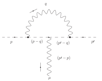
Figure 4: scalar-gauge field vertex.

$$\Gamma^{1}_{\mu}=-e^{2}\int\frac{d^{3}q}{(2\pi)^{3}}{(p+p^{\prime}-2q)_{\mu}(2p-q)_{\nu}(2p^{\prime}-q)_{\rho}G^{\nu\rho}(q)\over[(p-q)^{2}-m^{2}][(p^{\prime}-q)^{2}-m^{2}]}\,e^{-iq\times{\cal K}}e^{\frac{i}{2}p\times p^{\prime}},$$ (3)

where ${\cal K}_{\mu}\equiv(p^{\prime}-p)_{\mu}$. The above can be simplified to yield

$$\Gamma^{1}_{\mu}=-\frac{4e^{2}}{M}\int\frac{d^{3}q}{(2\pi)^{3}}{\epsilon^{\nu\rho\alpha}p_{\nu}{p^{\prime}}_{\rho}q_{\alpha}(p+p^{\prime}-2q)_{\mu}\over q^{2}[(p-q)^{2}-m^{2}][(p^{\prime}-q)^{2}-m^{2}]}\,e^{-iq\times{\cal K}}e^{\frac{i}{2}p\times p^{\prime}}.$$ (4)

The loop integral can be evaluated in the standard manner. After combining the denominators [we have used Eq. (26)] and shifting the integration variable we get

$$\Gamma^{1}_{\mu}=-\frac{8e^{2}}{M}\int_{0}^{1}dx\int_{0}^{x}dy\int\frac{d^{3}q}{(2\pi)^{3}}{\epsilon^{\nu\rho\alpha}p_{\nu}p^{\prime}_{\rho}{\tilde{q}}_{\alpha}[(2x-1)p_{\mu}+(1-2x+2y)p^{\prime}_{\mu}-2{\tilde{q}}_{\mu}]\over[{\tilde{q}}^{2}-\omega_{1}^{2}]^{3}}\,e^{-i{\tilde{q}}\times{\cal K}}e^{-\frac{i}{2}(1-2y)p\times p^{\prime}},$$ (5)

where $\omega_{1}^{2}=(1-y)^{2}m^{2}-(1-x)(x-y){\cal K}^{2}$ and $q={\bar{q}}+(x-y)p^{\prime}+(1-x)p$. For the sake of notational simplicity, we continue to denote the new integration variable ${\tilde{q}}$ as $q$ in this, as well as later calculations. In solving the above integrals, we retain only the $q_{\mu}q_{\alpha}$ term, since only this term gives magnetic moment type interaction. The momentum integral, using the result of Eq. (28), yields

$$\Gamma^{1}_{\mu}=-\frac{8ie^{2}\epsilon_{\mu\nu\rho}p^{\nu}{p^{\prime}}^{\rho}}{(2\sqrt{\pi})^{3}M}\int_{0}^{1}dx\int_{0}^{x}dye^{-\frac{i}{2}(1-2y)p\times p^{\prime}}\left[\frac{|{\widetilde{\cal K}}|}{2|\omega_{1}|}\right]^{1/2}K_{1/2}(|{\widetilde{\cal K}}||\omega_{1}|).$$ (6)

The parametric integrals can be handled in an elegant manner by going to a particular frame of reference: the rest frame of the scalar particle, where $p\times p^{\prime}=0$. Also, we take $\theta^{0i}=0$, since it is known that space-time noncommutativity violates unitarity mehen . Using

$$K_{\pm 1/2}(z)=\sqrt{\frac{\pi}{2}}\frac{e^{-z}}{\sqrt{z}},$$ (7)

and retaining terms first order in $\theta$ from the above expansion, we get

$$\Gamma^{1}_{\mu}=-{ie^{2}\epsilon_{\mu\nu\rho}{\cal P}^{\nu}{\cal K}^{\rho}\over 4\pi M}\left[\frac{1}{m}-\frac{|{\widetilde{\cal K}}|}{2}\right].$$ (8)

It must be mentioned that, the above expression is obtained in the ${\cal K}^{2}\rightarrow 0$ limit. Furthermore, we have replaced $p$ and $p^{\prime}$ using the relations for ${\cal K}_{\mu}$ and ${\cal P}_{\mu}={p^{\prime}}_{\mu}+p_{\mu}$.

III.2 Three-photon vertex contribution

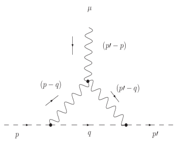
Figure 5: The three photon vertex contribution.

Here, we deal with the three-gluon contribution shown in Fig. (5), to the NC vertex:

$$\Gamma_{\mu}^{2} = -2ie^{2}M\int\frac{d^{3}q}{(2\pi)^{3}}{(p^{\prime}+q)_{\rho}(p-q)_{\lambda}G^{\nu\alpha}(p-q)\epsilon_{\alpha\mu\beta}G^{\beta\rho}(p^{\prime}-q)\over(q^{2}-m^{2})}\,\sin\left[{(p-q)\times(p^{\prime}-p)\over 2}\right]\,e^{\frac{i}{2}q\times{\cal K}},$$ (9)

$$= \frac{2ie^{2}}{M}\int\frac{d^{3}q}{(2\pi)^{3}}{\epsilon^{\nu\alpha\lambda}\epsilon_{\mu\alpha\beta}\epsilon^{\beta\rho\delta}(p^{\prime}+q)_{\rho}(p-q)_{\lambda}(p+q)_{\nu}(p^{\prime}-q)_{\delta}\over(q^{2}-m^{2})(p-q)^{2}(p^{\prime}-q)^{2}}\,\sin\left[{p\times p^{\prime}-q\times{\cal K}\over 2}\right]\,e^{\frac{i}{2}q\times{\cal K}}.$$

The above vertex $\Gamma_{\mu}^{2}$, can be written in terms of planar and non-planar contributions in the form,

$$\Gamma_{\mu}^{2}=\frac{4e^{2}}{M}\int\frac{d^{3}q}{(2\pi)^{3}}{\epsilon^{\nu\alpha\lambda}p_{\lambda}{p^{\prime}}_{\alpha}q_{\nu}q_{\mu}\over(q^{2}-m^{2})(p-q)^{2}(p^{\prime}-q)^{2}}[e^{\frac{i}{2}p\times p^{\prime}}-e^{-\frac{i}{2}p\times p^{\prime}}e^{iq\times{\cal K}}].$$ (10)

In obtaining the above expression, we have simplified the numerator using the standard $\epsilon$ manipulations. As before, combining the denominators and shifting the integration variable we get

$$\Gamma_{\mu}^{2}=\frac{8e^{2}}{M}\int^{1}_{0}dx\int^{x}_{0}dy\int\frac{d^{3}q}{(2\pi)^{3}}{\epsilon^{\nu\alpha\lambda}p_{\lambda}{p^{\prime}}_{\alpha}q_{\nu}q_{\mu}\over(q^{2}-\omega_{2}^{2})^{3}}\,[e^{\frac{i}{2}p\times p^{\prime}}-e^{iq\times{\cal K}}e^{\frac{i}{2}(1-2y)p\times p^{\prime}}],$$ (11)

where $\omega_{2}^{2}=m^{2}y^{2}-(x-y)(1-x){\cal K}^{2}$. The vertex can be separated as: $\Gamma_{\mu}^{2}=\Gamma_{\mu}^{2P}+\Gamma_{\mu}^{2NP}$. The planar part can be simplified:

$$\Gamma_{\mu}^{2P}=-\frac{ie^{2}}{4\pi M}\int_{0}^{1}dx\int_{0}^{x}dy\frac{\epsilon_{\mu\alpha\lambda}{p^{\prime}}^{\alpha}p^{\lambda}}{my}.$$ (12)

It can be noticed that the above planar contribution has a logarithmic divergence. The non-planar contribution can be written in the form

$$\Gamma_{\mu}^{2NP}=\frac{4ie^{2}\epsilon_{\nu\alpha\lambda}g^{\mu\nu}}{M(2\sqrt{\pi})^{3}}\int_{0}^{1}dx\int_{0}^{x}dy\left[\frac{|{\widetilde{\cal K}}|}{2|\omega_{2}|}\right]^{1/2}K_{1/2}(|{\widetilde{\cal K}}||\omega_{2}|).$$ (13)

On expanding the Bessel function and retaining contribution linear in the NC parameter, we see that the log divergence from the planar piece exactly cancels a similar divergence from the non-planar contribution. Hence, the 3-photon vertex is divergence free. Such a cancellation of divergences stemming from the planar and non-planar contributions has been noted in the photon self-energy calculation in 3+1 dimensions adas2 . The contribution to the vertex can be combined into a compact form:

$$\Gamma_{\mu}^{2}=\frac{ie^{2}}{4\pi M}\epsilon_{\mu\nu\rho}{{\cal P}}^{\nu}{{\cal K}}^{\rho}\frac{|{\widetilde{\cal K}}|}{4}.$$ (14)

III.3 Two-photon vertices

Figure 6: The two photon vertex.

Figure 7: The two photon vertex.

The two photon vertex amplitude in Fig. (7) can be written in the form

$$\Gamma_{\mu}^{3}=\frac{2e^{2}}{M}\int\frac{d^{3}q}{(2\pi)^{3}}{\epsilon^{\nu\rho\lambda}g_{\mu\nu}(2p^{\prime}-q)_{\rho}q_{\lambda}\over q^{2}[(p^{\prime}-q)^{2}-m^{2}]}\cos\left[\frac{q\times{\cal K}}{2}\right]e^{\frac{i}{2}p\times p^{\prime}}e^{-\frac{i}{2}q\times{\cal K}},$$ (15)

which yields,

$$\Gamma_{\mu}^{3}=\frac{2e^{2}}{M}\int_{0}^{1}dx\int\frac{d^{3}q}{(2\pi)^{3}}\frac{\epsilon_{\mu\rho\lambda}{p^{\prime}}^{\rho}q^{\lambda}}{(q^{2}-\omega_{3}^{2})^{2}}\left[e^{\frac{i}{2}p\times p^{\prime}}+e^{-iq\times{\cal K}}e^{-\frac{i}{2}(2x-1)p\times p^{\prime}}\right].$$ (16)

In obtaining the above expression we have redefined the integration variable by $q={\bar{q}}+xp^{\prime}$ and defined $\omega_{3}^{2}={p^{\prime}}^{2}x^{2}$. It is clear that the planar contribution is zero and only the non-planar integral survives:

$$\Gamma_{\mu}^{3NP}=\frac{2e^{2}\epsilon_{\mu\rho\lambda}{p^{\prime}}^{\rho}{\widetilde{\cal K}}^{\lambda}}{(2{\sqrt{\pi}}^{3})}\int_{0}^{1}dx\,e^{-\frac{i}{2}(2x-1)p\times p^{\prime}}\left[\frac{|{\widetilde{\cal K}}|}{2|\omega_{3}|}\right]^{-1/2}K_{-1/2}(|{\widetilde{\cal K}}||\omega_{3}|),$$ (17)

which in the rest frame gives the final answer in the form

$$\Gamma_{\mu}^{3NP}=\frac{e^{2}\epsilon_{\mu\nu\rho}{p^{\prime}}^{\nu}{\widetilde{\cal K}}^{\rho}}{4\pi M}\left[\frac{1}{|{\widetilde{\cal K}}|}-\frac{m}{2}\right].$$ (18)

In solving the momntum integral we have made use of the result from Eq. (27). Similarly for the other two photon vertex [Fig. (7)] we get,

$$\Gamma_{\mu}^{4NP}=-\frac{e^{2}\epsilon_{\mu\nu\rho}p^{\nu}{\widetilde{\cal K}}^{\rho}}{4\pi M}\left[\frac{1}{|{\widetilde{\cal K}}|}-\frac{m}{2}\right].$$ (19)

III.4 Two-photon and three-photon vertex

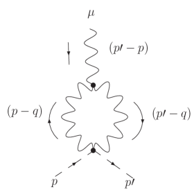
Figure 8: The two and three photon vertex.

This last subsection deals with the two photon and three gluon vertex. Similar to the contribution of Fig. (5) the contribution from this diagram is purely due to NC nature of the action. Calling the contribution from this diagram as $\Gamma_{\mu}^{5}$:

$$\Gamma_{\mu}^{5}=\frac{4ie^{2}}{M}\int\frac{d^{3}q}{(2\pi)^{3}}{g_{\alpha\beta}\epsilon^{\alpha\nu\lambda}\epsilon_{\mu\nu\rho}\epsilon^{\rho\beta\delta}(p^{\prime}-q)_{\delta}(p-q)_{\lambda}\over(p^{\prime}-q)^{2}(p-q)^{2}}\cos\left[\frac{(p^{\prime}-q)\times(p-q)}{2}\right]\sin\left[\frac{(p^{\prime}-p)\times(p^{\prime}-q)}{2}\right]e^{\frac{i}{2}p\times p^{\prime}}.$$ (20)

The standard manipulations give

$$\Gamma_{\mu}^{5}=-\frac{2ie^{2}}{M}\int\frac{d^{3}q}{(2\pi)^{3}}{\epsilon_{\mu\nu\lambda}\over(p^{\prime}-q)^{2}(p-q)^{2}}\left[\frac{{\cal P}^{\lambda}{\cal K}^{\nu}}{2}+{\cal K}^{\lambda}q^{\nu}\right]\sin[p\times p^{\prime}-q\times{\cal K}]e^{\frac{i}{2}p\times p^{\prime}}.$$ (21)

Proceeding as before we get

$$\Gamma_{\mu}^{5}=\frac{2ie^{2}}{M}\int_{0}^{1}dx\int\frac{d^{3}q}{(2\pi)^{3}}\frac{\epsilon_{\mu\nu\lambda}{\cal K}^{\lambda}q^{\nu}}{(q^{2}-\omega_{5}^{2})^{2}}\sin[q\times{\cal K}]e^{\frac{i}{2}p\times p^{\prime}},$$ (22)

where $\omega_{5}^{2}=x(x-1){\cal K}^{2}$. Performing the momentum integration, with $q={\bar{q}}+p+x{\cal K}$, one gets

$$\Gamma_{\mu}^{5}=-\frac{2e^{2}\epsilon_{\mu\nu\lambda}{\cal K}^{\lambda}{\widetilde{\cal K}}^{\nu}}{(2\sqrt{\pi})^{3}M}\int_{0}^{1}dx\left[\frac{|{\widetilde{\cal K}}|}{2|\omega_{5}^{2}|}\right]^{-1/2}K_{-1/2}(|{\widetilde{\cal K}}||\omega_{5}^{2}|)e^{\frac{i}{2}p\times p^{\prime}}.$$ (23)

Upon simplification, the contribution from this vertex diagram turns out to be

$$\Gamma_{\mu}^{5}=\frac{e^{2}\epsilon_{\mu\nu\rho}{\cal K}^{\nu}{\widetilde{\cal K}}^{\rho}}{4\pi M|{\widetilde{\cal K}}|}.$$ (24)

Combining the various vertices at first order in $\theta$, one gets

$$\Gamma_{\mu}=-{ie^{2}\epsilon_{\mu\nu\rho}{\cal P}^{\nu}{\cal K}^{\rho}\over 4\pi M}\left[\frac{1}{m}-\frac{3|{\widetilde{\cal K}}|}{4}\right]+\frac{e^{2}\epsilon_{\mu\nu\rho}{\cal K}^{\nu}{\widetilde{\cal K}}^{\rho}}{4\pi M}\left[\frac{2}{|{\widetilde{\cal K}}|}-\frac{m}{2}\right].$$ (25)

The above vertex contributions, as can be noticed, is separates into real and imaginary parts. The real part results due to the appearance of the $\theta$ dependent spin type term, unlike the other term where only the magnitude of $\theta$ appears. It can be seen from the above expression that, the theta independent term of the first piece arises due to the original vertex diagram which yielded a finite value to the parity odd part of the vertex function present in the commutative theory kogan1 . This parity odd term can couple to the external magnetic field and hence it was interpreted as the magnetic moment for the scalar particles. The present term receives a finite NC correction due to the appearance of non-planar integrals. This correction depends on the value of the NC parameter and hence can also be interpreted as a correction to the magnetic moment structure. The real piece of the vertex function is interesting because, the parity odd spin term couples not only to the external fields but it also couples to the NC parameter. Similar structures also arises in the angular momentum operator as has been shown recently mohrbach .

IV Conclusions

In conclusion, we have evaluated the NC vertex diagrams at one loop level, up to first order in $\theta$, for the scalar particles. The non-planar contributions brought in corrections to the spin structure and also coupled the external field to the $\theta$ tensor. It has been shown recently that, the magnetic moment for scalar matter fields in NC Maxwell-Chern-Simons can lead to the formation of bound states on plane ghosh . Hence, the implication of these loop corrections needs careful investigation. $\theta$ dependent contributions to angular momentum has been computed recently and has been related to Berry’s phase in momentum space. It is worth reminding that, in the conventional CS theory the Berry’s phase has manifested in the context of Hall effect. In this light, it will be exciting to study the NC contribution more carefully.

When the present manuscript was under preparation, we came across a preprint ajsilva , where the authors have analyzed the singularity structure of the vertex diagrams considered here.

Appendix A Important Integrals

Below we give the solutions of the various loop integrals encountered in the present work. For the sake of notational simplicity we denote ${\widetilde{\cal K}}^{\mu}\equiv\theta^{\mu\nu}{{\cal K}}_{\nu}$.

$$\frac{1}{ABC}=2\int^{1}_{0}dx\int^{x}_{0}dy\,[Ay+B(x-y)+C(1-x)]^{-3}.$$ (26)

$$\int\frac{d^{3}q}{(2\pi)^{3}}\frac{q_{\mu}}{[q^{2}-\omega^{2}]^{2}}\,e^{\pm iq\times{\cal K}}=\mp\frac{{\widetilde{\cal K}}_{\mu}}{(2\sqrt{\pi})^{3}}\left[\frac{|{\widetilde{\cal K}}|}{2|\omega|}\right]^{-1/2}\,K_{-1/2}(|{\widetilde{\cal K}}||\omega|).$$ (27)

$$\int\frac{d^{3}q}{(2\pi)^{3}}\frac{q_{\mu}q_{\nu}e^{\pm iq\times{\cal K}}}{[q^{2}-\omega^{2}]^{3}}=\frac{i}{(2\sqrt{\pi})^{3}}\left[\frac{{\widetilde{\cal K}}_{\mu}{\widetilde{\cal K}}_{\nu}}{4}\left[\frac{|{\widetilde{\cal K}}|}{2|\omega|}\right]^{-1/2}K_{-1/2}(|{\widetilde{\cal K}}||\omega|)-\frac{g_{\mu\nu}}{2}\left[\frac{|{\widetilde{\cal K}}|}{2|\omega|}\right]^{1/2}K_{1/2}(|{\widetilde{\cal K}}||\omega|)\right].$$ (28)

References

• (1) F. Wilczek, Magnetic flux, angular momentum, and statistics, Phys. Rev. Lett. 48 (1982) 1144; A. Goldhaber, Electromagnetism, spin, and statistics, Phys. Rev. Lett. 49 (1982) 905; F. Wilczek, Quantum mechanics of fractional-spin particles, Phys. Rev. Lett. 49 (1982) 957; H. J. Lipkin and M. Peshkin, Angular momentum paradoxes with solenoids and monopoles, Phys. Lett. B 118 (1982) 385; D. Arovas, J. R. Schrieffer and F. Wilczek, Fractional statistics and the quantum Hall effect, Phys. Rev. Lett. 53 (1984) 722; M. B. Paranjape, Induced angular momentum in (2+1)-dimensional QED, Phys. Rev. Lett. 55 (1985) 2390.
• (2) J. F. Schonfeld, A mass term for three-dimensional gauge fields, Nucl. Phys. B 185 (1981) 157; S. Deser, R. Jackiw and S. Templeton, Topologically massive gauge theories, Ann. Phys. 140 (1982) 372.
• (3) C. R. Hagen, A new gauge theory without an elementary photon, Ann. Phys. 157 (1983) 342; C. R. Hagen, Axial-gauge formulation of a three-dimensional field theory, Phys. Rev. D 31 (1985) 331; M. J. Bowick, D. Karabali and L. C. R. Wijewardhana, Fractional spin via canonical quantization of the O(3) nonlinear sigma model, Nucl. Phys. B 271 (1986) 417; C. H. Tze, Manifold splitting regularization, self-linking, twisting, writhing numbers of space-time ribbons and Polyakov’s Fermi-Bose transmutations, Int. J. Mod. Phys. A 3 (1988) 1959; G. W. Semenoff, Canonical quantum field theory with exotic statistics, Phys. Rev. Lett. 61 (1988) 517; P. K. Panigrahi, S. Roy and W. Scherer, Rotational anomaly and fractional Spin in the gauged CP1 nonlinear sigma model with the Chern-Simons term, Phys. Rev. Lett. 61 (1988) 2827; P. K. Panigrahi, S. Roy and W. Scherer, Canonical quantization of the interacting CP1 nonlinear sigma model with the Chern-Simons term, Phys. Rev. D 38 (1988) 3199.
• (4) A. M. Polyakov, Fermi-Bose transmutation induced by gauge fields, Mod. Phys. Lett. A 3 (1988) 325.
• (5) I. I. Kogan, Induced magnetic moment for anyons, Phys. Lett. B 262 (1991) 83; J. Stern, Topological action at a distance and the magnetic moment of point-like anyons, Phys. Lett. B 265 (1991) 119.
• (6) I. I. Kogan and G. W. Semenoff, Fractional spin, magnetic moment and the short-range interactions of anyons, Nucl. Phys. B 368 (1992) 718.
• (7) Y. Georgelin and J. C. Wallet, Anomalous magnetic moment for scalars and spinors in Maxwell-Chern-Simons electrodynamics, Phys. Rev. D 50 (1994) 6610.
• (8) C. Chou, V. P. Nair, and A. P. Polychronakos, On the electromagnetic interactions of anyons, Phys. Lett. B 304 (1993) 105; G. Gat and R. Ray, Anomalous magnetic moment of anyons, Phys. Lett. B 340 (1994) 162; M. Chaichian, W. F. Chen and V. Ya. Fainberg, On quantum corrections to Chern-Simons spinor electrodynamics, Eur. Phys. J. C 5 (1998) 545.
• (9) G. V. Dunne, Aspects of Chern-Simons theory, hep-th/9902115; A. Khare, Fractional statistics and Chern-Simons field theory in 2+1 dimenions, hep-th/9908027 and references therein.
• (10) M. Stone, Quantum Hall effect (World Scientific, Singapore, 1992) and references therein.
• (11) N. Seiberg and E. Witten, String theory and noncommutative geometry, JHEP 9901 (1999) 032.
• (12) H. S. Snyder, Quantized space-time, Phys. Rev. 71 (1947) 38.
• (13) J. Bellissard, A. van Elst and H. Schulz-Baldes, The non-commutative geometry of the quantum Hall effect, cond-mat/9411052.
• (14) L. Susskind, The quantum Hall fluid and non-commutative Chern-Simons theory, hep-th/0101029; A. P. Polychronakos, Quantum Hall states as matrix Chern-Simons theory, JHEP 0104 (2001) 011; B. Morariu and A. P. Polychronakos, Finite noncommutative Chern-Simons with a Wilson line and the quantum Hall effect, JHEP 0107 (2001) 006; S. Hellerman and M. Van Raamsdonk, Quantum Hall physics = noncommutative field theory, JHEP 10 (2001) 039; D. Karabali and B. Sakita, Orthogonal basis for the energy eigenfunctions of the Chern-Simons matrix model, Phys. Rev. B 65 (2002) 075304.
• (15) M. R. Douglas and N. A. Nekrasov, Noncommutative field theory, Rev. Mod. Phys. 73 (2001) 977; R. Jackiw, Physical instances of noncommuting coordinates, Nucl. Phys. Proc. Suppl. 108 (2002) 30; R. J. Szabo, Quantum field theory on noncommutative spaces, Phys. Rept. 378 (2003) 207; H. O. Girotti, Noncommutative quantum field theories, hep-th/0301237; R. J. Szabo, Magnetic backgrounds and noncommutative field theory, Int. J. Mod. Phys. A 19 (2004) 1837 and references therein.
• (16) A. N. Redlich, Parity violation and gauge noninvariance of the effective gauge field action in three dimensions, Phys. Rev. D 29 (1984) 2366; K. S. Babu, A. Das, and P. K. Panigrahi, Derivative expansion and the induced Chern-Simons term at finite temperature in 2+1 dimensions, Phys. Rev. D 36 (1987) 3725.
• (17) C.-S. Chu, Induced Chern-Simons and WZW action in noncommutative spacetime, Nucl. Phys. B 580 (2000) 352;
• (18) B. Chandrasekhar and P. K. Panigrahi, Finite temperature effects on the induced Chern-Simons term in noncommutative geometry, JHEP 0303 (2003) 015.
• (19) P. K. Panigrahi, R. Ray, and B. Sakita, Effective Lagrangian for a system of nonrelativistic fermions in 2+1 dimensions coupled to an electromagnetic field: Application to anyonic superconductors, Phys. Rev. B 42 (1990) 4036 and references therein.
• (20) A. A. Bichl, J. M. Grimstrup, V. Putz, and M. Schweda, Perturbative Chern-Simons theory on noncommutative R3, JHEP 07 (2000) 046.
• (21) A. Das and M. M. Sheikh-Jabbari, Absence of higher order corrections to noncommutative Chern-Simons coupling, JHEP 0106 (2001) 028.
• (22) C. P. Martin, Computing noncommutative Chern-Simons theory radiative corrections on the back of an envelope, Phys. Lett. B 515 (2001) 185.
• (23) G. H. Chen and Y. S. Wu, One-loop shift in noncommutative Chern-Simons coupling, Nucl. Phys. B 593 (2001) 562.
• (24) N. Grandi and G. A. Silva, Chern-Simons action in noncommutative space, Phys. Lett. B 507 (2001) 345.
• (25) D. Bak, K. Lee, and J. H. Park, Chern-Simons theories on the noncommutative plane, Phys. Rev. Lett. 87 (2001) 030402; V. P. Nair and A. P. Polychronakos, Level quantization for the noncommutative Chern-Simons theory, Phys. Rev. Lett. 87 (2001) 030403; M. M. Sheikh-Jabbari, A note on noncommutative Chern-Simons theories, Phys. Lett. B 510, (2001) 247.
• (26) The figures in this manuscript have been generated using JaxoDraw: D. Binosi and L. Theussl, JaxoDraw: A graphical user interface for drawing Feynman diagrams, Comput. Phys. Commun. 161 (2004) 76.
• (27) R. D. Pisarski and S. Rao, Topologically massive chromodynamics in the perturbative regime, Phys. Rev. D 32 (1985) 2081.
• (28) J. Gomis and T. Mehen, Space time noncommutative field theories and unitarity, Nucl. Phys. B 591 (2000) 265; O. Aharony, J. Gomis, and T. Mehen, On theories with light-like noncommutativity, JHEP 09 (2000) 023; N. Seiberg, L. Susskind, and N. Toumbas, Strings in background electric field, space/time noncommutativity and a new noncritical string theory, JHEP 06 (2000) 021; Space/time non-commutativity and causality, JHEP 06 (2000) 044; L. Alvarez-GaumΓ©, J. L. F. BarbΓ³n, and R. Zwicky, Remarks on time-space noncommutative field theories, JHEP 05 (2001) 057.
• (29) F. T. Brandt, A. Das, and J. Frenkel, General structure of the photon self-energy in noncommutative QED, Phys. Rev. D 65 (2002) 085017.
• (30) A. BΓ©rard and H. Mohrbach, Monopole and Berry phase in momentum space in noncommutative quantum mechanics, Phys. Rev. D 69 (2004) 127701.
• (31) S. Ghosh, Pauli term, anyons, ”Cooper pair”, …. or noncommutative Maxwell-Chern-Simons, hep-th/0407086.
• (32) E. A. Asano, L. C. T. Brito, M. Gomes, A. Yu. Petrov, and A. J. da Silva, Consistent interactions of the 2+1 dimensional noncommutative Chern-Simons field, hep-th/0410257.