DESY 04-214 November 12, 2004
HD-THEP-04-47

It is well-known that heterotic string compactifications have, in spite of their conceptual simplicity and aesthetic appeal, a serious problem with precision gauge coupling unification in the perturbative regime of string theory. Using both a duality-based and a field-theoretic definition of the boundary of the perturbative regime, we reevaluate the situation in a quantitative manner. We conclude that the simplest and most promising situations are those where some of the compactification radii are exceptionally large, corresponding to highly anisotropic orbifold models. Thus, one is led to consider constructions which are known to the effective field-theorist as higher-dimensional or orbifold grand unified theories (orbifold GUTs). In particular, if the discrete symmetry used to break the GUT group acts freely, a non-local breaking in the larger compact dimensions can be realized, leading to a precise gauge coupling unification as expected on the basis of the MSSM particle spectrum. Furthermore, a somewhat more model dependent but nevertheless very promising scenario arises if the GUT breaking is restricted to certain singular points within the manifold spanned by the larger compactification radii.

1 Introduction

Calabi-Yau or orbifold compactifications of the heterotic string [1] in its perturbative regime provide one of the most direct and beautiful paths from string theory to supersymmetric particle phenomenology [2, 3]. However, at the quantitative level, they are known to have serious problems related to the phenomenologically preferred not-so-small value of the unified gauge coupling and the values of Planck scale and Grand Unification scale [4]. Such difficulties may be avoided by appealing to threshold corrections reconciling $M_{GUT}$ with $M_{string}$ [5, 6] (see also [7, 8, 9] and, very recently, [10]). The problems may also be resolved in a regime where either the space-time or the world sheet expansion parameter of the string, or both, are not small [11, 12, 13]. However, the striking feature of quantitative gauge coupling unification in the minimal supersymmetric standard model (MSSM), which strongly supports the ideas of low-scale supersymmetry and thereby, indirectly, of the superstring, is in general lost.

In the present paper we approach the above set of problems focussing on new energy scales introduced in the compactification procedure. We analyse the issue of gauge coupling unification in heterotic orbifold models and conclude that the most promising constructions are those where the compact space is highly anisotropic, i.e. one or two of the 6 compactification radii are exceptionally large [11]. In other words, taking the empirical fact of precision gauge unification in the MSSM seriously (see [14] and refs. therein), one is forced into a regime that corresponds, from the low-energy perspective, to higher-dimensional grand unified theories (orbifold GUTs) [15, 16, 17, 18]. Possibilities for realizing such GUT models in explicit heterotic string constructions have recently been explored in [19, 20, 21] (for an earlier brief discussion see [22]).

To be more specific, we identify at least two interesting options for realizing precision gauge coupling unification. In both cases, this can be done in spite of possible non-perturbative stringy effects, which become relevant at the scale of the small compactification radii. In the first, conceptually simpler case, the geometry of the manifold defined by the large compactification radii is used to realize a non-local breaking of the GUT group. The corresponding compactification scale is the GUT scale, above which one enters a higher-dimensional field theory regime with a locally unbroken GUT symmetry. Any, possibly strongly coupled, string physics at or near the scale set by the small compactification radii does not influence gauge coupling unification which is, in fact, calculable within higher-dimensional field theory. The crucial technical point is that the GUT breaking has to be realized using a freely acting orbifold (see [23] for applications to non-local SUSY breaking and [24] for a recent field theoretic example with gauge symmetry breaking). A possible disadvantage of this scenario is that it may be difficult to find realistic models within this fairly constrained class of orbifold constructions. We consider this an interesting challenge for the future.

In the second, more familiar case, the GUT group is broken only at certain points within the space spanned by the large compactification radii. In spite of this local breaking, gauge unification at the level of one-loop precision can be maintained. This is the argument of “bulk dominance” familiar in the context of orbifold GUTs. From a stringy perspective this means that, even though the actual unification takes place in a regime that is hard to control quantitatively (small compactification radii near the string scale and/or large string coupling), the resulting uncalculable gauge coupling corrections are volume suppressed. Within this large volume (bulk) the GUT group is unbroken and strong coupling effects do not affect standard model (SM) gauge coupling differences. Such a scenario has the disadvantage that, in general, the logarithmic running of coupling differences continues above the compactification scale corresponding to the large radii [25, 16, 17]. This modified running depends on the details of the specific model and may significantly affect the prediction of low-energy gauge couplings. Thus, even though very promising concrete realizations are known in the field-theory context, extra assumptions beyond the simple use of the MSSM particle spectrum enter the analysis.

The paper is organized as follows. In Sect. 2 we attempt to make known arguments specifying the boundary of the weak-coupling regime of 10d heterotic string theory as quantitative as possible. This can be done by appealing to duality and identifying the point when massive states of the dual type I string or heterotic $M$ theory become lighter than the lowest massive heterotic string level. Alternatively, the same result is obtained by identifying the loop expansion parameter of the effective 10d gauge theory with the cutoff specified by the lowest-lying massive string state and requiring this parameter to be smaller than one. Writing the familiar ${\cal N}\!=\!1$ $d\!=\!10$ supergravity action at fixed dilaton VEV as

$$S=-\int d^{10}x\frac{\sqrt{G}}{(2\pi)^{7}g^{2}}\left(\frac{32}{{\alpha^{\prime}}^{4}}R+\frac{4}{{\alpha^{\prime}}^{3}}{\rm Tr_{V}}F_{\mu\nu}F^{\mu\nu}\right)\,,$$ (1)

we find that the dimensionless loop expansion parameter is $g^{2}$ and the theory is weakly coupled for $g<1$. Notice the presence of a large factor $(2\pi)^{7}$ in front of $g^{2}$. (The dilaton dependence is recovered by recalling that $g\sim\exp(\phi)$.)

Using this result and a network of dualities [26], we discuss in Sect. 3 the phenomenology of compactifications. We begin by quantifying the known difficulty of obtaining a realistic GUT from an isotropic heterotic string compactification. We then analyse the situation in anisotropic compactifications with one or two of the radii exceptionally large. Particular attention is paid to the question of how small the smaller radii can be made before perturbative control is completely lost. We emphasize the implications of T duality with Wilson lines and comment on the consequences of ${\cal N}\!=\!4$ or ${\cal N}\!=\!2$ supersymmetry in the 5 or 6d bulk.

We find that, for heterotic SO(32) string theory, a compactification with $d\!=\!2$ larger extra dimensions with inverse length set to the MSSM GUT scale $2\times 10^{16}$ GeV is possible. This implies the viability of a non-local GUT breaking scenario with correct breaking scale. In the $d\!=\!1$ case, such a non-local breaking scenario can not be realized. However, we find it possible to obtain a significant separation of 5d compactification scale and string scale allowing for an analysis in the framework of 5d orbifold GUTs. Similar studies are carried out in the $E_{8}\times E_{8}$ case, but the lack of $T$-duality on the $M$-theory side limits our power to control perturbativity. Using conservative estimates we find that, both in the $d\!=\!2$ and $d\!=\!1$ case, the large $M$-theory radius puts us in a phenomenologically more difficult situation than in the SO(32) case. Thus, heterotic SO(32) scenarios, which were neglected in the past and have only recently been subject to the attempt of a complete classification [28], may be favoured.

In Sect. 4, we describe explicitly how the various allowed compactification scales discussed above from a more formal perspective constrain the construction of realistic string GUTs. This analysis, which determines the main physical conclusions of the paper, reveals two main phenomenological options. These two options, both of which have already been briefly outlined above, correspond to non-local breaking in two extra dimensions (with radius set by the inverse GUT scale) and to local (fixed-point) breaking at singularities in one or two larger compact dimensions. Sect. 4.1 explains how to realize non-local GUT breaking in a heterotic orbifold construction and Sect. 4.2 provides a detailed analysis of mass scales in 5d models with local GUT breaking and large compactification radius (string-based orbifold GUTs). Amusingly, for $g\!=\!1$ and with the small radii set to the inverse string theory threshold, one finds a compactification scale $M_{c}\simeq 3.4\times 10^{16}\,{\rm GeV}$. (We are presently unable to make use of this intriguing proximity to the GUT scale in a realistic model).

Section 5 provides some illustrative concrete examples for the above scenarios. In particular, in Sect. 5.1 a simple $Z_{2}\times Z_{2}^{\prime}$ heterotic orbifold model is proposed which contains, at an intermediate energy scale, a 6d SO(10) gauge theory broken non-locally to a 4d Pati-Salam model using a freely acting discrete symmetry. Furthermore, Sect. 5.2 relates our discussion of models with local breaking to specific 5d orbifold GUTs and recent string theory models. Specifically, one can have $M_{c}\simeq 2.6\times 10^{15}$ GeV, with new string-theoretic states affecting the 5d field theory regime at about $20M_{c}$. This is marginally consistent with the concept of a 5d orbifold GUT.

Our conclusions are given in Sect. 6.

2 The weak coupling regime of the heterotic string

It is the purpose of this section to characterize the boundary of the perturbative regime of 10d heterotic string theory quantitatively. Although this is a familiar issue and the possible ways to achieve this are fairly obvious, we find it useful to include a detailed and hopefully self-contained discussion, where we carefully keep all relevant numerical coefficients. The results are crucial for the remainder of the paper since the potential loss of control of the stringy UV completion will be the main limiting factor in achieving realistic parameters in the low-energy field theory.

2.1 Field theory lagrangian and string parameters

The dynamics of heterotic string theory, at energies far below the mass of the first excited state, is described by the 10d supergravity plus super Yang-Mills lagrangian [1, 29]

$$S_{H}=-\int d^{10}x\sqrt{G_{H}}e^{-2\phi_{H}}\left(\frac{1}{2\kappa_{10}^{2}}R_{H}+\frac{1}{4\,g_{10}^{2}}{\rm Tr_{V}}F_{\mu\nu}F^{\mu\nu}\right)\,.$$ (2)

Here the trace ${\rm Tr_{V}}$ is taken in the vector representation of SO(32) and the field strength is defined by $F_{\mu\nu}=-i\,[D_{\mu},D_{\nu}]$ with $D_{\mu}=\partial_{\mu}+iA_{\mu}$. All fermionic and higher-dimension terms as well as the kinetic terms for the dilaton and 2-form field have been suppressed. Alternatively, the vector fields can also be defined to take values in the adjoint representation of SO(32), in which case one has to replace $\rm Tr_{V}$ with $(1/30){\rm Tr_{A}}$. This second form of the action then also describes the E${}_{8}\times$E₈ heterotic theory. Note that the restriction of the above lagrangian to a regular SU($N$) subgroup of either SO(32) or E${}_{8}\times$E₈ reads (with Minkowski metric and vanishing dilaton)

$${\cal L}\supset-\frac{1}{2\,g_{10}^{2}}{\rm Tr_{F}}F_{\mu\nu}F^{\mu\nu}\,,$$ (3)

where the trace is taken in the fundamental representation of SU($N$). Thus, for a compactification volume $V$, the conventional 4d GUT coupling (with phenomenological value $\sim 1/25$) is given by $\alpha_{\rm GUT}=g_{10}^{2}/(4\pi V)$.

The above action contains the two dimensionful parameters $\kappa_{10}$ and $g_{10}$, which are linked to the fundamental scale $\alpha^{\prime}_{H}$ of the underlying string theory by [1, 29] 

$$\frac{\kappa_{10}^{2}}{g^{2}_{10}}=\frac{{\alpha^{\prime}}_{H}}{4}\,.$$ (4)

Here we use standard conventions with a world sheet action $1/(4\pi\alpha^{\prime}_{H})\int d^{2}\sigma(\partial X)^{2}$, corresponding to a lowest-lying physical excited state with mass $m_{H}=2/\sqrt{{\alpha^{\prime}}_{H}}$.

The dimensionless ratio $u\equiv g_{10}^{4}/\kappa_{10}^{3}$ is not a true parameter of the theory since it can be changed by shifting $\phi_{H}$ by a constant and then redefining $g_{10}$ and $\kappa_{10}$ so that the form of Eq. (2) is not modified. This exercise also demonstrates that increasing the loop expansion parameter of string theory $g_{H}\sim\exp(\phi_{H})$ by a given factor is equivalent to increasing $u$ by the same factor. Thus, for any given vacuum of the heterotic string, we are free to choose conventions where $\phi_{H}=0$ and to use $g_{10}$ and $\kappa_{10}$ or, equivalently, $\alpha^{\prime}_{H}$ and $u$ as the unambiguous characteristics of this vacuum. The parameter $u$ then defines the strength of the string coupling.

Another perspective on the situation, which may be particularly natural for a low-energy field theorist, is the following. The gravitational and gauge parts of the action of Eq. (2) (with $\phi_{H}=0$) contain the two mass scales $\bar{M}_{P,10}$ and $M_{YM,10}$, defined by

$$\bar{M}_{P,10}^{8}=\frac{1}{\kappa_{10}^{2}}\,,\quad M_{YM,10}^{6}=\frac{1}{g_{10}^{2}},$$ (5)

which characterize the strong coupling regimes of the two respective field theories. On the one hand, a certain dimensionful combination of these two masses fixes, according to Eq. (4), the string scale. On the other hand, the dimensionless combination

$$u=\left(\frac{\bar{M}_{P,10}}{M_{YM,10}}\right)^{12}$$ (6)

determines the loop expansion parameter of the underlying string theory. Note that small heterotic string coupling corresponds to small 10d gauge coupling (measured in units of the 10d Planck mass).

Note that the numerical coefficient in the proportionality relation $u\sim g_{H}$ derived above is, at the moment, arbitrary (as is the coefficient in the relation $g_{H}\sim\exp(\phi)$.) In the following, we will characterize the perturbative regime directly in terms of $u$ and, after this is done, we will give a definition of $g_{H}$ in terms of $u$ such that, to the best of our knowledge, perturbation theory breaks down at the special point $g_{H}=1$. (It is this specific definition of a string coupling $g=g_{H}$ that appears in Eq. (1).)

In principle, it should be possible to define a more fundamental string loop expansion parameter in terms of the field (which differs from $\phi$ by an unknown constant) multiplying the Euler term in the world sheet action. This parameter would then directly measure the world sheet topology. In praxis, one starts in string perturbation theory by connecting the tree-level amplitude to field theory parameters. The one-loop amplitude is then related to the tree-level amplitude by a unitarity-based sewing procedure (see, e.g. [30]), and the relation to the Euler term of the world sheet action never arises. Comparing one-loop and tree-level terms one can then try to determine the field theory parameters characterizing the boundary of the perturbative regime and translate them into some (arbitrarily normalized) $g_{H}$. Conceptually, this is not very different from our approach based on the field-theoretically defined $u$. Of course, if one was given a number of non-trivial terms in the string-theoretic loop expansion of some physical quantity, a more trustworthy definition of perturbativity than the one we will offer could be obtained.

We finally note the useful expression

$$m_{H}=\bar{M}_{P,10}\,u^{1/4}$$ (7)

for the mass of the lowest-lying massive string state.

2.2 Duality criterion for weak coupling of SO(32)

One possibility to quantify the boundary of the weak coupling regime of the SO(32) heterotic string is to use the strong/weak coupling duality with type I string theory [31]. In analogy to Eq. (2), the relevant part of the low-energy action of the type I string reads

$$S_{I}=-\int d^{10}x\sqrt{G_{I}}\left(\frac{1}{2\kappa_{10}^{2}}e^{-2\phi_{I}}R_{I}+\frac{1}{4g_{10}^{2}}e^{-\phi_{I}}{\rm Tr_{V}}F_{\mu\nu}F^{\mu\nu}\right).$$ (8)

With the identifications $(G_{I})_{\mu\nu}=e^{-\phi_{H}}(G_{H})_{\mu\nu}$ and $\phi_{I}=-\phi_{H}$, Eqs. (2) and (8) describe the same field theory. Duality means that, for any given set of parameters of this Yang-Mills supergravity action, the two possible UV completions via heterotic or type I string theory are, in fact, identical.

The Regge slope $\alpha^{\prime}_{I}$ of the type I string relates to the world sheet action as in the heterotic case above. This implies that the first excited state has mass $m_{I}=1/\sqrt{{\alpha^{\prime}}_{I}}$ and the field theory parameters are related to $\alpha^{\prime}_{I}$ by [32, 33, 29]

$$\frac{g^{2}_{10}}{\kappa_{10}}=2\,(2\pi)^{\frac{7}{2}}{\alpha^{\prime}}_{I}.$$ (9)

We will describe the vacuum by $\phi_{H}=\phi_{I}=0$ such that Eqs. (2) and (8) take the same form and continue to use the parameters $M_{P,10}$, $M_{YM,10}$ as well as the parameter $u$ characterizing the strength of the string coupling: $g_{I}\sim 1/u$. The mass of the lowest-lying excited string state is then given, in terms of the field theory parameters, by

$$m_{I}=\bar{M}_{P,10}\,\sqrt{2}(2\pi)^{7/4}\,u^{-1/4}\,.$$ (10)

Now, comparing Eqs. (7) and (10), the following quantitative description of the weak and strong coupling regimes of the two string theories suggests itself. Taking, for example, $\bar{M}_{P,10}$ and $u$ as the fundamental parameters, focus first on the region where $u$ is very small and we can trust the perturbative heterotic description. According to Eqs. (7) and (10), in this regime $m_{H}\ll m_{I}$. This implies that the perturbative type I description has broken down since there exists a massive state much lighter than the first excited state of string perturbation theory. Next, focussing on the region of large $u$, where $m_{I}\ll m_{H}$ and we know that we can trust type I perturbation theory, the same argument can be made for the heterotic string: The heterotic perturbative description has broken down since the type I excited state with mass $m_{I}$ (which must be non-perturbative in nature from the heterotic perspective) is much lighter than the lowest-lying massive heterotic state. Finally, if one attempts to extend the heterotic and type I perturbative descriptions to larger/smaller $u$ respectively, one obviously faces a fundamental problem at the point where $m_{H}=m_{I}$ since, at this point, perturbative and non-perturbative states with comparable mass exist from both perspectives. It is then natural to define this special (critical) point

$$u_{c}^{2}=4(2\pi)^{7}$$ (11)

as the upper/lower boundary of the heterotic/type I perturbative regime.

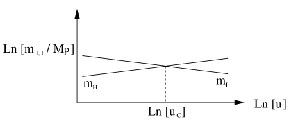
Figure 1: This figure shows $m_{H}$ and $m_{I}$ as functions of the coupling $u$ as defined by Eqs. (7) and (10). The critical point $u_{c}$ separates heterotic (left) and type I (right) weak coupling regimes.

This situation is illustrated in Fig. 1 where the masses of the lowest-lying heterotic and type I state are plotted as functions of $u$. Note that, on the basis of perturbation theory, one can only trust the lower of the two lines at any given point $u$. In particular, the extension of the $m_{I}$ curve into the region of small $u$ is, as far as we know, only speculative at the quantitative level. However, the extension of the $m_{H}$ curve into the region of large $u$ is known to be meaningful and to represent the heavy $D1$-brane of the type I theory [31].

As a cautionary remark, our characterization of the heterotic weak coupling regime by $u\ll u_{c}$ is certainly optimistic: We know that perturbation theory breaks down at $u=u_{c}$, but we can not exclude that it breaks down earlier. Note that so far we have only been concerned with perturbative calculability of the massive spectrum - the field theoretic gauge couplings will be discussed below.

2.3 Duality criterion for weak coupling of E${}_{8}\times$E₈

A similar analysis can be performed for the E${}_{8}\times$E₈ heterotic theory. The low-energy lagrangian of this theory is the same as in the SO(32) case, but the dual theory is now heterotic M-theory [34], i.e., an $S^{1}/Z_{2}$ orbifold reduction of 11d supergravity with gauge fields localized at the fixed points. The parameters $\kappa_{10}$ and $g_{10}$ of the resulting 10d Yang-Mills supergravity lagrangian (cf. Eq. (2) with $\phi_{H}=0$) are related by

$$\kappa_{10}^{2}=\frac{\kappa_{11}^{2}}{2\pi\rho}\qquad\mbox{and}\qquad g_{10}^{2}=2\pi(4\pi\kappa_{11}^{2})^{2/3}$$ (12)

to the 11d gravitational coupling $\kappa_{11}$ and the radius $\rho$ of the $S^{1}$. Note that, following [34], these relations assume compactification on an $S^{1}$ with $Z_{2}$ symmetry of the bulk fields (rather than compactification on an interval of size $\pi\rho$ with appropriate boundary conditions).

Although, in contrast to the type I string, this dual theory does not contain a microscopic description (i.e., an explicit UV completion), we can nevertheless repeat the strong/weak coupling argument of the last subsection. Indeed, since $\rho\sim u^{3/4}/\bar{M}_{P,10}$, we can trust the 11d field theory description at large $u$. This implies that the lowest-lying massive state in this regime is the first Kaluza-Klein (KK) excitation of supergravity with mass $m_{KK}=1/\rho$. In our definition of perturbativity this mass will take the place of $m_{I}$ in the last subsection. Thus, as before, we will assume that the E${}_{8}\times$E₈ heterotic string is weakly coupled as long as $m_{H}$ (the same as in the SO(32) theory) is smaller than $m_{KK}$. Explicitly, we have

$$m_{KK}=\bar{M}_{P,10}\,2(2\pi)^{7/2}\,u^{-3/4}\,,$$ (13)

which is illustrated in Fig. 2. Although Eq. (13) is very different from the analogous relation, Eq. (10), the critical point $m_{H}=m_{KK}$ lies, intriguingly, at exactly the same value of $u$, $u_{c}^{2}=4(2\pi)^{7}$, as in the SO(32) case.

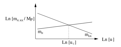
Figure 2: This figure shows $m_{H}$ and $m_{KK}$ as functions of the coupling $u$ as defined by Eqs. (7) and (13). The critical point $u_{c}$ separates heterotic-string (left) and 11d-supergravity (right) weak coupling regimes.

This motivates us to give a precise definition of a heterotic and a type I string coupling, $g_{H}$ and $g_{I}$,

$$g_{H}=\frac{1}{g_{I}}=\frac{u}{u_{c}}=\frac{1}{2(2\pi)^{7/2}}\left(\frac{\bar{M}_{P,10}}{M_{YM,10}}\right)^{12}\,.$$ (14)

These couplings relate in the usual way to the dilaton field, $g_{H}\sim\exp(\phi_{H})$, have a clear duality based definition in that $g_{H}=g_{I}=1$ characterizes the crossing points in Figs. 1 and 2, and will simplify subsequent formulae involving the 4d gauge coupling $\alpha_{GUT}$. Most importantly, with these definitions the usual perturbativity requirements $g_{H}<1$ and $g_{I}<1$ now have a more precise motivation in terms of the correctly predicted lowest-lying massive states.

2.4 Naive dimensional analysis in effective field theory

It is also possible to estimate the critical value of $u$, where string-theoretic perturbativity is lost, directly within the 10d low-energy effective field theory. More specifically, we will approximate the string-theoretic one-loop effect by the field-theoretic one-loop integral cut off at the string scale. Equivalently, we can take the point of view that the 10d gauge theory with cutoff $\Lambda$ has a dimensionless expansion parameter $\sim g_{10}^{2}\Lambda^{6}$ and require the cutoff (i.e. the string scale) to be sufficiently low to ensure that this expansion parameter is smaller than one.

To be generic, we begin with the Yang-Mills lagrangian in $d$ dimensions written in a representation $R$,

$${\cal L}_{YM}=-\frac{1}{4g^{2}_{d,R}}{\rm Tr_{R}}F_{\mu\nu}F^{\mu\nu}\,,$$ (15)

where the field strength is defined as after Eq. (2). On the basis of this lagrangian, the ratio of one-loop and tree-level terms (e.g., the one-loop correction to the gauge boson propagator) can be estimated as

$$\frac{\rm one\,\,loop}{\rm tree\,\,level}\,\simeq\,g_{d,R}^{2}\left(\frac{\Lambda^{d-4}}{(d\!-\!4)2^{d}\pi^{d/2}\Gamma(d/2)}\right)\,\left(\frac{C_{A}\,d(A)}{C_{R}\,d(R)}\right)\,.$$ (16)

Here the first factor $g_{d,R}^{2}$ is obvious, the second factor comes from the standard loop integral [36]

$$\int^{\Lambda}\frac{d^{d}k}{(2\pi)^{d}}\,\frac{1}{(k^{2})^{2}}\simeq\frac{1}{2^{d}\pi^{d/2}\Gamma(d/2)}\int_{0}^{\Lambda}|k|^{d-5}d|k|\simeq\frac{\Lambda^{d-4}}{(d\!-\!4)2^{d}\pi^{d/2}\Gamma(d/2)}\,,$$ (17)

while the last factor arises from the group-theoretic degeneracy of the gauge bosons propagating in the loop. It can be understood as follows (see, e.g., ref. [37] for group-theoretic details): The inverse propagator derived directly from Eq. (15) (without canonical field redefinition) comes with a factor $T_{R}$, defined by Tr${}_{R}({\bf T}_{a}{\bf T}_{b})=T_{R}\delta_{ab}$ for group generators ${\bf T}_{a},{\bf T}_{b}$. The 3-gauge-boson vertex comes with a factor $T_{R}f_{abc}$, where the structure constants are defined by $[{\bf T}_{a},{\bf T}_{b}]=if_{abc}{\bf T}_{c}$. Thus, the one-loop correction to a propagator, which contains two extra vertices and three extra propagators, has a relative group theory factor $C_{A}/T_{R}$, where $C_{A}$ is defined by $f_{abc}f_{dbc}=C_{A}\delta_{ad}$. (More generally, $C_{R}$ is the quadratic Casimir of the representation $R$, $({\bf T}_{a})_{ij}({\bf T}_{b})_{jk}=C_{R}\delta_{ik}$.) Using the identity $T_{R}\,d(A)=C_{R}\,d(R)$, where $d(A)$ and $d(R)$ are the dimensions of the adjoint representation and the representation $R$ respectively, one then finds the last factor in Eq. (16).

We would like to make some technical comments concerning this group-theoretical loop-factor: Clearly, we can not expect this “colour factor” to be exact – it is only meant to capture the dominant effect for large groups (e.g., the large $N$ limit of SU($N$)) and can be changed by an ${\cal O}(1)$ multiplicative constant if different conventions are chosen. In our conventions, the colour factor becomes trivial in the adjoint representation, which we consider a natural choice. Also, if we consider 4d SU($N$) with the lagrangian of Eq. (15) and $R=F$ the fundamental representation, the expansion parameter of Eq. (16) becomes $2g_{4,F}^{2}N/(16\pi^{2})$. In this case, the conventional gauge coupling used in phenomenology is defined as $g^{2}=2g_{4,F}^{2}$. Thus, the loop expansion parameter is equal to the ’t Hooft coupling $g^{2}N$ divided by the familiar 4d loop factor $16\pi^{2}$. For $N\!=\!3$, the expansion parameter is then $3\alpha_{s}/(4\pi)$, which is consistent with what is found in explicit QCD loop calculations.

Returning to the SO($N$) case relevant for the heterotic string, the colour factor appearing in Eq. (16) is $N\!-\!2$, i.e. 30 for SO(32). This is also the correct factor for E${}_{8}\times$E₈, as is obvious from the normalization factor (1/30) mentioned after Eq. (2) (which we now have effectively derived). Thus, with $d=10$ and $\Lambda=m_{H}$, the requirement that the loop factor of Eq. (16) is equal to one leads to a condition on $u$. The resulting critical value

$$u_{c}^{\prime 2}=\frac{3}{5}\cdot 2^{8}\cdot(2\pi)^{5}$$ (18)

is astonishingly close to that of Eq. (11), $u_{c}^{\prime 2}/u_{c}^{2}=48/(5\pi^{2})\simeq 0.97$. This should presumably not be taken too seriously, given that $\Lambda=m_{H}$ was an ad-hoc choice and that a small variation of the cutoff would affect the result significantly. Nevertheless, we view this subsection as an important confirmation that the critical coupling $u_{c}$ obtained before has the correct order of magnitude and that, with the above definition of the string coupling, $g_{H}<1$ is a useful criterion for perturbativity. We hope that this quantitative definition of the perturbative regime will also prove useful in other settings (cf. e.g. the discussion in [38]).

3 Isotropic vs. anisotropic compactifications

3.1 The isotropic case

As discussed in detail in [13], isotropic compactifications (with all the compactification radii roughly equal) do not straightforwardly lead to realistic unified models, neither in heterotic nor in type I string theory (with only $D9$-branes present). A crucial assumption made in this context is that the unification scale is linked to either the string or the compactification scale. The problems are due to the phenomenological requirement $\alpha_{GUT}\simeq 1/25$ together with the compactification formulas $\alpha_{GUT}=g_{10}^{2}/(4\pi V)$ and $M_{P}^{2}=8\pi\bar{M}_{P}^{2}=8\pi\bar{M}_{P,10}^{8}V$, with $M_{P}=1.22\times 10^{19}$ GeV. (We base our analysis on 1-loop MSSM running above an effective SUSY breaking scale $\sim m_{Z}$, leading to gauge coupling unification at $M_{GUT}\simeq 2\times 10^{16}$ GeV.)

To be specific, in a toroidal system with $V=(2\pi R)^{6}$, the gauge coupling is given by

$$\frac{\alpha_{GUT}}{2}=\frac{g_{H}^{2}}{(Rm_{H})^{6}}=\frac{g_{I}}{(Rm_{I})^{6}}\,,$$ (19)

with the string couplings defined in Eq. (14). Although written down in the oversimplified case of a torus, these equations can also be used to discuss the more general Calabi-Yau or orbifold case with typical length scale $R$. The above relations are to be supplemented with the formulae

$$M_{P}^{2}\frac{\alpha_{GUT}}{2}=m_{H}^{2}=g_{I}^{-1}m_{I}^{2}\,,$$ (20)

fixing the string scale in terms of the Planck scale and leading famously to the $g_{H}$-independent result $\alpha^{\prime-1/2}_{H}=8.6\times 10^{17}$ GeV in the heterotic case.

The unification scale problem is now very transparent. Focus first on the heterotic case and take the (arguably natural) radius $R\simeq m_{H}^{-1}$. The parametric smallness of $\alpha_{GUT}$ is then equivalent to a small string coupling $g_{H}$, which justifies quantitative gauge coupling unification, but at the too high scale $m_{H}$. In the type I case, we can analogously assume $R\simeq m_{I}^{-1}$, implying small $g_{I}$ and leading to the somewhat better but nevertheless high unification scale $m_{I}\simeq M_{P}\alpha_{GUT}/2\simeq 2.4\times 10^{17}$ GeV. Of course, we are using only the simplest form of heterotic-type I duality, considering type I theory with just $D9$-branes. This is a very restricted framework where the whole wealth of simple orbifold models of the heterotic theory is not available. One would then have to stick to the true Calabi-Yau case, which is difficult since the radius is too small to justify the supergravity approximation. Considering type I theory on its own, many interesting $D$-brane models can and have been considered. However, this goes beyond the scope of this work, which focusses on geometric constructions based directly on the 10d super Yang-Mills theory and its stringy UV completion.

The alternative point of view is to take $g_{H}=g_{I}=1$ and to derive the parametric smallness of $\alpha_{GUT}$ from a large compactification volume. This corresponds to identifying $M_{GUT}$ with $R^{-1}$. However, due to the high power of $R$ appearing in Eq. (19), the improvement is only minor: $R\simeq 2m_{H,I}$ is sufficient to explain the observed small gauge coupling so that the unification scale, if identified with $R^{-1}$, is not lowered significantly.

We would now like to comment on the heterotic M-theory case dual to the E${}_{8}\times$E₈ heterotic string. To discuss this case, Eqs. (19) and (20) have to be supplemented with the relation $\alpha_{GUT}/2=g_{H}^{-4}/(Rm_{KK})^{6}$ and $M_{P}^{2}\alpha_{GUT}/2=g_{H}^{2}m_{KK}^{2}$. In analogy to the heterotic and type I string theory discussion above, we can explain the smallness of $\alpha_{GUT}$ by either small $g_{H}^{-4}$ or large $R$. However, neither option leads to a sufficiently small GUT scale (if this scale is to be identified with $R^{-1}$). The interesting new possibility arising in the M-theory case is to take $R\ll m_{KK}^{-1}$ and $g_{H}^{-4}\ll 1$, which does indeed allow for solutions with $R^{-1}\ll M_{P}$. Nevertheless, limitations arise since the product space structure of 6d manifold and $S^{1}/Z_{2}$ assumed above is lost [11].

3.2 Taking some of the radii large

The possible solution to the above difficulties on which we now want to focus uses compactifications with very different radii such that the GUT scale is linked to the larger radii. As will be discussed below in explicit examples, this can be realized if the GUT group is broken by Wilson lines whose length is associated with those radii.

To be specific, consider heterotic models with internal space $T^{d}\times T^{6-d}$, where $T^{d}$ is symmetric with large radii $R_{l}$, and $T^{6-d}$ is symmetric with small radii $R_{s}$. Equation (19) is now replaced by

$$\frac{\alpha_{GUT}}{2}=\frac{g_{H}^{2}}{(R_{l}m_{H})^{d}(R_{s}m_{H})^{6-d}}\,.$$ (21)

As before, we use this simple toric situation as an approximation to the more interesting asymmetric Calabi-Yau or orbifold case.

The most favourable case of $d=1$ leads, for $g_{H}\simeq 1$ and $R_{s}\simeq m_{H}^{-1}$, to a GUT breaking scale $R_{l}^{-1}\simeq m_{H}/50\simeq 3.4\times 10^{16}$ GeV. In this situation, one is effectively considering a 5d theory in some intermediate energy range. To have a non-contractible Wilson line, this must be compactified to 4d on an $S^{1}$. Unfortunately, this situation can not be realized with Calabi-Yaus, which do not possess 1-cycles. It can also not be realized in the toric orbifold case since the $S^{1}$ compactification implies unbroken ${\cal N}\!=\!2$ SUSY in 4d. Thus, the lack of promising examples forces us to drop the $d=1$ case in this context.

The case $d=1$ remains interesting in the following sense: Even if $R_{l}$ is not the GUT scale, the relative logarithmic running of inverse SM gauge couplings could be different above $R^{-1}$ allowing the true GUT scale (where this differential running stops) to be changed. This occurs naturally in the context of 5d or 6d orbifold GUTs [16, 17]. Large threshold corrections producing such an effect where discussed early on in string model building [6]. Of course, such scenarios with modified differential running above the scale $R_{l}^{-1}$ can also be consider for $d>1$.

In the second best case of $d=2$, we will show explicitly below that, even at the simplest level of toric orbifolds, examples with 4d ${\cal N}\!=\!1$ SUSY and GUT-breaking Wilson lines associated with the two large radii exist. Numerically, the situation is clearly worse than for $d=1$, since $g_{H}\simeq 1$ and $R_{s}\simeq m_{H}^{-1}$ implies $R_{l}^{-1}\simeq m_{H}/7\simeq 2.5\times 10^{17}$ GeV. Alternatively, we can insist on $R_{l}^{-1}\simeq M_{GUT}$, implying the constraint $g_{H}/(R_{s}m_{H})^{2}\simeq 12$, which means that we have to face either small radii below the string length scale or a large string coupling.

3.3 Facing very small radii or a large string coupling

As argued above, we are led to consider string compactifications to $4+d$ dimensions where $R_{s}$ and $g_{H}$ are constrained by Eq. (21). We emphasize that, in this equation, $\alpha_{GUT}$, $m_{H}$ and $R_{l}$ are now fixed by phenomenology ($R_{l}^{-1}\simeq M_{GUT}$ in the simplest case but possibly varying depending on the details of the running). The interesting question is then how much quantitative control over this $4+d$ dimensional model we can gain and how much control we need in order to ensure quantitative gauge coupling unification. As already explained in the most promising case of $d=2$, the fully perturbative regime $g_{H}\ll 1$ and $R_{s}\gg m_{H}^{-1}$ is excluded.

The crucial point to be made in this subsection, which is also at the heart of the models with non-local GUT breaking discussed later on, is that we do not need a perturbative UV completion of the $4+d$ dimensional field theory. Specifically, in the case of $d=2$ and non-local GUT breaking, we only require control over light 6d states up to the scale $R_{l}^{-1}$. The contribution of all heavier states to non-universal GUT threshold corrections will be exponentially suppressed because of field theoretic locality. This is based on the fact that, on length-scales smaller than $R_{l}$ in the 6d field theory, the GUT group is never broken.

However, the absence of such dangerous light states is not entirely obvious. In particular, winding modes with mass $\sim R_{s}/\alpha^{\prime}$ are in general present. They become light in the limit of small $R_{s}$. This in itself would not be a very serious difficulty since, for $d=2$ and $g_{H}={\cal O}(1)$, small radii $R_{s}\simeq m_{H}^{-1}/\sqrt{12}$ are sufficient. Thus, the winding states are much heavier than $M_{GUT}$. The more serious issue is that these light states can spoil string-theoretic perturbativity. This can be quantified most easily by appealing to $T$ duality. In the simplest case, $T$ duality means that a physical setting with Regge slope $\alpha^{\prime}_{H}$, string coupling $g_{H}$, and a single compactification radius $R$ can be equivalently described by a string theory with parameters $\alpha^{\prime}_{H}$, $g^{\prime}_{H}=g_{H}\sqrt{\alpha^{\prime}}/R$ and compactification radius $R^{\prime}=\alpha^{\prime}/R$ [39]. The above light winding states are the KK states of the dual description. The real problem is the potentially very large dual string coupling that arises if the duality is applied to all small radii. This strongly coupled theory may contain extremely light non-perturbative states.

Before entering a more detailed discussion of specific settings, we have to recall that we used and will continue to use tree level formulae in our coupling strength analysis. This is justified if the intermediate-energy $4\!+\!d$ dimensional theory has maximal (${\cal N}=4)$ SUSY protecting us from loop corrections and if we can appeal to bulk dominance (parametrical largeness of the $4\!+\!d$ dimensional volume) in the last compactification step. If, at the intermediate stage, we encounter a higher-dimensional ${\cal N}=2$ gauge theory, ${\cal O}(1)$ corrections to the gauge coupling may arise. We ignore them with the argument that, at the present level of precision, all that matters is the approximate size of the underlying string coupling and not the specific ${\cal O}(1)$ factor linking it to the GUT gauge coupling. However, it is conceivable that in very specific settings, e.g. in situations close to the UV fixed point regime of [40], the 1-loop corrections of the ${\cal N}=2$ SUSY gauge theory modify the naive tree-level analysis dramatically and allow for a solution of the string scale/GUT scale problem very different from the one discussed in this paper.

3.3.1 Two large and four small radii

The potential problem of dangerous light states can be brought under control if, using a network of dualities [26], we manage to find a perturbative UV completion in the simplified case of a flat $4\!+\!d$ dimensional theory. This may be possible by going to the type I description via $S$ duality. We now focus on $d=2$. Consider the two-dimensional space parameterized by $g_{H}$ and $R_{s}$ and enforce the constraint

$$g_{H}=12(R_{s}m_{H})^{2}\,.$$ (22)

This defines a one-parameter set of models within which we can search for an appropriate dual description of our 6d low-energy theory. The type I duals have parameters $g_{I}=g_{H}^{-1}$ and $m_{I}=g_{H}^{-1/2}m_{H}$. Unfortunately, we immediately find $R_{s}m_{I}\simeq 1/\sqrt{12}$, i.e., we have the problem of too small radii. Notice that the product of dual string scale and small radius does not depend on the choice of parameters in the original heterotic model. This is a special feature of the case $d=2$. Next, we $T$-dualize the type I model. The resulting $T$-dual type IIB theory has coupling $g_{II}=g_{I}\alpha_{I}^{\prime 2}/R_{s}^{4}$, radii $R_{s}^{\prime}=\alpha_{I}^{\prime}/R_{s}$ and gauge fields localized on $D5$-branes [41]. Writing this in terms of the original parameters and expressing $R_{s}$ as a function of $g_{H}$ and $m_{H}$, one finds

$$g_{II}\simeq(12)^{2}g_{H}^{-1}\qquad\mbox{and}\qquad R_{s}^{\prime}\simeq\frac{\sqrt{12g_{H}}}{m_{H}}\,.$$ (23)

Using $g_{H}\simeq(12)^{2}$ to keep $g_{II}$ at the boundary of perturbativity, this implies $R_{l}/R_{s}^{\prime}\simeq 2$, i.e., the KK states of this (almost) perturbatively controlled model are marginally above the GUT-breaking scale. Notice that all other string states (e.g., the fundamental string excitations with mass $m_{I}$) are heavier than these KK states and are therefore less problematic.

Of course, we do not really need the type II model with coupling $g_{II}$ to be perturbative. Our interest is only in the light states of mass $R_{s}^{\prime-1}$. We can therefore go to smaller $g_{H}$, hoping that Eq. (23) remains qualitatively valid and the dangerous light states become heavier. The most we can do is to take $g_{H}\simeq 48$ since, going to even smaller $g_{H}$, the coupling $g_{H}^{\prime}$ of the heterotic $T$ dual becomes larger, $g_{H}^{\prime}>g_{H}$ (using the constraint Eq. (22)). Equation (23), if taken seriously, then implies $R_{l}/R_{s}^{\prime}\simeq 3.5$.

The presence of the light (a factor of 2 to 3 above $R_{l}^{-1}$) non-perturbative states found above is potentially dangerous. However, since they are Kaluza-Klein excitations in the internal dimensions orthogonal to the $D5$-branes, they are not charged under the gauge group. We can therefore hope that their sole effect will be a mild modification of the internal geometry, not affecting the basic picture of field-theoretic non-local GUT breaking at $M_{GUT}\simeq R_{l}^{-1}$. Furthermore, since field-theoretic locality leads to an exponential suppression of all effects related to states above the scale $R_{l}^{-1}$, we can hope that the very mild hierarchy $R_{l}/R_{s}^{\prime}$ found above is sufficient.

In many concrete models, the situation will be further improved by the following effect. In the presence of Wilson lines, which are anyway a crucial ingredient in realistic model building, the toroidal dimensional reduction [42] and, consequently, the T-duality rules [43] are modified, with the effect that the potential perturbativity loss can be avoided.

Specifically, in a model with $g_{H}<1$ and $R_{s}<{\alpha^{\prime}}_{H}^{1/2}$, the potential loss of calculability is due to the light winding modes of mass $m\sim R_{s}/{\alpha^{\prime}}_{H}$. The presence of a Wilson line $A$ modifies the relevant mass formula. Focussing for simplicity on the case of one compact dimension, the masses of states in a gauge representation labelled by the root-space vector $q$ read [42, 29]

$$m^{2}=\left[\frac{n}{R}-q\cdot A-wR\left(\frac{1}{{\alpha^{\prime}}_{H}}+\frac{A\cdot A}{2}\right)\right]^{2}+\frac{4\tilde{N}}{\alpha^{\prime}_{H}}\,.$$ (24)

Here the dot-product refers to vector multiplication in root space and the integers $n$ and $w$ are the KK and winding numbers, which are subject to the constraint

$$nw=1-N+\tilde{N}-\frac{1}{2}\,q\cdot q\,.$$ (25)

The non-negative integers $N$ and $\tilde{N}$ characterize the excitation levels of the left-moving world-sheet bosons and the right-moving Ramond sector respectively.

The crucial point following from the above equations is that, for a moderately large Wilson line value, the tower of light winding modes with spacing $R/\alpha^{\prime}_{H}$ disappears. At least naively, this seems to solve the problem completely. From a duality point of view this is also apparent since the modification of the $T$-duality rules [43] is such that the $T$-dual theory has a smaller coupling than without Wilson lines. As a result, we can expect that potentially dangerous non-perturbative states, whose mass grows with the inverse coupling, become heavier.

3.3.2 One large and five small radii

As already explained, the analysis is very sensitive to the number of large compact dimensions. For $d>2$ the situation is qualitatively similar to the $d=2$ case but, clearly, the potential perturbativity loss is more severe. We do not enter into a numerical discussion of these cases. The case $d=1$, instead, deserves more care. Indeed, even though we know that a single large internal dimension cannot be used to set the scale of non-local GUT breaking, it can provide low-scale thresholds which can be relevant for the GUT scale/string scale problem.

Therefore, in the following discussion of the $d=1$ case, we do not set $R_{l}^{-1}$ equal to $M_{GUT}$ but keep it as a free parameter. We are thus studying a space parameterized by $R_{l}$, $R_{s}$ and $g_{H}$ with the constraint

$$\frac{\alpha_{GUT}}{2}=\frac{g_{H}^{2}}{(R_{l}m_{H})(R_{s}m_{H})^{5}}\,,$$ (26)

which provides us with a two-parameter set of models. We parameterize this set by $R_{l}$ and $R_{s}$. As long as $R_{l}<50/m_{H}$, we can choose $R_{s}\simeq m_{H}^{-1}$ and find ourselves in the perturbative heterotic regime. This puts the lowest-lying massive states of the 5d field theory at the scale $m_{H}$. If, however, $R_{l}>50/m_{H}$, the heterotic UV completion becomes non-perturbative.

In this case, we can try the type I dual with $g_{I}=g_{H}^{-1}$ and $m_{I}=g_{I}^{1/2}m_{H}$. One finds

$$(R_{s}m_{I})\,g_{I}^{-1/10}\simeq\left(\frac{50}{R_{l}m_{H}}\right)^{1/5}\,,$$ (27)

implying that this description is also non-perturbative (either $g_{I}^{-1}$ or $R_{s}m_{I}$ have to be smaller than one). The $T$ dual of this type I model, which is a type IIA model with $D4$-branes, has parameters

$$R_{s}^{\prime}=\frac{\alpha^{\prime}_{I}}{R_{s}}\simeq\frac{R_{l}}{7}\frac{(R_{s}m_{H})^{3/2}}{(R_{l}m_{H})^{1/2}}\qquad\mbox{and}\qquad g_{II}=\frac{g_{I}}{(m_{I}R_{s})^{5}}=\frac{(R_{l}m_{H}/50)^{3/4}}{(R_{s}m_{H})^{5/4}}\,,$$ (28)

which finally provides a perturbative UV completion. More specifically, we can go to the boundary of the perturbative domain, $g_{II}\simeq 1$, by choosing $R_{s}$ such that

$$(R_{s}m_{H})^{5/4}\simeq(R_{l}m_{H}/50)^{3/4}\,.$$ (29)

This implies

$$R_{s}^{\prime}\simeq\frac{R_{l}}{50}\left(\frac{R_{l}m_{H}}{50}\right)^{2/5}\simeq m_{I}^{-1}\left(\frac{R_{l}m_{H}}{50}\right)^{2/5}\,,$$ (30)

so that, from a 5d field theory perspective, the lowest-lying massive states appear at a scale $50M_{c}$ in the best case. As will be discussed in more detail in Sect. 4.2, this validity range of the 5d field theory is sufficient for quantitative gauge coupling unification in the orbifold GUT framework. However, $R_{l}$ can not be made much larger than $50/m_{H}$ without restricting the above validity range. (The second part of Eq. (30) confirms that there is no danger from too small radii in the type IIA model.)

3.3.3 Large and small radii in the E${}_{8}\times$E₈ theory

In the case of the heterotic E${}_{8}\times$E₈ theory, we have less control than in the SO(32) case discussed above. The reason is that, after using the analogue of $S$ duality to go to the $M$ theory (11d supergravity on $S^{1}/Z_{2}$) side of the model, we do not have the tool of $T$ duality at our disposal. It is then difficult to quantify the danger of making the small radii $R_{s}$ too small. We attempt to achieve this in the following way.

From the formulae of Sect. (3.1) one derives the $S^{1}$ radius

$$\rho=\sqrt{R_{l}^{d}R_{s}^{6-d}}\,\frac{m_{H}^{2}}{7}\,,$$ (31)

with $m_{H}=2/\sqrt{{\alpha^{\prime}}_{H}}=2\times 8.6\times 10^{17}$ GeV being fixed phenomenologically. To proceed, we start from the ‘critical point’ $g_{H}=1$, where we assume both the heterotic string and the $M$ theory description to be qualitatively correct. At this point, we set the small radii to the minimal value suggested by the string theory description, $R_{s}\simeq m_{H}^{-1}$. We then find $\rho\simeq R_{l}/7\simeq m_{H}^{-1}$ for $d=2$ and $\rho\simeq R_{l}/50\simeq m_{H}^{-1}$ for $d=1$.

Now we want to see whether we can make $R_{l}$ larger, which corresponds to moving into the $M$ theory regime. We assume that the smallness of $R_{s}$ is limited by physics local in the 11th dimension (i.e., we are not allowed to make $R_{s}$ too small in units of $g_{10}^{1/3}$ or $\kappa_{11}^{2/7}$). Thus, when moving away from $g_{H}=1$ the small radii, if kept at their minimal value, scale as

$$R_{s}\sim g_{10}^{1/3}\sim(R_{l}^{d}R_{s}^{6-d})^{1/6}\,,$$ (32)

where the second proportionality follows from the phenomenologically fixed 4d gauge coupling. The above implies $R_{s}\sim R_{l}$ so that, on the basis of Eq. (31), the parameter $\rho$ grows like $R_{l}^{3}$ if $R_{l}$ is increased above its critical value (i.e., its value at $g_{H}=1$ and minimal $R_{s}$). From the low-energy field theory perspective, this means that the threshold set by $\rho$ (and thus the potentially non-perturbative physics related to the interplay of the curved branes and the bulk) move quickly into the infrared if we attempt to take $R_{l}$ to or below the GUT scale.

Numerically, for $d=2$ the ratio of small and large radii is fixed to $R_{s}/R_{l}\simeq 1/7$. The relation

$$\rho\simeq\frac{R_{l}}{7}\left(\frac{R_{l}m_{H}}{7}\right)^{2},$$ (33)

then implies that, when $R_{l}$ is increased, one encounters the equality $R_{l}=\rho$ already at $R_{l}^{-1}\simeq 9.3\times 10^{16}$ GeV. Thus, it is impossible to reach the GUT scale without leaving the 6d gauge theory regime (although the mismatch is not too severe).

In the $d=1$ case, instead, the ratio of radii is fixed at $R_{s}/R_{l}\simeq 1/50$ and the $M$ theory radius is given by

$$\rho\simeq\frac{R_{l}}{50}\left(\frac{R_{l}m_{H}}{50}\right)^{2}\,.$$ (34)

The large power of $R_{l}$ on the r.h. side makes the situation less favourable than in the SO(32) case, where an analogous relation is given by the first part of Eq. (30). For example, $\rho=R_{l}$ implies $R_{l}^{-1}\simeq 4.8\times 10^{15}$ GeV, meaning that there is no 5d field theory regime below that scale. Even with $R_{l}^{-1}\simeq M_{GUT}$ and the resulting cutoff $\rho^{-1}\simeq 3.5\times 10^{17}$ GeV the validity range of 5d field theory is still relatively small (a factor $\sim 17$ in energy scales).

In both cases, the constraints on low values of $R_{l}^{-1}$ and a corresponding higher-dimensional field theory at low energy scales are more severe than for the SO(32) heterotic string. However, our analysis was conservative: larger $R_{l}$ might be feasible if, for example, $R_{s}$ could be taken to values below $m_{H}^{-1}$ (recall that this appears to be possible in the SO(32) case because of the modified $T$ duality in the presence of Wilson lines). We discuss in 5.2 the relevance of these bounds on heterotic $E_{8}\times E_{8}$ orbifold GUT model building.

4 Non-local vs. local gauge symmetry breaking in string theory

4.1 Non-local breaking on a freely-acting orbifold

Orbifold compactifications of string theory allow for many gauge and SUSY breaking patterns which can be classified using the concept of “locality”. We will call the breaking of a certain symmetry in an extra-dimensional model “local” if it is realized at certain points in the internal space; it is instead “non-local” if it is due to some global property of the whole internal space. In the first case, the scale of breaking is tied to the cutoff, e.g., the string scale. In the second case, it is related to the size of the internal space.

A standard example of local gauge symmetry and SUSY breaking is the quantization on an orbifold generated by a discrete symmetry $g$ which acts as a rotation in the internal space, combined with a non-trivial transformation of the gauge bundle. The breaking is local since there are, in the internal space, points $x_{f}$ such that $g\,:\,x_{f}\to x_{f}$. The gauge symmetry and SUSY breaking is localized in these fixed points. Furthermore, the twisted states, which come in multiplets of the reduced gauge symmetry (SUSY) and do not fill out multiplets of the original symmetry, live at these points.

Non-local breaking can instead be realized by modding out a discrete symmetry generated by an operator $h$ which acts freely (i.e., without fixed points) in the internal space. In this case the symmetry breaking due to $h$ is not localized and the breaking scale is not tied to the string scale. Instead, it is set by some of the compact radii (cf. Sect. 5.1). For example, defining $h$ as a translation in the internal space, combined with a rotation in the gauge (R-symmetry) group, a non-local gauge symmetry (SUSY) breaking can be realized. This mechanism is also known as Scherk-Schwarz symmetry breaking [44] or Hosotani mechanism [45] (cf. also [2, 46]). We emphasize that our interest will be in the quantized, non-local realization of gauge symmetry breaking [46] (see also [47] and refs. therein) rather than in the continuously varying Wilson lines usually associated with the term Hosotani-mechanism. String-theoretic implementations following [44] focussed mainly on SUSY breaking [48]. They were later realized in explicit orbifold constructions [49] and further developed both in heterotic [50] and type I model building [51].

It is possible to use the non-local mechanism to break a GUT gauge group to the SM at an energy scale different from the string scale, solving, in this way, the string scale/GUT scale problem. The main idea is to build an orbifold model where the orbifold group contains non-freely acting operators $g^{\prime}$, preserving the GUT symmetry, and freely acting operators $g$, breaking the GUT symmetry [46]. Of course, by this orbifolding, an appropriate SUSY breaking to ${\cal N}=1$ in 4d must also be realized.

	$\{g^{\prime}\}$		$\{g\}$
$\mathcal{N}=4$ SO(32) or E${}_{8}\times$E8	$\longrightarrow$	$\mathcal{N}=*$ $\mathcal{G}_{GUT}\times\mathcal{G}$	$\longrightarrow$	$\mathcal{N}=1$ $\mathcal{G}_{SM}\times\mathcal{G^{\prime}}$

To be more specific, we consider the internal space $T^{6}=T^{2}\times T^{2}\times T^{2}$, with each of the 2-tori parameterized by a complex number $z_{i}$, $i=1,\,2,\,3$. The torus structure emerges after the identifications $z_{i}\sim z_{i}+(n+m\tau_{i})$, $\tau_{i}$ being the complex structure moduli of the 2-tori and $n,\,m\,\in\,\mathbb{Z}$.

Now introduce a group $Z_{N}\times Z^{\prime}_{M}$ with generators $g$ and $g^{\prime}$. Let $g$ act as a translation in one of the 6 compact dimensions, e.g.,

$$g:\mbox{Re}(z_{1})\rightarrow\mbox{Re}(z_{1})+a\,,$$ (35)

while the action in the rest of the space is generic. The full action of $g$ is then free and we can embed $g$ in the gauge group in a GUT-symmetry-breaking way. Notice that, as discussed earlier, $g$ breaks SUSY to $\mathcal{N}\geq 2$ (or to $\mathcal{N}=0$, which is not interesting in our context). Thus, we clearly need an extra orbifold operator $g^{\prime}$ generating the second $Z^{\prime}_{M}$. We do not require $g^{\prime}$ to act freely which means that, to have non-local GUT-breaking, the gauge embedding of $g^{\prime}$ must be GUT-preserving. In order to reduce SUSY to $\mathcal{N}=1$ in 4d, it is necessary that $g^{\prime}$ contains a rotation involving Re$(z_{1})$. Furthermore, given the non-free action of $g^{\prime}$, the other GUT-breaking operators $g^{a}\cdot{g^{\prime}}^{b}$ ($a,b\in\{0,\cdots,N\!-\!1\}$, $a\neq 0$) act, in general, non-freely. This can be avoided by a careful choice of the actions of $g$ and $g^{\prime}$ in the rest of the internal dimensions. Remarkably, these actions can not be just standard rotations around the origin.

We now provide two simple examples for $N=M=2$ and for $N=M=3$, leaving a complete classification of this type of orbifold models for future work. In the first case we choose

$$g:z_{1}\rightarrow z_{1}+\frac{1}{2},\hskip 17.07182ptg:z_{2}\rightarrow-z_{2},\hskip 45.52458ptg:z_{3}\rightarrow-z_{3},\,\,\,\,\,\mbox{GUT-breaking;}$$ (36)

$$g^{\prime}:z_{1}\rightarrow-z_{1},\hskip 28.45274ptg^{\prime}:z_{2}\rightarrow-z_{2}+\frac{1}{2},\hskip 19.91684ptg^{\prime}:z_{3}\rightarrow z_{3},\,\,\,\,\,\,\mbox{GUT-preserving.}$$ (37)

Note that the GUT-breaking operator $g$ acts as a rototranslation. It is easy to check that the second GUT-breaking operator $g\cdot{g^{\prime}}$ also acts freely (the key being that the action of $g^{\prime}$ on the second torus is not just a rotation around the origin). The breaking is delocalized along the real parts of $z_{1}$ and $z_{2}$. In the limit where the two corresponding radii become large, one recovers the 6d field theory model of [24]. (The underlying non-trivial 2d topology, which is that of the projective plane, has been mentioned before in the non-SUSY context [52].)

In the second case, since we have $Z_{3}$-rotations, we need $\tau_{i}=e^{\pi i/3}$. We choose

$$g:z_{1}\rightarrow z_{1}+\frac{\tau+1}{3},\hskip 8.5359ptg:z_{2}\rightarrow e^{2\pi i/3}z_{2},\hskip 62.59596ptg:z_{3}\rightarrow e^{-2\pi i/3}z_{3};$$ (38)

$$g^{\prime}:z_{1}\rightarrow e^{4\pi i/3}z_{1},\hskip 22.76228ptg^{\prime}:z_{2}\rightarrow e^{-2\pi i/3}z_{2}+\frac{\tau+1}{3},\hskip 9.38945ptg^{\prime}:z_{3}\rightarrow e^{-2\pi i/3}z_{3}+\frac{\tau+1}{3}.$$ (39)

As before, $g$ is GUT-breaking and $g^{\prime}$ is GUT-preserving.

It is interesting to study the relation of these kinds of models to constructions with gauge symmetry breaking by Wilson lines, both in the continuous and quantized case. Models with quantized Wilson lines are conceptually close to our discussion since a quantized Wilson line is obtained if a freely acting symmetry $h^{\prime}$ (a translation in the internal space) combined with a (quantized) rotation in the gauge bundle is modded out. The quantization arises from the consistency with other (rotational) symmetries modded out in parallel. As we will demonstrate below, our non-local breaking can be realized, quite analogously, by consistently combining Wilson lines with orbifold operations. However, in our case the latter can not be merely standard rotations. Rather, they must include rototranslations.

To make the above discussion more explicit, consider the following $Z_{2}\times Z^{\prime}_{2}\times Z^{\prime\prime}_{2}$ example, where the various factors of the orbifold group are generated by $g$, $g^{\prime}$ and $g^{\prime\prime}$,

$$g:z_{1}\rightarrow z_{1}+\frac{1}{2}\,,\hskip 17.07182ptg:z_{2}\rightarrow z_{2}\,,\hskip 45.52458ptg:z_{3}\rightarrow z_{3}\,,$$ (40)

$$g^{\prime}:z_{1}\rightarrow z_{1}\,,\hskip 36.98866ptg^{\prime}:z_{2}\rightarrow-z_{2}+\frac{1}{2}\,,\hskip 12.23447ptg^{\prime}:z_{3}\rightarrow-z_{3}\,,$$ (41)

$$g^{\prime\prime}:z_{1}\rightarrow-z_{1}\,,\hskip 24.75375ptg^{\prime\prime}:z_{2}\rightarrow-z_{2}\,,\hskip 33.57404ptg^{\prime\prime}:z_{3}\rightarrow z_{3}+\frac{1}{2}\,.$$ (42)

We choose the actions of $g^{\prime}$ and $g^{\prime\prime}$ in the gauge bundle to be GUT-preserving while that of $g$ is GUT-breaking. Actually, the GUT-breaking operator $g$ is nothing else than a quantized Wilson line. However, in general this is not sufficient to make the overall GUT breaking non-local. All the other GUT-breaking operators, $g\cdot g^{\prime}$, $g\cdot g^{\prime\prime}$, and $g\cdot g^{\prime}\cdot g^{\prime\prime}$, have to act freely as well. For this it is crucial that $g^{\prime\prime}$ (the operator rotating the axis along which $g$ is a translation) is not a pure rotation, but rather a rototranslation ($g^{\prime\prime}:z_{3}\rightarrow z_{3}+\frac{1}{2}$). Furthermore, the actions of $g^{\prime}$ and $g^{\prime\prime}$ on $z_{2}$ are not both rotations around the same axis. Rather, the choice of axes is such that $g^{\prime}\cdot g^{\prime\prime}$ is a translation in $z_{2}$, ensuring that $g\cdot g^{\prime}\cdot g^{\prime\prime}$ is non-local.

The relation of non-local quantized gauge symmetry breaking to continuous Wilson lines is instead less direct. It is well known [53, 54] and has already been emphasized above that such Wilson lines are a fundamental tool in realistic orbifold model building. Continuous Wilson line breaking is, in general, truly non-local since the corresponding non-contractible loops can not be shrunk to zero length at an orbifold fixed point. Geometrically, they characterize the relative orientation in gauge space of breaking-patterns realized at spatially separated fixed points. However, a GUT breaking by continuous Wilson lines is, from a field theory point of view, nothing but the breaking by a Higgs field developing a VEV along a flat direction. This is a major difference with the non-local quantized Wilson line case, where the breaking scale is set by the size of certain compact radii. Of course, on top of non-local (as well as local) breaking by quantized Wilson lines, additional breaking by continuous Wilson lines may be present. This group-theoretically distinct, extra breaking is, in general, rank-reducing.

4.2 Local breaking and modified running above the
compactification scale

In this subsection we discuss the implications of a gauge symmetry breaking that is local from the point of view of the $4+d$ dimensional field theory; we can be very brief since this situation has recently been discussed in some detail in the context of orbifold GUTs. We are assuming, as before, 4d MSSM running up to a scale $M_{c}\simeq R_{l}^{-1}$ set by the $d$ large compactification radii. Above that scale, we are facing a $4+d$ dimensional field theory. In our context, the simplest models are those where this field theory has a unified gauge symmetry in the $4+d$ dimensional bulk, which is broken only at certain singular points in the $d$-dimensional compact space. The logarithmic running of the differences of the three inverse SM gauge couplings continues, in general, above $M_{c}$ and stops at either a strong-interaction or string scale $M>M_{c}$. At this scale, the three gauge couplings have to be equal up to possible small differences due to threshold corrections arising from physics at the scale $M$.

There are two potential disadvantages of this approach when compared to the non-local breaking discussed above. First, the running above $M_{c}$ is model-dependent (and in general different from the MSSM running). It can and must be adjusted to ensure unification at the scale $M$. This implies that, to the extent to which $\ln(M/M_{c})$ is not negligible compared to $\ln(M/m_{Z})$, the purely MSSM-based prediction of gauge unification is lost. Second, as already discussed in Sect. 3.3 (see also further down), the UV completion relevant at the scale $M$ (especially in the vicinity of the orbifold fixed points) will, in general, not be perturbative. Thus, in many otherwise attractive models, threshold corrections may be uncalculable in principle, and no tests with an accuracy better than the familiar one-loop MSSM running may be possible. Of course, the advantage of this local-breaking scenario is that any known heterotic orbifold model can be deformed by making some of its radii large, providing many potentially interesting and realistic examples.

To be more quantitative, we have to make use of the detailed results of Sects. 3.2 and 3.3. In the most promising case of $d=1$, we are dealing, above the scale $M_{c}$, with a 5d field theory compactified on an interval (which can be viewed as an $S^{1}/Z_{2}$ or $S^{1}/(Z_{2}\times Z_{2}^{\prime})\,$). If $M_{c}>3.4\times 10^{16}$ GeV, the heterotic UV completion can be realized in the perturbative regime. This situation may look somewhat contrived since the gauge couplings meet at $M_{GUT}$ by pure chance, continue to run in an MSSM-like way up to $M_{c}$, and finally meet again at $M\simeq m_{H}$ after the modified logarithmic running between $M_{c}$ and $M$. However, there is nothing wrong with this option in principle.

If $M_{c}<3.4\times 10^{16}$ GeV (including in particular the case where $M_{c}<M_{GUT}$), the heterotic theory at scale $m_{H}$ is strongly coupled, and dangerous non-perturbative light states may be present. The analysis of Sect. 3.3 has shown that no such states appear below a scale

$$M\simeq 50M_{c}\,(M_{c}/3.4\times 10^{16}\,\,\,\mbox{GeV})^{2/5}\,.$$ (43)

We are unable to discuss the presumably non-perturbative physics near the orbifold fixed points at energies $\sim M$. However, it is natural that any brane-localized corrections to gauge unification arising from this type of physics will be suppressed by a volume factor $M_{c}/M$, which is comfortably large for $M_{c}\sim M_{GUT}$. (We assume that the branes have an effective thickness $\sim M^{-1}$.) However, we also see that, when $M_{c}$ is lowered significantly below the GUT scale, bulk dominance (and hence calculability of gauge coupling unification) is gradually lost.

As a side remark, we note that the lowest value of $M_{c}$ (for $d=1$) compatible with the heterotic perturbative regime, $M_{c}\simeq m_{H}/50\simeq 3.4\times 10^{16}$ GeV, is intriguingly close to $M_{GUT}$. To make quantitative use of this fact, we would need to find a model where the GUT symmetry is broken at the boundary of an interval of size $M_{c}^{-1}$ and no differential running of (brane localized contributions to) SM gauge couplings occurs above that scale.

For brane-localized GUT breaking in models with $d\geq 2$ large radii, the quantitative situation with respect to gauge coupling unification appears to be more challenging. In particular, as discussed in detail in the $d=2$ case in Sect. 3.3.1, there are massive string theory states very close to the compactification scale $R_{l}^{-1}$. In the non-local breaking case, where their effects are exponentially suppressed, we could hope that a small hierarchy, say $M/M_{c}\sim MR_{l}\sim 3$, is sufficient. In the local breaking case with an effective brane thickness $\sim M^{-1}$, the volume suppression of localized GUT breaking effects by $(MR_{l})^{-d}\sim 1/9$ is dangerously weak. Of course, we can hope that specific models have smaller non-perturbative corrections, e.g. because of the ‘Wilson line improvement’ discussed earlier.

5 Some Examples

5.1 A $Z_{2}\times Z^{\prime}_{2}$ model with non-local gauge symmetry breaking

In Sect. 3.3.1 we showed that highly anisotropic compactifications of the SO(32) heterotic string with $d\!=\!2$ large radii $R_{l}\simeq(2\times 10^{16}\,\mbox{GeV})^{-1}$ are viable. Subsequently, we explained in Sect. 4 how a $Z_{2}\times Z^{\prime}_{2}$ orbifold model with non-local gauge symmetry breaking can be built, realizing a breaking scale proportional to the compactification scale. Combining these possibilities, a realistic string model with a unified gauge group broken at $M_{GUT}\sim 2\times 10^{16}\,{\rm GeV}$ can, in principle, be constructed. In the present section we present a model which, though not complete, can form the basis of a realistic model implementing the above ideas.

Figure 3: The structure of the internal space $(T^{2}\times T^{2}\times T^{2})/(Z_{2}\times Z^{\prime}_{2})$. Note that the two larger dimensions are shared between the first and the second torus. The action of $Z^{\prime}_{2}$ is a rotation in the first two tori with fixed points shown as black dots with labels $A$ and $B$. The action of $Z_{2}$ is instead a translation along $x_{1}$ (arrow) and a rotation in the second and third torus with would-be fixed points shown as crosses with labels $C$ and $D$.

We parameterize the internal space as in Sect. 4, but with dimensionful parameters $z_{i}=x_{i}+i\,y_{i}$, so that the periodicities are $z_{i}\sim z_{i}+2\pi R_{i}(m+n\tau_{i})$. For simplicity, we consider rectangular tori with 6 radii $R_{i}$ and $R_{3+i}$ (for $i=1,2,3$) where $\tau_{i}=i\,R_{3+i}/R_{i}$ is purely imaginary. The geometric action of Eqs. (36) and (37) is then rewritten as

$$g:z_{1}\rightarrow z_{1}+\pi R_{1},\,\,\,\,\,\,\,\hskip 14.22636ptg:z_{2}\rightarrow-z_{2},\hskip 56.9055ptg:z_{3}\rightarrow-z_{3},$$ (44)

$$g^{\prime}:z_{1}\rightarrow-z_{1},\hskip 48.36958ptg^{\prime}:z_{2}\rightarrow-z_{2}+\pi R_{2},\,\,\,\hskip 14.22636ptg^{\prime}:z_{3}\rightarrow z_{3},$$ (45)

as summarized in Fig. 3.

The GUT group is part of the gauge group left unbroken by the action of $g^{\prime}$ in the gauge bundle as well as by possible Wilson lines. Allowed choices for this group are discussed below. The GUT group is then broken by $g$. Since this operator includes a translation along $x_{1}$, it has no fixed points in the internal space and its gauge symmetry breaking scale is $\sim R_{1}^{-1}$. The only other GUT-symmetry-breaking operator is $g\cdot g^{\prime}$, which includes a translation along $x_{2}$ and correspondingly has a GUT symmetry breaking scale $\sim R_{2}^{-1}$. We can then take $R_{1}\simeq R_{2}\simeq(2\times 10^{16}\,{\rm GeV})^{-1}$ and $R_{i}\simeq\alpha_{H}^{\prime 1/2}\simeq(8.6\times 10^{17}\,{\rm GeV})^{-1}$ for $i=3,\cdots,6$. Recall that, as explained in detail in Sect. 3.3.1, potentially dangerous light states of the 6d effective field theory are somewhat closer to $M_{GUT}$ than the fairly high scale $\alpha_{H}^{\prime-1/2}$.

It is also interesting to note how, scanning energy scales in effective field theory, one first finds the 2d compact space of [24], parameterized here by the coordinates $x_{1}$ and $x_{2}$. Then, at higher energies, each of the points of this 2d space (away from the two orbifold singularities) can be resolved as a $T^{4}$, parameterized by $y_{1}$, $y_{2}$ and $z_{3}$ (see Fig. 4).

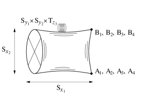
Figure 4: Visualisation of the 6d internal space after orbifolding. The two larger extra dimensions $S_{x_{1}}$ and $S_{x_{2}}$ parameterize a ‘half-pillow’ with crosscap identification on the left. Away from the two conical singularities on the right, every point of this 2d space supports 4 smaller extra dimensions with $T^{4}$ geometry.

5.1.1 Gauge embedding: a toy model

We now explicitly discuss the gauge embedding of the actions of $g$ and $g^{\prime}$. We begin with a simple example and continue, in the next subsection, with the much wider class of models with quantized Wilson lines including, in particular, an SO(10) GUT model broken non-locally to SU(4)$\times$SU(2)$\times$SU(2).

The most general gauge embedding of the action of $g^{\prime}$ and $g$ can be characterized by shift vectors

$$V^{\prime}=\frac{1}{2}\left(1^{n},\,0^{16-n}\right),\,\,\,\,V=\frac{1}{2}\left(0^{p},1^{m},\,0^{16-m-p}\right)\,$$ (46)

with $p<n<p+m$. The familiar requirements of modular invariance (for a recent collection of the relevant formulae see, e.g., [20]) impose $n=2\,{\rm mod}\,4$, $m=2\,{\rm mod}\,4$, and $p$ odd. The gauge symmetry breaking by $Z^{\prime}_{2}$ (at the high scale) is

$$SO(32)\begin{tabular}[]{c}local\\[-4.30554pt] $\longrightarrow$\end{tabular}SO(2n)\times SO(32-2n),$$ (47)

where $n=2,\,6,\,10,\,14$ are possible. The breaking by $Z_{2}$ (at the GUT scale) is

$$SO(2n)\begin{tabular}[]{c}non local\\[-4.30554pt] $\longrightarrow$\end{tabular}SO(2p)\times SO(2n-2p),$$ (50)

$$SO(32-2n)\begin{tabular}[]{c}non local\\[-4.30554pt] $\longrightarrow$\end{tabular}SO(2m+2p-2n)\times SO(32-2m-2p).$$ (53)

Within this toy model we can identify, for example, ‘$\mathcal{G}_{GUT}$’ $\equiv\,\,$SO$(2n)$ and ‘$\mathcal{G}_{SM}$’$\equiv\,\,$SO$(2p)\times$SO$(2n-2p)$. Clearly, one is severely limited by the fact that the GUT group can only be SO(12), SO(20) or SO(28).

5.1.2 A Pati-Salam model with two Wilson lines

The situation can be greatly improved by adding two Wilson lines to the system. In the next example, the $Z^{\prime}_{2}$ projection in the presence of Wilson lines breaks, at the high scale, SO(32) to SO(10)$\times\mathcal{G}$. We can now identify the GUT group with SO(10) and realize its further breaking to the Pati-Salam group SO(6)$\times$SO(4)$\,\equiv\,$SU(4)$\times$SU(2)$\times$SU(2) by the free action of $g^{\prime}$. Explicitly, we take

$$V^{\prime}=\frac{1}{2}\left(1^{10},0^{6}\right),\,\,\,\,V=\frac{1}{2}\left(0^{3},1^{2},0^{4},1^{4},0^{3}\right).$$ (54)

Note that these vectors are just a specific case of Eq. (46), where $n=10$, $m=6$, $p=7$ and Cartan generators have been reshuffled to bring $V$ to a form which will be more convenient later on. We also introduce the Wilson lines

$$A_{1}=\frac{1}{2}\left(0^{6},1^{8},0^{2}\right),\,\,\,\,A_{2}=\frac{1}{2}\left(0^{5},1,0^{3},1^{2},0^{4},1\right)$$ (55)

in $y_{1}$ and $y_{2}$ direction. Since the corresponding radii $R_{4}$ and $R_{5}$ are very short, the breaking introduced by these two Wilson lines is a high-scale breaking, realized everywhere in the 6d bulk spanned by the large radii $R_{1}$ and $R_{2}$ and the 4d Minkowski space. It is easy to see that the combined high-scale gauge symmetry breaking due to $V^{\prime}$, $A_{1}$ and $A_{2}$ is

$${\rm SO}(32) V^{\prime} \longrightarrow {\rm SO}(20)\times{\rm SO}(12)\begin{tabular}[]{c}$A_{1}$\\[-4.30554pt] $\longrightarrow$\end{tabular}{\rm SO}(12)\times{\rm SO}(8)\times{\rm SO}(8)\times{\rm SO}(4)$$

(60)

$$A_{2}$$

(63)

Identifying the GUT group with SO(10), the further breaking by $g$ (characterized by $V$) can be recognized as the desired non-local GUT breaking SO(10)$\,\rightarrow\,$SO(6)$\times$SO(4). At this point, we have to assume that a further breaking to the SM gauge group can be realized either field-theoretically (at least the doublet-triplet splitting problem is now solved) or in a better string model. We leave the search for such a more complete model for the future.

The choice of compactification radii shown in Figs. 3 and 4 and discussed in Sect. 3.3.1 ensures that the GUT symmetry breaking has the correct scale, couplings unify quantitatively in the perturbative domain of 6d field-theory, and that the perturbative calculation of the string spectrum can be trusted qualitatively. Furthermore, we assume bulk dominance (which should, according to Sect. 4, be marginally valid) and recall that we have ${\cal N}=4$ SUSY away from the fixed points. Under these two premisses, the SUSY-protected relations between $M_{P}$, $\alpha_{GUT}$, $g_{H}$ and ${\alpha^{\prime}}_{H}$ can be trusted quantitatively even though string-theoretic perturbativity at the high scale is, in general, lost.

5.2 Orbifold GUTs in 5 dimensions

This section is devoted to the implications of our general string-theoretic perturbativity analysis (and in particular the results of Sects. 3.3 and 4.2) for specific 5d unified models with brane localized GUT breaking (orbifold GUTs).

The simplest realistic orbifold GUTs have SU(5) symmetry in 5d, broken to the standard model group by appropriate $Z_{2}$ boundary conditions at one of the two boundaries (SM brane) [15, 16, 17]. In a minimalist setting, the two Higgs doublet superfields are introduced at this SM brane [17]. (At our level of precision, the bulk or brane nature of SM matter is irrelevant because it comes in full SU(5) multiplets.) In the setting with brane-localized Higgs doublets, the relative running of the differences of inverse gauge couplings (differential running) above $M_{c}$ is very close to the 4d MSSM: The relevant $\beta$ function coefficients are $(8/5,-2,-5)$ [17], which have to be compared with the MSSM values $(33/5,1,-3)$. To quantify the similarity of these two sets of coefficients, consider ratios of the differences $\Delta\alpha_{ij}=\alpha_{i}^{-1}-\alpha_{j}^{-1}$ created by the running ($i,j$ refer to the three SM gauge group factors), for example

$$\left(\frac{\Delta\alpha_{12}}{\Delta\alpha_{23}}\right)_{\mbox{MSSM}}=1.4\qquad\mbox{and}\qquad\left(\frac{\Delta\alpha_{12}}{\Delta\alpha_{23}}\right)_{\mbox{minimal orbif. GUT above $M_{c}$}}=1.2\,.$$ (64)

The similarity of these two ratios implies that unification will not be drastically affected even if part of the usual MSSM running is replaced by the modified running above $M_{c}$. The precision loss in the unification of the $\alpha_{i}^{-1}$ can be quantified as

$$\Delta\alpha_{\rm err}\simeq\frac{\ln(M_{GUT}/M_{c})}{\ln(M_{GUT}/m_{Z})}\cdot\frac{|1.2-1.4|}{1.4}\cdot 30\,,$$ (65)

based on the total change of the difference of, e.g., the first two inverse couplings in conventional MSSM unification, $\Delta\alpha_{12}(m_{Z})\simeq 30$.

However, even though the modified running does not significantly affect unification precision, it does change the final unification scale because the ‘speed’ of the modified running is reduced. Estimating the reduction factor as $(8/5\!+\!2)/(33/5\!-\!1)\simeq(-\!2\!+\!5)/(1\!+\!3)\simeq 0.7$, this raised final unification scale (which we identify with the UV scale $M$ of the relevant model) is determined by

$$\ln(M_{GUT}/m_{Z})\simeq\ln(M_{c}/m_{Z})+0.7\,\ln(M/M_{c})\,.$$ (66)

Now recall that in orbifold GUTs as well as in corresponding string models with strong coupling at $M$, a limit on the precision of gauge unification is set by the ratio $M/M_{c}$. If, on the one hand, $M_{c}$ is large (near $M_{GUT}$), Eq. (66) fixes the ultimate unification scale $M$ dangerously close to $M_{c}$. If, on the other hand, $M_{c}$ is small, Eq. (43) suggests that the UV scale $M$ (and thus $M/M_{c}$) is low because of the presence of light non-perturbative states. The optimal value is $M_{c}\simeq 2.6\times 10^{15}$ GeV, with $M/M_{c}\simeq 20$. Although not comfortably large, this value may still be consistent with the basic orbifold GUT idea of gauge unification based on bulk dominance.

We expect the following features arising in the above specific model to be generic: If the differential running above $M_{c}$ is similar to the MSSM running but ‘slower’, then $M>M_{GUT}>M_{c}$ and a certain validity range of 5d field theory (ensuring precision gauge coupling unification even in the case of a non-perturbative stringy UV completion at $M$) can be realized. The situation becomes better the slower the differential running above $M_{c}$ is. Ideally, one would want a model where, in spite of hard (from the field-theoretic perspective) GUT breaking at the boundary, no differential running above $M_{c}$ occurs. This would clearly require a very special bulk and brane field content.

In this paper, we have restricted ourselves to simple leading-log running, ignoring all other loop corrections. From this perspective, MSSM unification is perfect within the expected accuracy and the problem is merely to achieve consistency with string theory and the scale of gravity. A more careful analysis, including loop corrections at the weak/SUSY-breaking scale and 2-loop running, reveals that the $\alpha_{3}$ value predicted by grand unification is somewhat high (see [57] and refs. therein). In our opinion, this is not particularly serious in view of the significant high-scale uncertainties present, in particular, in string-based orbifold GUT models (recall the brane-localized non-universal gauge-kinetic terms). However, taking the discrepancy seriously, it was suggested early on that one can use the deviation of the differential running above $M_{c}$ from the MSSM running to account more accurately for the measured value of the strong coupling [22]. Without going into detail, we emphasize that the above string-theory-based restrictions on the size of the ratio $M/M_{c}$ apply and it may be necessary to reconsider such orbifold GUT models (with ‘improved’ unification) in this context.

We discussed 5d orbifold GUTs mainly using the perturbativity analysis of the SO(32) heterotic string. The E${}_{8}\times$E₈ case is also very relevant even though, as explained in Sect. 3.3.3, this scenario appears to be more constrained. A recent search for phenomenologically appealing string-theoretic orbifold GUT models of this type appeared in [19], where the unification scale problem was also discussed. The authors conclude that one is driven into the $M$ theory regime with the scales $\rho$ and $R_{l}$ very close (although the problem of small $R_{s}$ is not analysed). This is consistent with our findings, which we interpret more strongly as implying a serious problem for precision gauge coupling unification (insufficient volume suppression of non-perturbative brane effects).

We finally note that, in our understanding, the discussion of local breaking in this subsection is close in spirit to the very recent analysis of [10]. There, a mildly increased radius is used to bring the unification scale closer to the string scale. We believe that the underlying effect is related to the slower differential running above $M_{c}$ used in this subsection and discussed earlier in the context of orbifold GUTs.

6 Conclusions

We have discussed mass scales in heterotic string model building, attempting to use the compactification radii to explain the well-known discrepancy between the SUSY unification scale $M_{GUT}$ and the string scale $M_{string}$. Our starting point was the careful definition of a proper string coupling constant $g$ such that $g\!=\!1$ characterizes quantitatively the boundary of the perturbative regime of the heterotic string. We found surprisingly good agreement between a duality based and an effective field theory based definition of this string coupling.

Having rederived, with the above perturbativity definition, the well-known problems of isotropic compactifications, we focussed our attention on highly anisotropic orbifold geometries. Taking one of the compact radii larger than the other four, it is easy to move the corresponding compactification scale $M_{c}$ to the GUT scale without leaving the perturbative regime of string theory. However, it is unfortunately impossible to identify $M_{c}$ with the GUT breaking scale. The basic reason is that the compact geometry is that of an interval and that the GUT group is, in general, broken at one or both of its boundaries. The logarithmic running of gauge coupling differences then does not stop at $M_{c}$ but continues up to the string scale.

Nevertheless, this effective 5d scenario is interesting since the modified differential running between $M_{c}$ and the string scale may be used to realize a precise gauge coupling unification in spite of the fact that the running does not stop at $M_{GUT}$. In fact, lowering the smaller radii to below the string length and/or entering the string-theoretic strong coupling regime, it is even possible to take $M_{c}$ significantly below $M_{GUT}$. For example, we find it possible to have $M_{c}\simeq 2.6\times 10^{15}$ GeV while losing perturbative control only at a scale $M\sim 20M_{c}$. In this situation, the bulk suppression factor $1/20$ ensures (moderately) precise unification in spite of non-perturbative brane-localized effects at the scale $M$. Furthermore, the somewhat slower differential running above $M_{c}$ of the simplest orbifold GUTs improves the unification precision at the slightly high scale $M>M_{GUT}$.

An obvious disadvantage of the above and other related 5d scenarios is the model dependence introduced by the modified differential running above $M_{c}$. By contrast, in the case of two larger radii, it is possible to construct models where precise unification occurs just on the basis of the MSSM running between the electroweak scale and $M_{GUT}$.

The key is the observation that, even in the case of simple toroidal orbifolds, the geometry of the two larger extra dimensions of these 6d models can be sufficiently complicated to allow for a non-local GUT breaking (with the scale set by $M_{c}\simeq M_{GUT}$) together with an appropriate reduction of SUSY to ${\cal N}\!=\!1$. One has to pay the price of entering the non-perturbative regime of the underlying string theory sufficiently deeply so that one has to expect a breakdown of the 6d field theory very close to $M_{c}$. However, since the GUT breaking is non-local, the resulting non-perturbative contributions to gauge coupling differences are exponentially suppressed and a small hierarchy between $M_{c}$ and the strong coupling scale $M$ may be sufficient.

The technical tool used in the construction of the above models with two large radii and non-local breaking is the freely acting orbifold. The gauge symmetry is broken by non-local discrete Wilson lines, which can be viewed as an extension of the widely used method of discrete Wilson line breaking. To ensure that such Wilson lines introduce a non-local breaking (i.e., there are no fixed points with reduced gauge symmetry) it is necessary, starting from a torus with Wilson lines, to mod out rototranslations rather than simple rotations. We provide an explicit example where the original SO(32) gauge symmetry is broken near the string scale to a 6d SO(10) and then, by a non-local breaking at the GUT scale, to an SU(4)$\times$SU(2)$\times$SU(2) model in 4d.

In analysing how small the smaller of the orbifold radii can be made and at which energy scale string-theoretic perturbativity is lost, we had to rely heavily on $S$ and $T$ dualities. In particular, the above statements about the perturbativity loss in 5d or 6d field theory were based on going, via a network of dualities, to a weakly coupled description and identifying the lowest-lying (and thus most dangerous) massive string state. Our calculations were conservative in that we used toroidal compactifications and $T$ dualities in their basic form. However, we know that in the presence of Wilson lines (which are in any case necessary in realistic model building) $T$ duality constraints on the smallness of the small radii will be relaxed. Thus, we are confident that a large class of interesting models with the above promising features with respect to gauge coupling unification exist.

The $T$ dualities mentioned above and used extensively in our analysis of the type I dual of the SO(32) heterotic string are not available for the $M$ theory dual of the E${}_{8}\times$E₈ heterotic theory. Thus, our ability to analyse this case is significantly weaker (except for the special case with Wilson line breaking to SO(16)$\times$SO(16) which is dual to the SO(32) theory). Using conservative estimates on the minimal allowed size of the small compact dimensions, we find that both in the effective 5d and 6d case generic E${}_{8}\times$E₈ string theory completions are more constrained than the corresponding SO(32) models.

We believe to have shown that the GUT scale/string scale problem points to string compactifications where one or two of the compact radii are exceptionally large. The related phenomenological requirements, which have to a certain extent been explored in the field theory context, leave a wide field of possible activities on the side of string model building. We are particularly intrigued by the unexplored class of orbifold models where non-local discrete Wilson lines break the GUT group at the compactification scale.

Acknowledgements: We would like to thank Ignatios Antoniadis, Wilfried Buchmüller, Jan Louis, Stefan Groot Nibbelink, Marco Serone, Stephan Stieberger, Stuart Raby, Michael Ratz and Rodolfo Russo for useful comments and discussions.

References

- [1] D. J. Gross, J. A. Harvey, E. J. Martinec and R. Rohm, “Heterotic String Theory”, Nucl. Phys. B 256 (1985) 253 and 267 (1986) 75.
- [2] P. Candelas, G. T. Horowitz, A. Strominger and E. Witten, “Vacuum Configurations For Superstrings,” Nucl. Phys. B 258 (1985) 46.
- [3] L. J. Dixon, J. A. Harvey, C. Vafa and E. Witten, “Strings On Orbifolds”, Nucl. Phys. B 261 (1985) 678 and 274 (1986) 285.
- [4] V. S. Kaplunovsky, “Mass Scales Of The String Unification,” Phys. Rev. Lett. 55 (1985) 1036.
-
[5]
L. J. Dixon, V. Kaplunovsky and J. Louis, “Moduli Dependence Of String Loop
Corrections To Gauge Coupling Constants,” Nucl. Phys. B 355 (1991)
649;
I. Antoniadis, K. S. Narain and T. R. Taylor, “Higher genus string corrections to gauge couplings,” Phys. Lett. B 267 (1991) 37. -
[6]
L. E. Ibanez, D. Lüst and G. G. Ross,
“Gauge coupling running in minimal SU(3) x SU(2) x U(1) superstring
unification,”
Phys. Lett. B 272 (1991) 251
[arXiv:hep-th/9109053];
P. Mayr, H. P. Nilles and S. Stieberger, “String unification and threshold corrections,” Phys. Lett. B 317, 53 (1993) [arXiv:hep-th/9307171];
H. P. Nilles and S. Stieberger, “String unification, universal one-loop corrections and strongly coupled heterotic string theory,” Nucl. Phys. B 499, 3 (1997) [arXiv:hep-th/9702110]; “How to Reach the Correct and in String Theory,” Phys. Lett. B 367, 126 (1996)[arXiv:hep-th/9510009]. -
[7]
M. K. Gaillard and R. l. Xiu,
“Analysis of running coupling constant unification in string theory,”
Phys. Lett. B 296 (1992) 71
[arXiv:hep-ph/9206206];
G. Lopes Cardoso, D. Lüst and T. Mohaupt, “Threshold corrections and symmetry enhancement in string compactifications,” Nucl. Phys. B 450 (1995) 115 [arXiv:hep-th/9412209];
D. Ghilencea and G. G. Ross, “String thresholds and renormalization group evolution,” Nucl. Phys. B 569 (2000) 391 [arXiv:hep-ph/9908369]; “Precision prediction of gauge couplings and the profile of a string theory,” Nucl. Phys. B 606 (2001) 101 [arXiv:hep-ph/0102306]. -
[8]
A. E. Faraggi,
“Gauge coupling unification in superstring derived standard - like models,”
Phys. Lett. B 302 (1993) 202
[arXiv:hep-ph/9301268];
K. R. Dienes and A. E. Faraggi, “Making ends meet: String unification and low-energy data,” Phys. Rev. Lett. 75 (1995) 2646 [arXiv:hep-th/9505018]; “Gauge coupling unification in realistic free fermionic string models,” Nucl. Phys. B 457 (1995) 409 [arXiv:hep-th/9505046]. -
[9]
K. R. Dienes, A. E. Faraggi and J. March-Russell,
“String Unification, Higher Level Gauge Symmetries, and Exotic Hypercharge
Normalizations,”
Nucl. Phys. B 467 (1996) 44
[arXiv:hep-th/9510223];
G. B. Cleaver, A. E. Faraggi and D. V. Nanopoulos, “String derived MSSM and M-theory unification,” Phys. Lett. B 455 (1999) 135 [arXiv:hep-ph/9811427]. - [10] G. G. Ross, “Wilson line breaking and gauge coupling unification,” arXiv:hep-ph/0411057.
- [11] E. Witten, “Strong Coupling Expansion Of Calabi-Yau Compactification,” Nucl. Phys. B 471 (1996) 135 [arXiv:hep-th/9602070].
- [12] T. Banks and M. Dine, “Couplings and Scales in Strongly Coupled Heterotic String Theory,” Nucl. Phys. B 479 (1996) 173 [arXiv:hep-th/9605136].
- [13] E. Caceres, V. S. Kaplunovsky and I. M. Mandelberg, “Large-volume string compactifications, revisited,” Nucl. Phys. B 493 (1997) 73 [arXiv:hep-th/9606036].
-
[14]
J. R. Ellis, S. Kelley and D. V. Nanopoulos, “Precision Lep Data,
Supersymmetric Guts And String Unification,” Phys. Lett. B 249,
441 (1990);
U. Amaldi, W. de Boer and H. Fürstenau, “Comparison of grand unified theories with electroweak and strong coupling constants measured at LEP,” Phys. Lett. B 260, 447 (1991);
P. Langacker and M. X. Luo, “Implications of precision electroweak experiments for , , and grand unification,” Phys. Rev. D 44, 817 (1991). -
[15]
Y. Kawamura, “Triplet-doublet splitting, proton stability and extra
dimension,” Prog. Theor. Phys. 105 (2001) 999
[arXiv:hep-ph/0012125];
G. Altarelli and F. Feruglio, “SU(5) grand unification in extra dimensions and proton decay,” Phys. Lett. B 511 (2001) 257 [arXiv:hep-ph/0102301]. - [16] L. J. Hall and Y. Nomura, “Gauge unification in higher dimensions,” Phys. Rev. D 64, 055003 (2001) [arXiv:hep-ph/0103125].
- [17] A. Hebecker and J. March-Russell, “A minimal S(1)/(Z(2) x Z’(2)) orbifold GUT,” Nucl. Phys. B 613 (2001) 3 [arXiv:hep-ph/0106166].
-
[18]
T. Asaka, W. Buchmüller and L. Covi, “Gauge unification in six dimensions,”
Phys. Lett. B 523 (2001) 199 [arXiv:hep-ph/0108021];
L. J. Hall, Y. Nomura, T. Okui and D. R. Smith, “SO(10) unified theories in six dimensions,” Phys. Rev. D 65 (2002) 035008 [arXiv:hep-ph/0108071]. - [19] T. Kobayashi, S. Raby and R. J. Zhang, “Constructing 5d orbifold grand unified theories from heterotic strings,” arXiv:hep-ph/0403065.
- [20] S. Förste, H. P. Nilles, P. K. S. Vaudrevange and A. Wingerter, “Heterotic brane world,” arXiv:hep-th/0406208.
- [21] T. Kobayashi, S. Raby and R. J. Zhang, “Searching for realistic 4d string models with a Pati-Salam symmetry: Orbifold grand unified theories from heterotic string compactification on a Z(6) orbifold,” arXiv:hep-ph/0409098.
- [22] L. J. Hall and Y. Nomura, “Gauge coupling unification from unified theories in higher dimensions,” Phys. Rev. D 65 (2002) 125012 [arXiv:hep-ph/0111068].
-
[23]
C. Vafa and E. Witten, “Dual string pairs with N = 1 and N = 2
supersymmetry in four dimensions,” Nucl. Phys. Proc. Suppl. 46
(1996) 225 [arXiv:hep-th/9507050];
E. Kiritsis and C. Kounnas, “Perturbative and non-perturbative partial supersymmetry breaking: N = 4 N = 2 N = 1,” Nucl. Phys. B 503 (1997) 117 [arXiv:hep-th/9703059]. - [24] A. Hebecker, “Grand unification in the projective plane,” JHEP 0401, 047 (2004) [arXiv:hep-ph/0309313].
-
[25]
Y. Nomura, D. R. Smith and N. Weiner, “GUT breaking on the brane,”
Nucl. Phys. B 613 (2001) 147
[arXiv:hep-ph/0104041];
R. Contino, L. Pilo, R. Rattazzi and E. Trincherini, “Running and matching from 5 to 4 dimensions,” Nucl. Phys. B 622 (2002) 227 [arXiv:hep-ph/0108102]. - [26] I. Antoniadis and B. Pioline, “Low-scale closed strings and their duals,” Nucl. Phys. B 550 (1999) 41 [arXiv:hep-th/9902055].
- [27] P. H. Ginsparg, “Comment On Toroidal Compactification Of Heterotic Superstrings,” Phys. Rev. D 35 (1987) 648.
- [28] K. S. Choi, S. G. Nibbelink and M. Trapletti, “Heterotic SO(32) model building in four dimensions,” arXiv:hep-th/0410232.
- [29] J. Polchinski, “String theory. Vol. 2: Superstring theory and beyond”, Cambridge University Press, 1998.
- [30] P. Di Vecchia, L. Magnea, A. Lerda, R. Russo and R. Marotta, “String techniques for the calculation of renormalization constants in field theory,” Nucl. Phys. B 469 (1996) 235 [arXiv:hep-th/9601143].
- [31] J. Polchinski and E. Witten, “Evidence for Heterotic - Type I String Duality,” Nucl. Phys. B 460 (1996) 525 [arXiv:hep-th/9510169].
- [32] N. Sakai and M. Abe, “Coupling Constant Relations And Effective Lagrangian In The Type I Superstring,” Prog. Theor. Phys. 80 (1988) 162.
- [33] A. A. Tseytlin, “On SO(32) heterotic - type I superstring duality in ten dimensions,” Phys. Lett. B 367 (1996) 84 [arXiv:hep-th/9510173].
- [34] P. Horava and E. Witten, “Heterotic and type I string dynamics from eleven dimensions,” Nucl. Phys. B 460 (1996) 506 [arXiv:hep-th/9510209]; “Eleven-Dimensional Supergravity on a Manifold with Boundary,” Nucl. Phys. B 475, 94 (1996) [arXiv:hep-th/9603142],
-
[35]
J. O. Conrad,
“Brane tensions and coupling constants from within M-theory,”
Phys. Lett. B 421 (1998) 119
[arXiv:hep-th/9708031];
T. Harmark, “Coupling constants and brane tensions from anomaly cancellation in M-theory,” Phys. Lett. B 431 (1998) 295 [arXiv:hep-th/9802190]. - [36] Z. Chacko, M. A. Luty and E. Ponton, “Massive higher-dimensional gauge fields as messengers of supersymmetry breaking,” JHEP 0007 (2000) 036 [arXiv:hep-ph/9909248].
- [37] T. van Ritbergen, A. N. Schellekens and J. A. M. Vermaseren, “Group theory factors for Feynman diagrams,” Int. J. Mod. Phys. A 14 (1999) 41 [arXiv:hep-ph/9802376].
- [38] I. Antoniadis and S. Dimopoulos, “Splitting supersymmetry in string theory,” arXiv:hep-th/0411032.
-
[39]
K. Kikkawa and M. Yamasaki,
“Casimir Effects In Superstring Theories,”
Phys. Lett. B 149, 357 (1984).
T. H. Buscher, “Path Integral Derivation Of Quantum Duality In Nonlinear Sigma Models,” Phys. Lett. B 201 (1988) 466. -
[40]
N. Seiberg, “Five dimensional SUSY field theories, non-trivial fixed points
and string dynamics,” Phys. Lett. B 388 (1996) 753
[arXiv:hep-th/9608111], “Non-trivial fixed points of the renormalization
group in six dimensions,” Phys. Lett. B 390 (1997) 169
[arXiv:hep-th/9609161];
K. R. Dienes, E. Dudas and T. Gherghetta, “GUT precursors and non-trivial fixed points in higher-dimensional gauge theories,” Phys. Rev. Lett. 91 (2003) 061601 [arXiv:hep-th/0210294]. -
[41]
J. Dai, R. G. Leigh and J. Polchinski, “New Connections Between String
Theories,” Mod. Phys. Lett. A 4 (1989) 2073;
J. Polchinski, “Lectures on D-branes,” arXiv:hep-th/9611050. - [42] K. S. Narain, M. H. Sarmadi and E. Witten, “A Note On Toroidal Compactification Of Heterotic String Theory,” Nucl. Phys. B 279 (1987) 369.
- [43] S. F. Hassan, “T duality and nonlocal realizations of supersymmetry in string theory,” [arXiv:hep-th/9511056]; “T Duality and nonlocal supersymmetries,” Nucl. Phys. B 460, 362 (1996) [arXiv:hep-th/9504148]; “O(d,d:R) deformations of complex structures and extended world sheet Nucl. Phys. B 454, 86 (1995) [arXiv:hep-th/9408060].
- [44] J. Scherk and J. H. Schwarz, “How To Get Masses From Extra Dimensions,” Nucl. Phys. B 153 (1979) 61.
- [45] Y. Hosotani, “Dynamical Mass Generation By Compact Extra Dimensions,” Phys. Lett. B 126 (1983) 309; “Dynamics Of Nonintegrable Phases And Gauge Symmetry Breaking,” Annals Phys. 190 (1989) 233.
- [46] E. Witten, “Symmetry Breaking Patterns In Superstring Models,” Nucl. Phys. B 258 (1985) 75.
-
[47]
T. Friedmann and E. Witten, “Unification scale, proton decay, and
manifolds of G(2) holonomy,” Adv. Theor. Math. Phys. 7 (2003)
577 [arXiv:hep-th/0211269];
R. Donagi, Y. H. He, B. A. Ovrut and R. Reinbacher, “The spectra of heterotic standard model vacua,” arXiv:hep-th/0411156. -
[48]
R. Rohm,
“Spontaneous Supersymmetry Breaking In Supersymmetric String Theories,”
Nucl. Phys. B 237, 553 (1984);
C. Kounnas and M. Porrati, “Spontaneous Supersymmetry Breaking In String Theory,” Nucl. Phys. B 310, 355 (1988);
S. Ferrara, C. Kounnas, M. Porrati and F. Zwirner, “Superstrings With Spontaneously Broken Supersymmetry And Their Effective Theories,” Nucl. Phys. B 318, 75 (1989). - [49] C. Kounnas and B. Rostand, “Coordinate Dependent Compactifications And Discrete Symmetries,” Nucl. Phys. B 341 (1990) 641.
-
[50]
E. Kiritsis and C. Kounnas,
“Perturbative and non-perturbative partial supersymmetry breaking: N = 4
N = 2 N = 1,”
Nucl. Phys. B 503, 117 (1997)
[arXiv:hep-th/9703059];
C. A. Scrucca and M. Serone, “A novel class of string models with Scherk-Schwarz supersymmetry breaking,” JHEP 0110, 017 (2001) [arXiv:hep-th/0107159]. -
[51]
I. Antoniadis, E. Dudas and A. Sagnotti,
“Brane supersymmetry breaking,”
Phys. Lett. B 464, 38 (1999)
[arXiv:hep-th/9908023];
I. Antoniadis, G. D’Appollonio, E. Dudas and A. Sagnotti, “Open descendants of Z(2) x Z(2) freely-acting orbifolds,” Nucl. Phys. B 565, 123 (2000) [arXiv:hep-th/9907184];
A. L. Cotrone, “A Z(2) x Z(2) orientifold with spontaneously broken supersymmetry,” Mod. Phys. Lett. A 14, 2487 (1999) [arXiv:hep-th/9909116];
C. A. Scrucca, M. Serone and M. Trapletti, “Open string models with Scherk-Schwarz SUSY breaking and localized anomalies,” Nucl. Phys. B 635, 33 (2002) [arXiv:hep-th/0203190]. - [52] L. J. Hall, H. Murayama and Y. Nomura, “Wilson lines and symmetry breaking on orbifolds,” Nucl. Phys. B 645 (2002) 85 [arXiv:hep-th/0107245].
-
[53]
L. E. Ibanez, H. P. Nilles and F. Quevedo,
“Reducing The Rank Of The Gauge Group In Orbifold Compactifications Of The
Heterotic String,”
Phys. Lett. B 192 (1987) 332;
L. E. Ibanez, J. Mas, H. P. Nilles and F. Quevedo, “Heterotic Strings In Symmetric And Asymmetric Orbifold Backgrounds,” Nucl. Phys. B 301 (1988) 157. -
[54]
T. Mohaupt,