From Physics to Number theory via Noncommutative Geometry, II

Chapter 2 Renormalization, the Riemann–Hilbert correspondence, and motivic Galois theory

Contents

1. 2 Renormalization, the Riemann–Hilbert correspondence, and motivic Galois theory
   1. 2.1 Introduction
   2. 2.2 Renormalization in Quantum Field Theory
      1. 2.2.1 Basic formulas of QFT
      2. 2.2.2 Feynman diagrams
      3. 2.2.3 Divergences and subdivergences
   3. 2.3 Affine group schemes
      1. 2.3.1 Tannakian categories
      2. 2.3.2 The Lie algebra and the Milnor-Moore theorem
   4. 2.4 The Hopf algebra of Feynman graphs and diffeographisms
   5. 2.5 The Lie algebra of graphs
   6. 2.6 Birkhoff decomposition and renormalization
   7. 2.7 Unit of Mass
   8. 2.8 Expansional
   9. 2.9 Renormalization group
   10. 2.10 Diffeographisms and diffeomorphisms
   11. 2.11 Riemann–Hilbert problem
       1. 2.11.1 Regular-singular case
       2. 2.11.2 Local Riemann–Hilbert problem and Birkhoff decomposition
       3. 2.11.3 Geometric formulation
       4. 2.11.4 Irregular case
   12. 2.12 Local equivalence of meromorphic connections
   13. 2.13 Classification of equisingular flat connections
   14. 2.14 The universal singular frame
   15. 2.15 Mixed Tate motives
       1. 2.15.1 Motives and noncommutative geometry: analogies
       2. 2.15.2 Motivic fundamental groupoid
       3. 2.15.3 Expansional and multiple polylogarithms
   16. 2.16 The “cosmic Galois group” of renormalization as a motivic Galois group
   17. 2.17 The wild fundamental group
   18. 2.18 Questions and directions
       1. 2.18.1 Renormalization of geometries
       2. 2.18.2 Nonperturbative effects
       3. 2.18.3 The field of physical constants
       4. 2.18.4 Birkhoff decomposition and integrable systems
   19. 2.19 Further developments

2.1 Introduction

We give here a comprehensive treatment of the mathematical theory of perturbative renormalization (in the minimal subtraction scheme with dimensional regularization), in the framework of the Riemann–Hilbert correspondence and motivic Galois theory. We give a detailed overview of the work of Connes–Kreimer [31], [32]. We also cover some background material on affine group schemes, Tannakian categories, the Riemann–Hilbert problem in the regular singular and irregular case, and a brief introduction to motives and motivic Galois theory. We then give a complete account of our results on renormalization and motivic Galois theory announced in [35].

Our main goal is to show how the divergences of quantum field theory, which may at first appear as the undesired effect of a mathematically ill-formulated theory, in fact reveal the presence of a very rich deeper mathematical structure, which manifests itself through the action of a hidden “cosmic Galois group”, which is of an arithmetic nature, related to motivic Galois theory.

Historically, perturbative renormalization has always appeared as one of the most elaborate recipes created by modern physics, capable of producing numerical quantities of great physical relevance out of a priori meaningless mathematical expressions. In this respect, it is fascinating for mathematicians and physicists alike. The depth of its origin in quantum field theory and the precision with which it is confirmed by experiments undoubtedly make it into one of the jewels of modern theoretical physics.

For a mathematician in quest of “meaning” rather than heavy formalism, the attempts to cast the perturbative renormalization technique in a conceptual framework were so far falling short of accounting for the main computational aspects, used for instance in QED. These have to do with the subtleties involved in the subtraction of infinities in the evaluation of Feynman graphs and do not fall under the range of “asymptotically free theories” for which constructive quantum field theory can provide a mathematically satisfactory formulation.

The situation recently changed through the work of Connes–Kreimer ([29], [30], [31], [32]), where the conceptual meaning of the detailed computational devices used in perturbative renormalization is analysed. Their work shows that the recursive procedure used by physicists is in fact identical to a mathematical method of extraction of finite values known as the Birkhoff decomposition, applied to a loop $\gamma(z)$ with values in a complex pro-unipotent Lie group $G$.

This result, and the close relation between the Birkhoff factorization of loops and the Riemann–Hilbert problem, suggested the existence of a geometric interpretation of perturbative renormalization in terms of the Riemann–Hilbert correspondence. Our main result in this paper is to identify explicitly the Riemann–Hilbert correspondence underlying perturbative renormalization in the minimal subtraction scheme with dimensional regularization.

Performing the Birkhoff (or Wiener-Hopf) decomposition of a loop $\gamma(z)\in G$ consists of describing it as a product

$$\gamma\,(z)=\gamma_{-}(z)^{-1}\,\gamma_{+}(z)\qquad z\in C\,,$$ (2.1)

of boundary values of holomorphic maps (which we still denote by the same symbol)

$$\gamma_{\pm}:C_{\pm}\rightarrow G\,.$$ (2.2)

defined on the connected components $C_{\pm}$ of the complement of the curve $C$ in the Riemann sphere ${\mathbb{P}}^{1}({\mathbb{C}})$.

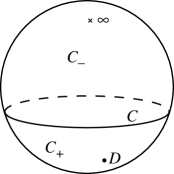
Figure 2.1: Birkhoff Decomposition

The geometric meaning of this decomposition, for instance when $G={\rm GL}_{n}({\mathbb{C}})$, comes directly from the theory of holomorphic bundles with structure group $G$ on the Riemann sphere ${\mathbb{P}}^{1}({\mathbb{C}})$. The loop $\gamma(z)$ describes the clutching data to construct the bundle from its local trivialization and the Birkhoff decomposition provides a global trivialization of this bundle. While in the case of ${\rm GL}_{n}({\mathbb{C}})$ the existence of a Birkhoff decomposition may be obstructed by the non-triviality of the bundle, in the case of a pro-unipotent complex Lie group $G$, as considered in the CK theory of renormalization, it is always possible to obtain a factorization (2.1).

In perturbative renormalization the points of ${\mathbb{P}}^{1}({\mathbb{C}})$ are “complex dimensions”, among which the dimension $D$ of the relevant space-time is a preferred point. The little devil that conspires to make things interesting makes it impossible to just evaluate the relevant physical observables at the point $D$, by letting them diverge precisely at that point. One can nevertheless encode all the evaluations at points $z\neq D$ in the form of a loop $\gamma(z)$ with values in the group $G$. The perturbative renormalization technique then acquires the following general meaning: while $\gamma(D)$ is meaningless, the physical quantities are in fact obtained by evaluating $\gamma_{+}(D)$, where $\gamma_{+}$ is the term that is holomorphic at $D$ for the Birkhoff decomposition relative to an infinitesimal circle with center $D$.

Thus, renormalization appears as a special case of a general principle of extraction of finite results from divergent expressions based on the Birkhoff decomposition.

The nature of the group $G$ involved in perturbative renormalization was clarified in several steps in the work of Connes–Kreimer (CK). The first was Kreimer’s discovery [79] of a Hopf algebra structure underlying the recursive formulae of [7], [71], [111]. The resulting Hopf algebra of rooted trees depends on the physical theory ${\mathcal{T}}$ through the use of suitably decorated trees. The next important ingredient was the similarity between the Hopf algebra of rooted trees of [79] and the Hopf algebra governing the symmetry of transverse geometry in codimension one of [39], which was observed already in [29]. The particular features of a given physical theory were then better encoded by a Hopf algebra defined in [31] directly in terms of Feynman graphs. This Hopf algebra of Feynman graphs depends on the theory ${\mathcal{T}}$ by construction. It determines $G$ as the associated affine group scheme, which is referred to as diffeographisms of the theory, $G={\rm Difg}({\mathcal{T}})$. Through the Milnor-Moore theorem [92], the Hopf algebra of Feynman graphs determines a Lie algebra, whose corresponding infinite dimensional pro-unipotent Lie group is given by the complex points $G({\mathbb{C}})$ of the affine group scheme of diffeographisms.

This group is related to the formal group of Taylor expansions of diffeomorphisms. It is this infinitesimal feature of the expansion that accounts for the “perturbative” aspects inherent to the computations of Quantum Field Theory. The next step in the CK theory of renormalization is the construction of an action of ${\rm Difg}({\mathcal{T}})$ on the coupling constants of the physical theory, which shows a close relation between ${\rm Difg}({\mathcal{T}})$ and the group of diffeomorphisms of the space of Lagrangians.

In particular, this allows one to lift the renormalization group to a one parameter subgroup of ${\rm Difg}$, defined intrinsically from the independence of the term $\gamma_{-}(z)$ in the Birkhoff decomposition from the choice of an additional mass scale $\mu$. It also shows that the polar expansions of the divergences are entirely determined by their residues (a strong form of the ’t Hooft relations), through the scattering formula of [32]

$$\gamma_{-}(z)=\lim_{t\to\infty}e^{-t\left(\frac{\beta}{z}+Z_{0}\right)}\,e^{tZ_{0}}\,.$$ (2.3)

After a brief review of perturbative renormalization in QFT (§2.2), we give in Sections 2.4, 2.5, 2.6, 2.10, and in part of Section 2.9, a detailed account of the main results mentioned above of the CK theory of perturbative renormalization and its formulation in terms of Birkhoff decomposition. This overview of the work of Connes–Kreimer is partly based on an English translation of [24] [25].

The starting point for our interpretation of renormalization as a Riemann–Hilbert correspondence is presented in Sections 2.8 and 2.9. It consists of rewriting the scattering formula (2.3) in terms of the time ordered exponential of physicists (also known as expansional in mathematical terminology), as

$$\gamma_{-}(z)={\bf{\rm T}e^{-\frac{1}{z}\,\int_{0}^{\infty}\,\theta_{-t}(\beta)\,dt}},$$ (2.4)

where $\theta_{t}$ is the one-parameter group of automorphisms implementing the grading by loop number on the Hopf algebra of Feynman graphs. We exploit the more suggestive form (2.4) to clarify the relation between the Birkhoff decomposition used in [31] and a form of the Riemann-Hilbert correspondence.

In general terms, as we recall briefly in Section 2.11, the Riemann–Hilbert correspondence is an equivalence between a class of singular differential systems and representation theoretic data. The classical example is that of regular singular differential systems and their monodromy representation.

In our case, the geometric problem underlying perturbative renormalization consists of the classification of “equisingular” $G$-valued flat connections on the total space $B$ of a principal $\mathbb{G}_{m}$-bundle over an infinitesimal punctured disk $\Delta^{*}$. An equisingular connection is a $\mathbb{G}_{m}$-invariant $G$-valued connection, singular on the fiber over zero, and satisfying the following property: the equivalence class of the singularity of the pullback of the connection by a section of the principal $\mathbb{G}_{m}$-bundle only depends on the value of the section at the origin.

The physical significance of this geometric setting is the following. The expression (2.4) in expansional form can be recognized as the solution of a differential system

$$\gamma^{-1}\,d\gamma=\omega.$$ (2.5)

This identifies a class of connections naturally associated to the differential of the regularized quantum field theory, viewed as a function of the complexified dimension. The base $\Delta^{*}$ is the space of complexified dimensions around the critical dimension $D$. The fibers of the principal $\mathbb{G}_{m}$-bundle $B$ describe the arbitrariness in the normalization of integration in complexified dimension $z\in\Delta^{*}$, in the Dim-Reg regularization procedure. The $\mathbb{G}_{m}$-action corresponds to the rescaling of the normalization factor of integration in complexified dimension $z$, which can be described in terms of the scaling $\hbar\,\,\partial/\partial\hbar$ on the expansion in powers of $\hbar$. The group defining $G$-valued connections is $G={\rm Difg}({\mathcal{T}})$. The physics input that the counterterms are independent of the additional choice of a unit of mass translates, in geometric terms, into the notion of equisingularity for the connections associated to the differential systems (2.5).

On the other side of our Riemann–Hilbert correspondence, the representation theoretic setting equivalent to the classification of equisingular flat connections is provided by finite dimensional linear representations of a universal group $U^{*}$, unambiguously defined independently of the physical theory. Our main result is the explicit description of $U^{*}$ as the semi-direct product by its grading of the graded pro-unipotent Lie group $U$ whose Lie algebra is the free graded Lie algebra

$$\mathcal{F}(1,2,3,\cdots)_{\bullet}$$

generated by elements $e_{-n}$ of degree $n$, $n>0$. As an affine group scheme, $U^{*}$ is identified uniquely via the formalism of Tannakian categories. Namely, equisingular flat connections on finite dimensional vector bundles can be can be organized into a Tannakian category with a natural fiber functor to the category of vector spaces. This category is equivalent to the category of finite dimensional representations of the affine group scheme $U^{*}$. These main results are presented in detail in Sections 2.12, 2.13, and 2.16.

This identifies a new level at which Hopf algebra structures enter the theory of perturbative renormalization, after Kreimer’s Hopf algebra of rooted trees and the CK Hopf algebra of Feynman graphs. Namely, the Hopf algebra associated to the affine group scheme $U^{*}$ is universal with respect to the set of physical theories. The “motivic Galois group” $U$ acts on the set of dimensionless coupling constants of physical theories, through the map $U^{*}\to{\rm Difg}^{*}$ to the group of diffeographisms of a given theory, which in turns maps to formal diffeomorphisms as shown in [32]. Here ${\rm Difg}^{*}$ is the semi-direct product of ${\rm Difg}$ by the action of the grading $\theta_{t}$, as in [32].

We then construct in Section 2.14 a specific universal singular frame on principal $U$-bundles over $B$. We show that, when using in this frame the dimensional regularization technique of QFT, all divergences disappear and one obtains a finite theory which only depends upon the choice of a local trivialization for the principal $\mathbb{G}_{m}$-bundle $B$ and produces the physical theory in the minimal subtraction scheme.

The coefficients of the universal singular frame, written out in the expansional form, are the same as those appearing in the local index formula of Connes–Moscovici [38]. This leads to the very interesting question of the explicit relation to noncommutative geometry and the local index formula.

In particular, the coefficients of the universal singular frame are rational numbers. This means that we can view equisingular flat connections on finite dimensional vector bundles as endowed with arithmetic structure. Thus, the Tannakian category of flat equisingular bundles can be defined over any field of characteristic zero. Its properties are very reminiscent of the formalism of mixed Tate motives (which we recall briefly in Section 2.15).

In fact, group schemes closely related to $U^{*}$ appear in motivic Galois theory. For instance, $U^{*}$ is abstractly (but non-canonically) isomorphic to the motivic Galois group $G_{{\mathcal{M}}_{T}}({\mathcal{O}})$ ([47], [66]) of the scheme $S_{4}={\rm Spec}({\mathcal{O}})$ of $4$-cyclotomic integers, ${\mathcal{O}}=\,{\mathbb{Z}}[i][\frac{1}{2}]$.

The existence of a universal pro-unipotent group $U$ underlying the theory of perturbative renormalization, canonically defined and independent of the physical theory, confirms a suggestion made by Cartier in [15], that in the Connes–Kreimer theory of perturbative renormalization one should find a hidden “cosmic Galois group” closely related in structure to the Grothendieck–Teichmüller group. The question of relations between the work of Connes–Kreimer, motivic Galois theory, and deformation quantization was further emphasized by Kontsevich in [76], as well as the conjecture of an action of a motivic Galois group on the coupling constants of physical theories. At the level of the Hopf algebra of rooted trees, relations between renormalization and motivic Galois theory were also investigated by Goncharov in [67].

Our result on the “cosmic motivic Galois group” $U$ also shows that the renormalization group appears as a canonical one parameter subgroup $\mathbb{G}_{a}\,\subset U$. Thus, this realizes the hope formulated in [24] of relating concretely the renormalization group to a Galois group.

As we discuss in Section 2.17, the group $U$ presents similarities with the exponential torus part of the wild fundamental group, in the sense of Differential Galois Theory (cf. [88], [102]). The latter is a modern form of the “theory of ambiguity” that Galois had in mind and takes a very concrete form in the work of Ramis [104]. The “wild fundamental group” is the natural object that replaces the usual fundamental group in extending the Riemann–Hilbert correspondence to the irregular case (cf. [88]). At the formal level, in addition to the monodromy representation (which is trivial in the case of the equisingular connections), it comprises the exponential torus, while in the non-formal case additional generators are present that account for the Stokes phenomena in the resummation of divergent series. The Stokes part of the wild fundamental group (cf. [88]) in fact appears when taking into account the presence of non-perturbative effects. We formulate some questions related to extending the CK theory of perturbative renormalization to the nonperturbative case.

We also bring further evidence for the interpretation of the renormalization group in terms of a theory of ambiguity. Indeed, one aspect of QFT that appears intriguing to the novice is the fact that many quantities called “constants”, such as the fine structure constant in QED, are only nominally constant, while in fact they depend on a scale parameter $\mu$. Such examples are abundant, as most of the relevant physical quantities, including the coupling “constants”, share this implicit dependence on the scale $\mu$. Thus, one is really dealing with functions $g(\mu)$ instead of scalars. This suggests the idea that a suitable “unramified” extension $K$ of the field ${\mathbb{C}}$ of complex numbers might play a role in QFT as a natural extension of the “field of constants” to a field containing functions whose basic behaviour is dictated by the renormalization group equations. The group of automorphisms of the resulting field, generated by $\mu\partial/\partial\mu$, is the group of ambiguity of the physical theory and it should appear as the Galois group of the unramified extension. Here the beta function of renormalization can be seen as logarithm of the monodromy in a regular-singular local Riemann–Hilbert problem associated to this scaling action as in [42]. The true constants are then the fixed points of this group, which form the field ${\mathbb{C}}$ of complex numbers, but a mathematically rigorous formulation of QFT may require extending the field of scalars first, instead of proving existence “over ${\mathbb{C}}$”.

This leads naturally to a different set of questions, related to the geometry of arithmetic varieties at the infinite primes, and a possible Galois interpretation of the connected component of the identity in the idèle class group in class field theory (cf. [23], [41]). This set of questions will be dealt with in [37].

Acknowledgements. We are very grateful to Jean–Pierre Ramis for many useful comments on an early draft of this paper, for the kind invitation to Toulouse, and for the many stimulating discussions we had there with him, Frédéric Fauvet, and Laurent Stolovitch. We thank Frédéric Menous and Giorgio Parisi for some useful correspondence. Many thanks go to Dirk Kreimer, whose joint work with AC on perturbative renormalization is a main topic of this Chapter.

2.2 Renormalization in Quantum Field Theory

The physical motivation behind the renormalization technique is quite clear and goes back to the concept of effective mass and to the work of Green in nineteenth century hydrodynamics [68]. To appreciate it, one should dive under water with a ping-pong ball and start applying Newton’s law,

$$F=m\,a$$ (2.6)

to compute the initial acceleration of the ball $B$ when we let it loose (at zero speed relative to the still water). If one naively applies (2.6), one finds an unrealistic initial acceleration of about $11.4\,g$. In fact, if one performs the experiment, one finds an initial acceleration of about $1.6\,g$. As explained by Green in [68], due to the interaction of $B$ with the surrounding field of water, the inertial mass $m$ involved in (2.6) is not the bare mass $m_{0}$ of $B$, but it is modified to

$$m=m_{0}+{\textstyle\frac{1}{2}}\,M$$ (2.7)

where $M$ is the mass of the water occupied by $B$. It follows for instance that the initial acceleration $a$ of $B$ is given, using the Archimedean law, by

$$-(M-m_{0})\,g=\left(m_{0}+{\textstyle\frac{1}{2}}\,M\right)a$$ (2.8)

and is always of magnitude less than $2g$.

The additional inertial mass $\delta\,m=m-m_{0}$ is due to the interaction of $B$ with the surrounding field of water and if this interaction could not be turned off (which is the case if we deal with an electron instead of a ping-pong ball) there would be no way to measure the bare mass $m_{0}$.

The analogy between hydrodynamics and electromagnetism led, through the work of Thomson, Lorentz, Kramers, etc. (cf. [49]), to the crucial distinction between the bare parameters, such as $m_{0}$, which enter the field theoretic equations, and the observed parameters, such as the inertial mass $m$.

Around 1947, motivated by the experimental findings of spectroscopy of the fine structure of spectra, physicists were able to exploit the above distinction between these two notions of mass (bare and observed), and similar distinctions for the charge and field strength, in order to eliminate the unwanted infinities which plagued the computations of QFT, due to the pointwise nature of the electron. We refer to [49] for an excellent historical account of that period.

2.2.1 Basic formulas of QFT

A quantum field theory in $D=4$ dimensions is given by a classical action functional

$$S\,(A)=\int{\mathcal{L}}\,(A)\,d^{4}x,$$ (2.9)

where $A$ is a classical field and the Lagrangian is of the form

$${\mathcal{L}}\,(A)=\frac{1}{2}(\partial A)^{2}-\frac{m^{2}}{2}\,A^{2}-{\mathcal{L}}_{\rm int}(A),$$ (2.10)

with $(\partial A)^{2}=(\partial_{0}A)^{2}-\sum_{\mu\neq 0}(\partial_{\mu}A)^{2}$. The term ${\mathcal{L}}_{\rm int}(A)$ is usually a polynomial in $A$.

The basic transition from “classical field theory” to “quantum field theory” replaces the classical notion of probabilities by probability amplitudes and asserts that the probability amplitude of a classical field configuration $A$ is given by the formula of Dirac and Feynman

$$e^{i\,\frac{S(A)}{\hbar}},$$ (2.11)

where $S(A)$ is the classical action (2.9) and $\hbar$ is the unit of action, so that $iS(A)/\hbar$ is a dimensionless quantity.

Thus, one can define the quantum expectation value of a classical observable (i.e. of a function ${\mathcal{O}}$ of the classical fields) by the expression

$$\langle{\mathcal{O}}\rangle=\,{\mathcal{N}}\,\int{\mathcal{O}}(A)\,e^{i\,\frac{S(A)}{\hbar}}\,D[A],\,$$ (2.12)

where ${\mathcal{N}}$ is a normalization factor. The (Feynman) integral has only formal meaning, but this suffices in the case where the space of classical fields $A$ is a linear space in order to define without difficulty the terms in the perturbative expansion, which make the renormalization problem manifest.

One way to describe the quantum fields $\phi(x)$ is by means of the time ordered Green’s functions

$$G_{N}(x_{1},\ldots,x_{N})=\langle\,0\,|T\,\phi(x_{1})\ldots\phi(x_{N})|\,0\,\rangle,$$ (2.13)

where the time ordering symbol $T$ means that the $\phi(x_{j})$’s are written in order of increasing time from right to left. If one could ignore the renormalization problem, the Green’s functions would then be computed as

$$G_{N}(x_{1},\ldots,x_{N})={\mathcal{N}}\int e^{i\,\frac{S(A)}{\hbar}}\ A(x_{1})\ldots A(x_{N})\,[dA],$$ (2.14)

where the factor ${\mathcal{N}}$ ensures the normalization of the vacuum state

$$\langle\,0\mid 0\,\rangle=1\,.$$ (2.15)

If one could ignore renormalization, the functional integral (2.14) would be easy to compute in perturbation theory, i.e. by treating the term ${\mathcal{L}}_{\rm int}$ in (2.10) as a perturbation of

$${\mathcal{L}}_{0}(A)=\frac{1}{2}(\partial A)^{2}-\frac{m^{2}}{2}\,A^{2}\,.$$ (2.16)

The action functional correspondingly splits as the sum of two terms

$$S(A)=S_{0}(A)+S_{\rm int}(A),$$ (2.17)

where the free action $S_{0}$ generates a Gaussian measure

$$\exp\,(i\,S_{0}(A))\,[dA]=d\mu,$$

where we have set $\hbar=1$.

The series expansion of the Green’s functions is then of the form

$$G_{N}(x_{1},\ldots,x_{N})=\left(\sum_{n=0}^{\infty}\,i^{n}/n!\int A(x_{1})\ldots A(x_{N})\,(S_{\rm int}(A))^{n}\,d\mu\right)$$

$$\quad\left(\sum_{n=0}^{\infty}\,i^{n}/n!\int S_{\rm int}(A)^{n}\,d\mu\right)^{-1}\,.$$

2.2.2 Feynman diagrams

The various terms

$$\int A(x_{1})\ldots A(x_{N})\,(S_{\rm int}(A))^{n}\,d\mu$$ (2.18)

of this expansion are integrals of polynomials under a Gaussian measure $d\mu$. When these are computed using integration by parts, the process generates a large number of terms $U(\Gamma)$. The combinatorial data labelling each of these terms are encoded in the Feynman graph $\Gamma$, which determines the terms that appear in the calculation of the corresponding numerical value $U(\Gamma)$, obtained as a multiple integral in a finite number of space-time variables. The $U(\Gamma)$ is called the unrenormalized value of the graph $\Gamma$.

One can simplify the combinatorics of the graphs involved in these calculations, by introducing a suitable generating function. The generating function for the Green’s functions is given by the Fourier transform

$$Z(J)={\mathcal{N}}\int\exp\left(i\frac{S(A)+\langle J,A\rangle}{\hbar}\right)\,[dA]$$ (2.19)

$$=\sum_{N=0}^{\infty}\frac{i^{N}}{N!}\int J(x_{1})\ldots J(x_{N})\,G_{N}(x_{1},..x_{N})\,dx_{1}..dx_{N},$$

where the source $J$ is an element of the dual of the linear space of classical fields $A$.

The zoology of the diagrams involved in the perturbative expansion is substantially simplified by first passing to the logarithm of $Z(J)$ which is the generating function for connected Green’s functions $G_{c}$,

$$iW(J)={\rm Log}(Z(J))=\,\sum_{N=0}^{\infty}\frac{i^{N}}{N!}\int J(x_{1})\ldots J(x_{N})G_{N,c}(x_{1},..x_{N})dx_{1}..dx_{N}.$$ (2.20)

At the formal combinatorial level, while the original sum (2.19) is on all graphs (including non-connected ones), taking the $\log$ in the expression (2.20) for $W(J)$ has the effect of dropping all disconnected graphs, while the normalization factor ${\mathcal{N}}$ in (2.19) eliminates all the “vacuum bubbles”, that is, all the graphs that do not have external legs. Moreover, the number $L$ of loops in a connected graph determines the power $\hbar^{L-1}$ of the unit of action that multiplies the corresponding term, so that (2.20) has the form of a semiclassical expansion.

The next step in simplifying the combinatorics of graphs consists of passing to the effective action $S_{eff}(A)$. By definition, $S_{eff}(A)$ is the Legendre transform of $W(J)$.

The effective action gives the quantum corrections of the original action. By its definition as a Legendre transform, one can see that the calculation obtained by applying the stationary phase method to $S_{eff}(A)$ yields the same result as the full calculation of the integrals with respect to the original action $S(A)$. Thus the knowledge of the effective action, viewed as a non-linear functional of classical fields, is an essential step in the understanding of a given Quantum Field Theory.

Exactly as above, the effective action admits a formal expansion in terms of graphs. In terms of the combinatorics of graphs, passing from $S(A)$ to the effective action $S_{eff}(A)$ has the effect of dropping all graphs of the form

that can be disconnected by removal of one edge. In the figure, the shaded areas are a shorthand notation for an arbitrary graph with the specified external legs structure. The graphs that remain in this process are called one particle irreducible (1PI) graphs. They are by definition graphs that cannot be disconnected by removing a single edge.

The contribution of a 1PI graph $\Gamma$ to the non-linear functional $S_{eff}(A)$ can be spelled out very concretely as follows. If $N$ is the number of external legs of $\Gamma$, at the formal level (ignoring the divergences) we have

$$\Gamma(A)=\frac{1}{N!}\int_{\sum p_{j}=0}\,\hat{A}(p_{1})...\hat{A}(p_{N})\,U(\Gamma(p_{1},...,p_{N}))\,dp_{1}...dp_{N}.$$

Here $\hat{A}$ is the Fourier transform of $A$ and the unrenormalized value

$$U(\Gamma(p_{1},...,p_{N}))$$

of the graph is defined by applying simple rules (the Feynman rules) which assign to each internal line in the graph a propagator i.e. a term of the form

$$\frac{1}{k^{2}-m^{2}}\,$$ (2.21)

where $k$ is the momentum flowing through that line. The propagators for external lines are eliminated for 1PI graphs.

There is nothing mysterious in the appearance of the propagator (2.21), which has the role of the inverse of the quadratic form $S_{0}$ and comes from the rule of integration by parts

$$\int\,f(A)\,\langle J,A\rangle\,\exp\,(i\,S_{0}(A))\,[dA]=\,\int\,\partial_{X}f(A)\,\exp\,(i\,S_{0}(A))\,[dA]$$ (2.22)

provided that

$$-i\,\partial_{X}S_{0}(A)=\,\langle J,A\rangle\,.$$

One then has to integrate over all momenta $k$ that are left after imposing the law of conservation of momentum at each vertex, i.e. the fact that the sum of ingoing momenta vanishes. The number of remaining integration variables is exactly the loop number $L$ of the graph.

As we shall see shortly, the integrals obtained this way are in general divergent, but by proceeding at the formal level we can write the effective action as a formal series of the form

$$S_{eff}(A)=S_{0}(A)+\sum_{\Gamma\in 1PI}\frac{\Gamma(A)}{S(\Gamma)},$$ (2.23)

where the factor $S(\Gamma)$ is the order of the symmetry group of the graph. This accounts for repetitions as usual in combinatorics.

Summarizing, we have the following situation. The basic unknown in a given Quantum Field Theory is the effective action, which is a non-linear functional of classical fields and contains all quantum corrections to the classical action. Once known, one can obtain from it the Green’s functions from tree level calculations (applying the stationary phase approximation). The formal series expansion of the effective action is given in terms of polynomials in the classical fields, but the coefficients of these polynomials are given by divergent integrals.

2.2.3 Divergences and subdivergences

As a rule, the unrenormalized values $U(\Gamma(p_{1},\ldots,p_{N}))$ are given by divergent integrals, whose computation is governed by Feynman rules. The simplest of such integrals (with the corresponding graph) is of the form (up to powers of $2\pi$ and of the coupling constant $g$ and after a Wick rotation to Euclidean variables),

$$\hbox{\psfig{}\quad=}\int\frac{1}{k^{2}+m^{2}}\,\frac{1}{((p+k)^{2}+m^{2})}\,d^{D}k.$$ (2.24)

The integral is divergent in dimension $D=4$. In general, the most serious divergences in the expression of the unrenormalized values $U(\Gamma)$ appear when the domain of integration involves arbitrarily large momenta (ultraviolet). Equivalently, when one attempts to integrate in coordinate space, one confronts divergences along diagonals, reflecting the fact that products of field operators are defined only on the configuration space of distinct spacetime points.

The renormalization techniques starts with the introduction of a regularization procedure, for instance by imposing a cut-off $\Lambda$ in momentum space, which restricts the corresponding domain of integration. This gives finite integrals, which continue to diverge as $\Lambda\to\infty$. One can then introduce a dependence on $\Lambda$ in the terms of the Lagrangian, using the unobservability of the bare parameters, such as the bare mass $m_{0}$. By adjusting the dependence of the bare parameters on the cut-off $\Lambda$, term by term in the perturbative expansion, it is possible, for a large class of theories called renormalizable, to eliminate the unwanted ultraviolet divergences.

This procedure that cancels divergences by correcting the bare parameters (masses, coupling constants, etc.) can be illustrated in the specific example of the $\phi^{3}$ theory with Lagrangian

$$\frac{1}{2}(\partial_{\mu}\phi)^{2}-\frac{m^{2}}{2}\phi^{2}-\frac{g}{6}\phi^{3},$$ (2.25)

which is sufficiently generic. The Lagrangian will now depend on the cutoff in the form

$$\frac{1}{2}(\partial_{\mu}\phi)^{2}(1-\delta Z(\Lambda))-\left(\frac{m^{2}+\delta m^{2}(\Lambda)}{2}\right)\phi^{2}-\frac{g+\delta g(\Lambda)}{6}\phi^{3}.$$ (2.26)

Terms such as $\delta g(\Lambda)$ are called “counterterms”. They do not have any limit as $\Lambda\to\infty$.

In the special case of asymptotically free theories, the explicit form of the dependence of the bare constants on the regularization parameter $\Lambda$ made it possible in important cases (cf. [60], [58]) to develop successfully a constructive field theory, [62].

In the procedure of perturbative renormalization, one introduces a counterterm $C(\Gamma)$ in the initial Lagrangian ${\mathcal{L}}$ every time one encounters a divergent 1PI diagram, so as to cancel the divergence. In the case of renormalizable theories, all the necessary counterterms $C(\Gamma)$ can be obtained from the terms of the Lagrangian ${\mathcal{L}}$, just using the fact that the numerical parameters appearing in the expression of ${\mathcal{L}}$ are not observable, unlike the actual physical quantities which have to be finite.

The cutoff procedure is very clumsy in practice, since, for instance, it necessarily breaks Lorentz invariance. A more efficient procedure of regularization is called Dim-Reg. It consists in writing the integrals to be performed in dimension $D$ and to “integrate in dimension $D-z$ instead of $D$”, where now $D-z\in{\mathbb{C}}$ (dimensional regularization).

This makes sense, since in integral dimension the Gaussian integrals are given by simple functions (2.28) which continue to make sense at non-integral points, and provide a working definition of “Gaussian integral in dimension $D-z$”.

More precisely, one first passes to the Schwinger parameters. In the case of the graph (2.24) this corresponds to writing

$$\frac{1}{k^{2}+m^{2}}\,\frac{1}{(p+k)^{2}+m^{2}}=\,\int_{s>0\,t>0}\,e^{-s(k^{2}+m^{2})-t((p+k)^{2}+m^{2})}\,ds\,dt$$ (2.27)

Next, after diagonalizing the quadratic form in the exponential, the Gaussian integral in dimension $D$ takes the form

$$\int\,e^{-\lambda\,k^{2}}\,d^{D}k\,=\,{\pi^{D/2}}\,{\lambda^{-D/2}}\,.$$ (2.28)

This provides the unrenormalized value of the graph (2.24) in dimension $D$ as

$$\int_{0}^{1}\,\int_{0}^{\infty}\,e^{-(y(x-x^{2})p^{2}+y\,m^{2})}\int\,e^{-y\,k^{2}}\,d^{D}k\,\,y\,dy\,\,dx$$ (2.29)

$$=\,\pi^{D/2}\,\int_{0}^{1}\,\int_{0}^{\infty}\,e^{-(y(x-x^{2})p^{2}+y\,m^{2})}\,y^{-D/2}\,y\,dy\,dx$$

$$=\,\pi^{D/2}\,\Gamma(2-D/2)\,\int_{0}^{1}\,((x-x^{2})p^{2}+\,m^{2})^{D/2-2}\,dx.$$

The remaining integral can be computed in terms of hypergeometric functions, but here the essential point is the presence of singularities of the $\Gamma$ function at the points $D\in 4+2{\mathbb{N}}$, such that the coefficient of the pole is a polynomial in $p$ and the Fourier transform is a local term.

These properties are not sufficient for a theory to be renormalizable. For instance at $D=8$ the coefficient of pole is of degree 4 and the theory is not renormalizable. At $D=6$ on the other hand the pole coefficient has degree 2 and there are terms in the original Lagrangian ${\mathcal{L}}$ that can be used to eliminate the divergence by introducing suitable counterterms $\delta Z(z)$ and $\delta m^{2}(z)$.

The procedure illustrated above works fine as long as the graph does not contain subdivergences. In such cases the counter terms are local in the sence that they appear as residues. In other words, one only gets simple poles in $z$.

The problem becomes far more complicated when one considers diagrams that possess non-trivial subdivergences. In this case the procedure no longer consists of a simple subtraction and becomes very involved, due to the following reasons:

1. The divergences of $U(\Gamma)$ are no longer given by local terms.

2. The previous corrections (those for the subdivergences) have to be taken into account in a coherent way.

The problem of non-local terms appears when there are poles of order $>1$ in the dimensional regularization. This produces as a coefficient of the term in $1/z$ derivatives in $D$ of expressions such as

$$\int_{0}^{1}\,((x-x^{2})p^{2}+\,m^{2})^{D/2-2}\,dx$$

which are no longer polynomial in $p$, even for integer values of $D/2-2$, but involve terms such as $\log(p^{2}+4m^{2})$.

The second problem is the source of the main calculational complication of the subtraction procedure, namely accounting for subdiagrams which are already divergent.

The two problems in fact compensate and can be treated simultaneously, provided one uses the precise combinatorial recipe, due to Bogoliubov–Parasiuk, Hepp and Zimmermann ([8], [7], [71], [111]).

This is of an inductive nature. Given a graph $\Gamma$, one first “prepares” $\Gamma$, by replacing the unrenormalized value $U(\Gamma)$ by the formal expression

$$\overline{R}(\Gamma)=U(\Gamma)+\sum_{\gamma\subset\Gamma}C(\gamma)U(\Gamma/\gamma),$$ (2.30)

where $\gamma$ varies among all divergent subgraphs. One then shows that the divergences of the prepared graph are now local terms which, for renormalisable theories, are already present in the original Lagrangian ${{\mathcal{L}}}$. This provides a way to define inductively the counterterm $C(\Gamma)$ as

$$C(\Gamma)=-T(\overline{R}(\Gamma))=-T\left(U(\Gamma)+\sum_{\gamma\subset\Gamma}C(\gamma)U(\Gamma/\gamma)\right),$$ (2.31)

where the operation $T$ is the projection on the pole part of the Laurent series, applied here in the parameter $z$ of DimReg. The renormalized value of the graph is given by

$$R(\Gamma)=\overline{R}(\Gamma)+C(\Gamma)=U(\Gamma)+C(\Gamma)+\sum_{\gamma\subset\Gamma}C(\gamma)U(\Gamma/\gamma).$$ (2.32)

2.3 Affine group schemes

In this section we recall some aspects of the general formalism of affine group schemes and Tannakian categories, which we will need to use later. A complete treatment of affine group schemes and Tannakian categories can be found in SGA 3 [48] and in Deligne’s [46]. A brief account of the formalism of affine group schemes in the context of differential Galois theory can be found in [102].

Let ${\mathcal{H}}$ be a commutative Hopf algebra over a field $k$ (which we assume of characteristic zero, though the formalism of affine group schemes extends to positive characteristic). Thus, ${\mathcal{H}}$ is a commutative algebra over $k$, endowed with a (not necessarily commutative) coproduct $\Delta:{\mathcal{H}}\to{\mathcal{H}}\otimes_{k}{\mathcal{H}}$, a counit $\varepsilon:{\mathcal{H}}\to k$, which are $k$-algebra morphisms and an antipode $S:{\mathcal{H}}\to{\mathcal{H}}$ which is a $k$-algebra antihomomorphism, satisfying the co-rules

$$\begin{array}[]{ll}(\Delta\otimes id)\Delta=(id\otimes\Delta)\Delta&:{\mathcal{H}}\to{\mathcal{H}}\otimes_{k}{\mathcal{H}}\otimes_{k}{\mathcal{H}},\\[5.69054pt] (id\otimes\varepsilon)\Delta=id=(\varepsilon\otimes id)\Delta&:{\mathcal{H}}\to{\mathcal{H}},\\[5.69054pt] m(id\otimes S)\Delta=m(S\otimes id)\Delta=1\,\varepsilon&:{\mathcal{H}}\to{\mathcal{H}},\end{array}$$ (2.33)

where we use $m$ to denote the multiplication in ${\mathcal{H}}$.

Affine group schemes are the geometric counterpart of Hopf algebras, in the following sense. One lets $G=\,{\rm Spec}\,{\mathcal{H}}$ be the set of prime ideals of the commutative $k$-algebra ${\mathcal{H}}$, with the Zariski topology and the structure sheaf. Here notice that the Zariski topology by itself is too coarse to fully recover the “algebra of coordinates” ${\mathcal{H}}$ from the topological space ${\rm Spec}({\mathcal{H}})$, while it is recovered as global sections of the “sheaf of functions” on ${\rm Spec}({\mathcal{H}})$.

The co-rules (2.33) translate on $G={\rm Spec}({\mathcal{H}})$ to give a product operation, a unit, and an inverse, satisfying the axioms of a group. The scheme $G={\rm Spec}({\mathcal{H}})$ endowed with this group structure is called an affine group scheme.

One can view such $G$ as a functor that associates to any unital commutative algebra $A$ over $k$ a group $G(A)$, whose elements are the $k$-algebra homomorphisms

$$\phi\,:{\mathcal{H}}\to A\,,\quad\phi(X\,Y)=\phi(X)\phi(Y){\,,\quad\forall}X,Y\in{\mathcal{H}}\,,\quad\phi(1)=1\,.$$

The product in $G(A)$ is given as the dual of the coproduct, by

$$\phi_{1}\,\star\,\phi_{2}(X)=\,\langle\phi_{1}\otimes\phi_{2}\,,\;\Delta(X)\rangle\,.$$ (2.34)

This defines a group structure on $G(A)$. The resulting covariant functor

$$A\,\rightarrow G(A)$$

from commutative algebras to groups is representable (in fact by ${\mathcal{H}}$). Conversely any covariant representable functor from the category of commutative algebras over $k$ to groups, is defined by an affine group scheme $G$, uniquely determined up to canonical isomorphism.

We mention some basic examples of affine group schemes.

The additive group $G=\mathbb{G}_{a}$: this corresponds to the Hopf algebra ${\mathcal{H}}=k[t]$ with coproduct $\Delta(t)=t\otimes 1+1\otimes t$.

The affine group scheme $G={\rm GL}_{n}$: this corresponds to the Hopf algebra

$${\mathcal{H}}=k[x_{i,j},t]_{i,j=1,\ldots,n}/\det(x_{i,j})t-1,$$

with coproduct $\Delta(x_{i,j})=\sum_{k}x_{i,k}\otimes x_{k,j}$.

The latter example is quite general in the following sense. If ${\mathcal{H}}$ is finitely generated as an algebra over $k$, then the corresponding affine group scheme $G$ is a linear algebraic group over $k$, and can be embedded as a Zariski closed subset in some ${\rm GL}_{n}$.

In the most general case, one can find a collection ${\mathcal{H}}_{i}\subset{\mathcal{H}}$ of finitely generated algebras over $k$ such that $\Delta({\mathcal{H}}_{i})\subset{\mathcal{H}}_{i}\otimes{\mathcal{H}}_{i}$, $S({\mathcal{H}}_{i})\subset{\mathcal{H}}_{i}$, for all $i$, and such that, for all $i,j$ there exists a $k$ with ${\mathcal{H}}_{i}\cup{\mathcal{H}}_{j}\subset{\mathcal{H}}_{k}$, and ${\mathcal{H}}=\cup_{i}{\mathcal{H}}_{i}$.

In this case, we have linear algebraic groups $G_{i}={\rm Spec}({\mathcal{H}}_{i})$ such that

$$G=\varprojlim_{i}G_{i}.$$ (2.35)

Thus, in general, an affine group scheme is a projective limit of linear algebraic groups.

2.3.1 Tannakian categories

It is natural to consider representations of an affine group scheme $G$. A finite dimensional $k$-vector space $V$ is a $G$-module if there is a morphism of affine group schemes $G\to{\rm GL}(V)$. This means that we obtain, functorially, representations $G(A)\to\mathop{\rm Aut}\nolimits_{A}(V\otimes_{k}A)$, for commutative $k$-algebras $A$. One can then consider the category ${\rm Rep}_{G}$ of finite dimensional linear representations of an affine group scheme $G$.

We recall the notion of a Tannakian category. The main point of this formal approach is that, when such a category is considered over a base scheme ${\mathcal{S}}={\rm Spec}(k)$ (a point), it turns out to be the category ${\rm Rep}_{G}$ for a uniquely determined affine group scheme $G$. (The case of a more general scheme ${\mathcal{S}}$ corresponds to extending the above notions to groupoids, cf. [46]).

An abelian category is a category to which the tools of homological algebra apply, that is, a category where the sets of morphisms are abelian groups, there are products and coproducts, kernels and cokernels always exist and satisfy the same basic rules as in the category of modules over a ring.

A tensor category over a field $k$ of characteristic zero is a $k$-linear abelian category ${\mathbb{T}}$ endowed with a tensor functor $\otimes:{\mathbb{T}}\times{\mathbb{T}}\to{\mathbb{T}}$ satisfying associativity and commutativity (given by functorial isomorphisms) and with a unit object. Moreover, for each object $X$ there exists an object $X^{\vee}$ and maps $e:X\otimes X^{\vee}\to 1$ and $\delta:1\to X\otimes X^{\vee}$, such that the composites $(e\otimes 1)\circ(1\otimes\delta)$ and $(1\otimes e)\circ(\delta\otimes 1)$ are the identity. There is also an identification $k\simeq\mathop{\rm End}\nolimits(1)$.

A Tannakian category ${\mathbb{T}}$ over $k$ is a tensor category endowed with a fiber functor over a scheme ${\mathcal{S}}$. That means a functor $\omega$ from ${\mathbb{T}}$ to finite rank locally free sheaves over ${\mathcal{S}}$ satisfying $\omega(X)\otimes\omega(Y)\simeq\omega(X\otimes Y)$ compatibly with associativity commutativity and unit. In the case where the base scheme is a point ${\mathcal{S}}={\rm Spec}(k)$, the fiber functor maps to the category ${\mathcal{V}}_{k}$ of finite dimensional $k$-vector spaces.

The category ${\rm Rep}_{G}$ of finite dimensional linear representations of an affine group scheme is a Tannakian category, with an exact faithful fiber functor to ${\mathcal{V}}_{k}$ (a neutral Tannakian category). What is remarkable is that the converse also holds, namely, if ${\mathbb{T}}$ is a neutral Tannakian category, then it is equivalent to the category ${\rm Rep}_{G}$ for a uniquely determined affine group scheme $G$, which is obtained as automorphisms of the fiber functor.

Thus, a neutral Tannakian category is indeed a more geometric notion than might at first appear from the axiomatic definition, namely it is just the category of finite dimensional linear representations of an affine group scheme.

This means, for instance, that when one considers only finite dimensional linear representations of a group (these also form a neutral Tannakian category), one can as well replace the given group by its “algebraic hull”, which is the affine group scheme underlying the neutral Tannakian category.

2.3.2 The Lie algebra and the Milnor-Moore theorem

Let $G$ be an affine group scheme over a field $k$ of characteristic zero. The Lie algebra ${\mathfrak{g}}(k)={\rm Lie}\,G(k)$ is given by the set of linear maps $L\,:{\mathcal{H}}\to k$ satisfying

$$L(X\,Y)=\,L(X)\,\varepsilon(Y)+\,\varepsilon(X)\,L(Y)\,,\quad\forall X\,,Y\in{\mathcal{H}}\,,$$ (2.36)

where $\varepsilon$ is the augmentation of ${\mathcal{H}}$, playing the role of the unit in the dual algebra.

Notice that the above formulation is equivalent to defining the Lie algebra ${\mathfrak{g}}(k)$ in terms of left invariant derivations on ${\mathcal{H}}$, namely linear maps $D:{\mathcal{H}}\to{\mathcal{H}}$ satisfying $D(XY)=XD(Y)+D(X)Y$ and $\Delta D=(id\otimes D)\Delta$, which expresses the left invariance in Hopf algebra terms. The isomorphism between the two constructions is easily obtained as

$$D\mapsto L=\varepsilon\,D\,,\ \ \ \ \ \ L\mapsto D=(id\otimes L)\Delta.$$

Thus, in terms of left invariant derivations, the Lie bracket is just $[D_{1},D_{2}]=D_{1}D_{2}-D_{2}D_{1}$.

The above extends to a covariant functor ${\mathfrak{g}}=\hbox{Lie}\ G$,

$$A\,\rightarrow{\mathfrak{g}}(A)\,,$$ (2.37)

from commutative $k$-algebras to Lie algebras, where ${\mathfrak{g}}(A)$ is the Lie algebra of linear maps $L\,:{\mathcal{H}}\to A$ satisfying (2.36).

In general, the Lie algebra ${\rm Lie}\,G$ of an affine group scheme does not contain enough information to recover its algebra of coordinates ${\mathcal{H}}$. However, under suitable hypothesis, one can in fact recover the Hopf algebra from the Lie algebra.

In fact, assume that ${\mathcal{H}}$ is a connected graded Hopf algebra, namely ${\mathcal{H}}=\oplus_{n\geq 0}{\mathcal{H}}_{n}$, with ${\mathcal{H}}_{0}=k$, with commutative multiplication. Let ${\mathcal{L}}$ be the Lie algebra of primitive elements of the dual ${\mathcal{H}}^{\vee}$. We assume that ${\mathcal{H}}$ is, in each degree, a finite dimensional vector space. Then, by (the dual of) the Milnor–Moore theorem [92], we have a canonical isomorphism of Hopf algebras

$${\mathcal{H}}\simeq U({\mathcal{L}})^{\vee},$$ (2.38)

where $U({\mathcal{L}})$ is the universal enveloping algebra of ${\mathcal{L}}$. Moreover, ${\mathcal{L}}={\rm Lie}\,\,G(k)$.

As above, we consider a Hopf algebra ${\mathcal{H}}$ endowed with an integral positive grading. We assume that it is connected, so that all elements of the augmentation ideal have strictly positive degree. We let $Y$ be the generator of the grading so that for $X\in{\mathcal{H}}$ homogeneous of degree $n$ one has $Y(X)=\,n\,X$.

Let $\mathbb{G}_{m}$ be the multiplicative group, namely the affine group scheme with Hopf algebra $k[t,t^{-1}]$ and coproduct $\Delta(t)=\,t\otimes t$.

Since the grading is integral, we can define, for $u\in\mathbb{G}_{m}$, an action $u^{Y}$ on ${\mathcal{H}}$ (or on its dual) by

$$u^{Y}(X)=\,u^{n}\,X{\,,\quad\forall}X\in{\mathcal{H}}\,,\quad{\rm degree}\,X=n\,.$$ (2.39)

We can then form the semidirect product

$$G^{*}=G\,\rtimes\,\mathbb{G}_{m}.$$ (2.40)

This is also an affine group scheme, and one has a natural morphism of group schemes

$$G^{*}\,\to\mathbb{G}_{m}\,.$$

The Lie algebra of $G^{*}$ has an additional generator such that

$$[Z_{0},X]=Y(X)\qquad\forall\,X\in\hbox{Lie}\ G\,.$$ (2.41)

2.4 The Hopf algebra of Feynman graphs and diffeographisms

In ’97, Dirk Kreimer got the remarkable idea (see [79]) to encode the substraction procedure by a Hopf algebra. His algebra of rooted trees was then refined in [31] to a Hopf algebra ${{\mathcal{H}}}$ directly defined in terms of graphs.

The result is that one can associate to any renormalizable theory ${\mathcal{T}}$ a Hopf algebra ${\mathcal{H}}={\mathcal{H}}({\mathcal{T}})$ over ${\mathbb{C}}$, where the coproduct reflects the structure of the preparation formula (2.30). We discuss this explicitly for the case of ${\mathcal{T}}=\phi^{3}_{6}$, the theory $\phi^{3}$ in dimension $D=6$, which is notationally simple and at the same time sufficiently generic to illustrate all the main aspects of the general case.

In this case, the graphs have three kinds of vertices, which correspond to the three terms in the Lagrangian (2.25):

• Three legs vertex associated to the $\phi^{3}$ term in the Lagrangian

• Two legs vertex associated to the term $\phi^{2}$.

• Two legs vertex associated to the term $(\partial\,\phi)^{2}$.

The rule is that the number of edges at a vertex equals the degree of the corresponding monomial in the Lagrangian. Each edge either connects two vertices (internal line) or a single vertex (external line). In the case of a massless theory the term $\phi^{2}$ is absent and so is the corresponding type of vertex.

As we discussed in the previous section, the value $U(\Gamma(p_{1},\ldots,p_{N}))$ depends on the datum of the incoming momenta

attached to the external edges of the graph $\Gamma$, subject to the conservation law

$$\sum p_{i}=0.$$

As an algebra, the Hopf algebra ${{\mathcal{H}}}$ is the free commutative algebra generated by the $\Gamma(p_{1},\ldots,p_{N})$ with $\Gamma$ running over 1PI graphs. It is convenient to encode the external datum of the momenta in the form of a distribution $\sigma:C^{\infty}(E_{\Gamma})\rightarrow{\mathbb{C}}$ on the space of $C^{\infty}$-functions on

$$E_{\Gamma}=\,\left\{(p_{i})_{i=1,\ldots,N}\ ;\ \sum\,p_{i}=0\right\}\,.$$ (2.42)

where the set $\{1,\ldots,N\}$ of indices is the set of external legs of $\Gamma$. Thus, the algebra ${{\mathcal{H}}}$ is identified with the symmetric algebra on a linear space that is the direct sum of spaces of distributions $C_{c}^{-\infty}(E_{\Gamma})$, that is,

$${\mathcal{H}}=\,S(C_{c}^{-\infty}(\cup E_{\Gamma}))\,.$$ (2.43)

In particular, we introduce the notation $\Gamma_{(0)}$ for graphs with at least three external legs to mean $\Gamma$ with the external structure given by the distribution $\sigma$ that is a Dirac mass at $0\in E_{\Gamma}$,

$$\Gamma_{(0)}=\,\left(\Gamma(p)\right)_{p=0}$$ (2.44)

For self energy graphs, i.e. graphs $\Gamma$ with just two external lines, we use the two external structures $\sigma_{j}$ such that

$$\Gamma_{(0)}=m^{-2}\,\left(\Gamma(p)\right)_{p=0}\,,\qquad\Gamma_{(1)}=\left(\frac{\partial}{\partial\,p^{2}}\ \Gamma(p)\right)_{p=0}.$$ (2.45)

There is a lot of freedom in the choice of the external structures $\sigma_{j}$, the only important property being

$$\sigma_{0}\,(a\,m^{2}+b\,p^{2})=a\ ,\ \sigma_{1}\,(a\,m^{2}+b\,p^{2})=b\,.$$ (2.46)

In the case of a massless theory, one does not take $p^{2}=0$ to avoid a possible pole at $p=0$ due to infrared divergences. It is however easy to adapt the above discussion to that situation.

In order to define the coproduct

$$\Delta:{{\mathcal{H}}}\rightarrow{{\mathcal{H}}}\otimes{{\mathcal{H}}}$$ (2.47)

it is enough to specify it on 1PI graphs. One sets

$$\Delta\Gamma=\Gamma\otimes 1+1\otimes\Gamma+\sum_{\gamma\subset\Gamma}\gamma_{(i)}\otimes\Gamma/\gamma_{(i)}.$$ (2.48)

Here $\gamma$ is a non-trivial (non empty as well as its complement) subset $\gamma\subset\tilde{\Gamma}$ of the graph $\tilde{\Gamma}$ formed by the internal edges of $\Gamma$. The connected components $\gamma^{\prime}$ of $\gamma$ are 1PI graphs with the property that the set $\epsilon(\gamma^{\prime})$ of egdes of $\Gamma$ that meet $\gamma^{\prime}$ without being edges of $\gamma^{\prime}$ consists of two or three elements (cf. [31]). One denotes by $\gamma^{\prime}_{(i)}$ the graph that has $\gamma^{\prime}$ as set of internal edges and $\epsilon(\gamma^{\prime})$ as external edges. The index $i$ can take the values 0 or 1 in the case of two external edges and 0 in the case of three. We assign to $\gamma^{\prime}_{(i)}$ the external structure of momenta given by the distribution $\sigma_{i}$ for two external edges and (2.44) in the case of three. The summation in (2.48) is over all multi-indices $i$ attached to the connected components of $\gamma$. In (2.48) $\gamma_{(i)}$ denotes the product of the graphs $\gamma^{\prime}_{(i)}$ associated to the connected components of $\gamma$. The graph $\Gamma/\gamma_{(i)}$ is obtained by replacing each $\gamma^{\prime}_{(i)}$ by a corresponding vertex of type $(i)$. One can check that $\Gamma/\gamma_{(i)}$ is a 1PI graph.

Notice that, even if the $\gamma^{\prime}$ are disjoint by construction, the graphs $\gamma^{\prime}_{(i)}$ need not be, as they may have external edges in common, as one can see in the example of the graph

for which the external structure of $\Gamma/\gamma_{(i)}$ is identical to that of $\Gamma$.

An interesting property of the coproduct $\Delta$ of (2.48) is a “linearity on the right”, which means the following ([31]):

Proposition 2.1

Let ${\mathcal{H}}_{1}$ be the linear subspace of ${\mathcal{H}}$ generated by 1 and the 1PI graphs, then for all $\Gamma\in{\mathcal{H}}_{1}$ the coproduct satisfies

$$\Delta(\Gamma)\in{\mathcal{H}}\otimes{\mathcal{H}}_{1}\,.$$

This properties reveals the similarity between $\Delta$ and the coproduct defined by composition of formal series. One can see this property illustrated in the following explicit examples taken from [31]:

The coproduct $\Delta$ defined by (2.48) for 1PI graphs extends uniquely to a homomorphism from ${{\mathcal{H}}}$ to ${{\mathcal{H}}}\otimes{{\mathcal{H}}}$. The main result then is the following ([79],[31]):

Theorem 2.2

The pair $({\mathcal{H}},\Delta)$ is a Hopf algebra.

This Hopf algebra defines an affine group scheme $G$ canonically associated to the quantum field theory according to the general formalism of section 2.3. We refer to $G$ as the group of diffeographisms of the theory

$$G=\,{\rm Difg}({\mathcal{T}})\,.$$ (2.49)

We have illustrated the construction in the specific case of the $\phi^{3}$ theory in dimension $6$, namely for $G={\rm Difg}(\phi^{3}_{6})$.

The presence of the external structure of graphs plays only a minor role in the coproduct except for the explicit external structures $\sigma_{j}$ used for internal graphs. We shall now see that this corresponds to a simple decomposition at the level of the associated Lie algebras.

2.5 The Lie algebra of graphs

The next main step in the CK theory of perturbative renormalization ([31]) is the analysis of the Hopf algebra ${{\mathcal{H}}}$ of graphs of [31] through the Milnor-Moore theorem (cf. [92]). This allows one to view ${{\mathcal{H}}}$ as the dual of the enveloping algebra of a graded Lie algebra, with a linear basis given by 1PI graphs. The Lie bracket between two graphs is obtained by insertion of one graph in the other. We recall here the structure of this Lie algebra.

The Hopf algebra ${{\mathcal{H}}}$ admits several natural choices of grading. To define a grading it suffices to assign the degree of 1PI graphs together with the rule

$$\deg\,(\Gamma_{1}\ldots\Gamma_{e})=\sum\deg\,(\Gamma_{j})\ ,\quad\deg\,(1)=0.$$ (2.50)

One then has to check that, for any admissible subgraph $\gamma$,

$$\deg\,(\gamma)+\deg\,(\Gamma/\gamma)=\deg\,(\Gamma).$$ (2.51)

The two simplest choices of grading are

$$I\,(\Gamma)=\hbox{number of internal edges of}\ \Gamma$$ (2.52)

and

$$v\,(\Gamma)=V\,(\Gamma)-1=\hbox{number of vertices of}\ \Gamma-1\,,$$ (2.53)

as well as the “loop number” which is the difference

$$L=I-v=I-V+1.$$ (2.54)

The recipe of the Milnor-Moore theorem (cf. [92]) applied to the bigraded Hopf algebra ${{\mathcal{H}}}$ gives a Lie algebra structure on the linear space

$$L=\,\bigoplus_{\Gamma}C^{\infty}(E_{\Gamma})$$ (2.55)

where $C^{\infty}(E_{\Gamma})$ denotes the space of smooth functions on $E_{\Gamma}$ as in (2.42), and the direct sum is taken over 1PI graphs $\Gamma$.

For $X\in L$ let $Z_{X}$ be the linear form on ${{\mathcal{H}}}$ given, on monomials $\Gamma$, by

$$\langle\Gamma,Z_{X}\rangle=\langle\sigma_{\Gamma},X_{\Gamma}\rangle,$$ (2.56)

when $\Gamma$ is connected and 1PI, and

$$\langle\Gamma,Z_{X}\rangle=0$$ (2.57)

otherwise. Namely, for a connected 1PI graph (2.56) is the evaluation of the external structure $\sigma_{\Gamma}$ on the component $X_{\Gamma}$ of $X$.

By construction, $Z_{X}$ is an infinitesimal character of ${{\mathcal{H}}}$, i.e. a linear map $Z\,:{\mathcal{H}}\to{\mathbb{C}}$ such that

$$Z(xy)=Z(x)\,\varepsilon(y)+\,\varepsilon(x)\,Z(y)\,,\quad\forall x,y\in{\mathcal{H}}$$ (2.58)

where $\varepsilon$ is the augmentation.

The same holds for the commutators

$$[Z_{X_{1}},Z_{X_{2}}]=Z_{X_{1}}\,Z_{X_{2}}-Z_{X_{2}}\,Z_{X_{1}},$$ (2.59)

where the product is obtained by transposing the coproduct of ${{\mathcal{H}}}$, i.e.

$$\langle Z_{1}\,Z_{2},\Gamma\rangle=\langle Z_{1}\otimes Z_{2},\Delta\,\Gamma\rangle\,.$$ (2.60)

Let $\Gamma_{j}$, for $j=1,2$, be 1PI graphs, and let $\varphi_{j}\in C^{\infty}(E_{\Gamma_{j}})$ be the corresponding test functions. For $i\in\{0,1\}$, let $n_{i}\,(\Gamma_{1},\Gamma_{2};\Gamma)$ be the number of subgraphs of $\Gamma$ isomorphic to $\Gamma_{1}$ and such that

$$\Gamma/{\Gamma_{1}}_{(i)}\simeq\Gamma_{2}\,,$$ (2.61)

with the notation $\Gamma_{(i)}$, for $i\in\{0,1\}$, as in (2.44) and (2.45).

One then has the following ([31]):

Lemma 2.3

Let $(\Gamma,\varphi)$ be an element of $L$, with $\varphi\in C^{\infty}\,(E_{\Gamma})$. The Lie bracket of $(\Gamma_{1},\varphi_{1})$ with $(\Gamma_{2},\varphi_{2})$ is then given by the formula

$$\sum_{\Gamma,i}\,\sigma_{i}\,(\varphi_{1})\ n_{i}\,(\Gamma_{1},\Gamma_{2};\Gamma)\,(\Gamma,\varphi_{2})-\sigma_{i}\,(\varphi_{2})\ n_{i}\,(\Gamma_{2},\Gamma_{1};\Gamma)\,(\Gamma,\varphi_{1})\,.$$ (2.62)

where $\sigma_{i}$ is as in (2.45) for two external edges and (2.44) in the case of three.

The main result on the structure of the Lie algebra is the following ([31]):

Theorem 2.4

The Lie algebra $L$ is the semi-direct product of an abelian Lie algebra $L_{{\rm ab}}$ with $L^{\prime}$ where $L^{\prime}$ admits a canonical linear basis indexed by graphs with

$$[\Gamma,\Gamma^{\prime}]=\sum_{v}\,\Gamma\circ_{v}\Gamma^{\prime}-\sum_{v^{\prime}}\,\Gamma^{\prime}\circ_{v^{\prime}}\Gamma$$

where $\Gamma\circ_{v}\Gamma^{\prime}$ is obtained by inserting $\Gamma^{\prime}$ in $\Gamma$ at $v$.

The corresponding Lie group $G({\mathbb{C}})$ is the group of characters of the Hopf algebra ${{\mathcal{H}}}$, i.e. the set of complex points of the corresponding affine group scheme $G={\rm Difg}({\mathcal{T}})$.

We see from the structure of the Lie algebra that the group scheme ${\rm Difg}({\mathcal{T}})$ is a semi-direct product,

$${\rm Difg}={\rm Difg}_{{\rm ab}}\,>\!\!\!\lhd\,{\rm Difg}^{\prime}$$

of an abelian group ${\rm Difg}_{{\rm ab}}$ by the group scheme ${\rm Difg}^{\prime}$ associated to the Hopf subalgebra ${\mathcal{H}}^{\prime}$ constructed on 1PI graphs with two or three external legs and fixed external structure. Passing from ${\rm Difg}^{\prime}$ to ${\rm Difg}$ is a trivial step and we shall thus restrict our attention to the group ${\rm Difg}^{\prime}$ in the sequel.

The Hopf algebra ${\mathcal{H}}^{\prime}$ of coordinates on ${\rm Difg}^{\prime}$ is now finite dimensional in each degree for the grading given by the loop number, so that all technical problems associated to dualities of infinite dimensional linear spaces disappear in that context. In particular the Milnor-Moore theorem applies and shows that ${\mathcal{H}}^{\prime}$ is the dual of the enveloping algebra of $L^{\prime}$. The conceptual structure of ${\rm Difg}^{\prime}$ is that of a graded affine group scheme (cf. Section 2.3). Its complex points form a pro-unipotent Lie group, intimately related to the group of formal diffeomorphisms of the dimensionless coupling constants of the physical theory, as we shall recall in Section 2.10.

2.6 Birkhoff decomposition and renormalization

With the setting described in the previous sections, the main subsequent conceptual breakthrough in the CK theory of renormalization [31] consisted of the discovery that formulas identical to equations (2.30), (2.31), (2.32) occur in the Birkhoff decomposition of loops, for an arbitrary graded complex pro-unipotent Lie group $G$.

This unveils a neat and simple conceptual picture underlying the seemingly complicated combinatorics of the Bogoliubov–Parasiuk–Hepp–Zimmermann procedure, and shows that it is a special case of a general mathematical method of extraction of finite values given by the Birkhoff decomposition.

We first recall some general facts about the Birkhoff decomposition and then describe the specific case of interest, for the setting of renormalization.

The Birkhoff decomposition of loops is a factorization of the form

$$\gamma\,(z)=\gamma_{-}(z)^{-1}\,\gamma_{+}(z)\qquad z\in C\,,$$ (2.63)

where $C\subset{\mathbb{P}}^{1}({\mathbb{C}})$ is a smooth simple curve, $C_{-}$ denotes the component of the complement of $C$ containing $\infty\not\in C$ and $C_{+}$ the other component. Both $\gamma$ and $\gamma_{\pm}$ are loops with values in a complex Lie group $G$

$$\gamma\,(z)\in G\qquad\forall\,z\in{\mathbb{C}}$$ (2.64)

and $\gamma_{\pm}$ are boundary values of holomorphic maps (which we still denote by the same symbol)

$$\gamma_{\pm}:C_{\pm}\rightarrow G\,.$$ (2.65)

The normalization condition $\gamma_{-}(\infty)=1$ ensures that, if it exists, the decomposition (2.63) is unique (under suitable regularity conditions). When the loop $\gamma:C\rightarrow G$ extends to a holomorphic loop $\gamma_{+}:C_{+}\rightarrow G$, the Birkhoff decomposition is given by $\gamma_{+}=\gamma$, with $\gamma_{-}=1$.

In general, for $z_{0}\in C_{+}$, the evaluation

$$\gamma\rightarrow\gamma_{+}(z_{0})\in G$$ (2.66)

is a natural principle to extract a finite value from the singular expression $\gamma(z_{0})$. This extraction of finite values is a multiplicative removal of the pole part for a meromorphic loop $\gamma$ when we let $C$ be an infinitesimal circle centered at $z_{0}$.

This procedure is closely related to the classification of holomorphic vector bundles on the Riemann sphere ${\mathbb{P}}^{1}({\mathbb{C}})$ (cf. [69]). In fact, consider as above a curve $C\subset{\mathbb{P}}^{1}({\mathbb{C}})$. Let us assume for simplicity that $C=\{z:|z|=1\}$, so that

$$C_{-}=\{z:|z|>1\}\ \ \ \text{ and }\ \ \ C_{+}=\{z:|z|<1\}.$$

We consider the Lie group $G={\rm GL}_{n}({\mathbb{C}})$. In this case, any loop $\gamma:C\to G$ can be decomposed as a product

$$\gamma(z)=\gamma_{-}(z)^{-1}\,\lambda(z)\,\gamma_{+}(z),$$ (2.67)

where $\gamma_{\pm}$ are boundary values of holomorphic maps (2.65) and $\lambda$ is a homomorphism of $S^{1}$ into the subgroup of diagonal matrices in ${\rm GL}_{n}({\mathbb{C}})$,

$$\lambda(z)=\left(\begin{array}[]{cccc}z^{k_{1}}&&&\\ &z^{k_{2}}&&\\ &&\ddots&\\ &&&z^{k_{n}}\end{array}\right),$$ (2.68)

for integers $k_{i}$. There is a dense open subset $\Omega$ of the identity component of the loop group ${\mathcal{L}}G$ for which the Birkhoff factorization (2.67) is of the form (2.63), namely where $\lambda=1$. Then (2.63) gives an isomorphism between ${\mathcal{L}}^{-}_{1}\times{\mathcal{L}}^{+}$ and $\Omega\subset LG$, where

$${\mathcal{L}}^{\pm}=\{\gamma\in{\mathcal{L}}G:\gamma\text{ extends to a holomorphic function on }C_{\pm}\}$$

and ${\mathcal{L}}^{-}_{1}=\{\gamma\in{\mathcal{L}}^{-}:\gamma(\infty)=1\}$ (see e.g. [100]).

Let $U_{\pm}$ be the open sets in ${\mathbb{P}}^{1}({\mathbb{C}})$

$$U_{+}={\mathbb{P}}^{1}({\mathbb{C}})\smallsetminus\{\infty\}\ \ \ \ U_{-}={\mathbb{P}}^{1}({\mathbb{C}})\smallsetminus\{0\}.$$

Gluing together trivial line bundles on $U_{\pm}$ via the transition function on $U_{+}\cap U_{-}$ that multiplies by $z^{k}$, yields a holomorphic line bundle $L^{k}$ on ${\mathbb{P}}^{1}({\mathbb{C}})$. Similarly, a holomorphic vector bundle $E$ is obtained by gluing trivial vector bundles on $U_{\pm}$ via a transition function that is a holomorphic function

$$\gamma:U_{+}\cap U_{-}\to G.$$

Equivalently,

$$E=(U_{+}\times{\mathbb{C}}^{n})\cup_{\gamma}(U_{-}\times{\mathbb{C}}^{n})\,.$$ (2.69)

The Birkhoff factorization (2.67) for $\gamma$ then gives the Birkhoff–Grothendieck decomposition of $E$ as

$$E=L^{k_{1}}\oplus\ldots\oplus L^{k_{n}}\,.$$ (2.70)

The existence of a Birkhoff decomposition of the form (2.63) is then clearly equivalent to the vanishing of the Chern numbers

$$c_{1}\,(L^{k_{i}})=0$$ (2.71)

of the holomorphic line bundles in the Birkhoff–Grothendieck decomposition (2.70), i.e. to the condition $k_{i}=0$ for $i=1,\ldots,n$.

The above discussion for $G={\rm GL}_{n}({\mathbb{C}})$ extends to arbitrary complex Lie groups. When $G$ is a simply connected nilpotent complex Lie group, the existence (and uniqueness) of the Birkhoff decomposition (2.63) is valid for any $\gamma$.

We now describe explicitly the Birkhoff decomposition with respect to an infinitesimal circle centered at $z_{0}$, and express the result in algebraic terms using the standard translation from the geometric to the algebraic language.

Here we consider a graded connected commutative Hopf algebra ${\mathcal{H}}$ over ${\mathbb{C}}$ and we let $G={\rm Spec}({\mathcal{H}})$ be the associated affine group scheme as described in Section 2.3. This is, by definition, the set of prime ideals of ${\mathcal{H}}$ with the Zariski topology and a structure sheaf. What matters for us is the corresponding covariant functor from commutative algebras $A$ over ${\mathbb{C}}$ to groups, given by the set of algebra homomorphisms,

$$G(A)=\,{\rm Hom}({\mathcal{H}},A)$$ (2.72)

where the group structure on $G(A)$ is dual to the coproduct i.e. is given by

$$\phi_{1}\star\phi_{2}(h)=\,\langle\phi_{1}\otimes\phi_{2},\Delta(h)\rangle$$

By construction $G$ appears in this way as a representable covariant functor from the category of commutative ${\mathbb{C}}$-algebras to groups.

In the physics framework we are interested in the evaluation of loops at a specific complex number say $z_{0}=0$. We let $K={\mathbb{C}}(\{z\})$ (also denoted by ${\mathbb{C}}\{z\}[z^{-1}]$) be the field of convergent Laurent series, with arbitrary radius of convergence. We denote by ${\mathcal{O}}={\mathbb{C}}\{z\}$ be the ring of convergent power series, and ${\mathcal{Q}}=\,z^{-1}\,{\mathbb{C}}([z^{-1}])$, with $\tilde{\mathcal{Q}}={\mathbb{C}}([z^{-1}])$ the corresponding unital ring.

Let us first recall the standard dictionary from the geometric to the algebraic language, summarized by the following diagram.

$$\begin{array}[]{rcl}\underline{\mbox{{ Loops} $\gamma\,:C\to G$}}&\mid&\underline{G(K)=\{\mbox{{ homomorphisms} $\phi\,:{\mathcal{H}}\to K$}\}}\\ &\mid&\\ \mbox{Loops $\gamma\,:P_{1}({\mathbb{C}})\backslash\{z_{0}\}\to G$}&\mid&G(\tilde{\mathcal{Q}})=\{\phi\,,\phi({\mathcal{H}})\subset\;\tilde{\mathcal{Q}}\}\\ &\mid&\\ \mbox{$\gamma(z_{0})$ is finite}&\mid&G({\mathcal{O}})=\{\phi\,,\phi({\mathcal{H}})\subset\;{\mathcal{O}}\}\\ &\mid&\\ \gamma(z)=\gamma_{1}(z)\,\gamma_{2}(z)\,\,\forall z\in C&\mid&\phi=\phi_{1}\star\phi_{2}\\ &\mid&\\ z\mapsto\gamma(z)^{-1}&\mid&\phi\circ S\\ &\mid&\\ \end{array}$$ (2.73)

For loops $\gamma\,:P_{1}({\mathbb{C}})\backslash\{z_{0}\}\to G$ the normalization condition $\gamma(\infty)=1$ translates algebraically into the condition

$$\varepsilon_{-}\circ\phi=\,\varepsilon$$

where $\varepsilon_{-}$ is the augmentation in the ring $\tilde{\mathcal{Q}}$ and $\varepsilon$ the augmentation in ${\mathcal{H}}$.

As a preparation to the main result of [31] on renormalization and the Birkhoff decomposition, we reproduce in full the proof given in [31] of the following basic algebraic fact, where the Hopf algebra ${\mathcal{H}}$ is graded in positive degree and connected (the scalars are the only elements of degree $0$).

Theorem 2.5

Let $\phi:{\mathcal{H}}\to K$ be an algebra homomorphism. The Birkhoff decomposition of the corresponding loop is obtained recursively from the equalities

$$\phi_{-}(X)=-T\left(\phi(X)+\sum\phi_{-}(X^{\prime})\phi(X^{\prime\prime})\right)$$ (2.74)

and

$$\phi_{+}(X)=\phi(X)+\phi_{-}(X)+\sum\phi_{-}(X^{\prime})\phi(X^{\prime\prime}).$$ (2.75)

Here $T$ is, as in (2.31), the operator of projection on the pole part, i.e. the projection on the augmentation ideal of $\tilde{\mathcal{Q}}$, parallel to ${\mathcal{O}}$. Also $X^{\prime}$ and $X^{\prime\prime}$ denote the terms of lower degree that appear in the coproduct

$$\Delta(X)=X\otimes 1+1\otimes X+\sum X^{\prime}\otimes X^{\prime\prime},$$

for $X\in{\mathcal{H}}$.

To prove that the Birkhoff decomposition corresponds to the expressions (2.74) and (2.75), one proceeds by defining inductively a homomorphism $\phi_{-}:{\mathcal{H}}\to K$ by (2.74). One then shows by induction that it is multiplicative.

Explicitly, let $\widetilde{\mathcal{H}}=\ker\varepsilon$ be the augmentation ideal. For $X,Y\in\widetilde{\mathcal{H}}$, one has

$$\begin{array}[]{c}\Delta(XY)=XY\otimes 1+1\otimes XY+X\otimes Y+Y\otimes X+XY^{\prime}\otimes Y^{\prime\prime}\,+\\[5.69054pt] Y^{\prime}\otimes XY^{\prime\prime}+X^{\prime}Y\otimes X^{\prime\prime}+X^{\prime}\otimes X^{\prime\prime}Y+X^{\prime}Y^{\prime}\otimes X^{\prime\prime}Y^{\prime\prime}\,.\end{array}$$ (2.76)

We then get

$$\begin{array}[]{c}\phi_{-}(XY)=-T(\phi(XY))-T(\phi_{-}(X)\,\phi(Y)+\phi_{-}(Y)\,\phi(X)\,+\\[5.69054pt] \phi_{-}(XY^{\prime})\,\phi(Y^{\prime\prime})+\phi_{-}(Y^{\prime})\,\phi(XY^{\prime\prime})+\phi_{-}(X^{\prime}Y)\,\phi(X^{\prime\prime})\\[5.69054pt] +\,\phi_{-}(X^{\prime})\,\phi(X^{\prime\prime}Y)+\phi_{-}(X^{\prime}Y^{\prime})\,\phi(X^{\prime\prime}Y^{\prime\prime}))\,.\end{array}$$ (2.77)

Now $\phi$ is a homomorphism and we can assume that we have shown $\phi_{-}$ to be multiplicative, $\phi_{-}(AB)=\phi_{-}(A)\,\phi_{-}(B)$, for $\deg A+\deg B<\deg X+\deg Y$. This allows us to rewrite (2.77) as

$$\begin{array}[]{c}\phi_{-}(XY)=-T(\phi(X)\,\phi(Y)+\phi_{-}(X)\,\phi(Y)+\phi_{-}(Y)\,\phi(X)\\[5.69054pt] +\,\phi_{-}(X)\,\phi_{-}(Y^{\prime})\,\phi(Y^{\prime\prime})+\phi_{-}(Y^{\prime})\,\phi(X)\,\phi(Y^{\prime\prime})+\phi_{-}(X^{\prime})\,\phi_{-}(Y)\,\phi(X^{\prime\prime})\\[5.69054pt] +\,\phi_{-}(X^{\prime})\,\phi(X^{\prime\prime})\,\phi(Y)+\phi_{-}(X^{\prime})\,\phi_{-}(Y^{\prime})\,\phi(X^{\prime\prime})\,\phi(Y^{\prime\prime}))\,.\end{array}$$ (2.78)

Let us now compute $\phi_{-}(X)\,\phi_{-}(Y)$ using the multiplicativity constraint fulfilled by $T$ in the form

$$T(x)\,T(y)=-T(xy)+T(T(x)\,y)+T(x\,T(y))\,.$$ (2.79)

We thus get

$$\begin{array}[]{c}\phi_{-}(X)\,\phi_{-}(Y)=-T((\phi(X)+\phi_{-}(X^{\prime})\,\phi(X^{\prime\prime}))\,(\phi(Y)\,+\\[5.69054pt] \phi_{-}(Y^{\prime})\,\phi(Y^{\prime\prime}))+T(T(\phi(X)+\phi_{-}(X^{\prime})\,\phi(X^{\prime\prime}))\,(\phi(Y)\,+\\[5.69054pt] \phi_{-}(Y^{\prime})\,\phi(Y^{\prime\prime}))+T((\phi(X)+\phi_{-}(X^{\prime})\,\phi(X^{\prime\prime}))\,T(\phi(Y)+\phi_{-}(Y^{\prime})\,\phi(Y^{\prime\prime})))\,,\end{array}$$ (2.80)

by applying (2.79) to $x=\phi(X)+\phi_{-}(X^{\prime})\,\phi(X^{\prime\prime})$, $y=\phi(Y)+\phi_{-}(Y^{\prime})\,\phi(Y^{\prime\prime})$. Since $T(x)=-\phi_{-}(X)$, $T(y)=-\phi_{-}(Y)$, we can rewrite (2.80) as

$$\begin{array}[]{c}\phi_{-}(X)\,\phi_{-}(Y)=-T(\phi(X)\,\phi(Y)+\phi_{-}(X^{\prime})\,\phi(X^{\prime\prime})\,\phi(Y)\\[5.69054pt] +\,\phi(X)\,\phi_{-}(Y^{\prime})\,\phi(Y^{\prime\prime})+\phi_{-}(X^{\prime})\,\phi(X^{\prime\prime})\,\phi_{-}(Y^{\prime})\,\phi(Y^{\prime\prime}))\\[5.69054pt] -T(\phi_{-}(X)(\phi(Y)+\phi_{-}(Y^{\prime})\,\phi(Y^{\prime\prime}))-T((\phi(X)+\phi_{-}(X^{\prime})\,\phi(X^{\prime\prime}))\,\phi_{-}(Y))\,.\end{array}$$ (2.81)

We now compare (2.78) with (2.81). Both of them contain 8 terms of the form $-T(a)$ and one checks that they correspond pairwise. This yields the multiplicativity of $\phi_{-}$ and hence the validity of (2.74).

We then define $\phi_{+}$ by (2.75). Since $\phi_{-}$ is multiplicative, so is $\phi_{+}$. It remains to check that $\phi_{-}$ is an element in $G({\mathcal{Q}})$, while $\phi_{+}$ is in $G({\mathcal{O}})$. This is clear for $\phi_{-}$ by construction, since it is a pure polar part. In the case of $\phi_{+}$ the result follows, since we have

$$\phi_{+}(X)=\phi(X)+\sum\phi_{-}(X^{\prime})\phi(X^{\prime\prime})-T\left(\phi(X)+\sum\phi_{-}(X^{\prime})\phi(X^{\prime\prime})\right).$$ (2.82)

$\Box$

Then the key observation in the CK theory ([31]) is that the formulae (2.74) (2.75) are in fact identical to the formulae (2.30), (2.31), (2.32) that govern the combinatorics of renormalization, for $G={\rm Difg}$, upon setting $\phi=U$, $\phi_{-}=C$, and $\phi_{+}=R$.

Thus, given a renormalisable theory ${\mathcal{T}}$ in $D$ dimensions, the unrenormalised theory gives (using DimReg) a loop $\gamma(z)$ of elements of the group ${\rm Difg}({\mathcal{T}})$, associated to the theory (see also Section 2.7 for more details).

The parameter $z$ of the loop $\gamma\,(z)$ is a complex variable and $\gamma\,(z)$ is meromorphic for $d=D-z$ in a neighborhood of $D$ (i.e. defines a corresponding homomorphism from ${\mathcal{H}}$ to germs of meromorphic functions at $D$).

The main result of [31] is that the renormalised theory is given by the evaluation at $d=D$ (i.e. $z=0$) of the non-singular part $\gamma_{+}$ of the Birkhoff decomposition of $\gamma$,

$$\gamma\,(z)=\gamma_{-}\,(z)^{-1}\ \gamma_{+}\,(z).$$

The precise form of the loop $\gamma$ (depending on a mass parameter $\mu$) will be discussed below in Section 2.7.

We then have the following statement ([31]):

Theorem 2.6

The following properties hold:

1. There exists a unique meromorphic map $\gamma(z)\in{\rm Difg}({\mathcal{T}})$, for $z\in{\mathbb{C}}$ with $D-z\neq D$, whose $\Gamma$-coordinates are given by $U\,(\Gamma)_{d=D-z}$.

2. The renormalized value of a physical observable $O$ is obtained by replacing $\gamma\,(0)$ in the perturbative expansion of $O$ by $\gamma_{+}\,(0)$, where

   $$\gamma\,(z)=\gamma_{-}\,(z)^{-1}\ \gamma_{+}\,(z)$$

   is the Birkhoff decomposition of the loop $\gamma\,(z)$ around an infinitesimal circle centered at $d=D$ (i.e. $z=0$).

In other words, the renormalized theory is just the evaluation at the integer dimension $d=D$ of space-time of the holomorphic part $\gamma_{+}$ of the Birkhoff decomposition of $\gamma$. This shows that renormalization is a special case of the general recipe of multiplicative extraction of finite value given by the Birkhoff decomposition.

Another remarkable fact in this result is that the same infinite series yields simultaneously the unrenormalized effective action, the counterterms, and the renormalized effective action, corresponding to $\gamma$, $\gamma_{-}$, and $\gamma_{+}$, respectively.

2.7 Unit of Mass

In order to perform the extraction of pole part $T$ it is necessary to be a bit more careful than we were so far in our description of dimensional regularization. In fact, when integrating in dimension $d=D-z$, and comparing the values obtained for different values of $z$, it is necessary to respect physical dimensions (dimensionality). The general principle is to only apply the operator $T$ of extraction of the pole part to expressions of a fixed dimensionality, which is independent of $z$.

This requires the introduction of an arbitrary unit of mass (or momentum) $\mu$, to be able to replace in the integration $d^{D-z}k$ by $\mu^{z}\,d^{D-z}k$ which is now of a fixed dimensionality (i.e. mass^D).

Thus, the loop $\gamma\,(z)$ depends on the arbitrary choice of $\mu$. We shall now describe in more details the Feynman rules in $d=(D-z)$-dimensions for $\varphi^{3}_{6}$ (so that $D=6$) and exhibit this $\mu$-dependence. By definition $\gamma_{\mu}\,(z)$ is obtained by applying dimensional regularization (Dim-Reg) in the evaluation of the bare values of Feynman graphs $\Gamma$, and the Feynman rules associate an integral

$$U_{\Gamma}\,(p_{1},\ldots,p_{N})=\int d^{D-z}\,k_{1}\ldots d^{D-z}\,k_{L}\ I_{\Gamma}\,(p_{1},\ldots,p_{N},k_{1},\ldots,k_{L})$$ (2.83)

to every graph $\Gamma$, with $L$ the loop number (2.54). We shall formulate them in Euclidean space-time to eliminate irrelevant singularities on the mass shell and powers of $i=\sqrt{-1}$. In order to write these rules directly in $d=D-z$ space-time dimensions, one uses the unit of mass $\mu$ and replaces the coupling constant $g$ which appears in the Lagrangian as the coefficient of $\varphi^{3}/3!$ by $\mu^{3-d/2}\,g$. The effect then is that $g$ is dimensionless for any value of $d$ since the dimension of the field $\varphi$ is $\frac{d}{2}-1$ in a $d$-dimensional space-time.

The integrand $I_{\Gamma}\,(p_{1},\ldots,p_{N},k_{1},\ldots,k_{L})$ contains $L$ internal momenta $k_{j}$, where $L$ is the loop number of the graph $\Gamma$, and is obtained from the following rules,

• Assign a factor $\frac{1}{k^{2}+m^{2}}$ to each internal line.

• Assign a momentum conservation rule to each vertex.

• Assign a factor $\mu^{3-d/2}\,g$ to each 3-point vertex.

• Assign a factor $m^{2}$ to each 2-point vertex₍₀₎.

• Assign a factor $p^{2}$ to each 2-point vertex₍₁₎.

The 2-point vertex₍₀₎ does not appear in the case of a massless theory, and in that case one can in fact ignore all two point vertices.

There is, moreover, an overall normalization factor $(2\pi)^{-dL}$ where $L$ is the loop number of the graph, i.e. the number of internal momenta.

For instance, for the one-loop graph of (2.24), (2.29), the unrenormalized value is, up to a multiplicative constant,

$$U_{\Gamma}(p)=(4\pi\mu^{2})^{3-d/2}\,{g^{2}\,\Gamma(2-d/2)}\,\int_{0}^{1}(p^{2}(x-x^{2})+m^{2})^{d/2-2}\,dx.$$

Let us now define precisely the character $\gamma_{\mu}(z)$ of ${\mathcal{H}}$ given by the unrenormalized value of the graphs in Dim-Reg in dimension $d=D-z$.

Since $\gamma_{\mu}(z)$ is a character, it is entirely specified by its value on 1PI graphs. If we let $\sigma$ be the external structure of the graph $\Gamma$ we would like to define $\gamma_{\mu}(z)\,(\Gamma_{\sigma})$ simply by evaluating $\sigma$ on the test function $U_{\Gamma}\,(p_{1},\ldots,p_{N})$, but we need to fulfill two requirements. First we want this evaluation $\langle\sigma,U_{\Gamma}\rangle$ to be a pure number, i.e. to be a dimensionless quantity. To achieve this we simply multiply $\langle\sigma,U_{\Gamma}\rangle$ by the appropriate power of $\mu$ to make it dimensionless.

The second requirement is to ensure that $\gamma_{\mu}(z)\,(\Gamma_{\sigma})$ is a monomial of the correct power of the dimensionless coupling constant $g$, corresponding to the order of the graph. This is defined as $V_{3}-(N-2)$, where $V_{3}$ is the number of 3-point vertices. The order defines a grading of ${\mathcal{H}}$. To the purpose of fulfilling this requirement, for a graph with $N$ external legs, it suffices to divide by $g^{N-2}$, where $g$ is the coupling constant.

Thus, we let

$$\gamma_{\mu}(z)\,(\Gamma_{\sigma})=g^{(2-N)}\,\mu^{-B}\,\langle\sigma,U_{\Gamma}\rangle$$ (2.84)

where $B=B\,(d)$ is the dimension of $\langle\sigma,U_{\Gamma}\rangle$.

Using the Feynman rules this dimension is easy to compute and one gets [31]

$$B=\left(1-\frac{N}{2}\right)\,d+N+{\rm dim}\,\sigma\,.$$ (2.85)

Let $\gamma_{\mu}(z)$ be the character of ${\mathcal{H}}^{\prime}$ obtained by (2.84). We first need to see the exact $\mu$ dependence of this loop. We consider the grading of ${\mathcal{H}}^{\prime}$ and $G^{\prime}$ given by the loop number of a graph,

$$L(\Gamma)=I-V+1=\hbox{loop number of}\ \Gamma,$$ (2.86)

where $I$ is the number of internal lines and $V$ the number of vertices and let

$$\theta_{t}\in{\rm Aut}\,G^{\prime}\ ,\quad t\in{\mathbb{R}}\,,$$ (2.87)

be the corresponding one parameter group of automorphisms.

Proposition 2.7

The loop $\gamma_{\mu}(z)$ fulfills

$$\gamma_{e^{t}\mu}(z)=\theta_{tz}(\gamma_{\mu}(z))\qquad\forall\,t\in{\mathbb{R}}\,,\ z=D-d$$ (2.88)

The simple idea is that each of the $L$ internal integration variables $d^{D-z}k$ is responsible for a factor of $\mu^{z}$ by the alteration

$$d^{D-z}k\mapsto\mu^{z}\,\,d^{D-z}k.$$

Let us check that this fits with the above conventions. Since we are on ${\mathcal{H}}^{\prime}$ we only deal with 1PI graphs with two or three external legs and fixed external structure. For $N=2$ external legs the dimension $B$ of $\langle\sigma,U_{\Gamma}\rangle$ is equal to 0 since the dimension of the external structures $\sigma_{j}$ of (2.45) is $-2$. Thus, by the Feynman rules, at $D=6$, with $d=6-z$, the $\mu$ dependence is given by

$$\mu^{\frac{z}{2}V_{3}}$$

where $V_{3}$ is the number of 3-point vertices of $\Gamma$. One checks that for such graphs $\frac{1}{2}\,V_{3}=L$ is the loop number as required. Similarly if $N=3$ the dimension $B$ of $\langle\sigma,U_{\Gamma}\rangle$ is equal to $\left(1-\frac{3}{2}\right)\,d+3$, $d=6-z$ so that the $\mu$-dependence is,

$$\mu^{\frac{z}{2}V_{3}}\,\mu^{-z/2}\,.$$

But for such graphs $V_{3}=2L+1$ and we get $\mu^{zL}$ as required.

We now reformulate a well known result, the fact that counterterms, once appropriately normalized, are independent of $m^{2}$ and $\mu^{2}$,

We have ([32]):

Proposition 2.8

The negative part $\gamma_{\mu^{-}}$ in the Birkhoff decomposition

$$\gamma_{\mu}(z)=\gamma_{\mu^{-}}(z)^{-1}\,\gamma_{\mu^{+}}(z)$$ (2.89)

satisfies

$$\frac{\partial}{\partial\mu}\,\gamma_{\mu^{-}}(z)=0\,.$$ (2.90)

Proof. By Theorem 2.5 and the identification $\gamma=U$, $\gamma_{-}=C$, $\gamma_{+}=R$, this amounts to the fact that the counterterms do not depend on the choice of $\mu$ (cf. [20] 7.1.4 p. 170). Indeed the dependence in $m^{2}$ has in the minimal subtraction scheme the same origin as the dependence in $p^{2}$ and we have chosen the external structure of graphs so that no $m^{2}$ dependence is left. But then, since the parameter $\mu^{2}$ has nontrivial dimensionality (mass²), it cannot be involved any longer. $\Box$

2.8 Expansional

Let ${\mathcal{H}}$ be a Hopf algebra over ${\mathbb{C}}$ and $G=\,{\rm Spec}\,{\mathcal{H}}$ the corresponding affine group scheme.

Given a differential field $K\supset{\mathbb{C}}$ with differentiation $f\mapsto f^{\prime}=\delta(f)$, let us describe at the Hopf algebra level the logarithmic derivative

$$D(g)=\,g^{-1}\,g^{\prime}\in{\mathfrak{g}}(K){\,,\quad\forall}g\in G(K)\,.$$

Given $g\in G(K)$ one lets $g^{\prime}=\delta(g)$ be the linear map from ${\mathcal{H}}$ to $K$ defined by

$$g^{\prime}(X)=\,\delta(g(X)){\,,\quad\forall}X\in{\mathcal{H}}\,.$$

One then defines $D(g)$ as the linear map from ${\mathcal{H}}$ to $K$

$$D(g)=\,g^{-1}\star\,g^{\prime}\,.$$ (2.91)

One checks that

$$\langle D(g),X\,Y\rangle=\,\langle D(g),X\rangle\,\varepsilon(Y)+\,\varepsilon(X)\,\langle D(g),Y\rangle{\,,\quad\forall}X,Y\in{\mathcal{H}}\,,$$

so that $D(g)\in{\mathfrak{g}}(K)$.

In order to write down explicit solutions of $G$-valued differential equations we shall use the “expansional”, which is the mathematical formulation of the “time ordered exponential” of physicists. In the mathematical setting, the time ordered exponential can be formulated in terms of the formalism of Chen’s iterated integrals (cf. [18] [19]). A mathematical formulation of the time ordered exponential as expansional in the operator algebra setting was given by Araki in [2].

Given a ${\mathfrak{g}}({\mathbb{C}})$-valued smooth function $\alpha(t)$ where $t\in[a,b]\subset{\mathbb{R}}$ is a real parameter, one defines the time ordered exponential or expansional by the equality (cf. [2])

$${\bf{\rm T}e^{\int_{a}^{b}\,\alpha(t)\,dt}}=\,1+\,\sum_{1}^{\infty}\int_{a\leq s_{1}\leq\cdots\leq s_{n}\leq b}\,\alpha(s_{1})\cdots\,\alpha(s_{n})\prod ds_{j}\,,$$ (2.92)

where the product is the product in ${\mathcal{H}}^{*}$ and $1\in{\mathcal{H}}^{*}$ is the unit given by the augmentation $\varepsilon$. One has the following result, which in particular shows how the expansional only depends on the one form $\alpha(t)dt$.

Proposition 2.9

The expansional satisfies the following properties:

1. When paired with any $X\in{\mathcal{H}}$ the sum (2.92) is finite and the obtained linear form defines an element of $G({\mathbb{C}})$.

2. The expansional (2.92) is the value $g(b)$ at $b$ of the unique solution $g(t)\in G({\mathbb{C}})$ which takes the value $g(a)=1$ at $x=a$ for the differential equation

   $$dg(t)=\,g(t)\,\alpha(t)\,dt\,.$$ (2.93)

Proof. The elements $\alpha(t)\in{\mathfrak{g}}$ viewed as linear forms on ${\mathcal{H}}$ vanish on any element of degree $0$. Thus for $X\in{\mathcal{H}}$ of degree $n$, one has

$$\langle\alpha(s_{1})\cdots\,\alpha(s_{m}),\,X\rangle\,=\,0{\,,\quad\forall}m>n\,,$$

so that the sum $g(b)$ given by (2.92) is finite.

Let us show that it fulfills (2.93) i.e. that with $X$ as above, one has

$$\partial_{b}\,\langle g(b),X\rangle=\,\langle g(b)\,\alpha(b),X\rangle\,.$$

Indeed, differentiating in $b$ amounts to fix the last variable $s_{n}$ to $s_{n}=b$.

One can then show that $g(b)\in G({\mathbb{C}})$, i.e. that

$$\langle g(b),X\,Y\rangle=\,\langle g(b),X\rangle\,\langle g(b),Y\rangle{\,,\quad\forall}X,Y\in{\mathcal{H}}\,,$$

for homogeneous elements, by induction on the sum of their degrees. Indeed, one has, with the notation

$$\Delta(X)=X_{(1)}\otimes X_{(2)}=X\otimes 1+1\otimes X+\sum X^{\prime}\otimes X^{\prime\prime}$$

where only terms of lower degree appear in the last sum,

$$\partial_{b}\,\langle g(b),X\,Y\rangle=\,\langle g(b)\,\alpha(b),X\,Y\rangle\,=\,\langle g(b)\otimes\alpha(b),\Delta X\,\Delta Y\rangle\,.$$

Using the derivation property of $\alpha(b)$ one gets,

$$\partial_{b}\,\langle g(b),X\,Y\rangle=\,\langle g(b),X_{(1)}\,Y\rangle\,\,\langle\alpha(b),X_{(2)}\rangle\,+\,\langle g(b),X\,Y_{(1)}\rangle\,\,\langle\alpha(b),Y_{(2)}\rangle\,$$

and the induction hypothesis applies to get

$$\partial_{b}\,(\langle g(b),X\,Y\rangle-\,\langle g(b),X\rangle\,\langle g(b),Y\rangle)=\,0\,.$$

Since $g(a)=1$ is a character one thus gets $g(b)\in G({\mathbb{C}})$.

We already proved 2) so that the proof is complete. $\Box$

The main properties of the expansional in our context are summarized in the following result.

Proposition 2.10

1) One has

$${\bf{\rm T}e^{\int_{a}^{c}\,\alpha(t)\,dt}}=\,{\bf{\rm T}e^{\int_{a}^{b}\,\alpha(t)\,dt}}\,{\bf{\rm T}e^{\int_{b}^{c}\,\alpha(t)\,dt}}$$ (2.94)

2) Let $\Omega\subset{\mathbb{R}}^{2}$ be an open set and $\omega=\alpha(s,t)ds+\beta(s,t)dt$, $(s,t)\in\Omega$ be a flat ${\mathfrak{g}}({\mathbb{C}})$-valued connection i.e. such that

$$\partial_{s}\,\beta-\,\partial_{t}\,\alpha+\,[\alpha,\,\beta]=\,0$$

then $\displaystyle{\bf{\rm T}e^{\int_{0}^{1}\,\gamma^{*}\omega}}\,$ only depends on the homotopy class of the path $\gamma$, $\gamma(0)=a$, $\gamma(1)=b$.

Proof. 1) Consider both sides as $G({\mathbb{C}})$-valued functions of $c$. They both fulfill equation (2.93) and agree for $c=b$ and are therefore equal.

2) One can for instance use the existence of enough finite dimensional representations of $G$ to separate the elements of $G({\mathbb{C}})$, but it is also an exercise to give a direct argument. $\Box$

Let $K$ be the field ${\mathbb{C}}(\{z\})$ of convergent Laurent series in $z$. Let us define the monodromy of an element $\omega\in{\mathfrak{g}}(K)$. As explained above we can write $G$ as the projective limit of linear algebraic groups $G_{i}$ with finitely generated Hopf algebras ${\mathcal{H}}_{i}\subset{\mathcal{H}}$ and can assume in fact that each ${\mathcal{H}}_{i}$ is globally invariant under the grading $Y$.

Let us first work with $G_{i}$ i.e. assume that ${\mathcal{H}}$ is finitely generated. Then the element $\omega\in{\mathfrak{g}}(K)$ is specified by finitely many elements of $K$ and thus there exists $\rho>0$ such that all elements of $K$ which are involved converge in the punctured disk $\Delta^{*}$ with radius $\rho$. Let then $z_{0}\in\Delta^{*}$ be a base point, and define the monodromy by

$$M=\;{\bf{\rm T}e^{\int_{0}^{1}\,\gamma^{*}\omega}}\,,$$ (2.95)

where $\gamma$ is a path in the class of the generator of $\pi_{1}(\Delta^{*},z_{0})$. By proposition 2.10 and the flatness of the connection $\omega$, viewed as a connection in two real variables, it only depends on the homotopy class of $\gamma$.

By construction the conjugacy class of $M$ does not depend on the choice of the base point. When passing to the projective limit one has to take care of the change of base point, but the condition of trivial monodromy,

$$M=1\,,$$

is well defined at the level of the projective limit $G$ of the groups $G_{i}$.

One then has,

Proposition 2.11

Let $\omega\in{\mathfrak{g}}(K)$ have trivial monodromy. Then there exists a solution $g\in G(K)$ of the equation

$$D(g)=\,\omega\,.$$ (2.96)

Proof. We view as above $G$ as the projective limit of the $G_{i}$ and treat the case of $G_{i}$ first. With the above notations we let

$$g(z)=\;{\bf{\rm T}e^{\int_{z_{0}}^{z}\,\omega}}\,,$$ (2.97)

independently of the path in $\Delta^{*}$ from $z_{0}$ to $z$. One needs to show that for any $X\in{\mathcal{H}}$ the evaluation

$$h(z)=\,\langle g(z),\,X\rangle$$

is a convergent Laurent series in $\Delta^{*}$, i.e. that $h\in K$. It follows, from the same property for $\omega(z)$ and the finiteness (proposition 2.9) of the number of non-zero terms in the pairing with $X$ of the infinite sum (2.92) defining $g(z)$, that $z^{N}\,h(z)$ is bounded for $N$ large enough. Moreover, by proposition 2.9, one has $\overline{\partial}h=\,0$, which gives $h\in K$.

Finally, the second part of Proposition 2.9 shows that one gets a solution of (2.96). To pass to the projective limit one constructs by induction a projective system of solutions $g_{i}\in G_{i}(K)$ modifying the solution in $G_{i+1}(K)$ by left multiplication by an element of $G_{i+1}({\mathbb{C}})$ so that it projects on $g_{i}$. $\Box$

The simplest example shows that the condition of triviality of the monodromy is not superfluous. For instance, let $\mathbb{G}_{a}$ be the additive group, i.e. the group scheme with Hopf algebra the algebra ${\mathbb{C}}[X]$ of polynomials in one variable $X$ and coproduct given by,

$$\Delta X=\,X\otimes 1+\,1\otimes X\,.$$

Then, with $K$ the field ${\mathbb{C}}(\{z\})$ of convergent Laurent series in $z$, one has $\mathbb{G}_{a}(K)=K$ and the logarithmic derivative $D$ (2.91) is just given by $D(f)=f^{\prime}$ for $f\in K$. The residue of $\omega\in K$ is then a non-trivial obstruction to the existence of solutions of $D(f)=\omega$.

2.9 Renormalization group

Another result of the CK theory of renormalization in [32] shows that the renormalization group appears in a conceptual manner from the geometric point of view described in Section 2.6. It is shown in [32] that the mathematical formalism recalled here in the previous section provides a way to lift the usual notions of $\beta$-function and renormalization group from the space of coupling constants of the theory ${\mathcal{T}}$ to the group ${\rm Difg}^{\prime}({\mathcal{T}})$.

The principle at work can be summarized as

$$\text{Divergence}\Longrightarrow\text{Ambiguity}.$$ (2.98)

Let us explain in what sense it is the divergence of the theory that generates the renormalization group as a group of ambiguity. As we saw in the previous section, the regularization process requires the introduction of an arbitrary unit of mass $\mu$. The way the theory (when viewed as an element of the group ${\rm Difg}^{\prime}({\mathcal{T}})$ by evaluation of the positive part of the Birkhoff decomposition at $z=0$) depends on the choice of $\mu$ is through the grading rescaled by $z=D-d$ (cf. Proposition 2.7). If the resulting expressions in $z$ were regular at $z=0$, this dependence would disappear at $z=0$. As we shall see below, this dependence will in fact still be present and generate a one parameter subgroup $F_{t}=e^{t\beta}$ of ${\rm Difg}^{\prime}({\mathcal{T}})$ as a group of ambiguity of the physical theory.

After recalling the results of [32] we shall go further and improve on the scattering formula (Theorem 2.15) and give an explicit formula (Theorem 2.18) for the families $\gamma_{\mu}(z)$ of ${\rm Difg}^{\prime}({\mathcal{T}})$-valued loops which fulfill the properties proved in Propositions 2.7 and 2.8, in the context of quantum field theory, namely

$$\gamma_{e^{t}\mu}(z)=\theta_{tz}(\gamma_{\mu}(z))\qquad\forall\,t\in{\mathbb{R}}\,,$$ (2.99)

and

$$\frac{\partial}{\partial\mu}\,\gamma_{\mu^{-}}(z)=0\,.$$ (2.100)

where $\gamma_{\mu^{-}}$ is the negative piece of the Birkhoff decomposition of $\gamma_{\mu}$.

The discussion which follows will be quite general, the framework is given by a complex graded pro-unipotent Lie group $G({\mathbb{C}})$, which we can think of as the complex points of an affine group scheme $G$ and is identified with ${\rm Difg}^{\prime}({\mathcal{T}})$ in the context above. We let ${\rm Lie}\,G({\mathbb{C}})$ be its Lie algebra and we let $\theta_{t}$ be the one parameter group of automorphisms implementing the grading $Y$.

We then consider the Lie group given by the semidirect product

$$G({\mathbb{C}})\,\rtimes_{\theta}\,{\mathbb{R}}$$ (2.101)

of $G({\mathbb{C}})$ by the action of the grading $\theta_{t}$. The Lie algebra of (2.101) has an additional generator satisfying

$$[Z_{0},X]=Y(X)\qquad\forall\,X\in\hbox{Lie}\,G({\mathbb{C}})\,.$$ (2.102)

Let then $\gamma_{\mu}(z)$ be a family of $G({\mathbb{C}})$-valued loops which fulfill (2.99) and (2.100). Since $\gamma_{\mu^{-}}$ is independent of $\mu$ we denote it simply by $\gamma_{-}$. One has the following which we recall from [32]:

Lemma 2.12

$$\gamma_{-}(z)\,\theta_{tz}(\gamma_{-}(z)^{-1})\ \hbox{is regular at}\ z=0\,.$$ (2.103)

Moreover, the limit

$$F_{t}={\rm lim}_{z\rightarrow 0}\>\gamma_{-}(z)\,\theta_{tz}(\gamma_{-}(z)^{-1})\ \,$$ (2.104)

defines a 1-parameter group, which depends polynomially on $t$ when evaluated on an element $x\in{\mathcal{H}}$.

Proof. Notice first that both $\gamma_{-}(z)\,\gamma_{\mu}(z)$ and $y(z)=\gamma_{-}(z)\,\theta_{-tz}(\gamma_{\mu}(z))$ are regular at $z=0$, as well as $\theta_{tz}(y(z))=\,\theta_{tz}(\gamma_{-}(z))\,\gamma_{\mu}(z)$, so that the ratio $\gamma_{-}(z)\,\theta_{tz}(\gamma_{-}(z)^{-1})$ is regular at $z=0$.

We know thus that, for any $t\in{\mathbb{R}}$, the limit

$$\lim_{z\rightarrow 0}\ \langle\gamma_{-}(z)\,\theta_{tz}(\gamma_{-}(z)^{-1}),x\rangle$$ (2.105)

exists, for any $x\in{\mathcal{H}}$. We let the grading $\theta_{t}$ act by automorphisms of both ${\mathcal{H}}$ and the dual algebra ${\mathcal{H}}^{*}$ so that

$$\langle\theta_{t}(u),x\rangle=\langle u,\theta_{t}(x)\rangle\,,\quad\forall x\in{\mathcal{H}}\,,u\in{\mathcal{H}}^{*}\,.$$

We then have

$$\langle\gamma_{-}(z)\,\theta_{tz}(\gamma_{-}(z)^{-1}),x\rangle=\langle\gamma_{-}(z)^{-1}\otimes\gamma_{-}(z)^{-1},(S\otimes\theta_{tz})\,\Delta x\rangle\,,$$ (2.106)

so that, writing the coproduct $\Delta x=\sum x_{(1)}\,\otimes\,x_{(2)}$ as a sum of homogeneous elements, we express (2.106) as a sum of terms

$$\langle\gamma_{-}(z)^{-1},S\,x_{(1)}\rangle\,\langle\gamma_{-}(z)^{-1},\theta_{tz}\,x_{(2)}\rangle=P_{1}\left(\frac{1}{z}\right)\,e^{ktz}\,P_{2}\left(\frac{1}{z}\right),$$ (2.107)

for polynomials $P_{1}$, $P_{2}$.

The existence of the limit (2.105) means that the sum (2.106) of these terms is holomorphic at $z=0$. Replacing the exponentials $e^{ktz}$ by their Taylor expansion at $z=0$ shows that the value of (2.106) at $z=0$,

$$\langle F_{t},x\rangle=\lim_{z\rightarrow 0}\ \langle\gamma_{-}(z)\,\theta_{tz}(\gamma_{-}(z)^{-1}),x\rangle\,,$$

is a polynomial in $t$.

Let us check that $F_{t}$ is a one parameter subgroup

$$F_{t}\in G({\mathbb{C}})\,\ \ \ \forall t\in{\mathbb{R}},\ \ \ \text{ with }\ \ \ F_{s+t}=F_{s}\,F_{t}\ \ \ \forall s,t\in{\mathbb{R}}.$$ (2.108)

In fact, first notice that the group $G({\mathbb{C}})$ is a topological group for the topology of simple convergence, i.e. that

$$\gamma_{n}\rightarrow\gamma\quad\hbox{iff}\quad\langle\gamma_{n},x\rangle\rightarrow\langle\gamma,x\rangle\qquad\forall\,x\in{\mathcal{H}}\,.$$ (2.109)

Moreover, using the first part of Lemma 2.12, one gets

$$\theta_{t_{1}z}(\gamma_{-}(z)\,\theta_{t_{2}z}(\gamma_{-}(z)^{-1}))\rightarrow F_{t_{2}}\qquad\hbox{when}\ z\rightarrow 0\,.$$ (2.110)

We then have

$$F_{t_{1}+t_{2}}=\lim_{z\to 0}\ \gamma_{-}(z)\,\theta_{(t_{1}+t_{2})z}\,(\gamma_{-}(z)^{-1})$$

$$=\lim_{z\rightarrow 0}\ \gamma_{-}(z)\,\theta_{t_{1}z}(\gamma_{-}(z)^{-1})\,\theta_{t_{1}z}(\gamma_{-}(z)\,\theta_{t_{2}z}(\gamma_{-}(z)^{-1}))=F_{t_{1}}\,F_{t_{2}}.$$

$\Box$

As shown in [32] and recalled below (cf. Lemma 2.14) the generator $\beta=\left(\frac{d}{dt}\,F_{t}\right)_{t=0}$ of this one parameter group is related to the residue of $\gamma$,

$${\rm Res}_{z=0}\gamma=-\left(\frac{\partial}{\partial u}\,\gamma_{-}\left(\frac{1}{u}\right)\right)_{u=0}\,,$$ (2.111)

by the simple equation

$$\beta=Y\,{\rm Res}\,\gamma\,,$$ (2.112)

where $Y=\left(\frac{d}{dt}\,\theta_{t}\right)_{t=0}$ is the grading.

When applied to the finite renormalized theory, the one parameter group (2.108) acts as the renormalization group, rescaling the unit of mass $\mu$. One has (see [32]):

Proposition 2.13

The finite value $\gamma_{\mu}^{+}(0)$ of the Birkhoff decomposition satisfies

$$\gamma^{+}_{e^{t}\,\mu}(0)=F_{t}\,\gamma^{+}_{\mu}(0)\,,\ \ \ \forall t\in{\mathbb{R}}.$$ (2.113)

Indeed $\gamma^{+}_{\mu}(0)$ is the regular value of $\gamma_{-}(z)\,\gamma_{\mu}(z)$ at $z=0$ and $\gamma^{+}_{e^{t}\,\mu}(0)$ that of $\gamma_{-}(z)\,\theta_{tz}(\gamma_{\mu}(z))$ or equivalently of $\theta_{-tz}(\gamma_{-}(z))\,\gamma_{\mu}(z)$ at $z=0$. But the ratio

$$\theta_{-tz}(\gamma_{-}(z))\,\gamma_{-}(z)^{-1}\rightarrow F_{t}$$

when $z\rightarrow 0$, whence the result. $\Box$

In terms of the infinitesimal generator $\beta$, equation (2.113) can be rephrased as the equation

$$\mu\frac{\partial}{\partial\mu}\,\gamma^{+}_{\mu}(0)=\,\beta\,\gamma^{+}_{\mu}(0)\,.$$ (2.114)

Notice that, for a loop $\gamma_{\mu}(z)$ regular at $z=0$ and fulfilling (2.99), the value $\gamma_{\mu}(0)$ is independent of $\mu$, hence the presence of the divergence is the real source of the ambiguity manifest in the renormalization group equation (2.114), as claimed in (2.98).

We now take the key step in the characterization of loops fulfilling (2.99) and (2.100) and reproduce in full the following argument from [32]. Let ${\mathcal{H}}^{*}$ denote the linear dual of ${\mathcal{H}}$.

Lemma 2.14

Let $z\rightarrow\gamma_{-}(z)\in G({\mathbb{C}})$ satisfy (2.103) with

$$\gamma_{-}(z)^{-1}=1+{\displaystyle\sum_{n=1}^{\infty}}\ \frac{d_{n}}{z^{n}},$$ (2.115)

where we have $d_{n}\in{\mathcal{H}}^{*}$. One then has

$$Y\,d_{n+1}=d_{n}\,\beta\qquad\forall\,n\geq 1\,,\ Y(d_{1})=\beta\,.$$

Proof. Let $x\in{\mathcal{H}}$ and let us show that

$$\langle\beta,x\rangle=\lim_{z\rightarrow 0}\,z\langle\gamma_{-}(z)^{-1}\otimes\gamma_{-}(z)^{-1},(S\otimes Y)\,\Delta(x)\rangle\,.$$

We know by (2.104) and (2.106) that when $z\rightarrow 0$,

$$\langle\gamma_{-}(z)^{-1}\otimes\gamma_{-}(z)^{-1},(S\otimes\theta_{tz})\,\Delta(x)\rangle\rightarrow\langle F_{t},x\rangle,$$ (2.116)

where the left hand side is, by (2.107), a finite sum $S=\sum P_{k}(z^{-1})\,e^{ktz}$ for polynomials $P_{k}$. Let $N$ be the maximal degree of the $P_{k}$, the regularity of $S$ at $z=0$ is unaltered if one replaces the $e^{ktz}$ by their Taylor expansion to order $N$ in $z$. The obtained expression is a polynomial in $t$ with coefficients which are Laurent polynomials in $z$. Since the regularity at $z=0$ holds for all values of $t$ these coefficients are all regular at $z=0$ i.e. they are polynomials in $z$. Thus the left hand side of (2.116) is a uniform family of holomorphic functions of $t$ in, say, $|t|\leq 1$, and its derivative $\partial_{t}S$ at $t=0$ converges to $\partial_{t}\langle F_{t},x\rangle$ when $z\rightarrow 0$,

$$z\,\langle\gamma_{-}(z)^{-1}\otimes\gamma_{-}(z)^{-1},(S\otimes Y)\,\Delta(x)\rangle\rightarrow\langle\beta,x\rangle.$$

Now the function $z\rightarrow z\,\langle\gamma_{-}(z)^{-1}\otimes\gamma_{-}(z)^{-1},(S\otimes Y)\,\Delta x\rangle$ is holomorphic for $z\in{\mathbb{C}}\backslash\{0\}$ and also at $z=\infty\in P_{1}({\mathbb{C}})$, since $\gamma_{-}(\infty)=1$ so that $Y(\gamma_{-}(\infty))=0$. Moreover, by the above it is also holomorphic at $z=0$ and is therefore a constant, which gives

$$\langle\gamma_{-}(z)^{-1}\otimes\gamma_{-}(z)^{-1},(S\otimes Y)\,\Delta(x)\rangle=\frac{1}{z}\ \langle\beta,x\rangle\,.$$

Using the product in ${\mathcal{H}}^{*}$, this means that

$$\gamma_{-}(z)\,Y(\gamma_{-}(z)^{-1})=\frac{1}{z}\,\beta\,.$$

Multiplying by $\gamma_{-}(z)^{-1}$ on the left, we get

$$Y(\gamma_{-}(z)^{-1})=\frac{1}{z}\ \gamma_{-}(z)^{-1}\,\beta\,.$$

One has $Y(\gamma_{-}(z)^{-1})={\displaystyle\sum_{n=1}^{\infty}}\ \frac{Y(d_{n})}{z^{n}}$ and $\frac{1}{z}\,\gamma_{-}(z)^{-1}\,\beta=\frac{1}{z}\,\beta+{\displaystyle\sum_{n=1}^{\infty}}\ \frac{1}{z^{n+1}}\,d_{n}\,\beta$ which gives the desired equality. $\Box$

In particular we get $Y(d_{1})=\beta$ and, since $d_{1}$ is the residue ${\rm Res}\,\varphi$, this shows that $\beta$ is uniquely determined by the residue of $\gamma_{-}(z)^{-1}$.

The following result (cf. [32]) shows that the higher pole structure of the divergences is uniquely determined by their residue and can be seen as a strong form of the t’Hooft relations [72].

Theorem 2.15

The negative part $\gamma_{-}(z)$ of the Birkhoff decomposition is completely determined by the residue, through the scattering formula

$$\gamma_{-}(z)=\lim_{t\rightarrow\infty}e^{-t\left(\frac{\beta}{z}+Z_{0}\right)}\,e^{tZ_{0}}\,.$$ (2.117)

Both factors in the right hand side belong to the semi-direct product (2.101), while the ratio (2.117) belongs to $G({\mathbb{C}})$.

We reproduce here the proof of Theorem 2.15 given in [32].

Proof. We endow ${\mathcal{H}}^{*}$ with the topology of simple convergence on ${\mathcal{H}}$. Let us first show, using Lemma 2.14, that the coefficients $d_{n}$ of (2.115) are given by iterated integrals of the form

$$d_{n}=\int_{s_{1}\geq s_{2}\geq\cdots\geq s_{n}\geq 0}\theta_{-s_{1}}(\beta)\,\theta_{-s_{2}}(\beta)\ldots\theta_{-s_{n}}(\beta)\,\Pi\,ds_{i}\,.$$ (2.118)

For $n=1$, this just means that

$$d_{1}=\int_{0}^{\infty}\theta_{-s}(\beta)\,ds\,,$$

which follows from $\beta=Y(d_{1})$ and the equality

$$Y^{-1}(x)=\int_{0}^{\infty}\theta_{-s}(x)\,ds\qquad\forall\,x\in{\mathcal{H}}\,,\ \epsilon(x)=0\,.$$ (2.119)

We see from (2.119) that, for $\alpha,\alpha^{\prime}\in{\mathcal{H}}^{*}$ such that

$$Y(\alpha)=\alpha^{\prime}\,,\ \langle\alpha,1\rangle=\langle\alpha^{\prime},1\rangle=0,$$

one has

$$\alpha=\int_{0}^{\infty}\theta_{-s}(\alpha^{\prime})\,ds\,.$$

Combining this equality with Lemma 2.14 and the fact that $\theta_{s}\in{\rm Aut}\,{\mathcal{H}}^{*}$ is an automorphism, gives an inductive proof of (2.118). The meaning of this formula should be clear: we pair both sides with $x\in{\mathcal{H}}$, and let

$$\Delta^{(n-1)}\,x=\sum x_{(1)}\otimes x_{(2)}\otimes\cdots\otimes x_{(n)}\,.$$

Then the right hand side of (2.118) is just

$$\int_{s_{1}\geq\cdots\geq s_{n}\geq 0}\,\langle\beta\otimes\cdots\otimes\beta\ ,\ \theta_{-s_{1}}(x_{(1)})\otimes\theta_{-s_{2}}(x_{(2)})\cdots\otimes\theta_{-s_{n}}(x_{(n)})\rangle\Pi\,ds_{i}$$ (2.120)

and the convergence of the multiple integral is exponential, since

$$\langle\beta,\theta_{-s}(x_{(i)})\rangle=O\,(e^{-s})\qquad\hbox{for}\quad s\rightarrow+\infty\,.$$

We see, moreover, that, if $x$ is homogeneous of degree $\deg(x)$ and if $n>\deg(x)$, then at least one of the $x_{(i)}$ has degree 0, so that $\langle\beta,\theta_{-s}(x_{(i)})\rangle=0$ and (2.120) gives 0. This shows that the pairing of $\gamma_{-}(z)^{-1}$ with $x\in{\mathcal{H}}$ only involves finitely many non zero terms in the formula

$$\langle\gamma_{-}(z)^{-1},x\rangle=\varepsilon(x)+\sum_{n=1}^{\infty}\frac{1}{z^{n}}\ \langle d_{n},x\rangle\,.$$

Thus to get formula (2.117), we dont need to worry about possible convergence problems of the series in $n$. The proof of (2.117) involves the expansional formula (cf. [2])

$$e^{(A+B)}=\sum_{n=0}^{\infty}\,\int_{\sum u_{j}=1,\,u_{j}\geq 0}\,e^{u_{0}A}\,Be^{u_{1}A}\ldots Be^{u_{n}A}\,\Pi\,du_{j}.$$

We apply this with $A=tZ_{0}$, $B=t\beta$, $t>0$ and get

$$e^{t(\beta+Z_{0})}=\sum_{n=0}^{\infty}\ \int_{\sum v_{j}=t,\,v_{j}\geq 0}\ e^{v_{0}Z_{0}}\,\beta e^{v_{1}Z_{0}}\,\beta\ldots\beta e^{v_{n}Z_{0}}\,\Pi\,dv_{j}\,.$$

Thus, with $s_{1}=t-v_{0}$, $s_{1}-s_{2}=v_{1},\ldots,s_{n-1}-s_{n}=v_{n-1}$, $s_{n}=v_{n}$ and replacing $\beta$ by $\frac{1}{z}\,\beta$, we obtain

$$e^{t(\beta/z+Z_{0})}=\sum_{n=0}^{\infty}\ \frac{1}{z^{n}}\ \int_{t\geq s_{1}\geq s_{2}\geq\cdots\geq s_{n}\geq 0}\,e^{tZ_{0}}\,\theta_{-s_{1}}(\beta)\ldots\theta_{-s_{n}}(\beta)\,\Pi\,ds_{i}.$$

Multiplying by $e^{-tZ_{0}}$ on the left and using (2.120), we obtain

$$\gamma_{-}(z)^{-1}=\lim_{t\rightarrow\infty}\ e^{-tZ_{0}}\,e^{t(\beta/z+Z_{0})}\,.$$

$\Box$

One inconvenient of formula (2.117) is that it hides the geometric reason for the convergence of the right hand side when $t\rightarrow\infty$. This convergence is in fact related to the role of the horocycle foliation as the stable foliation of the geodesic flow. The simplest non-trivial case, which illustrates an interesting analogy between the renormalization group and the horocycle flow, was analyzed in [42].

This suggests to use the formalism developed in section 2.8 and express directly the negative part $\gamma_{-}(z)$ of the Birkhoff decomposition as an expansional using (2.115) combined with the iterated integral expression (2.118). This also amounts in fact to analyze the convergence of

$$X(t)=e^{-t\left(\frac{\beta}{z}+Z_{0}\right)}\,e^{tZ_{0}}\in G({\mathbb{C}})\rtimes_{\theta}{\mathbb{R}}$$

in the following manner.

By construction, $X(t)$ fulfills a simple differential equation as follows.

Lemma 2.16

Let $X(t)=e^{-t\left(\frac{\beta}{z}+Z_{0}\right)}\,e^{tZ_{0}}$. Then, for all $t$,

$$X(t)^{-1}dX(t)=\,-\frac{1}{z}\theta_{-t}(\beta)\,dt$$

Proof. One has $X(t)=e^{tA}\,e^{tB}$ so that

$$dX(t)=\,(e^{tA}\,A\,e^{tB}+\,e^{tA}\,B\,e^{tB})dt$$

One has $A+B=-(\frac{\beta}{z}+Z_{0})+Z_{0}=\,-\frac{\beta}{z}$ and

$$e^{tA}\,(-\frac{\beta}{z})\,e^{tB}=e^{tA}\,e^{tB}(-\frac{1}{z}\theta_{-t}(\beta))$$

which gives the result. $\Box$

With the notations of section 2.8 we can thus rewrite Theorem 2.15 in the following form.

Corollary 2.17

The negative part $\gamma_{-}(z)$ of the Birkhoff decomposition is given by

$$\gamma_{-}(z)=\,{\bf{\rm T}e^{-\frac{1}{z}\,\int_{0}^{\infty}\,\theta_{-t}(\beta)\,dt}}$$ (2.121)

This formulation is very suggestive of:

• The convergence of the ordered product.

• The value of the residue.

• The special case when $\beta$ is an eigenvector for the grading.

• The regularity in $\frac{1}{z}$.

We now show that we obtain the general solution to equations (2.99) and (2.100). For any loop $\gamma_{\rm reg}(z)$ which is regular at $z=0$ one obtains an easy solution by setting $\gamma_{\mu}(z)=\;\theta_{z\log\mu}(\gamma_{\rm reg}(z))$. The following result shows that the most general solution depends in fact of an additional parameter $\beta$ in the Lie algebra of $G({\mathbb{C}})$.

Theorem 2.18

Let $\gamma_{\mu}(z)$ be a family of $G({\mathbb{C}})$-valued loops fulfilling (2.99) and (2.100). Then there exists a unique $\beta\in{\rm Lie}\,G({\mathbb{C}})$ and a loop $\gamma_{\rm reg}(z)$ regular at $z=0$ such that

$$\gamma_{\mu}(z)=\,{\bf{\rm T}e^{-\frac{1}{z}\,\int^{-z\log\mu}_{\infty}\,\theta_{-t}(\beta)\,dt}}\;\theta_{z\log\mu}(\gamma_{\rm reg}(z))\,.$$ (2.122)

Conversely, for any $\beta$ and regular loop $\gamma_{\rm reg}(z)$ the expression (2.122) gives a solution to equations (2.99) and (2.100).

The Birkhoff decomposition of the loop $\gamma_{\mu}(z)$ is given by

$$\begin{array}[]{ll}\gamma_{\mu}^{+}(z)=&{\bf{\rm T}e^{-\frac{1}{z}\,\int_{0}^{-z\log\mu}\,\theta_{-t}(\beta)\,dt}}\;\theta_{z\log\mu}(\gamma_{\rm reg}(z))\,,\\[8.53581pt] \gamma_{\mu}^{-}(z)=&\,{\bf{\rm T}e^{-\frac{1}{z}\,\int_{0}^{\infty}\,\theta_{-t}(\beta)\,dt}}\,.\end{array}$$ (2.123)

Proof. Let $\gamma_{\mu}(z)$ be a family of $G({\mathbb{C}})$-valued loops fulfilling (2.99) and (2.100). Consider the loops $\alpha_{\mu}(z)$ given by

$$\alpha_{\mu}(z)=\,\theta_{sz}(\gamma_{-}(z)^{-1})\,,\quad s={\rm log}\,\mu$$

which fulfill (2.99) by construction so that $\alpha_{e^{s}\,\mu}(z)=\,\theta_{sz}(\alpha_{\mu}(z)).$ The ratio $\alpha_{\mu}(z)^{-1}\,\gamma_{\mu}(z)$ still fulfills (2.99) and is moreover regular at $z=0$. Thus there is a unique loop $\gamma_{\rm reg}(z)$ regular at $z=0$ such that

$$\alpha_{\mu}(z)^{-1}\,\gamma_{\mu}(z)=\,\theta_{z\log\mu}(\gamma_{\rm reg}(z))\,.$$

We can thus assume that $\gamma_{\mu}(z)=\alpha_{\mu}(z)$. By corollary 2.17, applying $\theta_{sz}$ to both sides and using Proposition 2.10 to change variables in the integral, one gets

$$\gamma_{\mu}(z)^{-1}=\,{\bf{\rm T}e^{-\frac{1}{z}\,\int_{-sz}^{\infty}\,\theta_{-t}(\beta)\,dt}}$$ (2.124)

and this proves the first statement of the theorem using the appropriate notation for the inverse.

For the second part we can again assume $\gamma_{\rm reg}(z)=1$ and let $\gamma_{\mu}(z)$ be given by (2.124). Note that the basic properties of the time ordered exponential, Proposition (2.10), show that

$$\gamma_{\mu}(z)^{-1}=\,{\bf{\rm T}e^{-\frac{1}{z}\,\int_{-sz}^{0}\,\theta_{-t}(\beta)\,dt}}\,{\bf{\rm T}e^{-\frac{1}{z}\,\int_{0}^{\infty}\,\theta_{-t}(\beta)\,dt}}$$ (2.125)

so that

$$\gamma_{\mu}(z)^{-1}=\,{\bf{\rm T}e^{-\frac{1}{z}\,\int_{-sz}^{0}\,\theta_{-t}(\beta)\,dt}}\,\gamma_{-}(z)$$ (2.126)

where $\gamma_{-}(z)$ is a regular function of $1/z$.

By Proposition (2.10) one then obtains

$${\bf{\rm T}e^{-\frac{1}{z}\,\int_{-sz}^{0}\,\theta_{-t}(\beta)\,dt}}\,{\bf{\rm T}e^{-\frac{1}{z}\,\int_{0}^{-sz}\,\theta_{-t}(\beta)\,dt}}\,=\,1$$ (2.127)

We thus get

$$\gamma_{\mu}^{+}(z)=\,{\bf{\rm T}e^{-\frac{1}{z}\,\int_{0}^{-sz}\,\theta_{-t}(\beta)\,dt}}\,$$

Indeed taking the inverse of both sides in (2.126), it is enough to check the regularity of the given expression for $\gamma_{\mu}^{+}(z)$ at $z=0$. One has in fact

$$\lim_{z\rightarrow 0}{\bf{\rm T}e^{-\frac{1}{z}\,\int_{0}^{-sz}\,\theta_{-t}(\beta)\,dt}}=\,e^{s\beta}.$$ (2.128)

$\Box$

In the physics context, in order to preserve the homogeneity of the dimensionful variable $\mu$, it is better to replace everywhere $\mu$ by $\mu/\lambda$ in the right hand side of the formulae of Theorem 2.18, where $\lambda$ is an arbitrarily chosen unit.

2.10 Diffeographisms and diffeomorphisms

Up to what we described in Section 2.9, perturbative renormalization is formulated in terms of the group $G={\rm Difg}({\mathcal{T}})$, whose construction is still based on the Feynman graphs of the theory ${\mathcal{T}}$. This does not completely clarify the nature of the renormalization process.

Two successive steps provide a solution to this problem. The first, which we discuss in this section, is part of the CK theory and consists of the relation established in [32] between the group ${\rm Difg}({\mathcal{T}})$ and the group of formal diffeomorphisms. The other will be the main result of the following sections, namely the construction of a universal affine group scheme $U$, independent of the physical theory, that maps to each particular $G={\rm Difg}({\mathcal{T}})$ and suffices to achieve the renormalization of the theory in the minimal subtraction scheme.

The extreme complexity of the computations required for the tranverse index formula for foliations led to the introduction (Connes–Moscovici [39]) of the Hopf algebra of transverse geometry. This is neither commutative nor cocommutative, but is intimately related to the group of formal diffeomorphisms, whose Lie algebra appears from the Milnor-Moore theorem (cf. [92]) applied to a large commutative subalgebra. A motivation for the CK work on renormalization was in fact, since the beginning, the appearance of intriguing similarities between the Kreimer Hopf algebra of rooted trees in [79] and the Hopf algebra of transverse geometry introduced in [39].

Consider the group of formal diffeomorphisms $\varphi$ of ${\mathbb{C}}$ tangent to the identity, i.e. satisfying

$$\varphi(0)=0\,,\ \ \ \varphi^{\prime}(0)={\rm id}\,.$$ (2.129)

Let ${{\mathcal{H}}}_{\mathop{\rm diff}\nolimits}$ denote its Hopf algebra of coordinates. This has generators $a_{n}$ satisfying

$$\varphi(x)=x+\sum_{n\geq 2}a_{n}(\varphi)\,x^{n}.$$ (2.130)

The coproduct in ${{\mathcal{H}}}_{\mathop{\rm diff}\nolimits}$ is defined by

$$\langle\Delta a_{n}\,,\,\varphi_{1}\otimes\varphi_{2}\rangle=a_{n}(\varphi_{2}\circ\varphi_{1}).$$ (2.131)

We describe then the result of [32], specializing to the massless case and again taking ${\mathcal{T}}=\varphi^{3}_{6}$, the $\varphi^{3}$ theory with $D=6$, as a sufficiently general illustrative example. When, by rescaling the field, one rewrites the term of (2.26) with the change of variable

$$\frac{1}{2}(\partial_{\mu}\phi)^{2}(1-\delta Z)\ \ \ \leadsto\ \ \ \frac{1}{2}(\partial_{\mu}\tilde{\phi})^{2},$$

one obtains a corresponding formula for the effective coupling constant, of the form

$$g_{{\rm eff}}=\left(g+\quad\sum_{\hbox{\psfig{}}}\quad g^{2\ell+1}\,\frac{\Gamma}{S(\Gamma)}\right)\left(1-\quad\sum_{\hbox{\psfig{}}}\quad g^{2\ell}\,\frac{\Gamma}{S(\Gamma)}\right)^{-3/2}\,,$$ (2.132)

thought of as a power series (in $g$) of elements of the Hopf algebra ${{\mathcal{H}}}={\mathcal{H}}(\varphi^{3}_{6})$. Here both $g\,Z_{1}=g+\delta g$ and the field strength renormalization $Z_{3}$ are thought of as power series (in $g$) of elements of the Hopf algebra ${{\mathcal{H}}}$.

Then one has the following result ([32]):

Theorem 2.19

The expression (2.132) defines a Hopf algebra homomorphism

$$\Phi:{{\mathcal{H}}}_{\mathop{\rm diff}\nolimits}\stackrel{{\scriptstyle g_{{\rm eff}}}}{{\longrightarrow}}{{\mathcal{H}}}\,,$$ (2.133)

from the Hopf algebra ${{\mathcal{H}}}_{\mathop{\rm diff}\nolimits}$ of coordinates on the group of formal diffeomorphisms of ${\mathbb{C}}$ satisfying (2.129) to the CK Hopf algebra ${{\mathcal{H}}}$ of the massless theory.

The Hopf algebra homomorphism (2.133) is obtained by considering the formal series (2.132) expressing the effective coupling constant

$$g_{{\rm eff}}(g)=g+\sum_{n\geq 2}\alpha_{n}\,g^{n}\ \ \ \ \ \alpha_{n}\in{\mathcal{H}},$$ (2.134)

where all the coefficients $\alpha_{2n}=0$ and the $\alpha_{2n+1}$ are finite linear combinations of products of graphs, so that

$$\alpha_{2n+1}\in{\mathcal{H}}\ \ \ \forall n\geq 1.$$

The homomorphism (2.133) at the level of Hopf algebras, and the corresponding group homomorphism (2.136) from $G$ to the group of formal diffeomorphisms ${\rm Diff}({\mathbb{C}})$, are obtained then by assigning

$$\Phi(a_{n})=\alpha_{n}.$$ (2.135)

The transposed group homomorphism

$${\rm Difg}(\varphi^{3}_{6})\stackrel{{\scriptstyle\rho}}{{\longrightarrow}}{\rm Diff}({\mathbb{C}})$$ (2.136)

lands in the subgroup of odd formal diffeomorphisms,

$$\varphi(-x)=-\varphi(x)\qquad\forall\,x\,.$$ (2.137)

The physical significance of (2.133) is transparent: it defines a natural action of ${\rm Difg}(\varphi^{3}_{6})$ by (formal) diffeomorphisms on the coupling constant. The image under $\rho$ of $\beta=Y\,{\rm Res}\,\gamma$ is the usual $\beta$-function of the coupling constant $g$.

The Birkhoff decomposition can then be formulated directly in the group of formal diffeomorphisms of the space of coupling constants.

The result can be stated as follows ([32]):

Theorem 2.20

Let the unrenormalized effective coupling constant $g_{\rm eff}(z)$ be viewed as a formal power series in $g$ and let

$$g_{\rm eff}(z)=g_{{\rm eff}_{+}}(z)\,(g_{{\rm eff}_{-}}(z))^{-1}$$ (2.138)

be its (opposite) Birkhoff decomposition in the group of formal diffeomorphisms. Then the loop $g_{{\rm eff}_{-}}(z)$ is the bare coupling constant and $g_{{\rm eff}_{+}}(0)$ is the renormalized effective coupling.

This result is now, in its statement, no longer depending upon our group ${\rm Difg}$ or the Hopf algebra ${{\mathcal{H}}}$, though of course the proof makes heavy use of the above ingredients. It is a challenge to physicists to find a direct proof of this result.

2.11 Riemann–Hilbert problem

Before we present our main result formulating perturbative renormalization as a Riemann–Hilbert correspondence, we recall in this section several standard facts about the Riemann–Hilbert problem, both in the regular singular case and in the irregular singular case. This will prepare the ground for our understanding of renormalization and of the renormalization group in these terms.

In its original formulation, Hilbert’s 21st problem is a reconstruction problem for differential equations from the data of their monodromy representation. Namely, the problem asks whether there always exists a linear differential equation of Fuchsian type on ${\mathbb{P}}^{1}({\mathbb{C}})$ with specified singular points and specified monodromy.

More precisely, consider an algebraic linear ordinary differential equation, in the form of a system of rank $n$

$$\frac{d}{dz}f(z)+A(z)f(z)=0$$ (2.139)

on some open set $U={\mathbb{P}}^{1}({\mathbb{C}})\smallsetminus\{a_{1},\ldots a_{r}\}$, where $A(z)$ is an $n\times n$ matrix of rational functions on $U$. In particular, this includes the case of a linear scalar $n$th order differential equation.

The system (2.139) is Fuchsian if $A(z)$ has a pole at $a_{i}$ of order at most one, for all the points $\{a_{1},\ldots a_{r}\}$. Assuming that all $a_{i}\neq\infty$, this means a system (2.139) with

$$A(z)=\sum_{i=1}^{r}\frac{A_{i}}{z-a_{i}},$$ (2.140)

where the complex matrices $A_{i}$ satisfy the additional condition

$$\sum_{i=1}^{r}A_{i}=0$$

to avoid singularities at infinity.

The space ${\mathcal{S}}$ of germs of holomorphic solutions of (2.139) at a point $z_{0}\in U$ is an $n$-dimensional complex vector space. Moreover, given any element $\ell\in\pi_{1}(U,z_{0})$, analytic continuation along a loop representing the homotopy class $\ell$ defines a linear automorphism of ${\mathcal{S}}$, which only depends on the homotopy class $\ell$. This defines the monodromy representation $\rho:\pi_{1}(U,z_{0})\to{\rm Aut}({\mathcal{S}})$ of the differential system (2.139).

The Hilbert 21st problem then asks whether any finite dimensional complex linear representation of $\pi_{1}(U,z_{0})$ is the monodromy representation of a differential system (2.139) with Fuchsian singularities at the points of ${\mathbb{P}}^{1}({\mathbb{C}})\smallsetminus U$.

2.11.1 Regular-singular case

Although the problem in this form was solved negatively by Bolibruch in 1989 (cf. [1]), the original formulation of the Riemann–Hilbert problem was also given in terms of a different but sufficiently close condition on the differential equation (2.139), with which the problem does admit a positive answer, not just in the case of the projective line, but in much greater generality. It is sufficient to relax the Fuchsian condition on (2.139) to the notion of regular singular points. The regularity condition at a singular point $a_{i}\in{\mathbb{P}}^{1}({\mathbb{C}})$ is a growth condition on the solutions, namely all solutions in any strict angular sector centered at $a_{i}$ have at most polynomial growth in $1/|z-a_{i}|$. The system (2.139) is regular singular if every $a_{i}\in{\mathbb{P}}^{1}({\mathbb{C}})\smallsetminus U$ is a regular singular point.

An order $n$ differential equation written in the form

$$\delta^{n}\,f+\,\sum_{k<n}a_{k}\,\delta^{k}\,f=\,0$$

where $\delta=\,z\,\frac{d}{dz}$, is regular singular at $0$ iff all the functions $a_{k}(z)$ are regular at $z=0$ (Fuchs criterion).

For example, the two singular points $x=\pm\,\Lambda$ of the prolate spheroidal wave equation

$$(\frac{d}{dx}\,(x^{2}-\Lambda^{2})\,\frac{d}{dx}+\,\Lambda^{2}\,x^{2})\,f=\,0$$

are regular singular since one can write the equation in the variable $z=x-\Lambda$ in the form

$$\delta^{2}\,f+\,\frac{z}{z+2\,\Lambda}\,\delta\,f+\,\Lambda^{2}\,\frac{z\,(\Lambda+z)^{2}}{z+2\,\Lambda}\,\,f=\,0\,.$$

Though for scalar equations the Fuchsian and regular singular conditions are equivalent, the Fuchsian condition is in general a stronger requirement than the regular singular.

In connection with the theory of renormalization, we look more closely at the regular singular Riemann–Hilbert problem on ${\mathbb{P}}^{1}({\mathbb{C}})$. In this particular case, the solution to the problem is given by Plemelj’s theorem (cf. [1] §3). The argument first produces a system with the assigned monodromy on $U$, where in principle an analytic solution has no constraint on the behavior at the singularities. Then, one restricts to a local problem in small punctured disks $\Delta^{*}$ around the singularities, for which a system exists with the prescribed behavior of solutions at the origin. The global trivialization of the holomorphic bundle on $U$ determined by the monodromy datum yields the patching of these local problems that produces a global solution with the correct growth condition at the singularities.

More precisely (cf. e.g. [1] §3), we denote by $\tilde{U}$ the universal cover of $U$, with projection $p(\tilde{z})=z$ and group of deck transformation $\Gamma\simeq\pi_{1}(U,x_{0})$. For $G={\rm GL}_{n}({\mathbb{C}})$, and a given monodromy representation $\rho:\Gamma\to G$, one considers the principal $G$-bundle $P$ over $U$,

$$P=\tilde{U}\times G/\sim\,\ \ \ \ (\tilde{z},g)\sim(\ell\tilde{z},\rho(\ell)g),\ \ \forall\ell\in\Gamma.$$ (2.141)

Consider the global section

$$\xi:\tilde{U}\to P,\ \ \ \ \xi(\tilde{z})=(\tilde{z},1)/\sim$$ (2.142)

of the pullback of $P$ to $\tilde{U}$. This satisfies

$$\xi(\tilde{z})=\xi(\ell\,\tilde{z})\,\rho(\ell),\ \ \ \forall\ell\in\Gamma.$$

As a holomorphic bundle $P$ admits a global trivialization on $U$, which is given by a global holomorphic section $\gamma_{U}$. Thus, we can write $\xi(\tilde{z})=\gamma_{U}(z)\sigma(\tilde{z})$, for some holomorphic map $\sigma:\tilde{U}\to G$, so that we have

$$\sigma(\tilde{z})=\gamma_{U}(z)^{-1}\,\xi(\tilde{z}).$$ (2.143)

This is the matrix of solutions to a differential system (2.139) with specified monodromy, where

$$A(\tilde{z})=-\frac{d\sigma(\tilde{z})}{dz}\,\sigma(\tilde{z})^{-1}$$ (2.144)

satisfies $A(\tilde{z})=A(\ell\tilde{z})$ for all $\ell\in\Gamma$, hence it defines the $A(z)$ on $U$ as in (2.139). The prescription (2.144) gives the flat connection on $P$ expressed in the trivialization given by $\gamma_{U}$. Due to the arbitrariness in the choice of the section $\gamma_{U}$, the differential system defined this way does not have any restriction on the behavior at the singularities. One can correct for that by looking at the local Riemann–Hilbert problem near the singular points and using the Birkhoff decomposition of loops.

2.11.2 Local Riemann–Hilbert problem and Birkhoff decomposition

Consider a small disk $\Delta$ around a singular point, say $z=0$, and let $\Delta^{*}=\Delta\smallsetminus\{0\}$. Let $V$ be a connected component of the preimage $p^{-1}(\Delta^{*})$ in $\tilde{U}$. Let $\ell$ be the element of $\Gamma$ obtained by lifting to $V$ the canonical generator of the fundamental group ${\mathbb{Z}}$ of $\Delta^{*}$. One has $\ell\,V=V$ and one can identify the restriction of $p$ to $V$ with the universal cover $(\log r,\theta)\to re^{i\theta}$ of $\Delta^{*}$. Let then $\rho(\ell)\in G={\rm GL}_{n}({\mathbb{C}})$ be the monodromy. Let $\eta$ be such that

$$\exp(2\pi i\,\eta)=\rho(\ell).$$ (2.145)

Consider

$$\gamma_{\Delta}(\tilde{z})=\exp(\eta\,\log r)\,\,\exp(\eta\,i\theta)\,,$$ (2.146)

as a map from $V$ to $G={\rm GL}_{n}({\mathbb{C}})$. Then with the above notations the ratio $\sigma(\tilde{z})\gamma_{\Delta}(\tilde{z})^{-1}$ drops down to a holomorphic map from $\Delta^{*}$ to $G={\rm GL}_{n}({\mathbb{C}})$. This gives a $G$-valued loop $\gamma(z)$ defined on $\Delta^{*}$. This loop will have a factorization of the form (2.67), with a possibly nontrivial diagonal term (2.68). We can use the negative part $\gamma^{-}$, which is holomorphic away from $0$, to correct the local frame $\gamma_{U}$ so that the singularity of (2.144) at $0$ is now a regular singularity, while the behaviour at the other singularities has been unaltered.

When there are several singular points, we consider a small disk $\Delta_{i}$ around each $a_{i}$, for ${\mathbb{P}}^{1}({\mathbb{C}})\smallsetminus U=\{a_{1},\ldots,a_{n}\}$. The process described above can be applied repeatedly to each singular point, as the negative parts $\gamma_{i}^{-}$ are regular away from $a_{i}$. Thus, the solution of the Riemann–Hilbert problem is given by (2.143) with a new frame which is $\gamma_{U}$ corrected by the product of the $\gamma_{i}^{-}$. Then (2.144) has the right behavior at the singularity.

The trivial principal $G$ bundle on each $\Delta_{i}$ can be patched to the bundle $P$ on $U$ to give a holomorphic principal $G$-bundle ${\mathcal{P}}$ on ${\mathbb{P}}^{1}({\mathbb{C}})$, with transition functions given by the loops $\gamma_{i}$ with values in $G$. The bundle ${\mathcal{P}}$ admits a global meromorphic section. If it is holomorphically trivial (this case corresponds to the Fuchsian Riemann–Hilbert problem), then it admits a global holomorphic section, while when ${\mathcal{P}}$ is not holomorphically trivial, the Birkhoff decompositions only determine a meromorphic section and this yields a regular singular equation (2.144).

This procedure explains the relation between the Birkhoff decomposition and the classical (regular-singular) Riemann–Hilbert problem, namely, the negative part of the Birkhoff decomposition can be used to correct the behavior of solutions near the singularities, without introducing further singularities elsewhere. We’ll see, however, that in the case of renormalization, one has to consider a more general case of the Riemann–Hilbert problem, which is no longer regular-singular.

2.11.3 Geometric formulation

In the regular singular version, the Riemann-Hilbert problem can be formulated in a more intrinsic form, for $U$ a punctured Riemann surface or more generally a smooth quasi-projective variety over ${\mathbb{C}}$. The data of the differential system (2.139) are expressed as a pair $(M,\nabla)$ of a locally free coherent sheaf on $U$ with a connection

$$\nabla:M\to M\otimes\Omega^{1}_{U/{\mathbb{C}}}.$$ (2.147)

In the case of $U\subset{\mathbb{P}}^{1}({\mathbb{C}})$, this is equivalent to the previous formulation with $M\cong{\mathcal{O}}_{U}^{n}$ and

$$\nabla f=df+A(z)fdz.$$ (2.148)

The condition of regular singularities becomes the request that there exists an algebraic extension $(\bar{M},\bar{\nabla})$ of the data $(M,\nabla)$ to a smooth projective variety $X$, where $U$ embeds as a Zariski open set, with $X\smallsetminus U$ a union of divisors $D$ with normal crossing, so that the extended connection $\bar{\nabla}$ has log singularities,

$$\bar{\nabla}:\bar{M}\to\bar{M}\otimes\Omega^{1}_{X/{\mathbb{C}}}(\log D).$$ (2.149)

In Deligne’s work [44] in 1970, the geometric point of view in terms of the data $(M,\nabla)$, was used to extend to higher dimensions the type of argument above based on solving the local Riemann–Hilbert problem around the divisor of the prescribed singularities and patching it to the analytic solution on the complement (cf. the survey given in [74]). From a finite dimensional complex linear representation of the fundamental group one obtains a local system $L$ on $U$. This determines a unique analytic solution $(M,\nabla)$ on $U$, which in principle has no constraint on the behavior at the singularities. However, by restricting to a local problem in small polydisks around the singularities divisor, one can show that $(M,\nabla)$ does extend to a $(\bar{M},\bar{\nabla})$ with the desired property. The patching problem becomes more complicated in higher dimension because one can move along components of the divisor. The Riemann–Hilbert correspondence, that is, the correspondence constructed this way between finite dimensional complex linear representations of the fundamental group and algebraic linear differential systems with regular singularities, is in fact an equivalence of categories. This categorical viewpoint leads to far reaching generalizations of the Riemann–Hilbert correspondence (cf. [87] and e.g. the surveys [84] and [61] §8), formulated as an equivalence of derived categories between regular holonomic ${\mathcal{D}}$-modules and perverse sheaves.

In any case, the basic philosophy underlying Riemann–Hilbert can be summarized as follows. Just like the index theorem describes a correspondence between certain topological and analytic data, the Riemann–Hilbert correspondence consists of an explicit equivalence between suitable classes of analytic data (differential systems, ${\mathcal{D}}$-modules) and representation theoretic or algebro-geometric data (monodromy, perverse sheaves), and it appears naturally in a variety of contexts.

2.11.4 Irregular case

The next aspect of the Riemann–Hilbert problem, which is relevant to the theory of renormalization is what happens to the Riemann–Hilbert correspondence when one drops the regular singular condition. In this case, it is immediately clear by looking at very simple examples that finite dimensional complex linear representations of the fundamental group no longer suffice to distinguish equations whose solutions can have very different analytic behavior at the singularities but equal monodromy.

For example, consider the differential equation

$$\delta f+\frac{1}{z}\,f=0,$$ (2.150)

with the usual notation $\delta=z\frac{d}{dz}$. The Fuchs criterion immediately shows that it is not regular-singular. It is also not hard to see that the equation has trivial monodromy, which shows that the monodromy is no longer sufficient to determine the system in the irregular case. The equation (2.150) has differential Galois group ${\mathbb{C}}^{*}$ .

Differential equations of the form (2.139) satisfying the regular singular conditions are extremely special. For instance, in terms of the Newton polygon of the equation, the singular point is regular if the polygon has only one side with zero slope and is irregular otherwise (cf. Figure 2.2).

Figure 2.2: Newton polygons

There are different possible approaches to the irregular Riemann–Hilbert correspondence. The setting that is closest to what is needed in the theory of renormalization was developed by Martinet and Ramis [88], by replacing the fundamental group with a wild fundamental group, which arises from the asymptotic theory of divergent series and differential Galois theory. In the representation datum of the Riemann–Hilbert correspondence, in addition to the monodromy, this group contains at the formal level (perturbative) an exponential torus related to differential Galois theory (cf. [101] §3 and [102]). Moreover, at the non-formal level, which we discuss in Section 2.17, it also incorporates the Stokes’ phenomena related to resummation of divergent series (cf. [88]).

As in the case of the usual Riemann–Hilbert correspondence of [44], the problem can be first reduced to a local problem on a punctured disk and then patched to yield the global case. In particular, for the purpose of renormalization, we are only interested in the local version of the irregular Riemann–Hilbert correspondence, in a small punctured disk $\Delta^{*}$ in the complex plane around a singularity $z=0$.

At the formal level, one is working over the differential field of formal complex Laurent series ${\mathbb{C}}((z))={\mathbb{C}}[[z]][z^{-1}]$, with differentiation $\delta=z\frac{d}{dz}$, while at the non-formal level one considers the subfield ${\mathbb{C}}(\{z\})$ of convergent Laurent series and implements methods of resummation of divergent solutions of (2.139), with

$$A\in{\rm End}(n,{\mathbb{C}}(\{z\})).$$ (2.151)

For the purpose of the application to the theory of renormalization that we present in the following sections, the structure of the wild fundamental group of [88] is best understood in terms of differential Galois theory (cf. [102]). In this setting, one works over a differential field $(K,\delta)$, such that the field of constants $k=\mathop{\rm Ker}\nolimits(\delta)$ is an algebraically closed field of characteristic zero. Given a differential system $\delta f=Af$, its Picard–Vessiot ring is a $K$-algebra with a differentiation extending $\delta$. As a differential algebra it is simple and is generated over $K$ by the entries and the inverse determinant of a fundamental matrix for the equation $\delta f=Af$. The differential Galois group of the differential system is given by the automorphisms of the Picard–Vessiot ring commuting with $\delta$.

The set of all possible such differential systems (differential modules over $K$) has the structure of a neutral Tannakian category (cf. Section 2.3.1), hence it can be identified with the category of finite dimensional linear representations of a unique affine group scheme over the field $k$. Any subcategory ${\mathbb{T}}$ that inherits the structure of a neutral Tannakian category in turn corresponds to an affine group scheme $G_{\mathbb{T}}$, that is the corresponding universal differential Galois group and can be realized as automorphisms of the universal Picard–Vessiot ring $R_{\mathbb{T}}$. This is generated over $K$ by the entries and inverse determinants of the fundamental matrices of all the differential systems considered in the category ${\mathbb{T}}$.

In these terms, one can recast the original regular–singular case described above. The subcategory of differential modules over ${\mathbb{C}}((z))$ given by regular–singular differential systems is a neutral Tannakian category and the corresponding affine group scheme is the algebraic hull of ${\mathbb{Z}}$, generated by the formal monodromy $\gamma$. The latter can be seen as an automorphism of the universal Picard–Vessiot ring acting by

$$\gamma\,Z^{a}=\exp(2\pi ia)\,Z^{a}\,,\ \ \ \ \ \gamma\,L=L+2\pi i,$$

where the universal Picard–Vessiot ring of the regular-singular case is generated by $\{Z^{a}\}_{a\in{\mathbb{C}}}$ and $L$, with relations dictated by the fact that, in angular sectors, these formal generators can be thought of, respectively, as the powers $z^{a}$ and the function $\log(z)$ (cf. [102], [101]).

In the irregular case, when one considers any differential system $\delta f=Af$ with arbitrary degree of irregularity, the universal Picard–Vessiot ring is generated by elements $\{Z^{a}\}_{a\in{\mathbb{C}}}$ and $L$ as before and by additional elements $\{E(q)\}_{q\in{\mathcal{E}}}$, where

$${\mathcal{E}}=\cup_{\nu\in{\mathbb{N}}^{\times}}{\mathcal{E}}_{\nu},\ \ \text{ for }\ \ {\mathcal{E}}_{\nu}=z^{-1/\nu}{\mathbb{C}}[z^{-1/\nu}].$$ (2.152)

These additional generators correspond, in local sectors, to functions of the form $\exp(\int q\,\frac{dz}{z})$ and satisfy corresponding relations $E(q_{1}+q_{2})=E(q_{1})E(q_{2})$ and $\delta E(q)=qE(q)$.

When looking at a specific differential system (2.139), instead of the universal case, the decsription above of the Picard–Vessiot ring corresponds to the fact that such system always admits a formal fundamental solution of the form

$$\hat{F}(x)=\hat{H}(u)u^{\nu\ell}e^{Q(1/u)},$$ (2.153)

with $u^{\nu}=z$, for some $\nu\in{\mathbb{N}}^{\times}$, with

$$\ell\in{\rm End}(n,{\mathbb{C}}),\ \ \ \ \hat{H}\in{\rm GL}(n,{\mathbb{C}}((u))\,),$$

and with $Q$ a diagonal matrix with entries $\{q_{1},\ldots,q_{n}\}$ in $u^{-1}{\mathbb{C}}[u^{-1}]$, satisfying $[e^{2\pi i\nu L},Q]=0$ (cf. [88]).

In the universal case described above, with arbitrary degrees of irregularity in the differential systems, the corresponding universal differential Galois group ${\mathcal{G}}$ is described by a split exact sequence (cf. [102]),

$$1\to{\mathcal{T}}\to{\mathcal{G}}\to\bar{\mathbb{Z}}\to 1,$$ (2.154)

where $\bar{\mathbb{Z}}$ denotes the algebraic hull of ${\mathbb{Z}}$ generated by the formal monodromy $\gamma$ and ${\mathcal{T}}=\mathop{\rm Hom}\nolimits({\mathcal{E}},{\mathbb{C}}^{*})$ is the Ramis exponential torus.

Now the action of the formal monodromy as an automorphism of the universal Picard–Vessiot ring is the same as before on the $Z^{a}$ and $L$, and is given by

$$\gamma\,E(q)=E(\gamma q),$$ (2.155)

where the action on ${\mathcal{E}}$ is determined by the action of ${\mathbb{Z}}/\nu{\mathbb{Z}}$ on ${\mathcal{E}}_{\nu}$ by

$$\gamma:q\left(z^{-1/\nu}\right)\mapsto q\left(\exp\left(\frac{-2\pi i}{\nu}\right)\,z^{-1/\nu}\right).$$ (2.156)

The exponential torus, on the other hand, acts by automorphisms of the universal Picard–Vessiot ring by $\tau\,Z^{a}=Z^{a}$, $\tau\,L=L$ and $\tau\,E(q)=\tau(q)E(q)$. The formal monodromy acts on the exponential torus by $(\gamma\tau)(q)=\tau(\gamma q)$.

Thus, at the formal level, the local Riemann–Hilbert correspondence is extended beyond the regular-singular case, as a classification of differential systems with aribirary degree of irregularity at $z=0$ in terms of finite dimensional linear representations of the group ${\mathcal{G}}$. The wild fundamental group of Ramis [88] further extends this irregular Riemann–Hilbert correspondence to the non-formal setting by incorporating in the group further generators corresponding to the Stokes’ phenomena. We shall discuss this case in Section 2.17, in relation to nonperturbative effects in renormalization.

2.12 Local equivalence of meromorphic connections

We have seen in Section 2.9 that loops $\gamma_{\mu}(z)$ satisfying the conditions

$$\gamma_{e^{t}\mu}(z)=\theta_{tz}(\gamma_{\mu}(z))\qquad\forall\,t\in{\mathbb{R}}\ \ \ \text{ and }\ \ \ \frac{\partial}{\partial\mu}\,\gamma_{\mu^{-}}(z)=0$$

can be characterized (Theorem 2.18) in expansional form

$$\gamma_{\mu}(z)=\,{\bf{\rm T}e^{-\frac{1}{z}\,\int^{-z\log\mu}_{\infty}\,\theta_{-t}(\beta)\,dt}}\;\theta_{z\log\mu}(\gamma_{\rm reg}(z)),$$

hence as solutions of certain differential equations (Proposition 2.9). In this section and the following, we examine more closely the resulting class of differential equations. Rephrased in geometric terms, loops $\gamma_{\mu}(z)$ satisfying the conditions above correspond to equivalence classes of flat equisingular $G$-valued connections on a principal ${\mathbb{C}}^{*}$ bundle $B^{*}$ over a punctured disk $\Delta^{*}$. The equisingularity condition (defined below in Section 2.13) expresses geometrically the condition that $\partial_{\mu}\,\gamma_{\mu^{-}}(z)=0$. We will then provide, in Section 2.16, the representation theoretic datum of the Riemann–Hilbert correspondence for this class of differential systems. Similarly to what we recalled in the previous section, this will be obtained in the form of an affine group scheme of a Tannakian category of flat equisingular bundles. Since we show in Theorem 2.25 below that flat equisingular connections on $B^{*}$ have trivial monodromy, it is not surprising that the affine group scheme we will obtain in Section 2.16 will resemble most the Ramis exponential torus described in the previous section.

We take the same notations as in Section 2.8 and let $G$ be a graded affine group scheme with positive integral grading $Y$. We consider the local behavior of solutions of $G$-differential systems near $z=0$ and work locally, i.e. over an infinitesimal punctured disk $\Delta^{*}$ centered at $z=0$ and with convergent Laurent series.

As above, we let $K$ be the field ${\mathbb{C}}(\{z\})$ of convergent Laurent series in $z$ and $O\subset K$ the subring of series without a pole at $0$. The field $K$ is a differential field and we let $\Omega^{1}$ be the $1$-forms on $K$ with

$$d\,:K\to\Omega^{1}$$

the differential. One has $df=\frac{df}{dz}\,dz$.

A connection on the trivial $G$-principal bundle $P=\Delta^{*}\times G$ is specified by the restriction of the connection form to $\Delta^{*}\times 1$ i.e. by a ${\mathfrak{g}}$-valued $1$-form $\omega$ on $\Delta^{*}$

We let $\Omega^{1}({\mathfrak{g}})$ denote ${\mathfrak{g}}$-valued $1$-forms on $\Delta^{*}$. Every element of $\Omega^{1}({\mathfrak{g}})$ is of the form $A\,dz$ with $A\in{\mathfrak{g}}(K)$.

As in section 2.8 we consider the operator

$$D:G({K})\to\Omega^{1}({\mathfrak{g}})\ \ \ \ Df=f^{-1}\,df\,.$$

It satisfies

$$D(fh)=Dh+h^{-1}\,Df\,h.$$ (2.157)

The differential equations we are looking at are then of the form

$$Df=\,\omega$$ (2.158)

where $\omega\in\Omega^{1}({\mathfrak{g}})$ specifies the connection on the trivial $G$-principal bundle.

The local singular behavior of solutions is the same in the classes of connections under the following equivalence relation:

Definition 2.21

We say that two connections $\omega$ and $\omega^{\prime}$ are equivalent iff

$$\omega^{\prime}=Dh+h^{-1}\omega\,h,$$ (2.159)

for $h\in G(O)$ a $G$-valued map regular in $\Delta$.

By proposition 2.11 the triviality of the monodromy: $M=1$, is a well defined condition which ensures the existence of solutions $f\in G(K)$ for the equation

$$Df=\,\omega$$ (2.160)

A solution $f$ of (2.160) defines a $G$-valued loop. By our assumptions on $G$, any $f\in G(K)$ has a unique Birkhoff decomposition of the form

$$f=f_{-}^{-1}f_{+},$$ (2.161)

where

$$f_{+}\in G(O)\,,\quad f_{-}\in G({\mathcal{Q}})$$

where $O\subset{K}$ is the subalgebra of regular functions and ${\mathcal{Q}}=\,z^{-1}\,{\mathbb{C}}([z^{-1}])$. Since ${\mathcal{Q}}$ is not unital one needs to be more precise in defining $G({\mathcal{Q}})$. Let $\tilde{{\mathcal{Q}}}=\,{\mathbb{C}}([z^{-1}])$ and $\varepsilon_{1}$ its augmentation. Then $G({\mathcal{Q}})$ is the subgroup of $G(\tilde{{\mathcal{Q}}})$ of homomorphisms $\phi\,:\,{\mathcal{H}}\to\tilde{{\mathcal{Q}}}$ such that $\varepsilon_{1}\circ\phi=\,\varepsilon$ where $\varepsilon$ is the augmentation of ${\mathcal{H}}$.

Proposition 2.22

Two connections $\omega$ and $\omega^{\prime}$ with trivial monodromy are equivalent iff the negative pieces of the Birkhoff decompositions of any solutions $f^{\omega}$ of $Df=\,\omega$ and $f^{\omega^{\prime}}$ of $Df=\,\omega^{\prime}$ are the same,

$$f^{\omega}_{-}=f^{\omega^{\prime}}_{-}\,.$$

Proof. By proposition 2.11 there exists solutions $f^{\omega}\in G(K)$ of $Df=\,\omega$ and $f^{\omega^{\prime}}\in G(K)$ of $Df=\,\omega^{\prime}$. Let us show that $\omega$ is equivalent to $D((f^{\omega}_{-})^{-1})$. One has $f^{\omega}=\,(f^{\omega}_{-})^{-1}\,f^{\omega}_{+}$, hence the product rule (2.157) gives the required equivalence since $f^{\omega}_{+}\in G(O)$. This shows that if $f^{\omega}_{-}=f^{\omega^{\prime}}_{-}$ then $\omega$ and $\omega^{\prime}$ are equivalent. Conversely equivalence of $\omega$ and $\omega^{\prime}$ implies equivalence of $D((f^{\omega}_{-})^{-1})$ with $D((f^{\omega^{\prime}}_{-})^{-1})$ and hence an equality of the form

$$(f^{\omega}_{-})^{-1}=\,(f^{\omega^{\prime}}_{-})^{-1}\,h\,,$$

with $h\in G(O)$. The uniqueness of the Birkhoff decomposition then implies $h=1$ and $f^{\omega}_{-}=f^{\omega^{\prime}}_{-}\,.$ $\Box$

Our notion of equivalence in Definition 2.21 is simply a change of local holomorphic frame, i.e. by an element $h\in G(O)$ (rather than by $h\in G(K)$). This is quite natural in our context, in view of the result of Proposition 2.22 above, that relates it to the negative part of the Birkhoff decomposition.

2.13 Classification of equisingular flat connections

At the geometric level we consider a $\mathbb{G}_{m}$-principal bundle

$$\mathbb{G}_{m}\to B\,\to\Delta\,,$$ (2.162)

over an infinitesimal disk $\Delta$. We let

$$b\mapsto w(b)\quad\forall w\in{\mathbb{C}}^{*}\,,$$

be the action of $\mathbb{G}_{m}$ and $\pi\,:B\to\Delta$ be the projection,

$$V=\pi^{-1}(\{0\})\subset B$$

be the fiber over $0\in\Delta$ where we fix a base point $y_{0}\in V$. Finally we let $B^{*}\subset B$ be the complement of $V$.

With $G$ as above and $Y$ its grading we view the trivial $G$-principal bundle $P=B\times G$ as equivariant with respect to $\mathbb{G}_{m}$ using the action

$$u(b,g)=\,(u(b),u^{Y}(g))\quad\forall u\in{\mathbb{C}}^{*}\,,$$ (2.163)

where $u^{Y}$ makes sense since the grading $Y$ is integer valued.

We let $P^{*}=B^{*}\times G$ be the restriction to $B^{*}$ of the bundle $P$.

Definition 2.23

We say that the connection $\omega$ on $P^{*}$ is equisingular iff it is $\mathbb{G}_{m}$-invariant and if its restrictions to sections of the principal bundle $B$ which agree at $0\in\Delta$ are mutually equivalent.

Also as above we consider the operator

$$Df=f^{-1}\,df\,.$$

The operator $D$ satisfies

$$D(fh)=Dh+h^{-1}\,Df\,h.$$ (2.164)

Definition 2.24

We say that two connections $\omega$ and $\omega^{\prime}$ on $P^{*}$ are equivalent iff

$$\omega^{\prime}=Dh+h^{-1}\omega h,$$

for a $G$-valued $\mathbb{G}_{m}$-invariant map $h$ regular in $B$.

We are now ready to prove the main step which will allow us to formulate renormalization as a Riemann-Hilbert correspondence. For the statement we choose a non-canonical regular section

$$\sigma\,:\Delta\to B\,,\quad\sigma(0)=y_{0}\,,$$

and we shall show later that the following correspondence between flat equisingular $G$-connections and the Lie algebra ${\mathfrak{g}}$ is in fact independent of the choice of $\sigma$. To lighten notations we use $\sigma$ to trivialize the bundle $B$ which we identify with $\Delta\times{\mathbb{C}}^{*}$.

Figure 2.3: Equisingular condition and the path of integration

Theorem 2.25

Let $\omega$ be a flat equisingular $G$-connection. There exists a unique element $\beta\in{\mathfrak{g}}$ of the Lie algebra of $G$ such that $\omega$ is equivalent to the flat equisingular connection $D\gamma$ associated to the following section

$$\gamma(z,v)=\,{\bf{\rm T}e^{-\frac{1}{z}\,\int^{v}_{0}\,u^{Y}(\beta)\,\frac{du}{u}}}\;\in G\;\,,$$ (2.165)

where the integral is performed on the straight path $u=tv$, $t\in[0,1]$.

Proof. The proof consists of two main steps. We first prove the vanishing of the two monodromies of the connection corresponding to the two generators of the fundamental group of $B^{*}$. This implies the existence of a solution of the equation $D\gamma=\omega$. We then show that the equisingularity condition allows us to apply Theorem 2.18 to the restriction of $\gamma$ to a section of the bundle $B$ over $\Delta$.

We encode as above a connection on $P^{*}$ in terms of ${\mathfrak{g}}$-valued $1$-forms on $B^{*}$ and we use the trivialization $\sigma$ to write it as

$$\omega=\,A\,dz\,+\,B\,\frac{dv}{v}$$

in which both $A$ and $B$ are ${\mathfrak{g}}$-valued functions $A(z,v)$ and $B(z,v)$ and $\frac{dv}{v}$ is the fundamental $1$-form of the principal bundle $B$.

Let $\omega=\,A\,dz\,+\,B\,\frac{dv}{v}$ be an invariant connection. One has

$$\omega(z,u\,v)=\,u^{Y}(\omega(z,v))\,,$$

which shows that the coefficients of $\omega$ are determined by their restriction to the section $v=1$. Thus one has

$$\omega(z,u)=\,u^{Y}(a)\,dz\,+\,u^{Y}(b)\,\frac{du}{u}$$

for suitable elements $a,b\in{\mathfrak{g}}(K)$.

The flatness of the connection means that

$$\frac{db}{dz}-Y(a)+\,[a,b]=0$$ (2.166)

The positivity of the integral grading $Y$ shows that the connection $\omega$ extends to a flat connection on the product $\Delta^{*}\times{\mathbb{C}}$. Moreover its restriction to $\Delta^{*}\times\{0\}$ is equal to $0$ since $u^{Y}(a)=0$ for $u=0$. This suffices to show that the two generators of $\pi_{1}(B^{*})={\mathbb{Z}}^{2}$ give a trivial monodromy. Indeed the generator corresponding to a fixed value of $z_{0}\in\Delta^{*}$ has trivial monodromy since the connection $\omega$ extends to $z_{0}\times{\mathbb{C}}$ which is simply connected. The other generator corresponds to a fixed value of $u$ which one can choose as $u=0$, and since the restriction of the connection to $\Delta^{*}\times\{0\}$ is equal to $0$ the monodromy vanishes also. One can then explicitely write down a solution of the differential system

$$D\gamma=\,\omega$$ (2.167)

as in Proposition 2.11, with a base point of the form $(z_{0},0)\in\Delta^{*}\times\{0\}$. Taking a path in $\Delta^{*}\times\{0\}$ from $(z_{0},0)$ to $(z,0)$ and then the straight path $(z,tv)$, $t\in[0,1]$ gives the solution (using Proposition 2.10) in the form

$$\gamma(z,v)=\,{\bf{\rm T}e^{\int^{v}_{0}\,u^{Y}(b(z))\,\frac{du}{u}}}\;\,,$$ (2.168)

where the integral is performed on the straight path $u=tv$, $t\in[0,1]$.

This gives a translation invariant loop $\gamma$,

$$\gamma(z,u)=\,u^{Y}\gamma(z)$$ (2.169)

fulfilling

$$\gamma(z)^{-1}d\gamma(z)=\,a\,dz\,,\qquad\gamma(z)^{-1}Y\gamma(z)=\,b\,.$$ (2.170)

By hypothesis $\omega$ is equisingular and thus the restrictions $\omega_{s}$ to the lines $\Delta_{s}=\,\{(z,e^{sz});\,z\in\Delta^{*}\}$ are mutually equivalent. By proposition 2.22 and the fact that the restriction of $\gamma(z,u)=u^{Y}\gamma(z)$ to $\Delta_{s}$ is given by $\gamma_{s}(z)=\,\theta_{sz}\gamma(z)$ we get that the negative parts of the Birkhoff decomposition of the loops $\gamma_{s}(z)$ are independent of the parameter $s$.

Thus by the results of section 2.121, there exists an element $\beta\in{\mathfrak{g}}$ and a regular loop $\gamma_{\rm reg}(z)$ such that

$$\gamma(z,1)=\,{\bf{\rm T}e^{-\frac{1}{z}\,\int^{0}_{\infty}\,\theta_{-t}(\beta)\,dt}}\;\gamma_{\rm reg}(z)\,.$$ (2.171)

Thus up to equivalence, (using the regular loop $u^{Y}(\gamma_{\rm reg}(z))$ to perform the equivalence) we see that the solution is given by

$$\gamma(z,u)=\,u^{Y}({\bf{\rm T}e^{-\frac{1}{z}\,\int^{0}_{\infty}\,\theta_{-t}(\beta)\,dt}})\;\,,$$ (2.172)

which only depends upon $\beta\in{\mathfrak{g}}$. Since $u^{Y}$ is an automorphism one can in fact rewrite (2.172) as

$$\gamma(z,v)=\,{\bf{\rm T}e^{-\frac{1}{z}\,\int^{v}_{0}\,u^{Y}(\beta)\,\frac{du}{u}}}\;\,,$$ (2.173)

where the integral is performed on the straight path $u=tv$, $t\in[0,1]$.

We next need to understand in what way the class of the solution (2.172) depends upon $\beta\in{\mathfrak{g}}$. An equivalence between two equisingular flat connections generates a relation between solutions of the form

$$\gamma_{2}(z,u)=\,\gamma_{1}(z,u)\,h(z,u)$$

with $h$ regular. Thus the negative pieces of the Birkhoff decomposition of both

$$\gamma_{j}(z,1)=\,{\bf{\rm T}e^{-\frac{1}{z}\,\int^{0}_{\infty}\,\theta_{-t}(\beta_{j})\,dt}}\;\,,$$

have to be the same which gives $\beta_{1}=\beta_{2}$ using the equality of residues at $z=0$.

Finally we need to show that for any $\beta\in{\mathfrak{g}}$ the connection $\omega=\,D\gamma$ with $\gamma$ given by (2.165) is equisingular. The equivariance follows from the invariance of the section $\gamma$. Let then $v(z)\in{\mathbb{C}}^{*}$ be a regular function with $v(0)=1$ and consider the section $v(z)\sigma(z)$ instead of $\sigma(z)$. The restriction of $\omega=\,D\gamma$ to this new section is now given by

$$\gamma_{v}(z)=\,{\bf{\rm T}e^{-\frac{1}{z}\,\int^{v(z)}_{0}\,u^{Y}(\beta)\,\frac{du}{u}}}\;\in G\;\,.$$ (2.174)

We claim that the Birkhoff decomposition of $\gamma_{v}$ is given (up to taking the inverse of the first term) by,

$$\gamma_{v}(z)=\,{\bf{\rm T}e^{-\frac{1}{z}\,\int^{1}_{0}\,u^{Y}(\beta)\,\frac{du}{u}}}\;\,{\bf{\rm T}e^{-\frac{1}{z}\,\int^{v(z)}_{1}\,u^{Y}(\beta)\,\frac{du}{u}}}\;\,.$$ (2.175)

Indeed the first term in the product is a regular function of $z^{-1}$ and gives a polynomial in $z^{-1}$ when paired with any element of ${\mathcal{H}}$. The second term is a regular function of $z$ using the Taylor expansion of $v(z)$ at $z=0$, ($v(0)=1$). $\Box$

In fact the above formula (2.175) for changing the choice of the section shows that the following holds.

Theorem 2.26

The above correspondence between flat equisingular $G$-connections and elements $\beta\in{\mathfrak{g}}$ of the Lie algebra of $G$ is independent of the choice of the local regular section $\sigma\,:\Delta\to B\,,\;\sigma(0)=y_{0}\,.$

Given two choices $\sigma_{2}=\,\alpha\,\sigma_{1}$ of local sections $\sigma_{j}(0)=y_{0}$, the regular values $\gamma_{{\rm reg}}(y_{0})_{j}$ of solutions of the above differential system in the corresponding singular frames are related by

$$\gamma_{{\rm reg}}(y_{0})_{2}=\,e^{-s\,\beta}\gamma_{{\rm reg}}(y_{0})_{1}$$

where

$$s=\,(\frac{d\alpha(z)}{dz})_{z=0}\,.$$

It is this second statement that controls the ambiguity inherent to the renormalization group in the physics context, where there is no prefered choice of local regular section $\sigma$. In that context, the group is $G={\rm Difg}({\mathcal{T}})$, and the principal bundle $B$ over an infinitesimal disk centered at the critical dimension $D$ admits as fiber the set of all possible normalizations for the integration in dimension $D-z$.

Moreover, in the physics context, the choice of the base point in the fiber $V$ over the critical dimension $D$ corresponds to a choice of the Planck constant. The choice of the section $\sigma$ (up to order one) corresponds to the choice of a “unit of mass”.

2.14 The universal singular frame

In order to reformulate the results of section 2.13 as a Riemann-Hilbert correspondence, we begin to analyze the representation theoretic datum associated to the equivalence classes of equisingular flat connections. In Theorem 2.27 below, we classify them in terms of homomorphisms from a group $U^{*}$ to $G^{*}$. In Section (2.16) we will then show how to replace homomorphisms $U^{*}\to G^{*}$ by finite dimensional linear representations of $U^{*}$, which will give us the final form of the Riemann-Hilbert correspondence.

Since we need to get both $Z_{0}$ and $\beta$ in the range at the Lie algebra level, it is natural to first think about the free Lie algebra generated by $Z_{0}$ and $\beta$. It is important, though, to keep track of the positivity and integrality of the grading so that the formulae of the previous sections make sense. These properties of integrality and positivity allow one to write $\beta$ as an infinite formal sum

$$\beta=\;\sum_{1}^{\infty}\;\beta_{n}\,,$$ (2.176)

where, for each $n$, $\beta_{n}$ is homogeneous of degree $n$ for the grading, i.e. $Y(\beta_{n})=n\beta_{n}$.

Assigning $\beta$ and the action of the grading on it is the same as giving a collection of homogeneous elements $\beta_{n}$ that fulfill no restriction besides $Y(\beta_{n})=n\beta_{n}$. In particular, there is no condition on their Lie brackets. Thus, these data are the same as giving a homomorphism from the following affine group scheme $U$ to $G$.

At the Lie algebra level $U$ comes from the free graded Lie algebra

$$\mathcal{F}(1,2,3,\cdots)_{\bullet}$$

generated by elements $e_{-n}$ of degree $n$, $n>0$. At the Hopf algebra level we thus take the graded dual of the enveloping algebra $\mathcal{U}(\mathcal{F})$ so that

$${\mathcal{H}}_{u}=\;\mathcal{U}(\mathcal{F}(1,2,3,\cdots)_{\bullet})^{\vee}$$ (2.177)

As is well known, as an algebra ${\mathcal{H}}_{u}$ is isomorphic to the linear space of noncommutative polynomials in variables $f_{n}$, $n\in{\mathbb{N}}_{>0}$ with the product given by the shuffle.

It defines by construction a pro-unipotent affine group scheme $U$ which is graded in positive degree. This allows one to construct the semi-direct product $U^{*}$ of $U$ by the grading as an affine group scheme with a natural morphism $\,:U^{*}\,\to\mathbb{G}_{m}$, where $\mathbb{G}_{m}$ is the multiplicative group.

Thus, we can reformulate the main theorem of section 2.13 as follows

Theorem 2.27

Let $G$ be a positively graded pro-unipotent Lie group.

There exists a canonical bijection between equivalence classes of flat equisingular $G$-connections and graded representations

$$\rho\,:U\,\to G$$

of $U$ in $G$.

The compatibility with the grading means that $\rho$ extends to an homomorphism

$$\rho^{*}\,:U^{*}\,\to G^{*}$$

which is the identity on $\mathbb{G}_{m}$.

The group $U^{*}$ plays in the formal theory of equisingular connections the same role as the Ramis exponential torus in the context of differential Galois theory.

The equality

$$e=\;\sum_{1}^{\infty}\;e_{-n}\,,$$ (2.178)

defines an element of the Lie algebra of $U$. As $U$ is by construction a pro-unipotent affine group scheme we can lift $e$ to a morphism

$${\bf{rg}}\;:\,\mathbb{G}_{a}\,\to\,U\,,$$ (2.179)

of affine group schemes from the additive group $\mathbb{G}_{a}$ to $U$.

It is this morphism ${\bf{rg}}$ that represents the renormalization group in our context. The corresponding ambiguity is generated as explained above in Theorem 2.26 by the absence of a canonical trivialization for the $\mathbb{G}_{m}$-bundle corresponding to integration in dimension $D-z$.

The formulae above make sense in the universal case where $G^{*}=U^{*}$ and allow one to define the universal singular frame by the equality

$$\gamma_{U}(z,v)=\,{\bf{\rm T}e^{-\frac{1}{z}\,\int^{v}_{0}\,u^{Y}(e)\,\frac{du}{u}}}\;\in U\;\,.$$ (2.180)

The frame (2.180) is easily computed in terms of iterated integrals and one obtains the following result.

Proposition 2.28

The universal singular frame is given by

$$\gamma_{U}(z,v)=\,\sum_{n\geq 0}\,\sum_{k_{j}>0}\,\frac{e(-k_{1})e(-k_{2})\cdots e(-k_{n})}{k_{1}\,(k_{1}+k_{2})\cdots(k_{1}+k_{2}+\cdots+k_{n})}\,v^{\sum k_{j}}\,z^{-n}.$$ (2.181)

Proof. Using (2.178) and (2.92) we get, for the coefficient of

$$e(-k_{1})e(-k_{2})\cdots e(-k_{n})$$

the expression

$$v^{\sum k_{j}}\,z^{-n}\,\int_{0\leq s_{1}\leq\cdots\leq s_{n}\leq 1}\,s_{1}^{k_{1}-1}\cdots\,s_{n}^{k_{n}-1}\prod ds_{j}\,,$$

which gives the desired result. $\Box$

The same expression appears in the local index formula of [38], where the renormalization group idea is used in the case of higher poles in the dimension spectrum.

Once one uses this universal singular frame in the dimensional regularization technique, all divergences disappear and one obtains a finite theory which depends only upon the choice of local trivialization of the $\mathbb{G}_{m}$-principal bundle $B$, whose base $\Delta$ is the space of complexified dimensions around the critical dimension $D$, and whose fibers correspond to normalization of the integral in complex dimensions.

Namely, one can apply the Birkhoff decomposition to $\gamma_{U}$ in the pro-unipotent Lie group $U({\mathbb{C}})$. For a given physical theory ${\mathcal{T}}$, the resulting $\gamma_{U}^{+}$ and $\gamma_{U}^{-}$ respectively map, via the representation $\rho:U\to G={\rm Difg}({\mathcal{T}})$, to the renormalized values and the countertems in the minimal subtraction scheme.

2.15 Mixed Tate motives

In this section we recall some aspects and ideas from the theory of motives that will be useful in interpreting the results of the following Section 2.16 in terms of motivic Galois theory. The brief exposition given here of some aspects of the theory of mixed Tate motives, is derived mostly from Deligne–Goncharov [47]. The relation to the setting of renormalization described above will be the subject of the next section.

The purpose of the theory of motives, initiated by Grothendieck, is to develop a unified setting underlying different cohomological theories (Betti, de Rham, étale, $\ell$-adic, crystalline), by constructing an abelian tensor category that provides a “linearization” of the category of algebraic varieties. For smooth projective varieties a category of motives (pure motives) is constructed, with morphisms defined using algebraic correspondences between smooth projective varieties, considered modulo equivalence (e.g. numerical equivalence). The fact that this category has the desired properties depends upon the still unproven standard conjectures of Grothendieck.

For more general (non-closed) varieties, the construction of a category of motives (mixed motives) remains a difficult task. Such category of mixed motives over a field (or more generally over a scheme ${\mathcal{S}}$) should be an abelian tensor category, with the following properties (cf. e.g. [85]). There will be a functor (natural in ${\mathcal{S}}$) that assigns to each smooth ${\mathcal{S}}$-scheme $X$ its motive $M(X)$, with Künneth isomorphisms $M(X)\otimes M(Y)\to M(X\times_{\mathcal{S}}Y)$. The category will contain Tate objects ${\mathbb{Z}}(n)$, for $n\in{\mathbb{Z}}$, where ${\mathbb{Z}}(0)$ is the unit for $\otimes$ and ${\mathbb{Z}}(n)\otimes{\mathbb{Z}}(m)\cong{\mathbb{Z}}(n+m)$. The Ext functors in the category of mixed motives define a “motivic cohomology”

$$H^{m}_{mot}(X,{\mathbb{Z}}(n)):={\rm Ext}^{m}({\mathbb{Z}}(0),M(X)\otimes{\mathbb{Z}}(n)).$$

This will come endowed with Chern classes $c^{n,m}:K_{2n-m}(X)\to H^{m}_{mot}(X,{\mathbb{Z}}(n))$ from algebraic $K$-theory that determine natural isomorphisms ${\rm Gr}^{\gamma}_{n}K_{2n-m}(X)\otimes{\mathbb{Q}}\cong H^{m}_{mot}(X,{\mathbb{Z}}(n))\otimes{\mathbb{Q}}$, where on the left hand side there is the weight $n$ eigenspace of the Adams operations. The motivic cohomology will be universal with respect to all cohomology theories satisfying certain natural properties (Bloch–Ogus axioms). Namely, for any such cohomology $H^{*}(\cdot,\Gamma(*))$ there will be a natural transformation $H^{*}_{mot}(\cdot,{\mathbb{Z}}(*))\to H^{*}(\cdot,\Gamma(*))$. Moreover, to a map of schemes $f:{\mathcal{S}}_{1}\to{\mathcal{S}}_{2}$ there will correspond functors $f^{*}$, $f_{*}$, $f^{!}$, $f_{!}$, behaving like the corresponding functors of sheaves.

Though, at present, there is not yet a general construction of such a category of mixed motives, there are constructions of a triangulated tensor category $DM({\mathcal{S}})$, which has the right properties to be the bounded derived category of the category of mixed motives. The constructions of $DM({\mathcal{S}})$ due to Levine [85] and Voevodsky [108] are known to be equivalent ([85], VI 2.5.5). The triangulated category of mixed Tate motives $DMT({\mathcal{S}})$ is then defined as the full triangulated subcategory of $DM({\mathcal{S}})$ generated by the Tate objects. One can then hope to find a method that will reconstruct the category knowing only the derived category. We mention briefly what can be achieved along these lines.

Recall that a triangulated category ${\mathcal{D}}$ is an additive category with an automorphism $T$ and a family of distinguished triangles $X\to Y\to Z\to T(X)$, satisfying suitable axioms (which we do not recall here). A $t$-structure consists of two full subcategories ${\mathcal{D}}^{\leq 0}$ and ${\mathcal{D}}^{\geq 0}$ with the properties: ${\mathcal{D}}^{\leq-1}\subset{\mathcal{D}}^{\leq 0}$ and ${\mathcal{D}}^{\geq 1}\subset{\mathcal{D}}^{\geq 0}$; for all $X\in{\mathcal{D}}^{\leq 0}$ and all $Y\in{\mathcal{D}}^{\geq 1}$ one has $\mathop{\rm Hom}\nolimits_{\mathcal{D}}(X,Y)=0$; for all $Y\in{\mathcal{D}}$ there exists a distinguished triangle as above with $X\in{\mathcal{D}}^{\leq 0}$ and $Z\in{\mathcal{D}}^{\geq 1}$. Here we used the notation ${\mathcal{D}}^{\geq n}={\mathcal{D}}^{\geq 0}[-n]$ and ${\mathcal{D}}^{\leq n}={\mathcal{D}}^{\leq 0}[-n]$, with $X[n]=T^{n}(X)$ and $f[n]=T^{n}(f)$. The heart of the t-structure is the full subcategory ${\mathcal{D}}^{0}={\mathcal{D}}^{\leq 0}\cap{\mathcal{D}}^{\geq 0}$. It is an abelian category.

Thus, given a construction of the triangulated category $DMT({\mathcal{S}})$ of mixed Tate motives, one can try to obtain from it, at least rationally, a category $MT({\mathcal{S}})$ of mixed Tate motives, as the heart of a $t$-structure on $DMT({\mathcal{S}})_{\mathbb{Q}}=DMT({\mathcal{S}})\otimes{\mathbb{Q}}$. It is possible to define such a $t$-structure when the Beilinson–Soulé vanishing conjecture holds, namely when

$$\mathop{\rm Hom}\nolimits^{j}({\mathbb{Q}}(0),{\mathbb{Q}}(n))=0,\ \ \ \text{ for }n>0,j\leq 0.$$ (2.182)

where $\mathop{\rm Hom}\nolimits^{j}(M,N)=\mathop{\rm Hom}\nolimits(M,N[j])$ and ${\mathbb{Q}}(n)$ is the image in $DMT({\mathcal{S}})_{\mathbb{Q}}$ of the Tate object ${\mathbb{Z}}(n)$ of $DMT({\mathcal{S}})$.

The conjecture (2.182) holds in the case of a number field ${\mathbb{K}}$, by results of Borel [9] and Beilinson [3]. Thus, in this case it is possible to extract from $DMT({\mathbb{K}})_{\mathbb{Q}}$ a tannakian category $MT({\mathbb{K}})$ of mixed Tate motives over ${\mathbb{K}}$. For a number field ${\mathbb{K}}$ one has

$${\rm Ext}^{1}({\mathbb{Q}}(0),{\mathbb{Q}}(n))=K_{2n-1}({\mathbb{K}})\otimes{\mathbb{Q}}$$ (2.183)

and ${\rm Ext}^{2}({\mathbb{Q}}(0),{\mathbb{Q}}(n))=0$.

The category $MT({\mathbb{K}})$ has a fiber functor $\omega:MT({\mathbb{K}})\to{\rm Vect}$, with $M\mapsto\omega(M)=\oplus_{n}\omega_{n}(M)$ where

$$\omega_{n}(M)=\mathop{\rm Hom}\nolimits({\mathbb{Q}}(n),{\rm Gr}_{-2n}^{w}(M)),$$ (2.184)

with ${\rm Gr}_{-2n}^{w}(M)=W_{-2n}(M)/W_{-2(n+1)}(M)$ the graded structure associated to the finite increasing weight filtration $W_{\bullet}$.

If $S$ is a set of finite places of ${\mathbb{K}}$, it is possible to define the category of mixed Tate motives $MT({\mathcal{O}}_{S})$ over the set of $S$-integers ${\mathcal{O}}_{S}$ of ${\mathbb{K}}$ as mixed Tate motives over ${\mathbb{K}}$ that are unramified at each finite place $v\notin S$. The condition of being unramified can be checked in the $\ell$-adic realization (cf. [47] Prop.1.7). For $MT({\mathcal{O}}_{S})$ we have

$${\rm Ext}^{1}({\mathbb{Q}}(0),{\mathbb{Q}}(n))=\left\{\begin{array}[]{ll}K_{2n-1}({\mathbb{K}})\otimes{\mathbb{Q}}&n\geq 2\\[5.69054pt] {\mathcal{O}}_{S}^{*}\otimes{\mathbb{Q}}&n=1\\[5.69054pt] 0&n\leq 0.\end{array}\right.$$ (2.185)

and ${\rm Ext}^{2}({\mathbb{Q}}(0),{\mathbb{Q}}(n))=0$. In fact, the difference between (2.185) in $MT({\mathcal{O}}_{S})$ and (2.183) in $MT({\mathbb{K}})$ is the ${\rm Ext}^{1}({\mathbb{Q}}(0),{\mathbb{Q}}(1))$ which is finite dimensional in the case (2.185) of $S$-integers and infinite dimensional in the case (2.183) of ${\mathbb{K}}$.

The category $MT({\mathcal{O}}_{S})$ is a tannakian category, hence there exists a corresponding group scheme $G_{\omega}=G_{\omega}\langle MT({\mathcal{O}}_{S})\rangle$, given by the automorphisms of the fiber functor $\omega$. This functor determines an equivalence of categories between $MT({\mathcal{O}}_{S})$ and finite dimensional linear representations of $G_{\omega}$. The action of $G_{\omega}$ on $\omega(M)$ is functorial in $M$ and is compatible with the weight filtration. The action on $\omega({\mathbb{Q}}(1))={\mathbb{Q}}$ defines a morphism $G_{\omega}\to\mathbb{G}_{m}$ and a decomposition

$$G_{\omega}=U_{\omega}\rtimes\mathbb{G}_{m},$$ (2.186)

as a semidirect product, for a unipotent affine group scheme $U_{\omega}$. The $\mathbb{G}_{m}$ action compatible with the weight filtration determines a positive integer grading on the Lie algebra ${\rm Lie}(U_{\omega})$. The functor $\omega$ gives an equivalence of categories between $MT({\mathcal{O}}_{S})$ and the category of finite dimensional graded vector spaces with an action of ${\rm Lie}(U_{\omega})$ compatible with the grading.

The fact that ${\rm Ext}^{2}({\mathbb{Q}}(0),{\mathbb{Q}}(n)=0$ shows that ${\rm Lie}(U_{\omega})$ is freely generated by a set of homogeneous generators in degree $n$ identified with a basis of the dual of ${\rm Ext}^{1}({\mathbb{Q}}(0),{\mathbb{Q}}(n))$ (cf. Prop. 2.3 of [47]). There is however no canonical identification between ${\rm Lie}(U_{\omega})$ and the free Lie algebra generated by the graded vector space $\oplus{\rm Ext}^{1}({\mathbb{Q}}(0),{\mathbb{Q}}(n))^{\vee}$.

A tannakian category ${\mathbb{T}}$ has a canonical affine ${\mathbb{T}}$-group scheme (cf. [46] and also Section 2.15.2 below), which one calls the fundamental group $\pi({\mathbb{T}})$. The morphism $G_{\omega}\to\mathbb{G}_{m}$ that gives the decomposition (2.186) is the $\omega$-realization of a homomorphism

$$\pi(MT({\mathcal{O}}_{S}))\to\mathbb{G}_{m}$$ (2.187)

given by the action of $\pi(MT({\mathcal{O}}_{S}))$ on ${\mathbb{Q}}(1)$, and the group $U_{\omega}$ is the $\omega$-realization of the kernel $U$ of (2.187).

We mention, in particular, the following case ([47], [66]), which will be relevant in our context of renormalization.

Proposition 2.29

Consider the case of the scheme ${\mathcal{S}}_{N}={\mathcal{O}}[1/N]$ for ${\mathbb{K}}={\mathbb{Q}}(\zeta_{N})$ the cyclotomic field of level $N$. For $N=3$ or $4$, the Lie algebra ${\rm Lie}(U_{\omega})$ is (noncanonically) isomorphic to the free Lie algebra with one generator in each degree $n$.

2.15.1 Motives and noncommutative geometry: analogies

There is an intriguing analogy between these motivic constructions and those of KK-theory and cyclic cohomology in noncommutative geometry.

Indeed the basic steps in the construction of the category $DM({\mathcal{S}})$ parallel the basic steps in the construction of the Kasparov bivariant theory KK. The basic ingredients are the same, namely the correspondences which, in both cases, have a finiteness property “on one side”. One then passes in both cases to complexes. In the case of KK this is achieved by simply taking formal finite differences of “infinite” correspondences. Moreover, the basic equivalence relations between these “cycles” includes homotopy in very much the same way as in the theory of motives (cf. e.g. p.7 of [47]). Also as in the theory of motives one obtains an additive category which can be viewed as a “linearization” of the category of algebras. Finally, one should note, in the case of KK, that a slight improvement (concerning exactness) and a great technical simplification are obtained if one considers “deformations” rather than correspondences as the basic “cycles” of the theory, as is achieved in E-theory.

Next, when instead of working over ${\mathbb{Z}}$ one considers the category $DM(k)_{\mathbb{Q}}$ obtained by tensorization by ${\mathbb{Q}}$, one can pursue the analogy much further and make contact with cyclic cohomology, where also one works rationally, with a similar role of filtrations. There also the obtained “linearization” of the category of algebras is fairly explicit and simple in noncommutative geometry. The obtained category is just the category of $\Lambda$-modules, based on the cyclic category $\Lambda$. One obtains a functor $A\to A^{\natural}$, which allows one to treat algebras as objects in an abelian category, where many tools such as the bifunctors ${\rm Ext}^{n}(X,\,Y)$ are readily available. The key ingredient is the cyclic category. It is a small category which has the same classifying space as the compact group $U(1)$ (cf. [21]).

Finally, it is noteworthy that algebraic K-theory and regulators already appeared in the context of quantum field theory and noncommutative geometry in [28].

2.15.2 Motivic fundamental groupoid

Grothendieck initiated the field of “anabelian algebraic geometry” meant primarily as the study of the action of absolute Galois groups like ${\rm Gal}(\bar{\mathbb{Q}}/{\mathbb{Q}})$ on the profinite fundamental group of algebraic varieties (cf. [70]). The most celebrated example is the projective line minus three points. In this case, a finite cover of ${\mathbb{P}}^{1}\smallsetminus\{0,1,\infty\}$ defines an algebraic curve. If the projective line is considered over ${\mathbb{Q}}$, and so are the ramification points, the curve obtained this way is defined over $\bar{\mathbb{Q}}$, hence the absolute Galois group ${\rm Gal}(\bar{\mathbb{Q}}/{\mathbb{Q}})$ acts. Bielyi’s theorem shows that, in fact, all algebraic curves defined over $\bar{\mathbb{Q}}$ arise as coverings of the projective line ramified only over the points $\{0,1,\infty\}$. This has the effect of realizing the absolute Galois group as a subgroup of outer automorphisms of the profinite fundamental group of the projective line minus three points. Motivated by Grothendieck’s “esquisse d’un programme” [70], Drinfel’d introduced in the context of transformations of structures of quasi-triangular quasi-Hopf algebras [50] a Grothendieck–Teichmüller group $GT$, which is a pro-unipotent version of the group of automorphisms of the fundamental group of ${\mathbb{P}}^{1}\smallsetminus\{0,1,\infty\}$, with an injective homomorphism ${\rm Gal}(\bar{\mathbb{Q}}/{\mathbb{Q}})\to GT$.

Deligne introduced in [45] a notion of “motivic fundamental group” in the context of mixed motives. Like Grothendieck’s theory of motives provides a cohomology theory that lies behind all the known realizations, the notion of motivic fundamental group lies behind all notions of fundamental group developed in the algebro-geometric context. For instance, the motivic fundamental group has as Betti realization a pro-unipotent algebraic envelope of the nilpotent quotient of the classical fundamental group, and as de Rham realization a unipotent affine group scheme whose finite-dimensional representations classify vector bundles with nilpotent integrable connections. In the case of ${\mathbb{P}}^{1}\smallsetminus\{0,1,\infty\}$, the motivic fundamental group is an iterated extension of Tate motives.

For ${\mathbb{K}}$ a number field, $X$ the complement of a finite set of rational points on a projective line over ${\mathbb{K}}$, and $x,y\in X({\mathbb{K}})$, Deligne constructed in §13 of [45] motivic path spaces $P_{y,x}$ and motivic fundamental groups $\pi_{1}^{mot}(X,x)=P_{x,x}$. One has $\pi_{1}^{mot}(\mathbb{G}_{m},x)={\mathbb{Q}}(1)$ as well as local monodromies ${\mathbb{Q}}(1)\to\pi_{1}^{mot}(X,x)$. More generally, the motivic path spaces can be defined for a class of unirational arithmetic varieties over a number field, [45], §13.

Given an embedding $\sigma:{\mathbb{K}}\hookrightarrow{\mathbb{C}}$, the corresponding realization of $\pi_{1}^{mot}(X,x)$ is the algebraic pro-unipotent envelope of the fundamental group $\pi_{1}(X({\mathbb{C}}),x)$, namely the spectrum of the commutative Hopf algebra

$${\rm colim}\,\,\left({\mathbb{Q}}\left[\pi_{1}(X({\mathbb{C}}),x)\right]/J^{N}\right)^{\vee},$$ (2.188)

where $J$ is the augmentation ideal of ${\mathbb{Q}}[\pi_{1}(X({\mathbb{C}}),x)]$.

We recall the notion of Ind-objects, which allows one to enrich an abelian category by adding inductive limits. If ${\mathcal{C}}$ is an abelian category, and ${\mathcal{C}}^{\vee}$ denotes the category of contravariant functors of ${\mathcal{C}}$ to Sets, then ${\rm Ind}({\mathcal{C}})$ is defined as the full subcategory of ${\mathcal{C}}^{\vee}$ whose objects are functors of the form $X\mapsto\varinjlim\mathop{\rm Hom}\nolimits_{\mathcal{C}}(X,X_{\alpha})$, for $\{X_{\alpha}\}$ a directed system in ${\mathcal{C}}$.

One can use the notion above to define “commutative algebras” in the context of Tannakian categories. In fact, given a Tannakian category ${\mathbb{T}}$, one defines a commutative algebra with unit as an object $A$ of ${\rm Ind}({\mathbb{T}})$ with a product $A\otimes A\to A$ and a unit $1\to A$ satisfying the usual axioms. The category of affine ${\mathbb{T}}$-schemes is dual to that of commutative algebras with unit, with ${\rm Spec}(A)$ denoting the affine ${\mathbb{T}}$-scheme associated to $A$ (cf. [45], [46]). The motivic path spaces constructed in [45] are affine $MT({\mathbb{K}})$-schemes, $P_{y,x}={\rm Spec}(A_{y,x})$. The $P_{y,x}$ form a groupoid with respect to composition of paths

$$P_{z,y}\times P_{y,x}\to P_{z,x}.$$ (2.189)

In the following we consider the case of

$$X={\mathbb{P}}^{1}\smallsetminus V,\ \ \text{ where }\ \ V=\{0,\infty\}\cup\mu_{N},$$ (2.190)

with $\mu_{N}$ the set of $N$th roots of unity. The $P_{y,x}$ are unramified outside of the set of places of ${\mathbb{K}}$ over a prime dividing $N$ (cf. Proposition 4.17 of [47]). Thus, they can be regarded as $MT({\mathcal{O}}[1/N])$-schemes.

For such $X={\mathbb{P}}^{1}\smallsetminus V$, one first extends the fundamental groupoid to base points in $V$ using “tangent directions”. One then restricts the resulting groupoid to points in $V$. One obtains this way the system of $MT({\mathcal{O}}[1/N])$-schemes $P_{y,x}$, for $x,y\in V$, with the composition law (2.189), the local monodromies ${\mathbb{Q}}(1)\to P_{x,x}$ and equivariance under the action of the dihedral group $\mu_{N}\rtimes{\mathbb{Z}}/2$ (or of a larger symmetry group for $N=1,2,4$).

One then considers the $\omega$-realization $\omega(P_{y,x})$. There are canonical paths $\gamma_{xy}\in\omega(P_{x,y})$ associated to pairs of points $x,y\in V$ such that $\gamma_{xy}\circ\gamma_{yz}=\gamma_{xz}$. This gives an explicit equivalence (analogous to a Morita equivalence) between the groupoid $\omega(P)$ and a pro-unipotent affine group scheme $\Pi$. This is described as

$$\Pi=\varprojlim\exp({\mathcal{L}}/\deg\geq n),$$ (2.191)

where ${\mathcal{L}}$ is the graded Lie algebra freely generated by degree one elements $e_{0},e_{\zeta}$ for $\zeta\in\mu_{N}$.

Thus, after applying the fiber functor $\omega$, the properties of the system of the $P_{y,x}$ translate to the data of the vector space ${\mathbb{Q}}=\omega({\mathbb{Q}}(1))$, a copy of the group $\Pi$ for each pair $x,y\in V$, the group law of $\Pi$ determined by the groupoid law (2.189), the local monodromies given by Lie algebra morphisms

$${\mathbb{Q}}\to{\rm Lie}(\Pi),\ \ \ \ 1\mapsto e_{x},\ \ x\in V,$$

and group homomorphisms $\alpha:\Pi\to\Pi$ for $\alpha\in\mu_{N}\rtimes{\mathbb{Z}}/2$, given at the Lie algebra level by

$$\alpha:{\rm Lie}(\Pi)\to{\rm Lie}(\Pi)\ \ \ \ \alpha:e_{x}\mapsto e_{\alpha x}.$$

One restricts the above data to $V\smallsetminus\{\infty\}$. The structure obtained this way has a group scheme of automorphisms $H_{\omega}$. Its action on ${\mathbb{Q}}=\omega({\mathbb{Q}}(1))$ determines a semidirect product decomposition

$$H_{\omega}=V_{\omega}\rtimes\mathbb{G}_{m},$$ (2.192)

as in (2.186). Using the image of the straight path $\gamma_{01}$ under the action of the automorphisms, one can identify ${\rm Lie}(V_{\omega})$ and ${\rm Lie}(\Pi)$ at the level of vector spaces (Proposition 5.11, [47]), while the Lie bracket on ${\rm Lie}(V_{\omega})$ defines a new bracket on ${\rm Lie}(\Pi)$ described explicitly in Prop.5.13 of [47].

We can then consider the $G_{\omega}$ action on the $\omega(P_{y,x})$. This action does depend on $x,y$. In particular, for the pair $0,1$, one obtains this way a homomorphism

$$G_{\omega}=U_{\omega}\rtimes\mathbb{G}_{m}\longrightarrow H_{\omega}=V_{\omega}\rtimes\mathbb{G}_{m},$$ (2.193)

compatible with the semidirect product decomposition given by the $\mathbb{G}_{m}$-actions.

Little is known explicitly about the image of ${\rm Lie}(U_{\omega})$ in ${\rm Lie}(V_{\omega})$. Only in the case of $N=2,3,4$ the map $U_{\omega}\to V_{\omega}$ is known to be injective and the dimension of the graded pieces of the image of ${\rm Lie}(U_{\omega})$ in ${\rm Lie}(V_{\omega})$ is then known (Theorem 5.23 and Corollary 5.25 of [47], cf. also Proposition 2.29 in Section 2.15 above).

The groups $H_{\omega}$ and $V_{\omega}$ are $\omega$-realizations of $MT({\mathcal{O}}[1/N])$-group schemes $H$ and $V$, as in the case of $U_{\omega}$ and $U$, where $V$ is the kernel of the morphism $H\to\mathbb{G}_{m}$ determined by the action of $H$ on ${\mathbb{Q}}(1)$.

2.15.3 Expansional and multiple polylogarithms

Passing to complex coefficients (i.e. using the Lie algebra ${\mathbb{C}}\langle\langle e_{0},e_{\zeta}\rangle\rangle$), the multiple polylogarithms at roots of unity appear as coefficients of an expansional taken with respect to the path $\gamma_{01}$ in $X={\mathbb{P}}^{1}\backslash\{0,\mu_{N},\infty\}$ and the universal flat connection on $X$ given below in (2.195). We briefly recall here this well known fact (cf. §5.16 and Prop. 5.17 of [47] and §2.2 of [103]).

The multiple polylogarithms are defined for $k_{i}\in{\mathbb{Z}}_{>0}$, $0<|z_{i}|\leq 1$, by the expression

$${\rm Li}_{\,k_{1},\ldots,k_{m}}(z_{1},z_{2},\ldots,z_{m})=\sum_{0<n_{1}<n_{2}<\cdots<n_{m}}\frac{z_{1}^{n_{1}}z_{2}^{n_{2}}\cdots z_{m}^{n_{m}}}{n_{1}^{k_{1}}n_{2}^{k_{2}}\cdots n_{m}^{k_{m}}}$$ (2.194)

which converges for $(k_{m},|z_{m}|)\neq(1,1)$.

Kontsevich’s formula for multiple zeta values as iterated integrals was generalized by Goncharov to multiple polylogarithms using the connection

$$\alpha(z)dz=\sum_{a\in\mu_{N}\cup\{0\}}\,\frac{dz}{z-a}\,\,e_{a}.$$ (2.195)

It is possible to give meaning to the expansional

$$\gamma={\bf{\rm T}e^{\int_{0}^{1}\,\alpha(z)\,dz}},$$ (2.196)

using a simple regularization at $0$ and $1$ (cf. [47]) by dropping the logarithmic terms $(\log\epsilon)^{k}$, $(\log\eta)^{k}$ in the expansion of

$$\gamma={\bf{\rm T}e^{\int_{\epsilon}^{1-\eta}\,\alpha(z)\,dz}}.$$

when $\epsilon\rightarrow 0$ and $\eta\rightarrow 0$.

Proposition 2.30

For $k_{i}>0$, the coefficient of $e_{\zeta_{1}}\,e_{0}^{k_{1}-1}\,e_{\zeta_{2}}\,e_{0}^{k_{2}-1}\ldots\,e_{\zeta_{m}}\,e_{0}^{k_{m}-1}$ in the expansional (2.196) is given by

$$(-1)^{m}\,{\rm Li}_{\,k_{1},\ldots,k_{m}}(z_{1},z_{2},\ldots,z_{m})$$

where the roots of unity $z_{j}$ are given by $z_{j}=\,\zeta_{j}^{-1}\,\zeta_{j+1}$, for $j<m$ and $z_{m}=\zeta_{m}^{-1}$.

Racinet used this iterated integral description to study the shuffle relations for values of multiple polylogarithms at roots of unity [103].

2.16 The “cosmic Galois group” of renormalization as a motivic Galois group

In this section we construct a category of equivalence classes of equisingular flat vector bundles. This allows us to reformulate the Riemann–Hilbert correspondence underlying perturbative renormalization in terms of finite dimensional linear representations of the “cosmic Galois group”, that is, the group scheme $U^{*}$ introduced in Section 2.14 above. The relation to the formulation given in the Section 2.14 consists of passing to finite dimensional representations of the group $G^{*}$. In fact, since $G^{*}$ is an affine group scheme, there are enough such representations, and they are specified (cf. [47]) by assigning the data of

• A graded vector space $E=\oplus_{n\in{\mathbb{Z}}}E_{n}\,,$,

• A graded representation $\pi$ of $G$ in $E$.

Notice that a graded representation of $G$ in $E$ can equivalently be described as a graded representation of ${\mathfrak{g}}$ in $E$. Moreover, since the Lie algebra ${\mathfrak{g}}$ is positively graded, both representations are compatible with the weight filtration given by

$$W^{-n}(E)=\,\oplus_{m\geq n}E_{m}\,.$$ (2.197)

At the group level, the corresponding representation in the associated graded

$$Gr^{W}_{n}=\,W^{-n}(E)/W^{-n-1}(E)\,.$$

is the identity.

We now consider equisingular flat bundles, defined as follows.

Definition 2.31

Let $(E,W)$ be a filtered vector bundle with a given trivialization of the associated graded $Gr^{W}(E)$.

1. A $W$-connection on $E$ is a connection $\nabla$ on $E$, which is compatible with the filtration (i.e. restricts to all $W^{k}(E)$) and induces the trivial connection on the associated graded $Gr^{W}(E)$.

2. Two $W$-connections on $E$ are $W$-equivalent iff there exists an automorphism of $E$ preserving the filtration, inducing the identity on $Gr^{W}(E)$, and conjugating the connections.

Let $B$ be the principal $\mathbb{G}_{m}$-bundle considered in Section 2.13. The above definition 2.31 is extended to the relative case of the pair $(B,B^{*})$. Namely, $(E,W)$ makes sense on $B$, the connection $\nabla$ is defined on $B^{*}$ and the automorphism implementing the equivalence extends to $B$.

We define a category ${\mathcal{E}}$ of equisingular flat bundles. The objects of ${\mathcal{E}}$ are the equivalence classes of pairs

$$\Theta=(E,\nabla),$$

where

• $E$ is a ${\mathbb{Z}}$-graded finite dimensional vector space.

• $\nabla$ is an equisingular flat $W$-connection on $B^{*}$, defined on the $\mathbb{G}_{m}$-equivariant filtered vector bundle $(\tilde{E},W)$ induced by $E$ with its weight filtration (2.197).

By construction $\tilde{E}$ is the trivial bundle $B\times E$ endowed with the action of $\mathbb{G}_{m}$ given by the grading. The trivialization of the associated graded $Gr^{W}(\tilde{E})$ is simply given by the identification with the trivial bundle with fiber $E$. The equisingularity of $\nabla$ here means that it is $\mathbb{G}_{m}$-invariant and that all restrictions to sections $\sigma$ of $B$ with $\sigma(0)=y_{0}$ are $W$-equivalent on $B$.

We refer to such pairs $\Theta=(E,\nabla)$ as flat equisingular bundles. We only retain the datum of the $W$-equivalence class of the connection $\nabla$ on $B$ as explained above.

Given two flat equisingular bundles $\Theta$, $\Theta^{\prime}$ we define the morphisms

$$T\in{\rm Hom}(\Theta,\Theta^{\prime})$$

in the category ${\mathcal{E}}$ as linear maps $T\,:\,E\to E^{\prime}\,,$ compatible with the grading, fulfilling the condition that the following $W$-connections $\nabla_{j}$, $j=1,2$, on $\tilde{E^{\prime}}\oplus\tilde{E}$ are $W$-equivalent (on $B$),

$$\nabla_{1}=\left[\begin{matrix}\nabla^{\prime}&T\,\nabla-\,\nabla^{\prime}\,T\cr 0&\nabla\cr\end{matrix}\right]\,\sim\nabla_{2}=\left[\begin{matrix}\nabla^{\prime}&0\cr 0&\nabla\cr\end{matrix}\right]\,.$$ (2.198)

Notice that this is well defined, since condition (2.198) is independent of the choice of representatives for the connections $\nabla$ and $\nabla^{\prime}$. The condition (2.198) is obtained by conjugating $\nabla_{2}$ by the unipotent matrix

$$\left[\begin{matrix}1&T\cr 0&1\cr\end{matrix}\right]\,.$$

In all the above we worked over ${\mathbb{C}}$, with convergent Laurent series. However, much of it can be rephrased with formal Laurent series. Since the universal singular frame is given in rational terms by proposition 2.28, the results of this section hold over any field $k$ of characteristic zero and in particular over ${\mathbb{Q}}$.

For $\Theta=(E,\nabla)$, we set $\omega(\Theta)=E$ and we view $\omega$ as a functor from the category of equisingular flat bundles to the category of vector spaces. We then have the following result.

Theorem 2.32

Let ${\mathcal{E}}$ be the category of equisingular flat bundles defined above, over a field $k$ of characteristic zero.

1. ${\mathcal{E}}$ is a Tannakian category.

2. The functor $\omega$ is a fiber functor.

3. ${\mathcal{E}}$ is equivalent to the category of finite dimensional representations of $U^{*}$.

Proof. Let $E$ be a finite dimensional graded vector space over $k$. We consider the unipotent algebraic group $G$ such that $G(k)$ consists of endomorphisms $S\in{\rm End}(E)$ satisfying the conditions

$$S\,W_{-n}(E)\subset W_{-n}(E),$$ (2.199)

where $W_{\cdot}(E)$ is the weight filtration, and

$$S|_{Gr_{n}}=1,$$ (2.200)

where $Gr_{n}$ denote the associated graded.

The group $G$ can be identified with the unipotent group of upper triangular matrices. Its Lie algebra is then identified with strictly upper triangular matrices.

The following is a direct translation between $W$-connections and $G$-valued connections.

Proposition 2.33

Let $(E,\nabla)$ be an object in ${\mathcal{E}}$.

1. $\nabla$ defines an equisingular $G$-valued connection, for $G$ as above.

2. All equisingular $G$-valued connections are obtained this way.

3. This bijection preserves equivalence.

In fact, since $W$-connections are compatible with the filtration and trivial on the associated graded, they are obtained by adding a $Lie(G)$-valued 1-form to the trivial connection. Similarly, $W$-equivalence is given by the equivalence as in Definition 2.24.

Lemma 2.34

Let $\Theta=(E,\nabla)$ be an object in ${\mathcal{E}}$. Then there exists a unique representation $\rho=\rho_{\Theta}$ of $U^{*}$ in $E$, such that

$$D\rho(\gamma_{U})\simeq\nabla,$$ (2.201)

where $\gamma_{U}$ is the universal singular frame. Given a representation $\rho$ of $U^{*}$ in $E$, there exists a $\nabla$, unique up to equivalence, such that $(E,\nabla)$ is an object in ${\mathcal{E}}$ and $\nabla$ satisfies (2.201).

Proof of Lemma. Let $G$ be as above. By Proposition 2.33 we view $\nabla$ as a $G$-valued connection. By applying Theorem 2.27 we get a unique element $\beta\in{\rm Lie}(G)$ such that equation (2.201) holds. For the second statement, notice that (2.91) gives a rational expression for the operator $D$. This, together with the fact that the coefficients of the universal singular frame are rational, implies that we obtain a rational $\nabla$. $\Box$

Lemma 2.35

Let $(E,\nabla)$ be an object in ${\mathcal{E}}$.

1. For any $S\in{\rm Aut}(E)$ compatible with the grading, $S\,\nabla\,S^{-1}$ is an equisingular connection.

2. $\rho_{(E,S\,\nabla\,S^{-1})}=S\,\rho_{(E,\nabla)}\,S^{-1}$.

3. $S\,\nabla\,S^{-1}\sim\nabla\Leftrightarrow[\rho_{(E,\nabla)},S]=0$.

Proof of Lemma. The equisingular condition is satisfied, since the $\mathbb{G}_{m}$-invariance follows by compatibility with the grading and restriction to sections satisfies

$$\sigma^{*}(S\,\nabla\,S^{-1})=S\,\sigma^{*}(\nabla)\,S^{-1}.$$

The second statement follows by compatibility of $S$ with the grading. In fact, we have

$$S\,\,{\bf{\rm T}e^{-\frac{1}{z}\,\int^{v}_{0}\,u^{Y}(\beta)\,\frac{du}{u}}}\,\,S^{-1}={\bf{\rm T}e^{-\frac{1}{z}\,\int^{v}_{0}\,u^{Y}(S\,\beta\,S^{-1})\,\frac{du}{u}}}.$$

The third statement follows immediately from the second, since equivalence corresponds to having the same $\beta$, by Theorem 2.25. $\Box$

Proposition 2.36

Let $\Theta=(E,\nabla)$ and $\Theta^{\prime}=(E^{\prime},\nabla^{\prime})$ be object of ${\mathcal{E}}$. Let $T:E\to E^{\prime}$ be a linear map compatible with the grading. Then the following two conditions are equivalent.

1. $T\in{\rm Hom}(\Theta,\Theta^{\prime})$;

2. $T\,\rho_{\Theta}=\rho_{\Theta^{\prime}}\,T$.

Proof of Proposition. Let

$$S=\left(\begin{array}[]{cc}1&T\\ 0&1\end{array}\right).$$

By construction, $S$ is an automorphism of $E^{\prime}\oplus E$, compatible with the grading. By (3) of the previous Lemma, we have

$$S\,\,\left(\begin{array}[]{cc}\nabla^{\prime}&0\\ 0&\nabla\end{array}\right)\,\,S^{-1}\sim\left(\begin{array}[]{cc}\nabla^{\prime}&0\\ 0&\nabla\end{array}\right)$$

if and only if

$$\left(\begin{array}[]{cc}\beta^{\prime}&0\\ 0&\beta\end{array}\right)\,\,S=S\,\,\left(\begin{array}[]{cc}\beta^{\prime}&0\\ 0&\beta\end{array}\right).$$

This holds if and only if $\beta^{\prime}\,T=T\,\beta$. $\Box$

Finally, we check that the tensor product structures are compatible. We have

$$(E,\nabla)\otimes(E^{\prime},\nabla^{\prime})=(E\otimes E^{\prime},\nabla\otimes 1+1\otimes\nabla^{\prime}).$$

The equisingularity of the resulting connection comes from the functoriality of the construction.

We check that the functor $\rho\mapsto D\rho(\gamma_{U})$ constructed above, from the category of representations of $U^{*}$ to ${\mathcal{E}}$, is compatible with tensor products. This follows by the explicit formula

$${\bf{\rm T}e^{-\frac{1}{z}\,\int^{v}_{0}\,u^{Y}(\beta\otimes 1+1\otimes\beta^{\prime})\,\frac{du}{u}}}={\bf{\rm T}e^{-\frac{1}{z}\,\int^{v}_{0}\,u^{Y}(\beta)\,\frac{du}{u}}}\,\otimes\,{\bf{\rm T}e^{-\frac{1}{z}\,\int^{v}_{0}\,u^{Y}(\beta^{\prime})\,\frac{du}{u}}}.$$

On morphisms, it is sufficient to check the compatibility on $1\otimes T$ and $T\otimes 1$.

We have shown that the tensor category ${\mathcal{E}}$ is equivalent to the category of finite dimensional representations of $U^{*}$. The first two statements of the Theorem then follow from the third (cf. [46]).

$\Box$

For each integer $n\in{\mathbb{Z}}$, we then define an object ${\mathbb{Q}}(n)$ in the category ${\mathcal{E}}$ of equisingular flat bundles as the trivial bundle given by a one-dimensional ${\mathbb{Q}}$-vector space placed in degree $n$, endowed with the trivial connection on the associated bundle over $B$.

For any flat equisingular bundle $\Theta$ let

$$\omega_{n}(\Theta)=\,{\rm Hom}({\mathbb{Q}}(n),{\rm Gr}_{-n}^{W}(\Theta))\,,$$

and notice that $\omega=\oplus\,\omega_{n}$.

The group $U^{*}$ can be regarded as a motivic Galois group. One has, for instance, the following identification ([66], [47], cf. also Proposition 2.29 in Section 2.15 above).

Proposition 2.37

There is a (non-canonical) isomorphism

$$U^{*}\sim G_{{\mathcal{M}}_{T}}({\mathcal{O}})\,.$$ (2.202)

of the affine group scheme $U^{*}$ with the motivic Galois group $G_{{\mathcal{M}}_{T}}({\mathcal{O}})$ of the scheme $S_{4}$ of $4$-cyclotomic integers.

It is important here to stress the fact (cf. the “mise en garde” of [47]) that there is so far no “canonical” choice of a free basis in the Lie algebra of the above motivic Galois group so that the above isomorphism still requires making a large number of non-canonical choices. In particular it is premature to assert that the above category of equisingular flat bundles is directly related to the category of $4$-cyclotomic Tate motives. The isomorphism (2.202) does not determine the scheme $S_{4}$ uniquely. In fact, a similar isomorphism holds with $S_{3}$ the scheme of 3-cyclotomic integers.

On the other hand, when considering the category ${\mathcal{M}}_{T}$ in relation to physics, inverting the prime $2$ is relevant to the definition of geometry in terms of $K$-homology, which is at the center stage in noncommutative geometry. We recall, in that respect, that it is only after inverting the prime $2$ that (in sufficiently high dimension) a manifold structure on a simply connected homotopy type is determined by the $K$-homology fundamental class.

Moreover, passing from ${\mathbb{Q}}$ to a field with a complex place, such as the above cyclotomic fields $k$, allows for the existence of non-trivial regulators for all algebraic $K$-theory groups $K_{2n-1}(k)$. It is noteworthy also that algebraic K-theory and regulators already appeared in the context of quantum field theory and NCG in [28]. The appearance of multiple polylogarithms in the coefficients of divergences in QFT, discovered by Broadhurst and Kreimer ([11], [12]), as well as recent considerations of Kreimer on analogies between residues of quantum fields and variations of mixed Hodge–Tate structures associated to polylogarithms (cf. [80]), suggest the existence for the above category of equisingular flat bundles of suitable Hodge-Tate realizations given by a specific choice of Quantum Field Theory.

2.17 The wild fundamental group

We return here to the general discussion of the Riemann–Hilbert correspondence in the irregular case, which we began in Section 2.11.4.

The universal differential Galois group ${\mathcal{G}}$ of (2.154) governs the irregular Riemann–Hilbert correspondence at the formal level, namely over the differential field ${\mathbb{C}}((z))$ of formal Laurent series. In general, when passing to the non-formal level, over convergent Laurent series ${\mathbb{C}}(\{z\})$, the corresponding universal differential Galois group acquires additional generators, which depend upon resummation of divergent series and are related to the Stokes phenomenon (see e.g. the last section of [102] for a brief overview).

At first, it may then seem surprising that, in the Riemann–Hilbert correspondence underlying perturbative renormalization that we derived in Sections 2.14 and 2.16, we found the same affine group scheme $U^{*}$, regardless of whether we work over ${\mathbb{C}}((z))$ or over ${\mathbb{C}}(\{z\})$. This is, in fact, not quite so strange. There are known classes of equations (cf. e.g. Proposition 3.40 of [101]) for which the differential Galois group is the same over ${\mathbb{C}}((z))$ and over ${\mathbb{C}}(\{z\})$. Moreover, in our particular case, it is not hard to understand the conceptual reason why this should be the case. It can be traced to the result of Proposition 2.9, which shows that, due to the pro-unipotent nature of the group $G$, the expansional formula is in fact algebraic. Thus, when considering differential systems with $G$-valued connections, one can pass from the formal to the non-formal case (cf. also Proposition 2.11).

This means that the Stokes part of Ramis’ wild fundamental group will only appear, in the context of renormalization, when one incorporates non-perturbative effects. In fact, in the non-perturbative setting, the group $G={\rm Difg}({\mathcal{T}})$ of diffeographisms, or rather its image in the group of formal diffeomorphisms as discussed in Section 2.10, gets upgraded to actual diffeomorphisms analytic in sectors. In this section we discuss briefly some issues related to the wild fundamental group and the non-perturbative effects.

The aspect of the Riemann–Hilbert problem, which is relevant to the non-perturbative case, is related to methods of “summation” of divergent series modulo functions with exponential decrease of a certain order, namely Borel summability, or more generally multisummability (a good reference is e.g. [104].)

In this case, the local wild fundamental group is obtained via the following procedure (cf. [88]). The way to pass from formal to actual solutions consists of applying a suitable process of summability to formal solutions (2.153).

The method of Borel summability is derived from the well known fact that, if a formal series

$$\hat{f}(z)=\sum_{n=0}^{\infty}f_{n}\,z^{n}$$ (2.203)

is convergent on some disk, with $f(z)=S\hat{f}(z)$ the sum of the series (2.203) defining a holomorphic function, then the formal Borel transform

$$\hat{B}\hat{f}(w)=\sum_{n=1}^{\infty}\frac{f_{n}}{(n-1)!}w^{n}$$ (2.204)

has infinite radius of convergence and the sum $b(w):=S\hat{B}\hat{f}(w)$ has the property that its Laplace transform recovers the original function $f$,

$$f(z)={\mathcal{L}}(b)(z)=\int_{0}^{\infty}b(w)\,e^{-w/z}\,dw,$$ (2.205)

that is, $S\hat{f}(z)=({\mathcal{L}}\circ S\circ\hat{B})\hat{f}(z)$. The advantage of this procedure is that it continues to make sense for a class of (Borel summable) divergent series, for which a “sum” can be defined by the procedure

$$f(z):=({\mathcal{L}}\circ S\circ\hat{B})\hat{f}(z).$$ (2.206)

Very useful generalizations of (2.206) include replacing integration along the positive real axis in (2.205) with another oriented half line $h$ in ${\mathbb{C}}$,

$${\mathcal{L}}_{h}\,(b)(z)=\int_{h}\,b(w)\,e^{-w/z}\,dw,$$

as well as a more refined notion of Borel summability that involves ramification

$$\rho_{k}(f)\,(z)=f(z^{1/k}),$$ (2.207)

with $\hat{B}_{k}=\rho_{k}^{-1}\,\hat{B}\,\rho_{k}$ and ${\mathcal{L}}_{k,h}=\rho_{k}^{-1}\,{\mathcal{L}}_{h^{k}}\,\rho_{k}$, with corresponding summation operators $S_{h}:={\mathcal{L}}_{h}\circ S\circ\hat{B}$ and $S_{k,h}:={\mathcal{L}}_{k,h}\circ S\circ\hat{B}_{k}$. A formal series (2.203) is Borel $k$-summable in the direction $h$ if $\hat{B}_{k}\hat{f}$ is a convergent series such that $S\hat{B}_{k}\hat{f}$ can be continued analytically on an angular sector at the origin bisected by $h$ to a holomorphic function exponentially of order at most $k$.

The condition of $k$-summability can be more conveniently expressed in terms of an estimate on the remainder of the series

$$\left|f(x)-\sum_{n<N}a_{n}x^{n}\right|\leq c\,\,A^{n}\Gamma(1+N/k)\,|x|^{n},$$ (2.208)

on sectors of opening at least $\pi/k$. This corresponds to the case where the Newton polygon has one edge of slope $k$.

There are formal series that fail to be Borel $k$-summable for any $k>0$. Typically the lack of summability arises from the fact that the formal series is a combination of parts that are summable, but for different values of $k$ (cf. [104]). This is taken care of by a suitable notion of multisummability that involves iterating the Borel summation process. This way, one can sum a formal series $\hat{f}$ that is $(k_{1},\ldots,k_{r})$-multisummable in the direction $h$ by

$$f(x):=S_{k_{1},\ldots,k_{r};h}\,\hat{f},$$ (2.209)

with the summation operator

$$S_{k_{1},\ldots,k_{r};h}={\mathcal{L}}_{\kappa_{1},d}\cdots{\mathcal{L}}_{\kappa_{r},d}S\hat{B}_{\kappa_{r}}\cdots\hat{B}_{\kappa_{1}},$$ (2.210)

for $1/k_{i}=1/\kappa_{1}+\cdots+1/\kappa_{i}$ and $i=1,\ldots,r$.

Actual solutions of a differential system (2.139) with (2.151) can then be obtained from formal solutions of the form (2.153), in the form

$$F_{h}(x)=H_{d}(u)u^{\nu L}e^{Q(1/u)},$$ (2.211)

with $u^{\nu}=z$, for some $\nu\in{\mathbb{N}}^{\times}$, by applying summation operators $S_{k_{1},\ldots,k_{r};h}$ to $\hat{H}$, indexed by the positive slopes $k_{1}>k_{2}>\ldots>k_{r}>0$ of the Newton polygon of the equation, and with the half line $h$ varying among all but a finite number of directions in ${\mathbb{C}}$. The singular directions are the jumps between different determinations on angular sectors, and correspond to the Stokes phenomenon. This further contributes to the divergence/ambiguity principle already illustrated in (2.98).

We have corresponding summation operators

$$f^{\pm}_{\epsilon}(x)=S_{k_{1},\ldots,k_{r};h_{\epsilon}^{\pm}}\,\hat{f}(x),$$ (2.212)

along directions $h_{\epsilon}^{\pm}$ close to $h$, and a corresponding Stokes operator

$${\rm St}_{h}=(S_{k_{1},\ldots,k_{r};h}^{+})^{-1}\,S_{k_{1},\ldots,k_{r};h}^{-}\,\,.$$

These operators can be interpreted as monodromies associated to the singular directions. They are unipotent, hence they admit a logarithm. These $\log{\rm St}_{h}$ are related to Ecalle’s alien derivations (cf. e.g. [14], [55]).

The wild fundamental group (cf. [88]) is then obtained by considering a semidirect product of an affine group scheme ${\mathcal{N}}$, which contains the affine group scheme generated by the Stokes operators ${\rm St}_{h}$, by the affine group scheme ${\mathcal{G}}$ of the formal case,

$$\pi_{1}^{wild}(\Delta^{*})={\mathcal{N}}\rtimes{\mathcal{G}}.$$ (2.213)

At the Lie algebra level, one considers a free Lie algebra ${\mathcal{R}}$ (the “resurgent Lie algebra”) generated by symbols $\delta_{(q,h)}$ with $q\in{\mathcal{E}}$ and $h\in{\mathbb{R}}$ such that $re^{ih}$ is a direction of maximal decrease of $\exp(\int q\frac{dz}{z})$ (these correspond to the alien derivations). There are compatible actions of the exponential torus ${\mathcal{T}}$ and of the formal monodromy $\gamma$ on ${\mathcal{R}}$ by

$$\begin{array}[]{l}\tau\exp(\delta_{(q,h)})\tau^{-1}=\exp(\tau(q)\delta_{(q,h)}),\\[5.69054pt] \gamma\exp(\delta_{(q,h)})\gamma^{-1}=\exp(\delta_{(q,h-2\pi i)}).\end{array}$$ (2.214)

The Lie algebra ${\rm Lie}\,{\mathcal{N}}$ is isomorphic to a certain completion of ${\mathcal{R}}$ as a projective limit (cf. Theorem 6.3 of [102]).

The structure (2.213) of the wild fundamental group reflects the fact that, while the algebraic hull $\bar{\mathbb{Z}}$ corresponds to the formal monodromy along a nontrivial loop in an infinitesimal punctured disk around the origin, due to the presence of singularities that accumulate at the origin, when considering Borel transforms, the monodromy along a loop in a finite disk also picks up monodromies around all the singular points near the origin. The logarithms of these monodromies correspond to the alien derivations.

The main result of [88] on the wild Riemann–Hilbert correspondence is that again there is an equivalence of categories, this time between germs of meromorphic connections at the origin (without the regular singular assumption) and finite dimensional linear representations of the wild fundamental group (2.213).

Even though we have seen in Section 2.16 that only an analog of the exponential torus part of the wild fundamental group appears in the Riemann–Hilbert correspondence underlying perturbative renormalization, still the Stokes part will play a role when non-perturbative effects are taken into account. In fact, already in its simplest form (2.206), the method of Borel summation is well known in QFT, as a method for evaluating divergent formal series $\hat{f}(g)$ in the coupling constants. In certain theories (super-renormalizable $g\phi^{4}$ and Yukawa theories) the formal series $\hat{f}(g)$ has the property that its formal Borel transform $\hat{B}\hat{f}(g)$ is convergent, while in more general situations one may have to use other $k$-summabilities or multisummability. Already in the cases with $\hat{B}\hat{f}(g)$ convergent, however, one can see that $\hat{f}(g)$ need not be Borel summable in the direction $h=[0,\infty)$, due to the fact that the function $S\hat{B}\hat{f}(g)$ acquires singularities on the positive real axis. Such singularities reflect the presence of nonperturbative effects, for instance in the presence of tunneling between different vacua, or when the perturbative vacuum is really a metastable state (cf. e.g. [95]).

In many cases of physical interest (cf. e.g. [95]–[98]), singularities in the Borel plane appear along the positive real axis, namely $h={\mathbb{R}}_{+}$ is a Stokes line. For physical reasons one wants a summation method that yields a real valued sum, hence it is necessary to sum “through” the infinitely near singularities on the real line. In the linear case, by the method of Martinet–Ramis [88], one can sum along directions near the Stokes line, and correct the result using the square root of the Stokes operator. In the nonlinear case, however, the procedure of summing along Stokes directions becomes much more delicate (cf. e.g. [43]).

In the setting of renormalization, in addition to the perturbative case analyzed in CK [29]–[32], there are two possible ways to proceed, in order to account for the nonperturbative effects and still obtain a geometric description for the nonperturbative theory. These are illustrated in the diagram:

(2.219)

On the left hand side, the vertical arrow corresponds to the result of CK expressing perturbative renormalization in terms of the Birkhoff decomposition (2.138), where $g_{{\rm eff}}^{+}(0)$ is the effective coupling of the renormalized perturbative theory. The bottom horizontal arrow introduces the nonperturbative effects by applying Borel summation techniques to the formal series $g_{{\rm eff}}^{+}(0)$. On the other hand, the upper horizontal arrow corresponds to applying a suitable process of summability to the unrenormalized effective coupling constant $g_{\rm eff}(z)$, viewed as a power series in $g$, hence replacing formal diffeomorphisms by germs of actual diffeomorphisms analytic in sectors. The right vertical arrow then yields the renormalized nonperturbative theory by applying a Birkhoff decomposition in the group of germs of analytic diffeomorphisms. This type of Birkhoff decomposition was investigated by Menous [91], who proved its existence in the non-formal case for several classes of diffeomorphisms, relevant to non-perturbative renormalization.

2.18 Questions and directions

In this section we discuss some possible further directions that complement and continue along the lines of the results presented in this paper. Some of these questions lead naturally to other topics, like noncommutative geometry at the archimedean primes, which will be treated elsewhere. Other questions are more closely related to the issue of renormalization, like incorporating nonperturbative effects, or the crucial question of the relation to noncommutative geometry via the local index formula, which leads to the idea of an underlying renormalization of the geometry by effect of the divergences of quantum field theory.

2.18.1 Renormalization of geometries

In this paper we have shown that there is a universal affine group scheme $U^{*}$, the “cosmic Galois group”, that maps to the group of diffeographisms ${\rm Difg}({\mathcal{T}})$ of a given physical theory ${\mathcal{T}}$, hence acting on the set of physical constants, with the renormalization group action determined by a canonical one-parameter subgroup of $U^{*}$. We illustrated explicitly how all this happens in the sufficiently generic case of ${\mathcal{T}}=\phi^{3}_{6}$, the $\phi^{3}$ theory in dimension $D=6$.

Some delicate issues arise, however, when one wishes to apply a similar setting to gauge theories. First of all a gauge theory may appear to be non-renormalizable, unless one handles the gauge degrees of freedom by passing to a suitable BRS cohomology. This means that a reformulation of the main result is needed, where the Hopf algebra of the theory is replaced by a suitable cohomological version.

Another important point in trying to extend our results to a gauge theoretic setting, regards the chiral case, where one faces the technical issue of how to treat the $\gamma_{5}$ within the dimensional regularization and minimal subtraction scheme. In fact, in dimension $D=4$, the symbol $\gamma_{5}$ indicates the product

$$\gamma_{5}=i\gamma^{0}\gamma^{1}\gamma^{2}\gamma^{3},$$ (2.220)

where the $\gamma^{\mu}$ satisfy the Clifford relations

$$\{\gamma^{\mu},\gamma^{\nu}\}=2g^{\mu\nu}\,I,\ \ \text{ with }\ \ {\rm Tr}(I)=4,$$ (2.221)

and $\gamma_{5}$ anticommutes with them,

$$\{\gamma_{5},\gamma^{\mu}\}=0.$$ (2.222)

It is well known that, when one complexifies the dimension around a critical dimension $D$, the naive prescription which formally sets $\gamma_{5}$ to still anticommute with symbols $\gamma^{\mu}$ while keeping the cyclicity of the trace is not consistent and produces contradictions ([20], §13.2). Even the very optimistic but unproven claim that the ambiguities introduced by this naive prescription should be always proportional to the coefficient of the chiral gauge anomaly would restrict the validity of the naive approach to theories with cancellation of anomalies.

There are better strategies that allow one to handle the $\gamma_{5}$ within the Dim-Reg scheme (see [86] for a recent detailed treatment of this issue). One approach (cf. Collins [20] §4.6 and §13) consists of providing an explicit construction of an infinite family of gamma matrices $\gamma^{\mu}$, $\mu\in{\mathbb{N}}$, satisfying (2.221). These are given by infinite rank matrices. The definition of $\gamma_{5}$, for complex dimension $d\neq 4$, is then still given through the product (2.220) of the first four gamma matrices. Up to dropping the anticommutativity relation (2.222) (cf. ’t Hooft–Veltman [73]) it can be shown that this definition is consistent, though not fully Lorentz invariant, due to the preferred choice of these spacetime dimensions. The Breitenlohner–Maison approach (cf. [10], [86]) does not give an explicit expression for the gamma matrices in complexified dimension, but defines them (and the $\gamma_{5}$ given by (2.220)) through their formal properties. Finally D. Kreimer in [78] produces a scheme in which $\gamma_{5}$ still anticommutes with $\gamma^{\mu}$ but the trace is no longer cyclic. His scheme is presumably equivalent to the BM-scheme (cf. [78] section 5).

The issue of treating the gamma matrices in the Dim-Reg and minimal subtraction scheme is also related to the important question of the relation between our results on perturbative renormalization and noncommutative geometry, especially through the local index formula.

The explicit computation in Proposition 2.28 of the coefficients of the universal singular frame is a concrete starting point for understanding this relation. The next necessary step is how to include the Dirac operator, hence the problem of the gamma matrices. In this respect, it should also be mentioned that the local index formula of [38] is closely related to anomalies (cf. e.g. [99]). From a more conceptual standpoint, the connection to the local index formula seems to suggest that the procedure of renormalization in quantum field theory should in fact be thought of as a “renormalization of the geometry”. The formulation of Riemannian spin geometry in the setting of noncommutative geometry, in fact, has already built in the possibility of considering a geometric space at dimensions that are complex numbers rather than integers. This is seen through the dimension spectrum, which is the set of points in the complex plane at which a space manifests itself with a nontrivial geometry. There are examples where the dimension spectrum contains points off the real lines (e.g. the case of Cantor sets), but here one is rather looking for something like a deformation of the geometry in a small neighborhood of a point of the dimension spectrum, which would reflect the Dim-Reg procedure.

The possibility of recasting the Dim-Reg procedure in such setting is intriguing, due to the possibility of extending the results to curved spacetimes as well as to actual noncommutative spaces, such as those underlying a geometric interpretation of the Standard Model ([22], [17]).

There is another, completely different, source of inspiration for the idea of deforming geometric spaces to complex dimension. In arithmetic geometry, the Beilinson conjectures relate the values and orders of vanishing at integer points of the motivic $L$-functions of algebraic varieties to periods, namely numbers obtained by integration of algebraic differential forms on algebraic varieties (cf. e.g. [77]). It is at least extremely suggestive to imagine that the values at non-integer points may correspond to a dimensional regularization of algebraic varieties and periods.

2.18.2 Nonperturbative effects

In the passage from the perturbative to the nonperturbative theory described by the two horizontal arrows of diagram (2.219), it is crucial to understand the Stokes’ phenomena associated to the formal series $g_{\rm eff}(g,z)$ and $g_{{\rm eff}}^{+}(g,0)$. In particular, it is possible to apply Ecalle’s “alien calculus” to the formal diffeomorphisms

$$g_{\rm eff}(g,z)=\left(g+\quad\sum_{\hbox{\psfig{}}}\quad g^{2\ell+1}\,\frac{U(\Gamma)}{S(\Gamma)}\right)\left(1-\quad\sum_{\hbox{\psfig{}}}\quad g^{2\ell}\,\frac{U(\Gamma)}{S(\Gamma)}\right)^{-3/2}.$$

There is, in fact, a way of constructing a set of invariants $\{A_{\omega}(z)\}$ of the formal diffeomorphism $g_{\rm eff}(\cdot,z)$ up to conjugacy by analytic diffeomorphisms tangent to the identity. This can be achieved by considering a formal solution of the difference equation

$$x_{z}(u+1)=g_{{\rm eff}}(x_{z}(u),z),$$ (2.223)

defined after a change of variables $u\sim 1/g$. Equation (2.223) has the effect of conjugating $g_{{\rm eff}}$ to a homographic transformation. The solution $x_{z}$ satisfies the bridge equation (cf. [55] [57])

$$\dot{\Delta}_{\omega}x_{z}=A_{\omega}(z)\,\partial_{u}\,x_{z},$$ (2.224)

which relates alien derivations $\dot{\Delta}_{\omega}$ and ordinary derivatives and provides the invariants $\{A_{\omega}(z)\}$, where $\omega$ parameterizes the Stokes directions. Via the analysis of the bridge equation (2.224), one can investigate the persistence at $z=0$ of Stokes’ phenomena induced by $z\neq 0$ (cf. [57]), similarly to what happens already at the perturbative level in the case of the renormalization group $F_{t}=\exp(t\beta)$ at $z=0$, induced via the limit formula (2.104) by “instantonic effects” (cf. (2.117)) at $z\neq 0$. In this respect, Frédéric Fauvet noticed a formal analogy between the bridge equation (2.224) and the action on (2.132) of the derivations $\partial_{\Gamma}$, for $\Gamma$ a 1PI graph with two or three external legs, given by

$$\partial_{\Gamma}\,g_{{\rm eff}}=\rho_{\Gamma}\,g^{2\ell+1}\frac{\partial}{\partial g}\,g_{{\rm eff}},$$

where $\rho_{\Gamma}=3/2$ for 2-point graphs, $\rho_{\Gamma}=1$ for 3-point graphs and $\ell=L(\Gamma)$ is the loop number (cf. [32] eq.(34)).

Moreover, if the formal series $g_{\rm eff}(g,z)$ is multisummable, for some multi-index $(k_{1},\ldots,k_{r})$ with $k_{1}>\cdots>k_{r}>0$, then the corresponding sums (2.209) are defined for almost all the directions $h$ in the plane of the complexified coupling constant. At the critical directions there are corresponding Stokes operators ${\rm St}_{h}$

$${\rm St}_{h}(z):g_{{\rm eff}}(g,z)\mapsto\sigma_{h}(g,z)\,g_{{\rm eff}}(g,z).$$

These can be used to obtain representations $\rho_{z}$ of (a suitable completion of) the wild fundamental group $\pi_{1}^{wild}(\Delta^{*})$ in the group of analytic diffeomorphisms tangent to the identity. Under the wild Riemann–Hilbert correspondence, these data acquire a geometric interpretation in the form of a nonlinear principal bundle over the open set ${\mathbb{C}}^{*}$ in the plane of the complexified coupling constant, with local trivializations over sectors and transition functions given by the $\sigma_{h}(g,z)$, with a meromorphic connection locally of the form $\sigma_{h}^{-1}\,A\,\sigma_{h}+\sigma_{h}^{-1}\,\,d\sigma_{h}$. This should be understood as a microbundle connection. In fact, in passing from the case of finite dimensional linear representations to local diffeomorphisms, it is necessary to work with a suitable completion of the wild fundamental group, corresponding to the fact that there are infinitely many alien derivations in a direction $h$.

2.18.3 The field of physical constants

The computations ordinarily performed by physicists show that many of the “constants” that occur in quantum field theory, such as the coupling constants $g$ of the fundamental interactions (electromagnetic, weak and strong), are in fact not at all “constant”. They really depend on the energy scale $\mu$ at which the experiments are realized and are therefore functions $g(\mu)$. Thus, high energy physics implicitly extends the “field of constants”, passing from the field of scalars ${\mathbb{C}}$ to a field of functions containing the $g(\mu)$. The generator of the renormalization group is simply $\mu\,\partial/\partial\mu$.

It is well known to physicists that the renormalization group plays the role of a group of ambiguity. One cannot distinguish between two physical theories that belong to the same orbit of this group. In this paper we have given a precise mathematical content to a Galois interpretation of the renormalization group via the canonical homomorphism (2.179). The fixed points of the renormalization group are ordinary scalars, but it can very well be that quantum physics conspires to prevent us from hoping to obtain a theory that includes all of particle physics and is constructed as a fixed point of the renormalization group. Strong interactions are asymptotically free and one can analyse them at very high energy using fixed points of the renormalization group, but the presence of the electrodynamical sector shows that it is hopeless to stick to the fixed points to describe a theory that includes all observed forces. The problem is the same in the infrared, where the role of strong and weak interactions is reversed.

One can describe the simpler case of the elliptic function field $K_{q}$ in the same form, as a field of functions $g(\mu)$ with a scaling action generated by $\mu\,\partial/\partial\mu$. This is achieved by passing to loxodromic functions, that is, setting $\mu=e^{2\pi iz}$, so that the first periodicity (that in $z\mapsto z+1$) is automatic and the second is written as $g(q\,\mu)=g(\mu)$. The group of automorphisms of an elliptic curve is then also generated by $\mu\,\partial/\partial\mu$.

In this setup, the equation $\mu\,\partial_{\mu}\,f=\beta\,f$, relating the scaling of the mass parameter $\mu$ to the beta function (cf. (2.114)), can be seen as a regular singular Riemann–Hilbert problem on a punctured disk $\Delta^{*}$, with $\beta$ the generator of the local monodromy $\rho(\ell)=\exp(2\pi i\,\ell\beta)$. This interpretation of $\beta$ as log of the monodromy appears in [42] in the context of arithmetic geometry [31], [41].

The field $K_{q}$ of elliptic functions plays an important role in the recent work of Connes–Dubois Violette on noncommutative spherical manifolds ([26] [27]). There the Sklyanin algebra (cf. [106]) appeared as solutions in dimension three of a classification problem formulated in [34]. The regular representation of such algebra generates a von Neumann algebra, direct integral of approximately finite type II₁ factors, all isomorphic to the hyperfinite factor $R$. The corresponding homomorphisms of the Sklyanin algebra to the factor $R$ miraculously factorizes through the crossed product of the field $K_{q}$ of elliptic functions, where the module $q=e^{2\pi i\tau}$ is real, by the automorphism of translation by a real number (in general irrational). One obtains this way the factor $R$ as a crossed product of the field $K_{q}$ by a subgroup of the Galois group. The results of [36] on the quantum statistical mechanics of 2-dimensional ${\mathbb{Q}}$-lattices suggests that an analogous construction for the type ${\rm III}_{1}$ case should be possible using the to modular field.

This type of results are related to the question of an interpretation of arithmetic geometry at the archimedean places in terms of noncommutative geometry, which will be treated in [37]. In fact, it was shown in [23] that the classification of approximately finite factors provides a nontrivial Brauer theory for central simple algebras over ${\mathbb{C}}$. This provides an analog, in the archimedean case, of the module of central simple algebras over a nonarchimedean local field. In Brauer theory the relation to the Galois group is obtained via the construction of central simple algebras as crossed products of a field by a group of automorphisms. Thus, finding natural examples of constructions of factors as crossed product of a field $F$, which is a transcendental extension of ${\mathbb{C}}$, by a group of automorphisms is the next step in this direction.

2.18.4 Birkhoff decomposition and integrable systems

The Birkhoff decomposition of loops with values in a complex Lie group $G$ is closely related to the geometric theory of solitons developed by Drinfel’d and Sokolov (cf. e.g. [51]) and to the corresponding hierarchies of integrable systems.

This naturally poses the question of whether there may be interesting connections between the mathematical formulation of perturbative renormalization in terms of Birkhoff decomposition of [32] and integrable systems. Some results in this direction were obtained in [105].

In the Drinfel’d–Sokolov approach, one assigns to a pair $({\mathfrak{g}},X)$ of a simple Lie algebra ${\mathfrak{g}}=Lie\,G$ and an element in a Cartan subalgebra ${\mathfrak{h}}$ a hierarchy of integrable systems parameterized by data $(Y,k)$, with $Y\in{\mathfrak{h}}$ and $k\in{\mathbb{N}}$. These have the form of a Lax equation $U_{t}-V_{x}+[U,V]=0$, which can be seen as the vanishing curvature condition for a connection

$$\nabla=\left(\frac{\partial}{\partial x}-U(x,t;z),\frac{\partial}{\partial t}-V(x,t;z)\right).$$ (2.225)

This geometic formulation in terms of connections proves to be a convenient point of view. In fact, it immediately shows that the system has a large group of symmetries given by gauge transformations $U\mapsto\gamma^{-1}U\gamma+\gamma^{-1}\,\partial_{x}\,\gamma$ and $V\mapsto\gamma^{-1}V\gamma+\gamma^{-1}\,\partial_{t}\,\gamma$. The system associated to the data $(Y,k)$ is specified by a “bare” potential

$$\nabla_{0}=\left(\frac{\partial}{\partial x}-X\,z,\frac{\partial}{\partial t}-\tilde{X}\,z^{k}\right),$$ (2.226)

with $[X,\tilde{X}]=0$ so that $\nabla_{0}$ is flat, and solutions are then obtained by acting on $\nabla_{0}$ with the “dressing” action of the loop group ${\mathcal{L}}G$ by gauge transformations preserving the type of singularities of $\nabla_{0}$. This is done by the Zakharov–Shabat method [110]. Namely, one first looks for functions $(x,t)\mapsto\gamma_{(x,t)}(z)$, where $\gamma_{(x,t)}\in{\mathcal{L}}G$, such that $\gamma^{-1}\nabla_{0}\gamma=\nabla_{0}$. One sees that these will be of the form

$$\gamma_{(x,t)}(z)=\exp(xXz+t\tilde{X}z^{k})\,\gamma(z)\,\exp(-xXz-t\tilde{X}z^{k}),$$ (2.227)

where $\gamma(z)$ is a $G$-valued loop. If $\gamma$ is contained in the “big cell” where one has Birkhoff decomposition $\gamma(z)=\gamma^{-}(z)^{-1}\gamma^{+}(z)$, one obtains a corresponding Birkhoff decomposition for $\gamma_{(x,t)}$ and a connection

$$\nabla=\gamma_{(x,t)}^{-}(z)^{-1}\,\nabla_{0}\,\gamma_{(x,t)}^{-}(z)=\gamma_{(x,t)}^{+}(z)\,\nabla_{0}\,\gamma_{(x,t)}^{+}(z)^{-1},$$ (2.228)

which has again the same type of singularities as $\nabla_{0}$. The new local gauge potentials are of the form $U=Xz+u(x,t)$ and $V=\tilde{X}z^{k}+\sum_{i=1}^{k-1}v_{i}(x,t)z^{i}$. Here $u(x,t)$ is $u=[X,{\rm Res}\gamma]$. For $u(x,t)=\sum_{\alpha}u_{\alpha}(x,t)\,e_{\alpha}$, where ${\mathfrak{g}}=\oplus_{\alpha}{\mathbb{C}}e_{\alpha}\oplus{\mathfrak{h}}$, one obtains nonlinear soliton equations $\partial_{t}u_{\alpha}=F_{\alpha}(u_{\beta})$ by expressing the $v_{i}(x,t)$ as some universal local expressions in the $u_{\alpha}$.

Even though the Lie algebra of renormalization does not fit directly into this general setup, this setting suggests the possibility of considering similar connections (recall, for instance, that $[Z_{0},{\rm Res}\gamma]=Y{\rm Res}\gamma=\beta$), and working with the doubly infinite Lie algebra of insertion and elimination defined in [33], with the Birkhoff decomposition provided by renormalization.

2.19 Further developments

The presence of subtle algebraic structures related to the calculation of Feynman diagrams is acquiring an increasingly important role in experimental physics. In fact, it is well known that the standard model of elementary particle physics gives extremely accurate predictions, which have been tested experimentally to a high order of precision. This means that, in order to investigate the existence of new physics, within the energy range currently available to experimental technology, it is important to stretch the computational power of the theoretical prediction to higher loop perturbative corrections, in the hope to detect discrepancies from the observed data large enough to justify the introduction of physics beyond the standard model. The huge number of terms involved in any such calculation requires developing an effective computational way of handling them. This requires the development of efficient algorithms for the expansion of higher transcendental functions to a very high order. The interesting fact is that abstract algebraic and number theoretic objects – Hopf algebras, Euler–Zagier sums, multiple polylogarithms – appear very naturally in this context.

Much work has been done recently by physicists (cf. the work of Moch, Uwer, and Weinzierl [93], [109]) in developing such algorithms for nested sums based on Hopf algebras. They produce explicit recursive algorithms treating expansions of nested finite or infinite sums involving ratios of Gamma functions and $Z$–sums, which naturally generalize multiple polylogarithms [64], Euler–Zagier sums, and multiple $\zeta$-values. Such sums typically arise in the calculation of multi-scale multi-loop integrals. The algorithms are designed to recursively reduce the $Z$-sums involved to simpler ones with lower weight or depth, and are based on the fact that $Z$-sums form a Hopf algebra, whose co-algebra structure is the same as that of the CK Hopf algebra. Other interesting explicit algorithmic calculations of QFT based on the CK Hopf algebra of Feynman graphs can be found in the work of Bierenbaum, Kreckel, and Kreimer [6]. Hopf algebra structures based on rooted trees, that encode the combinatorics of Epstein–Glaser renormalization were developed by Bergbauer and Kreimer [5].

Kreimer developed an approach to the Dyson–Schwinger equation via a method of factorization in primitive graphs based on the Hochschild cohomology of the CK Hopf algebras of Feynman graphs ([81], [82], [80], cf. also [13]).

Work of Ebrahimi-Fard, Guo, and Kreimer ([52], [53], [54]) recasts the Birkhoff decomposition that appears in the CK theory of perturbative renormalization in terms of the formalism of Rota–Baxter relations. Berg and Cartier [4] related the Lie algebra of Feynman graphs to a matrix Lie algebra and the insertion product to a Ihara bracket. Using the fact that the Lie algebra of Feynman graphs has two natural representations (by creating or eliminating subgraphs) as derivations on the Hopf algebra of Feynman graphs, Connes and Kreimer introduced in [33] a larger Lie algebra of derivations which accounts for both operations. Work of Mencattini and Kreimer further relates this Lie algebra (in the ladder case) to a classical infinite dimensional Lie algebra.

Connections between the operadic formalism and the CK Hopf algebra have been considered by van der Laan and Moerdijk [83], [94]. The CK Hopf algebra also appears in relation to a conjecture of Deligne on the existence of an action of a chain model of the little disks operad on the Hochschild cochains of an associative algebra (cf. Kaufmann [75]).

Bibliography

- [1] D.V. Anosov, A.A. Bolibruch, The Riemann–Hilbert problem, Aspects of Mathematics Vol.22, Vieweg, 1994.
- [2] H. Araki, Expansional in Banach algebras, Ann. Sci. École Norm. Sup. (4) 6 (1973), 67–84.
- [3] A.A. Beilinson, Higher regulators and values of -functions, (Russian) Current problems in mathematics, Vol. 24, 181–238, Moscow, 1984.
- [4] M. Berg, P. Cartier, Representations of the renormalization group as matrix Lie algebra, preprint hep-th/0105315.
- [5] C. Bergbauer, D. Kreimer, The Hopf algebra of rooted trees in Epstein-Glaser renormalization, preprint hep-th/0403207.
- [6] I. Bierenbaum, R. Kreckel, D. Kreimer, On the invariance of residues of Feynman graphs, J. Math. Phys. 43 (2002), no. 10, 4721–4740.
- [7] N.N. Bogoliubov, O. Parasiuk, On the multiplication of the causal function in the quantum theory of fields, Acta Math. 97, (1957), 227–266.
- [8] N.N. Bogoliubov and D.V. Shirkov, Introduction to the theory of quantized fields, 3rd ed., Wiley 1980.
- [9] A. Borel, Cohomologie de et valeurs de fonctions zeta aux points entiers, Ann. Scuola Norm. Sup. Pisa Cl. Sci., Vol.4 (1977) N.4, 613–636.
- [10] P. Breitenlohner, D. Maison, Dimensional renormalization and the action principle. Comm. Math. Phys. Vol.52 (1977), N.1, 11–38.
- [11] D.J. Broadhurst On the enumeration of irreducible k-fold Euler sums and their roles in knot theory and field theory. hep-th/9604128.
- [12] D.J. Broadhurst, D. Kreimer Association of multiple zeta values with positive knots via Feynman diagrams up to 9 loops. hep-th/9609128.
- [13] D.J.Broadhurst, D.Kreimer, Exact solutions of Dyson-Schwinger equations for iterated one-loop integrals and propagator-coupling duality, Nucl.Phys. B600 (2001) 403-422.
- [14] B. Candelpergher, J.C. Nosmas, F. Pham, Premiers pas en calcul étranger, Annales Inst. Fourier, Vol.43 (1993) 201–224.
- [15] P. Cartier, A mad day’s work: from Grothendieck to Connes and Kontsevich. The evolution of concepts of space and symmetry, Bull. Amer. Math. Soc. (N.S.) 38 (2001), no. 4, 389–408.
- [16] P. Cartier, Fonctions polylogarithmes, nombres polyzêtas et groupes pro-unipotents. Séminaire Bourbaki, Vol. 2000/2001. Astérisque No. 282 (2002), Exp. No. 885, viii, 137–173.
- [17] A.H. Chamseddine, A. Connes, The spectral action principle. Comm. Math. Phys. Vol.186 (1997), N.3, 731–750.
- [18] K.T. Chen, Iterated integrals and exponential homomorphisms, Proc. London Math. Soc. Vol.3 N.4 (1954), 502–512.
- [19] K.T. Chen, Iterated integrals of differential forms and loop space homology. Ann. of Math. (2) 97 (1973), 217–246.
- [20] J. Collins, Renormalization, Cambridge Monographs in Math. Physics, Cambridge University Press, 1984.
- [21] A. Connes, Cohomologie cyclique et foncteurs , C. R. Acad. Sci. Paris Sér. I Math. 296 (1983), no. 23, 953–958.
- [22] A. Connes, Gravity coupled with matter and the foundation of non-commutative geometry. Comm. Math. Phys. Vol.182 (1996), N.1, 155–176.
- [23] A. Connes, Noncommutative Geometry and the Riemann Zeta Function, Mathematics: Frontiers and perspectives, IMU 2000 volume.
- [24] A. Connes, Symetries Galoisiennes et Renormalisation, in “Poincaré Seminar 2002: Vacuum Energy-Renormalization”, Progress in Mathematical Physics, V. 30, Birkhauser 2003.
- [25] A. Connes, Renormalisation et ambigüité Galoisienne, preprint 2004.
- [26] A. Connes, M. Dubois-Violette, Noncommutative finite-dimensional manifolds. I. spherical manifolds and related examples, Comm. Math. Phys. 230 (2002), no. 3, 539–579.
- [27] A. Connes, M. Dubois-Violette, Moduli space and structure of noncommutative 3-spheres, preprint arXiv math.QA/0308275.
- [28] A. Connes and M. Karoubi, Caractère multiplicatif d’un module de Fredholm, K-Theory 2 (1988), no. 3, 431–463.
- [29] A. Connes and D. Kreimer, Hopf algebras, Renormalization and Noncommutative Geometry. Commun. Math. Phys., 199 (1998), no. 1, 203–242.
- [30] A. Connes and D. Kreimer, Renormalization in quantum field theory and the Riemann-Hilbert problem. J. High Energy Phys. (1999) no. 9, Paper 24, 8 pp. (electronic).
- [31] A. Connes and D. Kreimer, Renormalization in quantum field theory and the Riemann-Hilbert problem. I. The Hopf algebra structure of graphs and the main theorem. Comm. Math. Phys. 210 (2000), no. 1, 249–273.
- [32] A. Connes and D. Kreimer, Renormalization in quantum field theory and the Riemann-Hilbert problem. II. The -function, diffeomorphisms and the renormalization group. Comm. Math. Phys. 216 (2001), no. 1, 215–241.
- [33] A. Connes, D. Kreimer, Insertion and Elimination: the doubly infinite Lie algebra of Feynman graphs, Ann. Henri Poincaré, Vol. 3 (2002), no. 3, 411–433.
- [34] A. Connes, G. Landi, Noncommutative manifolds, the instanton algebra and isospectral deformations, Comm. Math. Phys. 221 (2001), no. 1, 141–159.
- [35] A. Connes, M. Marcolli, Renormalization and motivic Galois theory, to appear in IMRN.
- [36] A. Connes, M. Marcolli, From Physics to Number Theory via Noncommutative Geometry, Part I: Quantum Statistical Mechanics of -lattices, preprint math.NT/0404128.
- [37] A. Connes, M. Marcolli, From Physics to Number Theory via Noncommutative Geometry, Part III, in preparation.
- [38] A. Connes, H. Moscovici, The local index formula in noncommutative geometry, GAFA, Vol. 5 (1995), 174–243.
- [39] A. Connes, H. Moscovici, Hopf algebras, cyclic cohomology and the transverse index theorem, Comm. Math. Phys. 198, (1998) 199–246.
- [40] C. Consani, Double complexes and Euler -factors, Compositio Math. 111 (1998), 323–358.
- [41] C. Consani, M. Marcolli, Noncommutative geometry, dynamics, and -adic Arakelov geometry, to appear in Selecta Mathematica.
- [42] C. Consani, M. Marcolli, Archimedean cohomology revisited, preprint math.AG/0407480.
- [43] O. Costin, On Borel summation and Stokes phenomena for rank- nonlinear systems of ordinary differential equations, Duke Math. J. 93 (1998), no. 2, 289–344.
- [44] P. Deligne, Equations differentielles à points singuliers réguliers, Lecture Notes in Mathematics 163, Springer 1970.
- [45] P. Deligne, Le groupe fondamental de la droite projective moins trois points, in “Galois group over ” MSRI Publications Vol. 16, pp. 79–313, Springer Verlag, 1989.
- [46] P. Deligne, Catégories tannakiennes, in “Grothendieck Festschrift” Vol.2, pp. 111–195, Progress in Mathematics Vol.87, Birkhäuser, 1990.
- [47] P. Deligne, A.B. Goncharov Groupes fondamentaux motiviques de Tate mixte.
- [48] M. Demazure, A. Grothendieck, et al. Séminaire Géometrie Algébrique: Schémas en Groupes, Lecture Notes in Mathematics, Vol. 151, 152, 153. Springer, 1970.
- [49] M. Dresden, Renormalization in historical perspective - The first stage, In: Renormalization, ed. L. Brown, Springer-Verlag, New York, Berlin, Heidelberg 1994.
- [50] V. Drinfel’d, On quasitriangular quasi-Hopf algebras and on a group that is closely connected with . Algebra i Analiz 2 (1990), no. 4, 149–181; English translation in Leningrad Math. J. 2 (1991), no. 4, 829–860.
- [51] V.G. Drinfel’d, V.V. Sokolov, Lie algebras and equations of Korteweg-de Vries type, J. Soviet Math. Vol.30 (1985) 1975–2036.
- [52] K. Ebrahimi-Fard, L. Guo, D. Kreimer, Spitzer’s Identity and the Algebraic Birkhoff Decomposition in pQFT, preprint hep-th/0407082.
- [53] K. Ebrahimi-Fard, L. Guo, D. Kreimer, Integrable Renormalization II: the general case, preprint hep-th/0403118.
- [54] K. Ebrahimi-Fard, L. Guo, D. Kreimer, Integrable Renormalization I: the ladder case, preprint hep-th/0403118.
- [55] J. Ecalle, Iteration and analytic classification of local diffeomorphisms of , in “Iteration theory and its functional equations” (Lochau, 1984), 41–48, Lecture Notes in Math. Vol.1163, Springer, 1985.
- [56] H. Epstein and V. Glaser, The role of locality in perturbation theory, Ann. Inst. H. Poincaré, 19 (1973) 211–295.
- [57] F. Fauvet, Résurgence et bifurcations dans des familles à un paramètre, C.R. Acad. Sci. Paris, Vol.315 (1992) 1283–1286.
- [58] J. Feldman, J. Magnen, V. Rivasseau, R. Seneor, Massive Gross-Neveu model: a rigorous perturbative construction, Phys. Rev. Lett. Vol.54 (1985).
- [59] E. Frenkel, Recent advances in the Langlands program, preprint arXiv math.AG/0303074.
- [60] K. Gawedzki, A. Kupiainen, Exact renormalization of the Gross-Neveu model of quantum fields, Phys. Rev. Lett. Vol.54 (1985).
- [61] S.I. Gelfand, Yu.I. Manin, Homological algebra, Encyclopaedia of Mathematical Sciences, Vol.38, Springer, 1994.
- [62] J. Glimm, A. Jaffe, Quantum Physics, Springer Verlag, 1987.
- [63] A. Goncharov, Polylogarithms in arithmetic and geometry, Proc. of ICM-94 (Zürich), Vol.1,2 374–387, Birkhäuser 1995.
- [64] A. Goncharov, Multiple polylogarithms, cyclotomy and modular complexes. Math. Res. Lett. 5 (1998), no. 4, 497–516.
- [65] A. Goncharov, Multiple -values, Galois groups, and geometry of modular varieties. European Congress of Mathematics, Vol. I (Barcelona, 2000), 361–392, Progr. Math., 201, Birkh”user, Basel, 2001.
- [66] A. Goncharov, Multiple polylogarithms and mixed Tate motives. 2001.
- [67] A. Goncharov, Galois symmetries of fundamental groupoids and noncommutative geometry, math.AG/0208144. To appear in Duke Math. J.
- [68] G. Green, Researches on the Vibrations of Pendulums in Fluid Media, Royal Society of Edinburgh Transactions (1836) p 315-324.
- [69] A. Grothendieck, Sur la classification des fibrés holomorphes sur la sphère de Riemann, Amer. J. Math. Vol.79 (1957) 121–138.
- [70] A. Grothendieck, Esquisse d’un programme, 1984 manuscript, reproduced in “Geometric Galois actions, 1”, 5–48, Cambridge Univ. Press, 1997.
- [71] K. Hepp, Proof of the Bogoliubov-Parasiuk theorem on renormalization, Comm. Math. Phys. 2, (1966), 301–326.
- [72] G. ’t Hooft, Dimensional regularization and the renormalization group, Nuclear Physics B, 61 (1973) 455-468.
- [73] G. ’t Hooft, M. Veltman, Regularization and renormalization of gauge fields Nuclear Physics B, Vol.44, N.1 (1972), 189–213.
- [74] N. Katz, An overview of Deligne’s work on Hilbert’s twenty-first problem, Proceedings Symp. Pure Math. Vol.28 (1976) 537–557.
- [75] R. Kaufmann, On Spineless Cacti, Deligne’s Conjecture and Connes–Kreimer’s Hopf Algebra, arXiv:math.QA/0308005.
- [76] M. Kontsevich, Operads and motives in deformation quantization, Lett. Math. Phys. 48 (1999), no. 1, 35–72.
- [77] M. Kontsevich, D. Zagier, Periods, in “Mathematics unlimited—2001 and beyond”, pp. 771–808, Springer, 2001.
- [78] D. Kreimer, The role of in Dimensional Regularization, hep-ph/9401354.
- [79] D. Kreimer, On the Hopf algebra structure of perturbative Quantum Field Theory, Adv. Theor. Math. Phys. 2 (1998), no. 2, 303–334.
- [80] D. Kreimer, The residues of quantum field theory - numbers we should know, hep-th/0404090.
- [81] D. Kreimer, New mathematical structures in renormalizable quantum field theories, Ann. Physics 303 (2003), no. 1, 179–202.
- [82] D. Kreimer, Factorization in quantum field theory: an exercise in Hopf algebras and local singularities, hep-th/0306020.
- [83] P. van der Laan, Operads and the Hopf algebras of renormalisation, arXiv:math-ph/0311013.
- [84] Lê Dũng Tráng and Z. Mebkhout, Introduction to linear differential systems in “Singularities, Part 2 (Arcata, Calif., 1981)” Proc. Sympos. Pure Math., Vol. 40, pp. 31–63 AMS 1983.
- [85] M. Levine, Mixed motives, Math. Surveys and Monographs, Vol. 57, AMS, 1998.
- [86] C.P. Martín, D. Sánchez-Ruiz, Action principles, restoration of BRS symmetry and the renormalization group equation for chiral non-Abelian gauge theories in dimensional renormalization with a non-anticommuting , Nucl.Phys. B572 (2000) 387-477.
- [87] Z. Mebkhout, Sur le problème de Hilbert-Riemann C. R. Acad. Sci. Paris Sér. A-B 290 (1980), no. 9, A415–A417
- [88] J. Martinet, J.P. Ramis, Elementary acceleration and multisummability, I, Ann. Inst. Henri Poincaré, Vol.54 (1991) 331–401.
- [89] I. Mencattini, D. Kreimer, Insertion and elimination Lie algebra: the ladder case, Lett. Math. Phys. 67 (2004), no. 1, 61–74.
- [90] I. Mencattini, D. Kreimer, The Structure of the Ladder Insertion-Elimination Lie algebra, preprint math-ph/0408053.
- [91] F. Menous, On the stability of some groups of formal diffeomorphisms by the Birkhoff decomposition, preprint 2004.
- [92] J. Milnor, J. Moore, On the structure of Hopf algebras, Ann. Math. (2) Vol.81 (1965) 211–264.
- [93] S. Moch, P. Uwer, S. Weinzierl, Nested sums, expansion of transcendental functions, and multiscale multiloop integrals. J. Math. Phys. 43 (2002), no. 6, 3363–3386.
- [94] I. Moerdijk, On the Connes-Kreimer construction of Hopf algebras, in “ Homotopy methods in algebraic topology” (Boulder, CO, 1999), 311–321, Contemp. Math., 271, Amer. Math. Soc. 2001.
- [95] G. Parisi, The physical basis of the asymptotic estimates in perturbation theory, in “Hadronic Structure and Lepton-Hadron Interactions” Cargese Summer Institute 1977. Plenum. 1979, pp.665–685.
- [96] G. Parisi, On infrared divergences, Nuclear Physics B, vol.150B, no.1, 2 April 1979, 163–172.
- [97] G. Parisi, The Borel transform and the renormalization group, Physics Reports, vol.49, no.2, Jan. 1979, 215–219.
- [98] G. Parisi, Summing large perturbative corrections in QCD, Physics Letters B, vol.90, no.3, 25 Feb. 1980, 295–296.
- [99] S. Paycha, Weighted trace cochains; a geometric setup for anomalies, preprint 2004.
- [100] A. Pressley, G. Segal, Loop groups, Oxford Univ. Press, 1986.
- [101] M. van der Put, M. Singer, Galois theory of linear differential equations, Springer 2002.
- [102] M. van der Put, Differential Galois Theory, Universal Rings and Universal groups, in “Differential Algebra and Related topics”, Editors Li Guo, Phyllis Cassidy, William F. Keigher, William Sitt. World Scientific 2002.
- [103] G. Racinet, Doubles mélanges des polylogarithmes multiples aux racines de l’unité, Publ. Math. Inst. Hautes Études Sci. No. 95 (2002), 185–231.
- [104] J.P. Ramis, Séries divergentes et théories asymptotiques. Bull. Soc. Math. France, 121(Panoramas et Syntheses, suppl.) 74, 1993.
- [105] M. Sakakibara, On the differential equations of the characters for the renormalization group. Modern Phys. Lett. A Vol.19 (2004), N.19, 1453–1456.
- [106] E.K. Sklyanin, Some algebraic structures connected with the Yang-Baxter equation, Func. Anal. Appl. 16, (1982), 263–270.
- [107] J. Steenbrink, Limits of Hodge structures. Invent. Math. 31 (1976), 229–257.
- [108] V. Voevodsky, Triangulated categories of motives over a field in “Cycles, transfer and motivic homology theories, pp. 188–238, Annals of Mathematical Studies, Vol. 143, Princeton, 2000.
- [109] S. Weinzierl, Hopf algebra structures in particle physics, arXiv:hep-th/0310124.
- [110] V.E. Zakharov, A.B. Shabat, Integration of nonlinear equations of mathematical physics by the method of inverse scattering, II, Funct. Anal. Vol. 13 (1979) 166–174.
- [111] W. Zimmermann, Convergence of Bogoliubov’s method of renormalization in momentum space, Comm. Math. Phys. 15, (1969), 208–234.