KUNS-1942

OU-HET-498/2004

Correct Effective Potential of Supersymmetric Yang-Mills Theory on $M^{4}\times S^{1}$

Naoyuki Haba^(a), Kazunori Takenaga^(b), Toshifumi Yamashita^(c), ,

^(a) Institute of Theoretical Physics, University of Tokushima, Tokushima 770-8502, Japan

^(b) Department of Physics, Osaka University, Toyonaka, Osaka 560-0043, Japan

^(c)Department of Physics, Kyoto University, Kyoto, 606-8502, Japan

We study an ${\cal N}=1$ supersymmetric Yang-Mills theory defined on $M^{4}\times S^{1}$. The vacuum expectation values for adjoint scalar field in vector multiplet, though important, has been overlooked in evaluating one-loop effective potential of the theory. We correctly take the vacuum expectation values into account in addition to the Wilson line phases to give an expression for the effective potential, and gauge symmetry breaking is discussed. In evaluating the potential, we employ the Scherk-Schwarz mechanism and introduce bare mass for gaugino in order to break supersymmetry. We also obtain masses for the scalars, the adjoint scalar, and the component gauge field for the $S^{1}$ direction in case of the $SU(2)$ gauge group. We observe that large supersymmetry breaking gives larger mass for the scalar. This analysis is easily applied to the $M^{4}\times S^{1}/Z_{2}$ case.

1 Introduction

Since the pioneering work by Hosotani [1], gauge symmetry breaking through the Wilson lines (Hosotani mechanism) has been an attractive mechanism in physics with extra dimensions. Namely, the mechanism is expected to play the crucial role for the idea of the gauge-Higgs unification [2]-[14] and can provide a new framework for the grand unified theory.

If extra dimensions are compactified on a certain topological manifold, component gauge fields, which in fact behave like the adjoint Higgs scalars at low energies, can develop vacuum expectation values to induce dynamical gauge symmetry breaking. Gauge symmetry breaking patterns have been studied extensively from various points of view in many models, including supersymmetric gauge models [15]. Gauge symmetry breaking is usually studied by evaluating effective potential perturbatively for the Wilson line phases, which are related with the eigenvalues of the component gauge field for the compactified direction.

One introduces the supersymmetric Yang-Mills theory in five dimensions when one studies the scenario of the gauge-Higgs unification. In five dimensions the vector multiplet consists of the gauge field $(A_{\hat{\mu}})$, a real scalar $(\Sigma)$ and a Dirac spinor $(\lambda_{D})$ [16]. The Dirac spinor is decomposed into two symplectic Majorana spinors, $\lambda,\lambda^{\prime}$. Let us note that one needs the real scalar $\Sigma$ in order to match the on-shell degrees of freedom between the bosons and fermions in the supermultiplet.

If one of the space coordinates is compactified on $S^{1}$, the component gauge field for the $S^{1}$ direction $A_{y}$ becomes a dynamical variable and its vacuum expectation values $\langle A_{y}\rangle$ cannot be gauged away, reflecting the topology of $S^{1}$. Depending on the values of $\langle A_{y}\rangle$, the gauge symmetry is dynamically broken down [1]. It should be noted here that, in addition to $\langle A_{y}\rangle$, the vacuum expectation values of $\Sigma$, which is the adjoint scalar field, are also order parameters for gauge symmetry breaking. Even if one tries to remove $\langle A_{y}\rangle$ by a singular gauge transformation, such a gauge transformation changes boundary conditions of fields for the $S^{1}$ direction. Therefore, it is impossible to remove both of the vacuum expectation values from the theory. Taking $\langle\Sigma\rangle$ into account, though important, has been overlooked in many papers studying the gauge-Higgs unification scenario in five dimensional supersymmetric gauge models . There are two kinds of order parameter for gauge symmetry breaking in the theory, one is $\langle A_{y}\rangle$, which has a periodicity of $2\pi$, reflecting the original five dimensional local gauge invariance and the other one is $\langle\Sigma\rangle$. In order to study the vacuum structure by evaluating the effective potential, one should take both $\langle A_{y}\rangle$ and $\langle\Sigma\rangle$ into account.

In this paper we study the one-loop effective potential for the five-dimensional Yang-Mills theory defined on $M^{4}\times S^{1}$ by taking both $\langle A_{y}\rangle$ and $\langle\Sigma\rangle$ into account. To our best knowledge, this is the first paper that studies the effective potential by taking account of the two kinds of order parameter for gauge symmetry breaking. We will give the expression for the potential in one-loop approximation. We study the case of the $SU(N)$ gauge group and determine the vacuum expectation values for $\langle A_{y}\rangle$ and $\langle\Sigma\rangle$ dynamically. We also evaluate masses for $A_{y}$ and $\Sigma$ for the $SU(2)$ gauge group, which are generated by quantum effects. We numerically obtain the masses with respect to the change of the supersymmetry breaking parameters.

2 Effective potential of model

We start with the five-dimensional Yang-Mills theory. The Lagrangian is given by

$${\cal L}=\mbox{tr}\left(-{1\over 2}F_{\hat{\mu}\hat{\nu}}F^{\hat{\mu}\hat{\nu}}+D_{\hat{\mu}}\Sigma D^{\hat{\mu}}\Sigma+{\bar{\lambda}}_{D}i\Gamma^{\hat{\mu}}D_{\hat{\mu}}\lambda_{D}-g{\bar{\lambda}}_{D}[\Sigma,~{}\lambda_{D}]\right),$$ (1)

where

$$F_{\hat{\mu}\hat{\nu}}\equiv\partial_{\hat{\mu}}A_{\hat{\nu}}-\partial_{\hat{\nu}}A_{\hat{\mu}}-ig[A_{\hat{\mu}},~{}A_{\hat{\nu}}],\quad D_{\hat{\mu}}\phi\equiv\partial_{\hat{\mu}}\phi-ig[A_{\hat{\mu}},~{}\phi],\quad\phi=\Sigma,\lambda_{D}.$$ (2)

$\lambda_{D}$ is a Dirac spinor. $\hat{\mu},\hat{\nu}$ run from $0$ to $4$, $x^{\mu}$ stands for the coordinates of the four-dimensional Minkowski space-time, and $y$ denotes the coordinate of $S^{1}$. For a moment, we consider the $SU(N)$ gauge group. We assume that all the fields satisfy the periodic boundary conditions.

We evaluate the effective potential in one-loop approximation by expanding fields around the vacuum expectation values

$$A_{\hat{\mu}}=\langle A_{\hat{\mu}}\rangle\delta_{\hat{\mu}y}+{\bar{A}}_{\hat{\mu}},\qquad\Sigma=\langle\Sigma\rangle+{\bar{\Sigma}}$$ (3)

and by keeping the quadratic terms with respect to the fluctuations. As noted in the introduction, one needs to take both $\langle A_{y}\rangle$ and $\langle\Sigma\rangle$ into account. It is convenient to choose the gauge fixing term as

$${\cal L}_{gf}=-{1\over\xi}tr\Biggl{(}\partial_{\mu}{\bar{A}}^{\mu}-\xi\biggl{(}D_{y}{\bar{A}}_{y}-ig[\langle\Sigma\rangle,~{}{\bar{\Sigma}}]\biggr{)}\Biggr{)}^{2},$$ (4)

where $\xi$ is the gauge parameter and

$$D_{y}{\bar{A}}_{y}\equiv\partial_{y}{\bar{A}}_{y}-ig[\langle A_{y}\rangle,~{}{\bar{A}}_{y}].$$ (5)

The ’tHooft-Feynman gauge $\xi=1$ makes the expression simple, as shown in the appendix, where the detailed expressions for the quadratic terms are given.

There arises the tree-level potential (33), which is given by the commutator between $A_{y}$ and $\Sigma$. By utilizing the global gauge degrees of freedom, $\langle A_{y}\rangle$, for example, can be diagonalized. It is natural to expect that the vacuum configuration is given by the one satisfying the flat direction,

$$[\langle A_{y}\rangle,~{}\langle\Sigma\rangle]=0.$$ (6)

This means that both $\langle A_{y}\rangle$ and $\langle\Sigma\rangle$ take diagonal forms simultaneously. Thus, we parameterize them as

$$gL\langle A_{y}\rangle = {\rm diag}(\theta_{1},\theta_{2},\cdots,\theta_{N})\quad\mbox{with}\quad\sum_{i=1}^{N}\theta_{i}=0.$$ (7)

$$\langle\Sigma\rangle = {\rm diag}(v_{1},v_{2},\cdots,v_{N}),\quad\mbox{with}\quad\sum_{i=1}^{N}v_{i}=0.$$ (8)

It is important to note that one can redefine the field in such a way that $\langle A_{y}\rangle$ is removed by a singular gauge transformation, but, accordingly, the boundary condition of field is twisted by an amount of the vacuum expectation values. Thus, one cannot remove both $\theta_{i}$’s and $v_{i}$’s from the theory, so that we have two kinds of the order parameters for the gauge symmetry breaking, and $\theta_{i}$’s are related with the Wilson line phase

$$W={\cal P}\mbox{exp}\left(\oint_{S^{1}}dy\langle A_{y}\rangle\right)=\mbox{diag}({\rm e}^{i\theta_{1}},{\rm e}^{i\theta_{2}},\cdots,{\rm e}^{i\theta_{N}})$$ (9)

and are modules of $2\pi$. This reflects the fact that $A_{y}$ is a part of the five dimensional gauge potential $A_{\hat{\mu}}$ and is subject to the five dimensional local gauge transformation. On the other hand, the vacuum expectation values for $\Sigma$ does not have such the periodicity, and $\Sigma$ is just a real scalar field belonging to the adjoint representation under the gauge group.

Inserting the vacuum expectation values (7) and (8) into Eqs.(34)$\sim$(38) in the appendix, we arrive at Eqs.(40)$\sim$(43). Then, the effective potential in one-loop approximation is obtained as

$$V_{eff}=\left(\sum_{i=A_{\mu},A_{y},\Sigma,\lambda_{D}}N_{deg}^{i}\times(-1)^{fermion}\right)\times I,$$ (10)

where

$$I\equiv{1\over 2}\sum_{i,j=1}^{N}\sum_{n=-\infty}^{\infty}{1\over L}\int{{d^{4}p_{E}}\over{(2\pi)^{4}}}ln\Biggl{[}p_{E}^{2}+\Biggl{(}{{2\pi}\over L}\Biggr{)}^{2}\Biggl{(}n-{{\theta_{i}-\theta_{j}}\over{2\pi}}\Biggr{)}^{2}+g^{2}(v_{i}-v_{j})^{2}\Biggr{]}$$ (11)

and $(-1)^{fermion}=-1$ for fermions is due to fermi statistics. $N_{deg}^{i}$ stands for the on-shell degrees of freedom such as $(4-2)$ for $A_{\mu}$, $1$ for each $A_{y}$ and $\Sigma$, and $4$ for $\lambda_{D}$. Here we have made the Wick rotation for the four-dimensional momentum.

We immediately observe that the effective potential $V_{eff}$ vanishes due to supersymmetry,

$$\left(\sum_{i=A_{\mu},A_{y},\Sigma,\lambda_{D}}N_{deg}^{i}\times(-1)^{fermion}\right)=0.$$ (12)

In order to have nonvanishing effective potential, one needs to break supersymmetry somehow. One of the simple ways to break supersymmetry is to resort to the Scherk-Schwarz mechanism [17]. In the mechanism the boundary conditions of the gauge fermions for the $S^{1}$ direction are twisted,

$$\left(\begin{array}[]{c}\lambda\\ \lambda^{\prime}\end{array}\right)(x^{\mu},y+L)={\rm e}^{i\beta\sigma_{3}}\left(\begin{array}[]{c}\lambda\\ \lambda^{\prime}\end{array}\right)(x^{\mu},y).$$ (13)

The nontrivial phase $\beta$ shifts the Kaluza-Klein modes and modifies the momentum for the $S^{1}$ direction as

$$p_{y}\equiv{{2\pi}\over L}\left(n+{{\theta_{i}-\theta_{j}}\over{2\pi}}\right)\rightarrow{{2\pi}\over L}\left(n+{{\theta_{i}-\theta_{j}-\beta\sigma_{3}}\over{2\pi}}\right).$$ (14)

Moreover, it is also possible to break supersymmetry by introducing the gauge invariant bare mass term $Mtr({\bar{\lambda}}_{D}\lambda_{D})$ for $\lambda_{D}$ [18]. In this case, we have the modification given by

$$g^{2}(v_{i}-v_{j})^{2}\rightarrow g^{2}(v_{i}-v_{j})^{2}+M^{2}.$$ (15)

Supersymmetry is explicitly broken for both cases.

Following the standard prescription [19], we obtain that for the bosonic fields,

$$I^{b} \equiv {{-2}\over{(2\pi)^{5\over 2}}}\sum_{i,j=1}^{N}\sum_{n=-\infty,\neq 0}^{\infty}\Biggl{(}{{g^{2}(v_{i}-v_{j})^{2}}\over{n^{2}L^{2}}}\Biggr{)}^{5\over 4}K_{5\over 2}\Biggl{(}\sqrt{g^{2}(v_{i}-v_{j})^{2}n^{2}L^{2}}\Biggr{)}~{}~{}{\rm e}^{-in(\theta_{i}-\theta_{j})}$$ (16)

$$= {{-3}\over{4\pi^{2}}}\sum_{i,j=1}^{N}\sum_{n=1}^{\infty}{1\over{n^{5}L^{5}}}\Bigl{[}1+gv_{ij}nL+{{(gv_{ij}nL)^{2}}\over 3}\Bigr{]}{\rm e}^{-gv_{ij}nL}\cos[n(\theta_{i}-\theta_{j})],$$

where $v_{ij}\equiv{\left|{v_{i}-v_{j}}\right|}$ and we have used the formula for the modified Bessel function,

$$K_{5\over 2}(y)=\left({\pi\over{2y}}\right)^{{1\over 2}}\left(1+{3\over y}+{3\over{y^{2}}}\right){\rm e}^{-y}.$$ (17)

On the other hand, for the fermionic field, taking account of the supersymmetry breaking discussed above, we obtain that

$$I^{f} \equiv {{-2}\over{2(2\pi)^{5\over 2}}}\sum_{i,j=1}^{N}\sum_{n=-\infty,\neq 0}^{\infty}\Biggl{[}{{g^{2}(v_{i}-v_{j})^{2}+M^{2}}\over{n^{2}L^{2}}}\Biggr{]}^{5\over 4}$$ (18)

$$\times K_{5\over 2}\Biggl{(}\sqrt{(g^{2}(v_{i}-v_{j})^{2}+M^{2})n^{2}L^{2}}\Biggr{)}\times{1\over 2}\Biggl{(}{\rm e}^{-in(\theta_{i}-\theta_{j}-\beta)}+{\rm e}^{-in(\theta_{i}-\theta_{j}+\beta)}\Biggr{)}$$

$$= {{-3}\over{4\pi^{2}}}\sum_{i,j=1}^{N}\sum_{n=1}^{\infty}{1\over{n^{5}L^{5}}}\Bigl{[}1+nL\sqrt{g^{2}v_{ij}^{2}+M^{2}}+{{g^{2}v_{ij}^{2}+M^{2}}\over 3}n^{2}L^{2}\Bigr{]}$$

$$\times {\rm e}^{-\sqrt{M^{2}+g^{2}v_{ij}^{2}}nL}\cos[n(\theta_{i}-\theta_{j}-\beta)].$$

Let us note that $I^{b},I^{f}$ are even function of $v_{i}-v_{j}$, so that it is enough to consider the case $v_{i}-v_{j}\geq 0$.

If supersymmetry is broken by the Scherk-Schwarz mechanism alone, the divergent terms that depend on the order parameters are absent in Eqs.(16) and (18). In this case, the effective potential does not suffer from ultraviolet effects, reflecting the supersoft property of the Scherk-Schwarz mechanism. Here we have also introduced the supersymmetry breaking bare mass, by which there appear the order parameter $v_{i}$-dependent divergent terms. We have made the regularization of Eqs.(16) and (18) at $L\rightarrow\infty$ (implying $\langle A_{y}\rangle=0$), so that the terms vanish, which formally corresponds to subtracting $n=0$ mode in the summation.

Collecting the contributions from the boson and fermion, the effective potential is given by

$$V_{eff}(v_{ij},\theta_{i}) = 4I^{b}+(-1)\times 4I^{f}$$ (19)

$$= -4\biggl{(}{3\over{4\pi^{2}}}\biggr{)}\sum_{n=1}^{\infty}{1\over{n^{5}L^{5}}}\left[B(v_{ij},n)-F(v_{ij},n,M)\cos(n\beta)\right]$$

$$\times \sum_{1\leq i<j\leq N}2\cos[n(\theta_{i}-\theta_{j})].$$

where $B(v_{ij},n)$ comes from the bosonic contributions in the vector multiplet and is given by

$$B(v_{ij},n)\equiv\left(1+gv_{ij}nL+{{g^{2}v_{ij}^{2}n^{2}L^{2}}\over 3}\right){\rm e}^{-gv_{ij}nL},$$ (20)

while the fermionic contribution $F(v_{ij},M,n,L)$ is

$$F(v_{ij},n,M)\equiv\left(1+nL\sqrt{g^{2}v_{ij}^{2}+M^{2}}+{{g^{2}v_{ij}^{2}+M^{2}}\over 3}n^{2}L^{2}\right){\rm e}^{-\sqrt{M^{2}+g^{2}v_{ij}^{2}}nL}.$$ (21)

We observe that supersymmetry is broken by either the Scherk-Schwarz mechanism or the bare mass $M$ for $\lambda_{D}$ to yield the nonvanishing effective potential. Supersymmetry restores by taking $\beta=2\pi{\bf Z}~{}({\bf Z}\in\mbox{integer})$ and the limit $M\rightarrow 0$ simultaneously. As for the parameter $\beta$, it is enough to consider the region of $0\leq\beta\leq\pi$.

We also note here that the effective potential (19) shares many similarities with the potential obtained in finite temperature field theory. The particles in the theory become massive due to $\langle\Sigma\rangle$ (and $M$), so that, as is well known, particles with smaller wavelengths than the inverse temperature $(\sim L)$ have the Boltzmann (exponentially) suppressed distribution in the system. It has been known that the Boltzmann-like suppression factor is important for the gauge symmetry breaking through the Hosotani mechanism [20][18].

3 Vacuum structure and mass terms for $A_{y}$ and $\Sigma$

Let us study the vacuum structure of the model. By minimizing the effective potential (19) with respect to $\theta_{i}$’s and $v_{i}$’s, those order parameters are dynamically determined. It is important to note that for any values of $v_{ij},n,M$ and $\beta$, we have

$$B(v_{ij},n)-F(v_{ij},n,M)\cos(n\beta)\geq 0,$$ (22)

where the equality holds if and only if $\beta=2\pi{\bf Z}$ and $M=0$ are satisfied simultaneously. Then, we see that $\theta_{i}=\theta_{j}$ gives the lowest energy configuration for fixed values of $v_{ij}$ because of the overall minus sign in the effective potential. Taking $\sum_{i=1}^{N}\theta_{i}=0$ into account, we obtain that

$$\theta_{i}={{2\pi k}\over N}~{}~{}(\mbox{mod}~{}~{}2\pi),\qquad k=0,1,\cdots,N-1,$$ (23)

for which the Wilson line (9) gives the center of $SU(N)$. The configuration (23) does not break the $SU(N)$ gauge symmetry. Now we observe that $v_{ij}\rightarrow 0$ gives the lowest energy configuration for the given values of $\theta_{i}$’s obtained in Eq.(23). Thus, we have $v_{i}=0~{}(i=1,2,\cdots,N)$ because $\sum_{i=1}^{N}v_{i}=0$. Therefore, the vacuum configuration of the model is dynamically determined as

$$(\theta_{i},v_{i})=({{2\pi k}\over N},~{}~{}0),~{}~{}(i=1,2,\cdots,N-1),$$ (24)

so that the $SU(N)$ gauge symmetry is not broken.

Let us next consider the case of the $SU(2)$ gauge group and study the masses for $A_{y}$ and $\Sigma$. Denoting $v_{1}=-v_{2}\equiv v$ and $\theta_{1}=-\theta_{2}=\theta$, the vacuum configuration in this case is given by

$$(\theta,~{}v)=(0~{}(\mbox{mod}~{}\pi),0),$$ (25)

for which the $SU(2)$ gauge symmetry is not broken. In Fig. $1$, we depict the behavior of the effective potential for the parameter $(\beta/2\pi,~{}ML)=(0.1,~{}1.0)$.

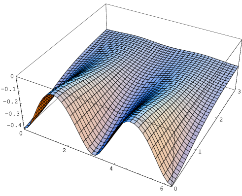
Figure 1: The behavior of the effective potential (19) for $(\beta/2\pi,ML)=(0.1,1.0)$. The gauge group is $SU(2)$.

By evaluating the tree-level potential (33) and the second derivative of the effective potential with respect to $\theta$ and $v$ at the minimum (25), we obtain the masses for $A_{y}$ and $\Sigma$ in one-loop approximation. Contrary to the modes ${\bar{A}}_{y}^{a=3}$ and ${\bar{\Sigma}}^{a=3}$, there arises the mass terms for ${\bar{A}}_{y}^{a=1,2}$ and ${\bar{\Sigma}}^{a=1,2}$ in the background (7) and (8) at the tree-level from the commutator between $A_{y}$ and $\Sigma$. It is calculated in the basis of $({\bar{A}}_{y}^{1},{\bar{A}}_{y}^{2},{\bar{\Sigma}}^{1},{\bar{\Sigma}}^{2})^{T}$ as

$${\cal M}_{tree}^{2}=\left(\begin{array}[]{cccc}4g^{2}v^{2}&0&-4\theta vg/L&0\\ 0&4g^{2}v^{2}&0&-4\theta vg/L\\ -4\theta vg/L&0&4\theta^{2}/L^{2}&0\\ 0&-4\theta vg/L&0&4\theta^{2}/L^{2}\end{array}\right).$$ (26)

The eigenvalues of the matrix are given by

$$0~{}(\mbox{degeneracy}=2,)\quad\mbox{and}\quad 4(g^{2}v^{2}+\theta^{2}/L^{2})~{}(\mbox{degeneracy}=2).$$ (27)

The two massless modes are the Nambu-Goldstone bosons absorbed by the charged massive gauge boson, and the rest corresponds to the charged massive state under the survived $U(1)$ gauge symmetry after the breakdown of the $SU(2)$ gauge symmetry.

The zero modes ${\bar{A}}_{y}^{a=3}$ and ${\bar{\Sigma}}^{a=3}$ become massive at the one-loop level. The masses are evaluated by the second derivative of the effective potential evaluated at the vacuum configuration (25)

$${\cal M}_{A_{y},\Sigma}^{2}=\left(\begin{array}[]{cc}{{\partial^{2}V_{eff}}\over{\partial\theta^{2}}}&{{\partial^{2}V_{eff}}\over{\partial\theta\partial v}}\\[8.5359pt] {{\partial^{2}V_{eff}}\over{\partial\theta\partial v}}&{{\partial^{2}V_{eff}}\over{\partial v^{2}}}\end{array}\right)_{vac}.$$ (28)

For the vacuum configuration, the off-diagonal elements vanish, so that the masses for ${\bar{A}}_{y}^{a=3},{\bar{\Sigma}}^{a=3}$ are given by $\frac{(gL)^{2}}{4}{{\partial^{2}V_{eff}}\over{\partial\theta^{2}}},\frac{1}{4}{{\partial^{2}V_{eff}}\over{\partial v^{2}}}$, respectively. Thus, we obtain that

$$m_{\Sigma}^{2} = \left({g_{4}\over L}\right)^{2}{{2\times 1}\over\pi^{2}}\sum_{n=1}^{\infty}{1\over n^{3}}\left[1-(1+nML){\rm e}^{-nML}\cos(n\beta)\right]\geq 0,$$ (29)

$$m_{A_{y}}^{2} = \left({g_{4}\over L}\right)^{2}{{2\times 3}\over\pi^{2}}\sum_{n=1}^{\infty}{1\over n^{3}}\left[1-(1+nML+{{(nML)^{2}}\over 3}){\rm e}^{-nML}\cos(n\beta)\right]\geq 0,$$ (30)

where we have defined the four dimensional gauge coupling $g_{4}\equiv g/\sqrt{L}$. The equality holds if and only if $\beta=2\pi{\bf Z}$ and $M=0$ are satisfied simultaneously, for which supersymmetry restores.

Let us first discuss the mass scale of $m_{A_{y},\Sigma}$. The mass scale of the generated mass is roughly estimated as

$$m_{\Sigma},~{}m_{A_{y}}\simeq cg_{4}\times\left\{\begin{array}[]{lll}1/L&\mbox{for}&ML\geq O(1),\\[8.5359pt] \mbox{max}~{}(M,~{}\beta/L)&\mbox{for}&ML<<1,\\[8.5359pt] \end{array}\right.$$ (31)

where $c$ is a numerical constant of order $O(1)$ and $\mbox{max}~{}(M,~{}\beta/L)$ stands for the larger scale among $M,\beta/L$. In order for ${\bar{A}}_{y},{\bar{\Sigma}}$ to become massive, one needs the breaking of both supersymmetry and the five dimensional local gauge invariance simultaneously. The former scale is given by the scale, $\mbox{max}~{}(M,~{}\beta/L)$, while the latter is given by the compactification scale $L^{-1}$. The mass scale should be the one at which both breaking are occurred. In fact, as observed in Eq.(31) the mass scale of $m_{A_{y},\Sigma}$ is the order of the scale at which the breaking is realized.

As the bare mass $M$ becomes larger and larger, the contribution from the fermion $\lambda_{D}$ to the effective potential is suppressed more and more thanks to the Boltzmann factor in Eq.(17), and what is left is the contribution from the boson alone. The parameter $\beta$ has no effect on the size of the mass in the heavy bare mass limit. The values of $\beta$ affects to the size of the mass for $ML\leq O(1)$. As shown in Table $1$, we see that $\beta/2\pi=0.5$, which corresponds to the antiperiodic boundary condition for the fermions and is the “maximal” breaking of supersymmetry, significantly enhances the masses. This is because for $\beta/2\pi=0.5$, the second term in Eqs.(29) and (30) becomes negative, and then, the contribution to the effective potential is additive to make the masses larger. It is important to study the supersymmetry breaking effect on the magnitude of the mass for the Higgs scalar in the scenario of the gauge-Higgs unification [21].

$\beta/2\pi$	${\bar{m}}_{A_{y}}(ML=1.0)$	${\bar{m}}_{\Sigma}(ML=1.0)$
$0.0$	0.503404	0.637422
$0.0001$	0.503404	0.637422
$0.001$	0.50343	0.637438
$0.01$	0.506036	0.63903
$0.1$	0.701635	0.771337
$0.5$	1.4134	1.37596
$\beta/2\pi$	${\bar{m}}_{A_{y}}(ML=0.1)$	${\bar{m}}_{\Sigma}(ML=0.1)$
$0.0$	0.0796115	0.119074
$0.0001$	0.079616	0.119076
$0.001$	0.0800608	0.119347
$0.01$	0.115059	0.143266
$0.1$	0.623837	0.62522
$0.5$	1.44998	1.44924

Table 1: The masses for $A_{y}$ and $\Sigma$ with respect to the values of $\beta/2\pi$ for fixed values of $ML=1.0$ and $0.1$. ${\bar{m}}_{A_{y}}\equiv{{m_{A_{y}}}\over{\left({g_{4}\over L}\right){{\sqrt{6}}\over\pi}}},~{}~{}{\bar{m}}_{\Sigma}\equiv{{m_{\Sigma}}\over{\left({g_{4}\over L}\right){{\sqrt{2}}\over\pi}}}$.

4 Conclusions and Discussions

We have studied the supersymmetric Yang-Mills theory on $M^{4}\times S^{1}$ by taking the two kinds of order parameter for the gauge symmetry breaking into account. One is the component gauge field $A_{y}$ for the $S^{1}$ direction, and the other one is the real scalar field $\Sigma$. The latter has been overlooked in the past. We have evaluated the effective potential for the order parameters in one-loop approximation. In the calculation we have employed the Scherk-Schwarz mechanism and have introduced the bare mass for $\lambda_{D}$ in order to break supersymmetry to yield the nonvanishing effective potential (19).

The effect of the vacuum expectation values $\Sigma$ and the bare mass $M$ appears as the Boltzmann suppression factor in the effective potential. This can be understood from the similarity of the potential with the one obtained in finite temperature field theory as explained in the text.

We have first studied the effective potential for the $SU(N)$ gauge group, and, by minimizing the potential, we have obtained the vacuum configuration (24), for which the gauge symmetry is not broken. We have also evaluated the masses for ${\bar{A}}_{y}^{a=3}$ and ${\bar{\Sigma}}^{a=3}$ by the second derivative of the effective potential at the vacuum configuration for the case of $SU(2)$. These masses are generated by the quantum effect due to the breaking of both supersymmetry and the five dimensional local gauge invariance. Hence, the mass scale should be the order of the scale at which both symmetries are violated, as evaluated in Eq.(31).

The suppression factor arising from $\langle\Sigma\rangle$ in the effective potential also appears for the case of orbifold compactification such as $S^{1}/Z_{2}$ [22][12][13]. This point has been overlooked in the past. As shown in the example, however, $\langle\Sigma\rangle$ takes the values of zero dynamically, and it is also the case for the orbifold compactification. And even if we introduce matter into the theory, we expect $\langle\Sigma\rangle=0$ at the minimum of the effective potential. Therefore, it is justified to consider the Wilson line phases alone, a posteriori, in evaluating the effective potential. It is more important to study the effect of the vacuum expectation values of squark field $\langle\phi_{i}\rangle$ in hypermultiplet and is interesting to find the case, where $\langle\phi_{i}\rangle$ take nontrivial values.

Acknowledgements

N.H. is supported in part by the Grant-in-Aid for Science Research, Ministry of Education, Science and Culture, Japan, No. 16540258, 16028214, 14740164. K.T. would thank the colleagues in Osaka University and the professor Y. Hosotani for valuable discussions, and he is supported by the $21$st Century COE Program at Osaka University. T.Y. would like to thank H.Kogetsu for useful discussion, and the Japan Society for the Promotion of Science for financial support.

Appendix

Equipped with the gauge fixing term (4) given in the text, the quadratic terms with respect to the fluctuations are given by

$${\cal L}_{eff}={\cal L}_{tree}+{\cal L}_{A_{\mu}}+{\cal L}_{A_{y}}+{\cal L}_{\Sigma}+{\cal L}_{\lambda_{D}}+{\cal L}_{others}$$ (32)

where

$${\cal L}_{tree} = g^{2}tr[\langle A_{y}\rangle,~{}\langle\Sigma\rangle]^{2},$$ (33)

$${\cal L}_{A_{\mu}} = -{1\over 2}tr(F_{\mu\nu}F^{\mu\nu})-g^{2}tr[{\bar{A}}_{\mu},~{}\langle\Sigma\rangle][{\bar{A}}^{\mu},~{}\langle\Sigma\rangle]$$ (34)

$$+ tr(D_{y}{\bar{A}}_{\mu})^{2}-{1\over\xi}tr(\partial_{\mu}{\bar{A}}^{\mu})^{2},$$

$${\cal L}_{A_{y}} = tr(\partial_{\mu}{\bar{A}}_{y})^{2}-\xi tr(D_{y}{\bar{A}}_{y})^{2}+g^{2}tr[{\bar{A}}_{y},~{}\langle\Sigma\rangle]^{2},$$ (35)

$${\cal L}_{\Sigma} = tr(D_{\hat{\mu}}{\bar{\Sigma}})^{2}+\xi g^{2}tr[\langle\Sigma\rangle,~{}{\bar{\Sigma}}]^{2},$$ (36)

$${\cal L}_{\lambda_{D}} = tr({\bar{\lambda}_{D}}i\Gamma^{\hat{\mu}}D_{\hat{\mu}}\lambda_{D}-g{\bar{\lambda}}_{D}[\langle\Sigma\rangle,~{}\lambda_{D}]),$$ (37)

$${\cal L}_{others} = 2ig(\xi-1)tr(D_{y}{\bar{A}}_{y}[\langle\Sigma\rangle,~{}{\bar{\Sigma}})]$$ (38)

$$- 2ig~{}tr(\partial_{\mu}{\bar{\Sigma}}[{\bar{A}}^{\mu},\langle\Sigma\rangle])-2ig~{}tr(\partial_{\mu}{\bar{A}}^{\mu}[\langle\Sigma\rangle,\bar{\Sigma}])$$

$$- 2g^{2}tr[\langle\Sigma\rangle,~{}\langle A_{y}\rangle][{\bar{\Sigma}},{\bar{A}}_{y}],$$

where the covariant derivative is defined in the background field $\langle A_{y}\rangle$ as,

$$D_{\hat{\mu}}\phi\equiv\partial_{\hat{\mu}}\phi-ig[\langle A_{\hat{\mu}}\rangle\delta_{\hat{\mu}y},~{}\phi],\qquad\phi\equiv{\bar{\Sigma}},~{}{\bar{A}}_{\mu},~{}{\bar{A}}_{y},~{}\lambda_{D}.$$ (39)

We see that $\xi=1$ gives a simple expression. For the background fields defined by (7) and (8), we obtain that

$${\cal L}_{\Sigma} = -tr{\bar{\Sigma}}\biggl{(}\partial_{\mu}\partial^{\mu}-(\partial_{y}-{i\over L}(\theta_{i}-\theta_{j}))^{2}+\xi g^{2}(v_{i}-v_{j})^{2}\biggr{)}{\bar{\Sigma}},$$ (40)

$${\cal L}_{A_{\mu}} = tr{\bar{A}}_{\mu}\biggl{(}\eta^{\mu\nu}[\partial_{\rho}\partial^{\rho}+g^{2}(v_{i}-v_{j})^{2}-(\partial_{y}-{i\over L}(\theta_{i}-\theta_{j}))^{2}]-(1-{1\over\xi})\partial^{\mu}\partial^{\nu}\biggr{)}{\bar{A}}_{\nu},$$ (41)

$${\cal L}_{A_{y}} = -tr{\bar{A}}_{y}\biggl{(}\partial_{\mu}\partial^{\mu}-\xi(\partial_{y}-{i\over L}(\theta_{i}-\theta_{j}))^{2}+g^{2}(v_{i}-v_{j})^{2}\biggr{)}{\bar{A}}_{y},$$ (42)

$${\cal L}_{\lambda_{D}} = tr{\bar{\lambda}}_{D}\left(i\Gamma^{\hat{\mu}}\partial_{\hat{\mu}}+\Gamma^{y}{1\over L}(\theta_{i}-\theta_{j})+g(v_{i}-v_{j})\right)\lambda_{D},$$ (43)

where $\xi=1$ is understood. Let us note that ${\cal L}_{others}$ vanishes for the parameterization of the vacuum expectation values (7) and (8) in the text.

References

• [1] Y. Hosotani, Phys. Lett. 126B (1983) 309, Ann. Phys. (N.Y.) 190, 233 (1989).
• [2] N. S. Manton, Nucl. Phys. B158 141 (1979), D. B. Fairlie, Phys. Lett. 82B (1979) 97.
• [3] N. V. Krasinikov, Phys. Lett. 273B (1991) 731, H. Hatanaka, T. Inami and C.S. Lim, Mod. Phys. Lett. A13 (1998) 2601, G. R. Dvali, S. Randjbar-Daemi and R. Tabbash, Phys. Rev. D65 (2002) 064021, N. Arkani-Hamed, A. G. Cohen and H. Georgi, Phys. Lett. 513B (2001) 232, I. Antiniadis, K. Benakli and M. Quiros, New J. Phys. 3, (2001),20.
• [4] M. Kubo, C. S. Lim and H. Yamashita, Mod. Phys. Lett. A17 (2002) 2249.
• [5] L. J. Hall, Y. Nomura and D. R. Smith, Nucl. Phys. B639 (2002) 307.
• [6] G. Burdman and Y. Nomura, Nucl. Phys. B656 (2002) 3.
• [7] N. Haba and Y. Shimizu, Phys. Rev. D67 (2003) 095001.
• [8] C. A. Scucca, M. Serone and L. Silvestrini, Nucl. Phys. B669 (2003) 128.
• [9] I. Gogoladze, Y. Mimura, S. Nandi and K. Tobe, Phys. Lett. 575B (2003) 66.
• [10] C. Csaki, C. Grojean, H. Murayama, L. Pilo and J. Terning, Phys. Rev. D69 (2004) 055006.
• [11] K. Choi, N. Haba, K. S. Jeong, K. Okumura, Y. Shimizu and M. Yamaguchi, J. High Energy Phys.0402, 037 (2004).
• [12] N. Haba, Y. Hosotani, Y. Kawamura and T. Yamashita, Phys. Rev. D70 (2004) 015010.
• [13] N. Haba and T. Yamashita, J. High Energy Phys.0404, 016 (2004).
• [14] Y. Hosotani, S. Noda and K. Takenaga, Phys. Rev. D69 (2004) 125014, [hep-ph/0410193].
• [15] A. T. Davies and A. McLachlan, Phys. Lett. 200B (1988) 305, Nucl. Phys. B317 237 (1989), J. E. Hetrick and C. L. Ho, Phys. Rev. D40 (1989) 4085, A. Higuchi and L. Parker, Phys. Rev. D37 (1988) 2853, C. L. Ho and Y. Hosotani, Nucl. Phys. B345 445 (1990), A. McLachlan, Nucl. Phys. B338 188 (1990), K. Takenaga, Phys. Rev. D64 (2001) 066001, Phys. Rev. D66 (2002) 085009.
• [16] M. Sohnius, Phys. Rep. 128, 39 (1985).
• [17] J. Scherk and J.H. Schwarz, Phys. Lett. 82B (1979) 60, P. Fayet, Phys. Lett. 159B (1985) 121, Nucl. Phys. B263 87 (1986), K. Takenaga, Phys. Lett. 425B (1998) 114, Phys. Rev. D58 (1998) 026004, D61 (2000) 129902(E).
• [18] K. Takenaga, Phys. Lett. 570B (2003) 244.
• [19] A. Delgado, A. Pomarol and M. Quiros, Phys. Rev. D60 (1999) 095008.
• [20] N. Haba, K. Takenaga and T. Yamashita, [hep-th/0410244].
• [21] N. Haba, K. Takenaga and T. Yamashita, [hep-ph/0411250].
• [22] N. Haba and T. Yamashita, J. High Energy Phys.02, 059 (2004).