ON THE THEORY OF INTERACTING FIELDS
IN FOLDY-WOUTHUYSEN REPRESENTATION

Abstract

The paper considers quantum electrodynamics (QED) and weak interaction of elementary particles in the lower orders of the perturbation theory using nonlocal Hamiltonian $H_{FW}$ in the Foldy-Wouthuysen ($FW$) representation. Feynman rules in the $FW$ representation are specified, specific QED processes are calculated. Cross sections of Coulomb scattering of electrons, Möller scattering, Compton effect, electron self-energy, vacuum polarization, anomalous magnetic moment of electron, Lamb shift of atomic energy levels are calculated. The possibility of the scattering matrix expansion in powers of the coupling constant, in which matrix elements $S_{fi}$ contain no terms with fermion propagators, is demonstrated for external fermion lines corresponding to real particles (antiparticles).

It is shown that a method to include the interaction of real particles with antiparticles in the $FW$ representation is to introduce negative mass particles and antiparticles to the theory. The theory is degenerate with respect to the particle (antiparticle) mass sign, however the masses of the particle and antiparticle interacting with each other should be of opposite sign.

QED in the $FW$ representation is invariant under $C$, $P$, $T$ inversions. The weak interaction breaks the $C$ and $P$ invariance, but preserves the combined $CP$ parity. In the theory there is a possibility to relate the break of $CP$ invariance to total or partial removal of the degeneracy in particle (antiparticle) mass sign.

INTRODUCTION

Historically, the first equation describing the $\displaystyle\frac{1}{2}$-spin particle with electromagnetic field has been non-relativistic Pauli equation

$$p_{0}\varphi\left({x}\right)=\left[{\displaystyle\frac{{\left({\vec{p}-e\vec{A}\left({x}\right)}\right)^{2}}}{{2m}}-\displaystyle\frac{{e\vec{\sigma}\vec{B}}}{{2m}}+eA_{0}\left({x}\right)}\right]\varphi\left({x}\right)$$ (1)

In (1) and hereinafter the system of units $\hbar=c=1$ is used; $x$, $p$, $A$ are 4-vectors; $xy=\linebreak=x^{\mu}y_{\mu}=x^{0}y^{0}-x^{k}y^{k}$, $\mu=0,1,2,3$, $k=1,2,3$ as usual; $p^{\mu}=i\displaystyle\frac{{\partial}}{{\partial x^{\mu}}}$; $\vec{B}=rot\vec{A}$; $\sigma^{k}$ are Pauli matrices; $\varphi\left({x}\right)$ is a two-component wave function.

Then Dirac derived his famous relativistic equation describing the $\displaystyle\frac{1}{2}$-spin particle motion. Given the interaction with magnetic field, the Dirac equation takes the form:

$$p_{0}\psi_{D}\left({x}\right)=\left[{\vec{\alpha}\left({\vec{p}-e\vec{A}\left({x}\right)}\right)+\beta m+eA_{0}\left({x}\right)}\right]\psi_{D}\left({x}\right),$$ (2)

$\psi_{D}\left({x}\right)$ — is the four-component wave function, $\alpha^{i}=\left({\begin{array}[]{cc}0&\sigma^{i}\\ \sigma^{i}&0\end{array}}\right)$, $\beta=\left({\begin{array}[]{cc}I&0\\ 0&-I\end{array}}\right)$ are the Dirac matrices. The Dirac equation, unlike equation (1), is linear in components of impulse $p^{\mu}$ and is readily representable in the explicitly covariant form. The Pauli equation is a nonrelativistic limit of the Dirac equation for the upper components of the wave function $\psi_{D}\left({x}\right)$.

In principle, the relativistic generalization of the Pauli equation could be performed in a different way with using the relativistic relation between energy and particle impulse as a basis when there are no external fields. This was actually done by Foldy and Wouthuysen in their classic paper [1]. The Foldy-Wouthuysen equation for free motion is

$$p_{0}\psi_{FW}\left({x}\right)=\left({H_{0}}\right)_{FW}\Psi_{FW}\left({x}\right)=\beta E\Psi_{FW}\left({x}\right)$$ (3)

In (3) $E=\sqrt{\vec{p}^{\,2}+m^{2}}$.

Solutions to (3) are plane waves of positive and negative energies

$$\psi_{FW}^{\left({+}\right)}\left({x,s}\right)=\displaystyle\frac{{1}}{{\left({2\pi}\right)^{3/2}}}U_{s}e^{-ipx},\quad\psi_{FW}^{\left({-}\right)}\left({x,s}\right)=\displaystyle\frac{{1}}{{\left({2\pi}\right)^{3/2}}}V_{s}e^{ipx},\quad p_{0}=\left({\vec{p}^{\,2}+m^{2}}\right)^{1/2}$$ (4)

In (4) $U_{s}=\left(\begin{array}[]{c}\chi_{s}\\ 0\end{array}\right)$, $V_{s}=\left(\begin{array}[]{c}0\\[-2.0pt] \chi_{s}\end{array}\right)$, $\chi_{s}$ are two-component normalized Pauli spin functions.

The following orthonormalization-completeness relationships are valid for $U_{s}$ and $V_{s}$:

$$\begin{array}[]{l}U_{s}^{+}U_{s^{{}^{\prime}}}=V_{s}^{+}V_{s^{{}^{\prime}}}=\delta_{ss^{{}^{\prime}}};\quad U_{s}^{+}V_{s^{{}^{\prime}}}=V_{s}^{+}U_{s^{{}^{\prime}}}=0;\\ \displaystyle\sum\limits_{s}{}\left({U_{s}}\right)_{\gamma}\left({U_{s}^{+}}\right)_{\delta}=\displaystyle\frac{{1}}{{2}}\left({I+\beta}\right)_{\gamma\delta};\quad\displaystyle\sum\limits_{s}{}\left({V_{s}}\right)_{\gamma}\left({V_{s}^{+}}\right)_{\delta}=\displaystyle\frac{{1}}{{2}}\left({I-\beta}\right)_{\gamma\delta}.\\ \end{array}$$ (5)

In (4), (5) $\gamma,\delta$ refer to the spinor subscripts, $s$ to the spin ones. In (5) and below the summation symbol and the subscripts themselves are omitted in the summation over the spinor subscripts.

Hamiltonian $\left({H_{0}}\right)_{FW}$ is related with free Dirac Hamiltonian $\left({H_{0}}\right)_{D}$ by the unitary transformation. In equation (3) definite asymmetry of space coordinates and time is seen, although it is Lorentz-invariant by itself.

In the general case of the interaction with external electromagnetic field $A^{\mu}\left({x}\right)$ there is no exact unitary transformation that would transform Dirac equation (2) to Foldy-Wouthuysen $\left({FW}\right)$ representation. In this case Foldy and Wouthuysen found Hamiltonian $\left({H_{FW}}\right)$ in the form of series in terms of powers of $1/m$ [1].

Blount [2] found Hamiltonian $\left({H_{FW}}\right)$ in the form of series in terms of powers of the smallness of fields and their time and space derivatives. Case [3] obtained an accurate transformation in the presence of time-independent external magnetic field $\vec{B}=rot\vec{A}$. In this case the Dirac equation is transformed to equation

$$p_{0}\psi_{FW}\left({x}\right)=H_{FW}\psi_{FW}\left({x}\right)=\beta\sqrt{\left({\vec{p}-e\vec{A}}\right)^{2}-e\vec{\sigma}\vec{B}+m^{2}}\cdot\psi_{FW}\left({x}\right).$$ (6)

The author obtains the relativistic Hamiltonian $\left({H_{FW}}\right)$ in the form of series in terms of powers of charge $e$ in the general case of interaction with external field $A^{\mu}\left({x}\right)$ [4].

In all the cases considered, in the Foldy-Wouthuysen representation the equations for wave functions are of noncovariant form and their Hamiltonians are nonlocal. In the $FW$ representation there is no relation between the upper and lower wave function components, that is, $H_{FW}$ is essentially a two-component Hamiltonian.

With the advent of the relativistic Hamiltonian $\left({H_{FW}}\right)$ obtained in ref. [4], it became possible to consider the $FW$ representation of quantum-field processes in the context of the perturbation theory. Why is it interesting irrespective of the non-covariance of the Dirac equation in the Foldy-Wouthuysen representation, nonlocality, and relative complexity of the expressions for Hamiltonian?

First, a number of paradoxes characteristic of the Dirac representation are resolved in the $FW$ representation. In the $FW$ representation, in the free case, the velocity operator is of habitual form $\vec{V}=\displaystyle\frac{{\vec{p}}}{{E}}$, which is close to the classic form (in the Dirac representation, $\vec{V}=\vec{\alpha}$), there is no electron ”jitter” (Zitterbewegung), the spin operator remains unchanged in time [1].

Second, since in Hamiltonian $H_{FW}$ there is no relation of the initial (final) states to positive energy and of final (initial) states to negative energy, in the quantum field theory there will be no interactions of real particle-antiparticle pairs. To include these processes, additional terms must be introduced to the Hamiltonian $H_{FW}$.

In this connection the consideration of the quantum field theory in the $FW$ representation can lead to new physical consequences and re-interpretation of the habitual terms in the Dirac representation.

Section 1 of this paper is devoted to quantum electrodynamics in the Foldy-Wouthuysen representation. Here Hamiltonian $H_{FW}$ is given in the form of series in terms of powers of $e$, Feynman rules in the$FW$ representation are specified, results of calculations of specific QED processes are discussed. For the case, where the external fermion lines correspond to real particles (antiparticles), the possibility of the scattering matrix expansion in powers of $e$, in which scattering matrix elements S_fi contain no terms with electron-positron propagators, is demonstrated.

The formulas for vertex operators are therewith close in their structure to those of the ”old”, noncovariant perturbation theory developed by Heitler [5].

Next, Section 1 demonstrates that a method to include the external electron-positron pair interaction in the $FW$ representation is to introduce the relationship between the solutions to the $FW$-transformed Dirac equations with positive and negative particle (antiparticle) mass. In so doing the positive-mass particles (antiparticles) interact with one another and with negative-mass antiparticles (particles). Conversely, negative-mass particles (antiparticles) interact with one another and with positive-mass antiparticles (particles). The theory is degenerate with respect to the particle (antiparticle) mass sign, however the masses of the particle and antiparticle interacting with each other should be of opposite signs. It should be particularly emphasized that in the context under discussion the particle mass sign is an internal quantum number not related by the author in this paper to the gravitational interaction sign. Of course, the negative-mass particle energy is therewith positive. Note that previously the conclusion of the opposite signs in the particle and antiparticle masses was made by Recami and Ziino [6] when analyzing the special relativity theory and conditions of reversibility ”particle $\leftrightarrow$ antiparticle”. The suggested form of QED in the $FW$ representation is invariant under $P,C,T$ transformations.

Section 2 is devoted to the theory of weak interaction in the $FW$representation. The weak interaction is considered in the lower order of the perturbation theory, in the $V$-$A$ form of the four-fermion interaction. The weak current in the $FW$ representation is determined explicitly. Like in the Dirac representation, weak interactions break the $P$ and $C$ invariance, but preserve the combined $CP$ parity. In the theory there is a possibility to relate the $CP$ invariance break to the partial removal of the degeneracy in particle (antiparticle) mass sign.

1 QUANTUM ELECTRODYNAMICS IN THE
FOLDY-WOUTHUYSEN REPRESENTATION
[4], [7], [8]

1.1 Interaction Hamiltonian in the $FW$ representation

In notation of ref. [4] Dirac equation for quantized electron-positron field in the $FW$ representation is written as

$$\begin{array}[]{l}p_{0}\psi_{FW}\left({x}\right)=H_{FW}\psi_{FW}\left({x}\right)=\left({\beta E+K_{1}+K_{2}+K_{3}+\ldots}\right)\psi_{FW}\left({x}\right),\\ K_{1}\sim e,\quad K_{2}\sim e^{2},\quad K_{3}\sim e^{3}.\end{array}$$ (7)

In the impulse representation, with electromagnetic field expansion in plane waves

$$A_{\mu}\left({\vec{x},t}\right)=\sum\limits_{\nu=\pm 1}{}\int{A_{\mu k}^{\left({\nu}\right)}e^{i\nu k_{o}t}e^{-i\vec{k}\vec{x}}d\vec{k}}$$

matrix elements of interaction Hamiltonian terms $K_{1},K_{2}$ can be written as

$$\langle\vec{p}^{\,{}^{\prime}}\left|{K_{1}}\right|{\kern 1.0pt}\vec{p}^{\prime\prime}\rangle=\sum\limits_{\nu=\pm 1}{}\displaystyle\frac{{\beta E^{{}^{\prime\prime}}-\beta E^{{}^{\prime}}-\nu k_{0}}}{{R^{{}^{\prime}}+R^{{}^{\prime\prime}}}}\left({-\displaystyle\frac{{1}}{{\beta E^{{}^{\prime}}+\beta E^{{}^{\prime\prime}}-\nu k_{0}}}\langle\vec{p}^{\,{}^{\prime}}\left|{RLN}\right|\vec{p}^{\,{}^{\prime\prime}}\rangle-}\right.$$

$$\left.-\displaystyle\frac{{1}}{{\beta E^{{}^{\prime}}+\beta E^{{}^{\prime\prime}}+\nu k_{0}}}\langle\vec{p}^{\,{}^{\prime}}\left|{NLR}\right|\vec{p}^{\,{}^{\prime\prime}}\rangle\right)+\langle\vec{p}^{\,{}^{\prime}}\left|C\right|\vec{p}^{\,{}^{\prime\prime}}\rangle;$$ (8)

$$\langle\vec{p}^{\,{}^{\prime}}\left|{K_{2}}\right|\vec{p}^{\,{}^{\prime\prime}}\rangle=\sum\limits_{\nu,\nu^{{}^{\prime}}=\pm 1}{}\int{d\vec{p}^{\,{}^{\prime\prime\prime}}\left\{{\displaystyle\frac{{\beta E^{{}^{\prime\prime}}-\beta E^{{}^{\prime}}-\nu k_{0}-\nu^{{}^{\prime}}k_{0}^{{}^{\prime}}}}{{R^{{}^{\prime}}+R^{{}^{\prime\prime}}}}\times}\right.}$$

$$\times\left[\displaystyle\frac{1}{\left({\beta E^{{}^{\prime}}+\beta E^{{}^{\prime\prime\prime}}-\nu k_{0}}\right)\left({\beta E^{{}^{\prime\prime}}-\beta E^{{}^{\prime\prime\prime}}-\nu^{{}^{\prime}}k_{0}^{{}^{\prime}}}\right)}\right.\langle\vec{p}^{\,{}^{\prime}}\left|R\left({C+\xi}\right)\right|\vec{p}^{\,{}^{\prime\prime\prime}}\rangle\langle\vec{p}^{\,{}^{\prime\prime\prime}}\left|K_{1}\right|\vec{p}^{\,{}^{\prime\prime}}\rangle+$$

$$+\displaystyle\frac{1}{\left({\beta E^{{}^{\prime\prime}}+\beta E^{{}^{\prime\prime\prime}}+\nu^{{}^{\prime}}k_{0}^{{}^{\prime}}}\right)\left({\beta E^{{}^{\prime\prime\prime}}-\beta E^{{}^{\prime}}-\nu k_{0}}\right)}\langle\vec{p}^{\,{}^{\prime}}\left|K_{1}\right|\vec{p}^{\,{}^{\prime\prime\prime}}\rangle\langle\vec{p}^{\,{}^{\prime\prime\prime}}\left|\left({C+\xi^{+}}\right)\left.{R}\right|\vec{p}^{\,{}^{\prime\prime}}\right.\rangle-$$

$$-\displaystyle\frac{1}{\left({\beta E^{{}^{\prime\prime}}+\beta E^{{}^{\prime}}-\nu k_{0}-\nu^{{}^{\prime}}k_{0}^{{}^{\prime}}}\right)\left({\beta E^{{}^{\prime\prime}}+\beta E^{{}^{\prime\prime\prime}}-\nu^{{}^{\prime}}k_{0}^{{}^{\prime}}}\right)}\langle\vec{p}^{\,{}^{\prime}}\left|R\left({N+\varphi}\right)\right|\vec{p}^{\,{}^{\prime\prime\prime}}\rangle\langle\vec{p}^{\,{}^{\prime\prime\prime}}\left|N\right|\vec{p}^{\,{}^{\prime\prime}}\rangle+$$

$$+\displaystyle\frac{1}{\left({\beta E^{{}^{\prime\prime}}+\beta E^{{}^{\prime}}+\nu k_{0}+\nu^{{}^{\prime}}k_{0}^{{}^{\prime}}}\right)\left({\beta E^{{}^{\prime\prime\prime}}+\beta E^{{}^{\prime}}+\nu k_{0}}\right)}\langle\vec{p}^{\,{}^{\prime}}\left|N\right|\vec{p}^{\,{}^{\prime\prime\prime}}\rangle\langle\vec{p}^{\,{}^{\prime\prime\prime}}\left|\left({N+\varphi^{+}}\right)R\right|\vec{p}^{\,{}^{\prime\prime}}\rangle-$$

$$-\displaystyle\frac{1}{\left({\beta E^{{}^{\prime\prime}}+\beta E^{{}^{\prime}}-\nu k_{0}-\nu^{{}^{\prime}}k_{0}^{{}^{\prime}}}\right)\left({\beta E^{{}^{\prime\prime}}-\beta E^{{}^{\prime\prime\prime}}-\nu^{{}^{\prime}}k_{0}^{{}^{\prime}}}\right)}\langle\vec{p}^{\,{}^{\prime}}\left|R\left({C+\xi}\right)\right|\vec{p}^{\,{}^{\prime\prime\prime}}\rangle\langle\vec{p}^{\,{}^{\prime\prime\prime}}\left|C\right|\vec{p}^{\,{}^{\prime\prime}}\rangle-$$

$$\left.-\displaystyle\frac{1}{\left({\beta E^{{}^{\prime\prime}}+\beta E^{{}^{\prime}}+\nu k_{0}+\nu^{{}^{\prime}}k_{0}^{{}^{\prime}}}\right)\left({\beta E^{{}^{\prime\prime\prime}}-\beta E^{{}^{\prime}}-\nu k_{0}}\right)}\langle\vec{p}^{\,{}^{\prime}}\left|C\right|\vec{p}^{\,{}^{\prime\prime\prime}}\rangle\langle\vec{p}^{\,{}^{\prime\prime\prime}}\left|\left({C+\xi^{+}}\right)R\right|\vec{p}^{\,{}^{\prime\prime}}\rangle\right]+$$

$$+\displaystyle\frac{1}{R^{{}^{\prime}}+R^{{}^{\prime\prime}}}\left[-\displaystyle\frac{{\beta E^{{}^{\prime\prime}}-\beta E^{{}^{\prime}}-\nu k_{0}-\nu^{{}^{\prime}}k_{0}^{{}^{\prime}}}}{{\left({\beta E^{{}^{\prime\prime\prime}}-\beta E^{{}^{\prime}}-\nu k_{0}}\right)\left({\beta E^{{}^{\prime\prime}}-\beta E^{{}^{\prime\prime\prime}}-\nu^{{}^{\prime}}k_{0}^{{}^{\prime}}}\right)}}\right.\langle\vec{p}^{\,{}^{\prime}}\left|RC\right|\vec{p}^{\,{}^{\prime\prime\prime}}\rangle\langle\vec{p}^{\,{}^{\prime\prime\prime}}\left|K_{1}\right|\vec{p}^{\,{}^{\prime\prime}}\rangle+$$

$$+\displaystyle\frac{\beta E^{{}^{\prime\prime}}-\beta E^{{}^{\prime}}-\nu k_{0}-\nu^{{}^{\prime}}k_{0}^{{}^{\prime}}}{\left({\beta E^{{}^{\prime\prime\prime}}-\beta E^{{}^{\prime}}-\nu k_{0}}\right)\left({\beta E^{{}^{\prime\prime}}-\beta E^{{}^{\prime\prime\prime}}-\nu^{{}^{\prime}}k_{0}^{{}^{\prime}}}\right)}\langle\vec{p}^{\,{}^{\prime}}\left|K_{1}\right|\vec{p}^{\,{}^{\prime\prime\prime}}\rangle\langle\vec{p}^{\,{}^{\prime\prime\prime}}\left|CR\right|\vec{p}^{\,{}^{\prime\prime}}\rangle+$$

$$+\displaystyle\frac{1}{\beta E^{{}^{\prime\prime\prime}}-\beta E^{{}^{\prime}}-\nu k_{0}}\langle\vec{p}^{\,{}^{\prime}}\left|RK_{1}\right|\vec{p}^{\,{}^{\prime\prime\prime}}\rangle\langle\vec{p}^{\,{}^{\prime\prime\prime}}\left|K_{1}\right|\vec{p}^{\,{}^{\prime\prime}}\rangle-$$

$$-\displaystyle\frac{1}{\beta E^{{}^{\prime\prime}}-\beta E^{{}^{\prime\prime\prime}}-\nu^{{}^{\prime}}k_{0}^{{}^{\prime}}}\langle\vec{p}^{\,{}^{\prime}}\left|K_{1}\right|\vec{p}^{\,{}^{\prime\prime\prime}}\rangle\langle\vec{p}^{\,{}^{\prime\prime\prime}}\left|K_{1}R\right|\vec{p}^{\,{}^{\prime\prime}}\rangle+$$

$$+\displaystyle\frac{1}{\beta E^{{}^{\prime\prime}}-\beta E^{{}^{\prime\prime\prime}}-\nu^{{}^{\prime}}k_{0}^{{}^{\prime}}}\langle\vec{p}^{\,{}^{\prime}}\left|RC\right|\vec{p}^{\,{}^{\prime\prime\prime}}\rangle\langle\vec{p}^{\,{}^{\prime\prime\prime}}\left|C\right|\vec{p}^{\,{}^{\prime\prime}}\rangle-$$

$$-\displaystyle\frac{1}{\beta E^{{}^{\prime\prime\prime}}-\beta E^{{}^{\prime}}-\nu k_{0}}\langle\vec{p}^{\,{}^{\prime}}\left|C\right|\vec{p}^{\,{}^{\prime\prime\prime}}\rangle\langle\vec{p}^{\,{}^{\prime\prime\prime}}\left|CR\right|\vec{p}^{\,{}^{\prime\prime}}\rangle+$$

$$+\displaystyle\frac{1}{\beta E^{{}^{\prime\prime}}+\beta E^{{}^{\prime\prime\prime}}-\nu^{{}^{\prime}}k_{0}^{{}^{\prime}}}\langle\vec{p}^{\,{}^{\prime}}\left|RN\right|\vec{p}^{\,{}^{\prime\prime\prime}}\rangle\langle\vec{p}^{\,{}^{\prime\prime\prime}}\left|N\right|\vec{p}^{\,{}^{\prime\prime}}\rangle+$$

$$\left.\left.+\displaystyle\frac{1}{\beta E^{{}^{\prime\prime\prime}}+\beta E^{{}^{\prime}}+\nu k_{0}}\langle\vec{p}^{\,{}^{\prime}}\left|N\right|\vec{p}^{\,{}^{\prime\prime\prime}}\rangle\langle\vec{p}^{\,{}^{\prime\prime\prime}}\left|NR\right|\vec{p}^{\,{}^{\prime\prime}}\rangle\right]\right\}.$$ (9)

In (1.1) $\xi=-\displaystyle\frac{{1}}{{R}}\left({A_{0}+\vec{\alpha}\vec{A}\displaystyle\frac{{\beta\vec{\alpha}\vec{p}}}{{E+m}}}\right)R,\qquad\varphi=\displaystyle\frac{{1}}{{R}}\left({A_{0}\displaystyle\frac{{\beta\vec{\alpha}\vec{p}}}{{E+m}}+\vec{\alpha}\vec{A}}\right)R$,
$\xi^{+},\varphi^{+}$ are operators Hermitean conjugate to $\xi,\varphi$.

In (1.1) and (9) operators $C,\,N,\,L,\,R$ are

$$\begin{array}[]{l}C=eR\left({A_{0}-LA_{0}L}\right)R-eR\left({L\vec{\alpha}\vec{A}-\vec{\alpha}\vec{A}L}\right)R,\\ N=eR\left({LA_{0}-A_{0}L}\right)R-eR\left({\vec{\alpha}\vec{A}-L\vec{\alpha}\vec{A}L}\right)R,\\ L=\displaystyle\frac{{\beta\vec{\alpha}\vec{p}}}{{E+m}},\quad R=\sqrt{\displaystyle\frac{{E+m}}{{2E}}}.\end{array}$$

The expressions for $C,\,R$ are even operators, that is the operators not relating the upper and lower components of wave functions $\Psi_{FW}\left({x}\right)$; accordingly, the expressions for $N,L$ are odd operators. The interaction Hamiltonian terms $K_{1},K_{2},\ldots$, as they must, are even operators.

An algorithm for determination of the $K_{1},K_{2}$ and the following terms of the expansion in powers of $e$ is given in ref. [4]. Appendix 1 of this paper briefly presents the algorithm for determination of Hamiltonian terms $K_{1}$, $K_{2}$, $K_{3}$.

1.2 Feynman rules in the $FW$ representation

The Feynman propagator of the Dirac equation in the Foldy-Wouthuysen representation is

$$S_{FW}\left({x-y}\right)=\displaystyle\frac{{1}}{{\left({2\pi}\right)^{4}}}\int{d^{4}p\displaystyle\frac{{e^{-i\rho\left({x-y}\right)}}}{{\rho_{0}-\beta E}}}=\displaystyle\frac{{1}}{{\left({2\pi}\right)^{4}}}\int{d^{4}p}e^{-i\rho\left({x-y}\right)}\displaystyle\frac{{p_{0}+\beta E}}{{p^{2}-m^{2}+i\varepsilon}}=$$

$$=-i\theta\left({x_{0}-y_{0}}\right)\int{d\vec{p}\sum\limits_{s}{\psi_{FW}^{\left({+}\right)}\left({x,s}\right)\left({\psi_{FW}^{\left({+}\right)}\left({y,s}\right)}\right)}}^{+}+$$

$$+i\theta\left({y_{0}-x_{0}}\right)\int{d\vec{p}\sum\limits_{s}{\psi_{FW}^{\left({-}\right)}\left({x,s}\right)\left({\psi_{FW}^{\left({-}\right)}\left({y,s}\right)}\right)}}^{+}.$$ (10)

Eq. (1.2) implies the Feynman rule of pole bypass; $\theta\left({x_{0}}\right)=\left\{\begin{array}[]{ll}1,&x_{0}>0;\\ 0,&x_{0}<0.\end{array}\right.$

The integral equation for $\psi_{FW}\left({x}\right)$ is

$$\psi_{FW}\left({x}\right)=\psi_{0}\left({x}\right)+\int{d^{4}yS_{FW}\left({x-y}\right)\left({K_{1}+K_{2}+\ldots}\right)\psi_{FW}\left({y}\right)}.$$ (11)

In (11) $\psi_{0}\left({x}\right)$ is the solution to the Dirac equation in the $FW$representation in the absence of electromagnetic field $\left({A^{\mu}=0}\right).$

Expressions (1.2), (11) allow us to formulate the Feynman rules for recording elements of scattering matrix $S_{fi}$ and calculating QED processes. In contrast to the Dirac representation, in the FW representation there is an infinite set of types of photon interaction vertices depending on the perturbation theory order: the vertex of interaction with one photon is correspondent with factor $\left({-i(K_{1})_{\mu}}\right)$, the vertex of interaction with two photons with factor $\left({-i(K_{2})_{\mu\nu}}\right)$ and so on. For convenience the corresponding parts of the terms of interaction Hamiltonian $K_{1},K_{2},\ldots$ without electromagnetic potentials $A^{\mu},A^{\mu}A^{\nu},\ldots$ are denoted by $(K_{1})_{\mu},(K_{2})_{\mu\nu},\ldots$.

Each external fermion line is correspondent with one of functions (4). As usually, positive energy solutions correspond to particles, negative energy solutions to antiparticles. The other Feynman rules remain the same as those in the spinor electrodynamics in the Dirac representation.

1.3 Calculations of QED processes in the $FW$ representation

The formulated Feynman rules have been used to consider some QED processes in the first and second orders of the perturbation theory. Cross sections of Coulomb scattering of electrons, Möller scattering, Compton effect, electron self-energy, vacuum polarization, anomalous magnetic moment of electron, Lamb shift of atomic energy levels have been calculated. Below are given the Feynman diagrams of the processes considered. The brief details of the calculations can be found in Appendix 2.

The final results of calculations of the QED processes, whose diagrams are presented in Figs. 1—5, agree with the relevant data calculated in the Dirac representation. The radiation corrections to the electron scattering in the external field (Fig. 6) in the mass and charge renormalization provide a proper value of the anomalous magnetic electron and Lamb shift of energy levels.

A feature of the theory is that in the terms of the interaction Hamiltonian $K_{n}$ (except $K_{1}$) there is an even number N of odd operators relating the initial and final states of positive energy to the intermediate states of negative energy and vice versa. Thanks to this, for example, the diagram of Fig. 5 appears that relates to the electron-positron vacuum polarization. In this theory there is no habitual diagram for the vacuum polarization with two vertices of the first order in $e$ because operator $K_{1}$ is even.

When the external fermion line impulses lie on the mass surface $\left({p^{2}=m^{2}}\right)$, an interesting feature of the theory is the compensation of the contribution of the fermion propagator diagrams with that of the relevant terms in the diagrams with vertices of the higher order of the expansion in e. Thus, in Fig. 3 the contribution of diagrams a) and c) is compensated with the relevant parts of the contribution of diagrams b) and d); the contribution of diagram a) in Fig. 4 is cancelled with the contribution of the corresponding part of diagram b); in Fig. 6 the contribution of diagrams a), b), c) is cancelled with that of the corresponding part of diagram d), a similar compensation occurs for diagrams e), f), g) and h); i), j), k) and l), respectively. For the real external fermions under discussion the vertex operators $K_{n}$ get therewith simplified significantly because of the law of conservation of energy-momentum (see, e. g., (1.1), (1.1)).

In view of the aforesaid, the scattering matrix can be expanded in powers of e so, that the matrix elements $S_{fi}$ contain no terms with electron-positron propagators. In so doing the vertex operator matrix elements alter as follows:

$$\!\!\!\!\!\!\!\!\!\!\langle\vec{p}^{\,{}^{\prime}}\left|{K_{1}}\right|\vec{p}^{\,{}^{\prime\prime}}\rangle\to\langle\vec{p}^{\,{}^{\prime}}\left|{C}\right|\vec{p}^{\,{}^{\prime\prime}}\rangle;$$ (12)

$$\!\!\!\!\!\!\!\!\!\!\langle\vec{p}^{\,{}^{\prime}}\left|{K_{2}}\right|\vec{p}^{\,{}^{\prime\prime}}\rangle\to\sum\limits_{\nu_{2}=\pm 1}{\int{d\vec{p}^{\,{}^{\prime\prime\prime}}\left\{{\displaystyle\frac{{1}}{{\beta E^{{}^{\prime\prime}}-\beta E^{{}^{\prime\prime\prime}}-\nu_{2}k_{2}^{0}}}\langle\vec{p}^{\,{}^{\prime}}\left|{C}\right|\vec{p}^{\,{}^{\prime\prime\prime}}\rangle\langle\vec{p}^{\,{}^{\prime\prime\prime}}\left|{C}\right|\vec{p}^{\,{}^{\prime\prime}}\rangle+}\right.}}$$

$$\!\!\!\!\!\!\!\!\!\!+\left.\displaystyle\frac{{1}}{{\beta E^{{}^{\prime\prime}}+\beta E^{{}^{\prime\prime\prime}}-\nu_{2}k_{2}^{0}}}\langle\vec{p}^{\,{}^{\prime}}\left|{N}\right|\vec{p}^{\,{}^{\prime\prime\prime}}\rangle\langle\vec{p}^{\,{}^{\prime\prime\prime}}\left|{N}\right|\vec{p}^{\,{}^{\prime\prime}}\rangle\right\};$$ (13)

$$\!\!\!\!\!\!\!\!\!\!\langle\vec{p}^{\,{}^{\prime}}\left|{K_{3}}\right|\vec{p}^{\,{}^{\prime\prime}}\rangle\to\sum\limits_{\nu_{1}\nu_{2}=\pm 1}{\int{d\vec{p}^{\,{}^{\prime\prime\prime}}d\vec{p}^{\,IV}\displaystyle\frac{{1}}{{\left({\beta E^{IV}-\beta E^{{}^{\prime}}-\nu_{1}k_{1}^{0}-\nu_{2}k_{2}^{0}}\right)\left({\beta E^{{}^{\prime\prime\prime}}-\beta E^{{}^{\prime}}-\nu_{1}k_{1}^{0}}\right)}}}\times}$$

$$\!\!\!\!\!\!\!\!\!\!\times\langle\vec{p}^{\,{}^{\prime}}\left|{C}\right|\vec{p}^{\,{}^{\prime\prime\prime}}\rangle\langle\vec{p}^{\,{}^{\prime\prime\prime}}\left|{C}\right|\vec{p}^{\,IV}\!\!\rangle\langle\vec{p}^{\,IV}\!\!\left|{C}\right|\vec{p}^{\,{}^{\prime\prime}}\rangle-\displaystyle\frac{{1}}{{\left({\beta E^{IV}+\beta E^{{}^{\prime}}+\nu_{1}k_{1}^{0}+\nu_{2}k_{2}^{0}}\right)\left({\beta E^{{}^{\prime\prime\prime}}-\beta E^{{}^{\prime}}-\nu_{1}k_{1}^{0}}\right)}}\times$$

$$\!\!\!\!\!\!\!\!\!\!\times\langle\vec{p}^{\,{}^{\prime}}\left|{C}\right|\vec{p}^{\,{}^{\prime\prime\prime}}\rangle\langle\vec{p}^{\,{}^{\prime\prime\prime}}\left|{N}\right|\vec{p}^{\,IV}\!\!\rangle\langle\vec{p}^{\,IV}\!\!\left|{N}\right|\vec{p}^{\,{}^{\prime\prime}}\rangle+\displaystyle\frac{{1}}{{\left({\beta E^{IV}+\beta E^{{}^{\prime}}+\nu_{1}k_{1}^{0}+\nu_{2}k_{2}^{0}}\right)\left({\beta E^{{}^{\prime\prime\prime}}+\beta E^{{}^{\prime}}+\nu_{1}k_{1}^{0}}\right)}}\times$$

$$\!\!\!\!\!\!\!\!\!\!\times\langle\vec{p}^{\,{}^{\prime}}\left|{N}\right|\vec{p}^{\,{}^{\prime\prime\prime}}\rangle\langle\vec{p}^{\,{}^{\prime\prime\prime}}\left|{C}\right|\vec{p}^{\,IV}\!\!\rangle\langle\vec{p}^{\,IV}\!\!\left|{N}\right|\vec{p}^{\,{}^{\prime\prime}}\rangle-\displaystyle\frac{{1}}{{\left({\beta E^{IV}-\beta E^{{}^{\prime}}-\nu_{1}k_{1}^{0}-\nu_{2}k_{2}^{0}}\right)\left({\beta E^{{}^{\prime\prime\prime}}+\beta E^{{}^{\prime}}+\nu_{1}k_{1}^{0}}\right)}}\times$$

$$\!\!\!\!\!\!\!\!\!\!\times\langle\vec{p}^{\,{}^{\prime}}\left|{N}\right|\vec{p}^{\,{}^{\prime\prime\prime}}\rangle\langle\vec{p}^{\,{}^{\prime\prime\prime}}\left|{N}\right|\vec{p}^{\,IV}\!\!\rangle\langle\vec{p}^{\,IV}\!\!\left|{C}\right|\vec{p}^{\,{}^{\prime\prime}}\rangle.$$ (14)

Relations (1.3), (1.3) are close in their structure to the formulas of the “old”, noncovariant perturbation theory developed by Heitler in the Dirac representation [5]. Expressions (1.3), (1.3) can be derived from the relations of the Heitler’s perturbation theory, if the FW transformation is performed for the free case of $A^{\mu}\left({x}\right)=0$ in the matrix elements of the Heitler’s quantities $\left({K_{n}}\right)$ (therewith $\alpha_{\mu}A^{\mu}\left({x}\right)\,\to\,\left({C+N}\right)$) and nonzero terms (even in the upper and lower components of states $\langle\left.{A_{FW}}\right|$ and $\left|{B_{FW}\rangle}\right.$) are left in products $\langle A_{FW}\left|{\left({C+N}\right)\left({C+N}\right)\ldots}\right|B_{FW}\rangle$ that have appeared. It seems that this rule can be extended to the higher terms of the expansion in e as well.

A significant difference of expressions (1.3), (1.3), etc. from the formulas of ref. [5] is absence of any interaction between real electrons and positrons because the Hamiltonian in the FW representation is even. In this representation the electron-positron interaction can be only between the real and intermediate virtual states.

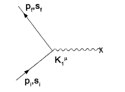
Figure 1: Electron scattering in Coulomb field

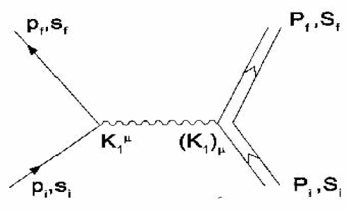
Figure 2: Electron scattering on Dirac proton (Möller scattering)

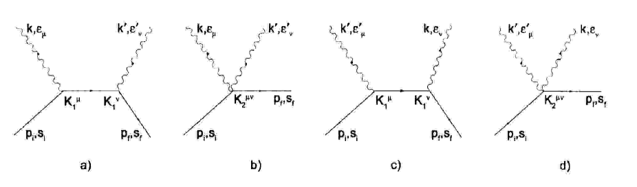
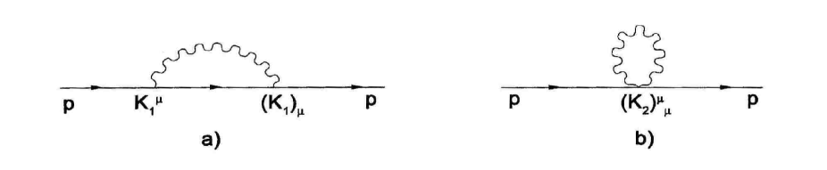
Figure 3: Compton effect

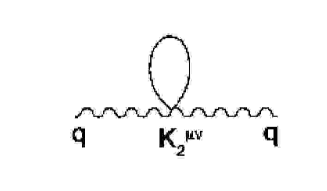
Figure 4: Electron self-energy

Figure 5: Vacuum polarization

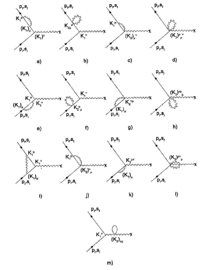
Figure 6: Radiation corrections to the electron scattering in the external field

1.4 Inclusion of electron-positron pair interactions
in the $FW$ representation

To construct real particle-antiparticle pair interaction processes in the theory, additional terms must be introduced to Hamiltonian H_FW. A method to include processes with real electron-positron pairs that would ensure proper results in the calculation of QED effects (for example, electron-positron pair annihilation cross section) is to introduce interaction between positive-energy (negative-energy) states of equation (7) and negative-energy (positive-energy) states of equation (15) derived by the FW transformation of Dirac equation (2) with negative particle mass.

$$p_{0}\psi_{1FW}\left({x}\right)=\left[{\beta E+K_{1}\left({-m}\right)+K_{2}\left({-m}\right)+\ldots}\right]\psi_{1FW}\left({x}\right).$$ (15)

Equation (7) with the additional interaction can be written as

$$\begin{array}[]{l}p_{0}\psi_{FW}\left({x}\right)=\beta E\psi_{FW}\left({x}\right)+\Bigg{[}{K_{1}\left({m,I,m}\right)}+\\ +\left.\displaystyle\frac{{1}}{{2}}K_{2}\left({m,I,m;m,I,m}\right)+\displaystyle\frac{{1}}{{2}}K_{2}\left({m,\gamma_{5},-m;-m,\gamma_{5},m}\right)+\ldots\right]\psi_{FW}\left({x}\right)+\\ +\left[K_{1}\left(m,\gamma_{5},-m\right)+\displaystyle\frac{{1}}{{2}}K_{2}\left({m,\gamma_{5},-m;-m,I,-m}\right)+\right.\\ \left.+\displaystyle\frac{{1}}{{2}}K_{2}\left({m,I,m;m,\gamma_{5},-m}\right)+\ldots\right]\psi_{1FW}\left({x}\right)\end{array}$$ (16)

In equation (16), the notation of terms $K_{1},K_{2},\ldots$ indicates the presence or absence of matrix $\gamma_{5}$ near potentials $A^{\mu}\,\left({x}\right)$ and the mass sign on the left or on the right of fields $A^{\mu}\,\left({x}\right)$. Factor $\displaystyle\frac{1}{2}$ of terms K₂ is introduced because of two possible ways of transition to the final state of mass +m. Similar to (16), the additional terms of interaction with field $\psi_{FW}\left({x}\right)$ can be introduced to equation (15) with negative mass.

The considered interaction between equations (7), (15) can be formalized as follows. Introduce eight-component field $\Phi_{FW}\left({x}\right)$, in which the four upper components are solutions to equation (7) with positive mass $\left({+m}\right)$ and the lower components are solutions to equation (15) with negative mass $\left({-m}\right)$. In the case under discussion solutions (4) for free motion are written as

$$\Phi_{FW}^{\left({+}\right)}\left({x,s,+m}\right)=\displaystyle\frac{{1}}{{\left({2\pi}\right)^{3/2}}}\left({\begin{array}[]{c}{U_{s}}\\ {0}\end{array}}\right)e^{-ipx};$$

$$\Phi_{FW}^{\left({+}\right)}\left({x,s,-m}\right)=\displaystyle\frac{{1}}{{\left({2\pi}\right)^{3/2}}}\left({\begin{array}[]{c}{0}\\ {U_{s}}\end{array}}\right)e^{-ipx};$$

$$\Phi_{FW}^{\left({-}\right)}\left({x,s,+m}\right)=\displaystyle\frac{{1}}{{\left({2\pi}\right)^{3/2}}}\left({\begin{array}[]{c}{V_{s}}\\ {0}\end{array}}\right)e^{ipx};$$

$$\Phi_{FW}^{\left({-}\right)}\left({x,s,-m}\right)=\displaystyle\frac{{1}}{{\left({2\pi}\right)^{3/2}}}\left({\begin{array}[]{c}{0}\\ {V_{s}}\end{array}}\right)e^{ipx}.$$

The extension of orthonormalization and completeness relations (5) to eight dimensions is quite evident.

Next, introduce matrices $8\times 8$:

$$\beta_{1}=\left(\begin{array}[]{cc}I&0\\ 0&-I\end{array}\right),\quad\rho=\left(\begin{array}[]{cc}0&\gamma_{5}\\ \gamma_{5}&0\end{array}\right),$$

$$\alpha^{k}=\left(\begin{array}[]{cc}\alpha^{k}&0\\ 0&\alpha^{k}\end{array}\right),\quad\sigma^{k}=\left(\begin{array}[]{cc}\sigma^{k}&0\\ 0&\sigma^{k}\end{array}\right),\quad\beta=\left(\begin{array}[]{cc}\beta&0\\ 0&\beta\end{array}\right).$$

$$\beta_{1}^{2}=\rho^{2}=I;\quad[\beta_{1},\rho]_{+}=[\beta,\rho]_{+}=0;$$

$$[\beta_{1},\alpha^{k}]_{-}=[\beta_{1},\sigma^{k}]_{-}=[\beta_{1},\beta]_{-}=0;$$

$$[\rho,\alpha^{k}]_{-}=[\rho,\sigma^{k}]_{-}=0.$$

Having substituted $m\to\beta_{1}m$, equations (7), (15) can be combined using the matrices $8\times 8$ as

$$p_{0}\Phi_{FW}\left({x}\right)=\Big{[}\beta E+K_{1}\left({\beta_{1}m,\left({I+\rho}\right),\beta_{1}m}\right)+$$

$$+\displaystyle\frac{1}{2}K_{2}\left({\beta_{1}m,\left({I+\rho}\right),\beta_{1}m;\beta_{1}m,\left({I+\rho}\right),\beta_{1}m}\right)+$$

$$\left.+\displaystyle\frac{1}{4}K_{3}\left({\beta_{1}m_{,}\left({I+\rho}\right),\beta_{1}m;\beta_{1}m,\left({I+\rho}\right),\beta_{1}m;\beta_{1}m,\left({I+\rho}\right),\beta_{1}m}\right)+\ldots\right]\Phi_{FW}\left({x}\right)$$ (18)

Equation (1.4) contains equation (16) for field $\psi_{FW}\left({x}\right)$ and relevant equation for field $\psi_{1FW}\left({x}\right)$. Interaction $\left({I+\rho}\right)A^{\mu}\left({x}\right)$ allows coupling between solutions (17$a$) and (17$d$), (17$b$) and (17$c$), while there is, as previously, no coupling between the other pairs of solutions, (17$a$) and (17$c$), (17$b$) and (17$d$), as well as (17$a$) and (17$b$), (17$c$) and (17$d$).

The calculation of the electron-positron pair annihilation cross section in the second order of the perturbation theory with inclusion of the introduced coupling between the solutions to equations (7) and (15) is presented in Appendix 2.

The analysis shows that coupling $\left({I+\rho}\right)A^{\mu}$, along with inclusion of interactions of real electron-positron pairs, does not affect the physical QED results discussed in Section 3. Processes with real negative-mass fermions appear in the theory.

Thus, with the coupling $\left({I+\rho}\right)A^{\mu}$, the theory in the $FW$ representation is symmetric about the particle (antiparticle) mass sign, however, the signs in masses of the particle and antiparticle interacting with each other should be opposite.

In the theory of processes with real particle-antiparticle pairs, another possible method of inclusion is to introduce the coupling between equations of motion for electron and positron in field $A^{\mu}\left({x}\right)$. The analysis of the coupling introduction is not discussed in this review paper.

1.5 $C$, $P$, $T$-symmetries in the $FW$ representation

The Hamiltonian of equation (1.4) is invariant under spatial reflections $\vec{x}\to\vec{x}^{{}^{\prime}}=-\vec{x}$. Hence, the solutions to equation (1.4) are preserved in $P$-inversion with an accuracy to phase factor and matrices commutating with operator $p_{0}$ and generalized Hamiltonian H_FW.

Consider two cases:

$$1.\quad\Phi_{FW}^{{}^{\prime}}\left({\vec{x}^{{}^{\prime}},t}\right)=P\Phi_{FW}\left({\vec{x},t}\right)=e^{i\varphi}\beta\Phi_{FW}\left({\vec{x},t}\right).\qquad\qquad\qquad\qquad\qquad\qquad\qquad$$ (19)

In this case, like in the Dirac representation, the particles and antiparticles have opposite internal parity, which corresponds to the existing experimental data.

$$\!\!\!\!\!\!\!\!2.\quad\Phi_{FW}^{{}^{\prime}}\left({\vec{x}^{{}^{\prime}},t}\right)=P\Phi_{FW}\left({\vec{x},t}\right)=e^{i\varphi}\Phi_{FW}\left({\vec{x},t}\right).\qquad\qquad\qquad\qquad\qquad\qquad\qquad$$

For this case, which is also admitted by this theory, the particles and antiparticles in the $FW$representation have the same internal parity.

In $C$-conjugation equation (1.4) transforms to the equation for charge-conjugate spinor $\Phi_{FW}^{C}$ with changed charge and mass signs.

$$P_{0}\Phi_{FW}^{C}\left({x}\right)=\left[{\beta E-K_{1}\left({-\beta_{1}m;A^{0};A^{k}}\right)+}\right.$$

$$+K_{2}\left({-\beta_{1}m;A^{0};A^{k}}\right)-K_{3}\left({-\beta_{1}m;A^{0};A^{k}}\right)+\ldots\left.{}\right]\Phi_{FW}^{C}\left({x}\right).$$ (20)

It is easy to show using (1.1), (1.1), (1.4) that the theory is $C$-invariant, if

$$\Phi_{FW}^{C}\left({x}\right)=C\Phi_{FW}^{\ast}\left({x}\right)=\rho\sigma^{\left({2}\right)}\Phi_{FW}^{\ast}\left({x}\right).$$ (21)

Now consider time inversion $t\to{t}^{\prime}=-t$. Equation (1.4) transforms to the equation for function $\Phi_{FW}^{{}^{\prime}}\left({t^{{}^{\prime}}}\right)$ with a changed sign in potential vectors $A^{k}$

$$P_{0}^{\prime}{\Phi}^{\prime}_{FW}\left({t^{{}^{\prime}}}\right)=\left[{\beta E+K_{1}\left({\beta_{1}m;A^{0};-A^{k}}\right)+K_{2}\left({\beta_{1}m;A^{0};-A^{k}}\right)+\ldots}\right]\Phi_{FW}^{{}^{\prime}}\left({t^{{}^{\prime}}}\right).$$ (22)

It can be shown that for the $T$-invariance it is necessary that

$$\Phi_{FW}^{{}^{\prime}}\left({t^{{}^{\prime}}}\right)=T\Phi_{FW}^{\ast}\left({t}\right)=\sigma^{\left({2}\right)}\Phi_{FW}^{\ast}\left({t}\right).$$ (23)

Relations (19)—(23) suggest that, like in the Dirac representation, quantum electrodynamics in the $FW$representation is invariant under the $P,C,T$-transformations.

2 WEAK INTERACTION
IN THE $FW$ REPRESENTATION

For illustration this paper considers the weak interaction in the $V$-$A$ form of current-current four-fermion interaction in the lower order of the perturbation theory. The study of features of the electroweak theory in the $FW$ representation will be a subject of the following publications.

As seen from the Möller scattering consideration (diagram in Fig. 2) with taking into account (12), for the external lines corresponding to real fermions the electromagnetic vector current in the FW representation, in the first order in e, is

$$\left({j_{FW}^{V}}\right)^{\mu}=\Phi_{FW}^{+}\left({x}\right)C_{el}^{\mu}\Phi_{FW}\left({x}\right)$$ (24)

In (24), according to (1.4), $C_{el}^{\mu}$ is of structure $C_{el}^{\mu}\,\left({\beta_{1}m,\,\left({I+\rho}\right),\,\beta_{1}m}\right)$. Thus, with the accuracy to the first order in e,

$$\left({j_{D}^{V}}\right)^{\mu}=\psi_{D}^{+}\left({x}\right)\alpha^{\mu}\psi_{D}\left({x}\right)\to\left({j_{FW}^{V}}\right)^{\mu}=\Phi_{FW}^{+}\left({x}\right)C_{el}^{\mu}\Phi_{FW}\left({x}\right).$$

Similarly, axial current in the FW representation can be obtained with the same accuracy using the methods of ref. [4]:

$$\left({j_{D}^{A}}\right)^{\mu}=\psi_{D}^{+}\left({x}\right)\alpha^{\mu}\gamma^{5}\psi_{D}\left({x}\right)\to\left({j_{FW}^{A}}\right)^{\mu}=\Phi_{FW}^{+}\left({x}\right)\left({N_{el}^{{}^{\prime}}}\right)^{\mu}\Phi_{FW}\left({x}\right).$$ (25)

In (25) $\left({N_{el}^{{}^{\prime}}}\right)^{\mu}$ differs from the previously introduced vector $N^{\mu}$ in the extension to eight dimensions and the $8\times 8$ matrix $\gamma_{5}=\left({\begin{array}[]{cc}\gamma_{5}&0\\ 0&\gamma_{5}\end{array}}\right)$, located near the matrix $\left({I+\rho}\right)$.

$$\begin{array}[]{l}\left({N_{el}^{{}^{\prime}}}\right)^{0}=eR\left({L\left({I+\rho}\right)\gamma_{5}-\left({I+\rho}\right)\gamma_{5}L}\right)R;\\ \left({N_{el}^{{}^{\prime}}}\right)^{k}=-eR\left({\alpha^{k}\left({I+\rho}\right)\gamma_{5}-L\alpha^{k}\left({I+\rho}\right)\gamma_{5}L}\right)R.\end{array}$$ (26)

In view of (24), (25), weak V-A current can be written as

$$\left({j_{FW}^{weak}}\right)^{\mu}=\Phi_{FW}^{+}\left({x}\right)\left({C_{weak}^{\mu}-\left({N_{weak}^{{}^{\prime}}}\right)^{\mu}}\right)\Phi_{FW}\left({x}\right)$$ (27)

with substitution $C_{el}^{\mu}$ and $\left({N_{el}^{{}^{\prime}}}\right)^{\mu}\quad e^{2}\to\displaystyle\frac{{G}}{{\sqrt{2}}}$ where G is the Fermi constant of weak interaction.

The amplitudes of weak-interaction processes in the $FW$ representation are

$$M=\left({j_{FW}^{weak}}\right)^{\mu}\left({j_{FW}^{weak}}\right)_{\mu}^{+}.$$ (28)

The amplitude $M$ can be shown to be nonvariant taken separately under $P$ and $C$ reflections, but invariant under the combined $CP$-inversion.

Expressions (27), (28) allow us to calculate amplitudes of specific weak-interaction processes in the Foldy-Wouthuysen representation in the lower order of the perturbation theory. The final results of the calculations agree with those in the Dirac representation.

The amplitude of weak processes in the $FW$ representation in form (28) are degenerate relative to mass signs in particles and antiparticles. Particles of mass $+m$ interact with each other and antiparticles of mass $-m$. Conversely, particles of mass $-m$ interact with each other and with antiparticles of mass $+m$.

An interesting feature of the theory is the possibility to associate the break of $CP$-invariance with total or partial removal of the degeneracy in the particle (antiparticle) mass sign.

In fact, if $I+\rho$ is substituted for $\displaystyle\frac{{1}}{{2}}\left({I+\beta_{1}}\right)\left({I+\rho}\right)$ in terms $C_{weak}^{\mu},\left({{N}^{\prime}_{weak}}\right)^{\mu}$ in expression for weak current (27), then, on the one hand, the $CP$-invariance of the theory is broken because of anticommutation of matrices $\beta_{1},\rho$ and, on the other hand, operator $\displaystyle\frac{{1}}{{2}}\left({I+\beta_{1}}\right)$ chooses solutions with particle and antiparticle mass $+m$ from (17), which makes the theory asymmetric about the mass sign. The degeneracy in mass sign can be removed completely, if difference $C_{weak}^{\mu}-\left({{N}^{\prime}_{weak}}\right)^{\mu}$ in (27) is multiplied, for example, from the left by $\displaystyle\frac{{1}}{{2}}\left({I+\beta}\right)\displaystyle\frac{{1}}{{2}}\left({I+\beta_{1}}\right)$. In this case the theory is also $CP$-nonvariant, and the only solution (17$a$) with particle mass $+m$ is chosen from (17). In this case particles of mass $+m$ can interact with one another and, due to multiplier $I+\rho$ in $C_{weak}^{\mu}$ and $\left({{N}^{\prime}_{weak}}\right)^{\mu}$, with antiparticles of mass $\left({-m}\right)$. Upon the $CP$-inversion, conversely, only particles of mass $-m$ can interact with one another and there is a possibility of the interaction with antiparticles of mass $+m$.

The theory admits incomplete removal of the degeneracy in mass sign, if $\displaystyle\frac{{1}}{{2}}\left({I+\beta}\right)\times\linebreak\times\displaystyle\frac{{1}}{{2}}\left({I+\beta_{1}}\right)$ is replaced by $\displaystyle\frac{{1}}{{2}}\left({I+\varepsilon\beta}\right)\displaystyle\frac{{1}}{{2}}\left({I+\varepsilon_{1}\beta_{1}}\right)$, where $|\varepsilon|\leq 1$, $|\varepsilon_{1}|\leq 1$. The $CP$-invariance break extent depends on $\varepsilon$, $\varepsilon_{1}$.

CONCLUSION

From the results of this review it follows that the interacting field theory version under discussion in the $FW$ representation has some new physical consequences in comparison with the Dirac representation. When the interaction of real particles with antiparticles is included, negative-mass (but positive-energy) fermions appear in the theory. The theory is symmetric about the mass sign, but the particle and antiparticle masses should be of opposite signs. In the theory there is a possibility to associate the break of $CP$-symmetry with the break of symmetry in particle (antiparticle) mass sign.

The above consequences foster further theoretical studies of the Foldy-Wouthuysen representation and comparison of their results to experimental data. In particular, it is necessary to consider electroweak theory and quantum chromodynamics in the $FW$ representation to detect and analyze new resulting physical consequences.

APPENDIX 1

DERIVATION OF HAMILTONIAN $H_{FW}$
OF DIRAC EQUATION IN THE
FOLDY-WOUTHUYSEN REPRESENTATION

In notation of ref. [4],

$$H_{FW}=U_{FW}H_{D}U_{FW}^{+}-iU_{FW}\displaystyle\frac{{\partial}}{{\partial t}}\left({U_{FW}^{+}}\right).$$ (A.1)

In (A.1) $U_{FW}=\left({1+\delta_{1}+\delta_{2}+\delta_{3}+\ldots}\right)U_{0},$ $\delta_{1}\sim e,\quad\delta_{2}\sim e^{2},\quad\delta_{3}\sim e^{3},\quad U_{0}=R\left({1+L}\right)$ is the Foldy-Wouthuysen transformation matrix at $A^{\mu}\left({x}\right)=0$. For Dirac Hamiltonian of free motion $\left({H_{0}}\right)_{D}$, $U_{0}\left({H_{0}}\right)_{D}U_{0}^{+}=\beta E$ is valid.

From the condition of unitarity $U_{FW}^{+}U_{FW}=1$ it follows that

$$\left\{\begin{array}[]{l}{\delta_{1}^{+}=-\delta_{1}};\\ {\delta_{2}^{+}=-\delta_{2}+\delta_{1}\delta_{1}};\\ {\delta_{3}^{+}=-\delta_{3}+\delta_{2}\delta_{1}+\delta_{1}\delta_{2}-\delta_{1}\delta_{1}\delta_{1}};\\ {..................................................................}\end{array}\right.$$ (A.2)

In view of (A.2),

$$\begin{array}[]{l}H_{FW}=\beta E+K_{1}+K_{2}+K_{3}+\ldots,\\ K_{1}=\delta_{1}\beta E-\beta E\delta_{1}+i\displaystyle\frac{{\partial\delta_{1}}}{{\partial t}}+C+N,\\[10.0pt] K_{2}=\delta_{2}\beta E-\beta E\delta_{2}+i\displaystyle\frac{{\partial\delta_{2}}}{{\partial t}}-K_{1}\delta_{1}+\delta_{1}\left({C+N}\right),\\[10.0pt] K_{3}=\delta_{3}\beta E-\beta E\delta_{3}+i\displaystyle\frac{{\partial\delta_{3}}}{{\partial t}}-K_{1}\delta_{2}-K_{2}\delta_{1}+\delta_{2}\left({C+N}\right).\end{array}$$ (A.3)

Introduce the notions of even (with superscript $e$) and odd (with superscript $o$) operators that do not relate and relate, respectively, the upper and lower wave function components. Ref. [4] establishes the following relation between the even and odd operators $\delta_{i}$.

$$\begin{array}[]{l}\delta_{1}^{e}R+R\delta_{1}^{e}=RL\delta_{1}^{o}-\delta_{1}^{o}LR;\\ \delta_{2}^{e}R+R\delta_{2}^{e}=RL\delta_{2}^{o}-\delta_{2}^{o}LR-RL\left({\delta_{1}\delta_{1}}\right)^{o}+R\left({\delta_{1}\delta_{1}}\right)^{e};\\ \delta_{3}^{e}R+R\delta_{3}^{e}=RL\delta_{3}^{o}-\delta_{3}^{o}LR-RL\left({\delta_{2}\delta_{1}+\delta_{1}\delta_{2}-\delta_{1}\delta_{1}\delta_{1}}\right)^{o}+\\ +R\left({\delta_{2}\delta_{1}+\delta_{1}\delta_{2}-\delta_{1}\delta_{1}\delta_{1}}\right)^{e}.\end{array}$$ (A.4)

As by definition $K_{1},K_{2},K_{3}\ldots$ are even operators, in (A.3) the odd terms must be set equal to zero,

$$\left\{\begin{array}[]{l}{\delta_{1}^{o}\beta E-\beta E\delta_{1}^{o}+i\displaystyle\frac{{\partial\delta_{1}^{o}}}{{\partial t}}+N=0};\\[10.0pt] {\delta_{2}^{o}\beta E-\beta E\delta_{2}^{o}+i\displaystyle\frac{{\partial\delta_{2}^{o}}}{{\partial t}}-K_{1}\delta_{1}^{o}+\delta_{1}^{o}C+\delta_{1}^{e}N=0};\\[10.0pt] {\delta_{3}^{o}\beta E-\beta E\delta_{3}^{o}+i\displaystyle\frac{{\partial\delta_{3}^{o}}}{{\partial t}}-K_{1}\delta_{2}^{o}-K_{2}\delta_{1}^{o}+\delta_{2}^{o}C+\delta_{2}^{e}N=0};\\ {.........................................................................................................}\end{array}\right.$$ (A.5)

Then the Hamiltonian expansion terms $K_{1},K_{2},K_{3}\ldots$ are determined as

$$\left\{{\begin{array}[]{l}{K_{1}=\delta_{1}^{e}\beta E-\beta E\delta_{1}^{e}+i\displaystyle\frac{{\partial\delta_{1}^{e}}}{{\partial t}}+C};\\[10.0pt] {K_{2}=\delta_{2}^{e}\beta E-\beta E\delta_{2}^{e}+i\displaystyle\frac{{\partial\delta_{2}^{e}}}{{\partial t}}-K_{1}\delta_{1}^{e}+\delta_{1}^{e}C+\delta_{1}^{o}N};\\[10.0pt] {K_{3}=\delta_{3}^{e}\beta E-\beta E\delta_{3}^{e}+i\displaystyle\frac{{\partial\delta_{3}^{e}}}{{\partial t}}-K_{1}\delta_{2}^{e}-K_{2}\delta_{1}^{e}+\delta_{2}^{e}C+\delta_{2}^{o}N}.\\ {..............................................................................................................}\end{array}}\right.$$ (A.6)

Operator equalities (A.6) simultaneously with (A.4), (A.5) allow us to determine Hamiltonian $H_{FW}$ as a series in terms of powers of $e$.

For the external lines corresponding to real electrons (positrons), the first three terms in (A.6) vanish in the matrix elements due to the law of conservation of energy. In this case, in the impulse representation, the matrix elements $K_{1},K_{2},K_{3}\ldots$ are determined by relations (12), (1.3), (1.3).

APPENDIX 2

CALCULATIONS OF QED PROCESSES
IN THE $FW$ REPRESENTATION

1 Electron scattering in Coulomb field ${A_{0}\left({x}\right)=-\displaystyle\frac{{Ze}}{{4\pi\left|\vec{x}\right|}}}$

$$S_{fi}=-i\int d^{4}x\Psi_{FW}^{\left({+}\right)}\left({x,p_{f},s_{f}}\right)K_{1}^{0}A_{0}\Psi_{FW}^{\left({+}\right)}\left({x,p_{i},s_{i}}\right)=$$

$$=-\displaystyle\frac{{i\delta\left({E_{f}-E_{i}}\right)}}{{\left({2\pi}\right)^{2}}}U_{s_{{}_{\!\!f}}}^{+}\langle\vec{p}_{f}\left|{C}\right.^{0}A_{0}\left|{\vec{p}_{i}}\right.\rangle U_{s_{i}}=$$

$$=i\displaystyle\frac{{Ze^{2}}}{{\vec{q}^{\,2}}}\displaystyle\frac{{\delta\left({E_{f}-E_{i}}\right)}}{{\left({2\pi}\right)^{2}}}U_{s_{{}_{\!\!f}}}^{+}\displaystyle\frac{{1}}{{2E_{i}}}\left({E_{i}+m+\displaystyle\frac{{1}}{{E_{i}+m}}\vec{\sigma}}\vec{p}_{f}\vec{\sigma}\vec{p}_{i}\right)U_{s_{i}},$$

$$\vec{q}=\vec{p}_{f}-\vec{p}_{i}.$$

Notation $K_{1}^{0}A_{0}$ made for convenience actually means $K_{1}^{0}A_{0}\equiv K_{1}$ at $\vec{A}\left({x}\right)=0$. That is, $A_{0}\left({x}\right)$ gets into the places determined by expression (1.1). The same is true for notation $C^{0}A_{0}$. The transition from $K_{1}^{0}A_{0}$ to $C^{0}A_{0}$ is performed in accordance with (12).

Then ordinary methods in conjunction with matrix element $S_{fi}$ can be used to obtain Mott differential scattering cross section that transfers to Rutherford one in the nonrelativistic case.

2 Electron scattering on Dirac proton (Möller scattering)

$$S_{fi}=-i\int d^{4}xd^{4}y\Psi_{FW}^{\left(+\right)}\left({x,p_{f},s_{f}}\right)K_{1}^{\alpha}\Psi_{FW}^{\left({+}\right)}\left({x,p_{i},s_{i}}\right)D_{F}\left({x-y}\right)\times$$

$$\times\Psi_{FW}^{\left({+}\right)}\left({y,P_{f},S_{f}}\right)\left({-K_{1}}\right)_{\alpha}\Psi_{FW}^{\left({+}\right)}\left({y,P_{i},S_{i}}\right)=$$

$$=-\displaystyle\frac{i\delta^{4}\left({P_{f}-P_{i}+p_{f}-p_{i}}\right)}{\left({p_{f}-p_{i}}\right)^{2}}2\pi\left({U_{s_{{}_{\!\!f}}}^{+}\langle\vec{p}_{f}\left|{C^{\alpha}}\right|{\vec{p}_{i}}\rangle U_{s_{i}}}\right)\left({U_{S_{f}}\langle\vec{P}_{f}\left|{C_{\alpha}}\right|{\vec{P}}_{i}\rangle U_{S_{i}}}\right)$$

Matrix element $S_{fi}$ determines Möller electron scattering cross section.

3 Compton effect

$$S_{fi}=-i\left({\chi_{s_{{}_{\!\!f}}}^{+}\quad 0}\right)\left\{{\int}\displaystyle\frac{{d^{4}zd^{4}yd^{4}p_{1}}}{{\left({2\pi}\right)^{7}\sqrt{2k_{0}^{{}^{\prime}}2k_{0}}}}\left({e^{ip_{f}y}(K_{1})_{\mu}\varepsilon^{{}^{\prime}\mu}e^{ik^{{}^{\prime}}y}\displaystyle\frac{{e^{-ip_{1}y}}}{{p_{1}^{0}-\beta E\left({\vec{p}_{1}}\right)}}e^{ip_{1}z}(K_{1})_{\nu}\times}\right.\right.$$

$$\left.\times\varepsilon^{\nu}e^{-ikz}e^{ip_{i}z}+e^{ip_{f}y}(K_{1})_{\mu}\varepsilon^{\mu}e^{-iky}\displaystyle\frac{{e^{-ip_{1}y}}}{{p_{1}^{0}-\beta E\left({\vec{p}_{1}}\right)}}e^{ip_{1}z}(K_{1})_{\nu}{\varepsilon}^{{}^{\prime}\nu}e^{ik^{\prime}z}e^{-ip_{i}z}\right)+$$

$$+\int d^{4}y\displaystyle\frac{{1}}{{\left({2\pi}\right)^{3}\sqrt{2k_{0}^{{}^{\prime}}2k_{0}}}}\left({e^{ip_{f}y}(K_{2})_{\mu\nu}\varepsilon^{{}^{\prime}\mu}e^{ik^{\prime}y}\varepsilon^{\nu}e^{-iky}e^{-ip_{i}y}+}\right.$$

$$\left.+e^{ip_{f}y}(K_{2})_{\mu\nu}\varepsilon^{\mu}e^{-iky}{\varepsilon}^{{}^{\prime}\nu}e^{ik^{\prime}y}\right)\Bigg{\}}\left({{\begin{array}[]{c}{\chi_{s_{i}}}\\ {0}\end{array}}}\right).$$

The first integral combines the contribution made by diagrams a) and c) in Fig. 3, the second one combines that made by diagrams b) and d).

By record $(K_{1})_{\mu}\varepsilon^{\mu}e^{-iky}$, $(K_{2})_{\mu\nu}\varepsilon^{\mu}e^{-iky}{\varepsilon}^{{}^{\prime}\nu}e^{ik^{\prime}y}$, etc. is meant the same as specified in item 1 of Appendix 2.

From the law of conservation of energy-momentum, the contribution of the terms in the first square bracket of expression (1.1) for $K_{2}$ to matrix element $S_{fi}$ is zero. For the same reason the contribution of the first two terms in the second square bracket vanishes. Then, the third and fourth terms in the second square bracket are compensated by the terms in the first integral in the expression for $S_{fi}$ that correspond to the contribution of diagrams $a$) and $c$) in Fig. 3. Thus, a contribution to the matrix element $S_{fi}$ is made only by the last four terms in expression (1.1). The above facts are general in calculations of the second-order processes of the perturbation theory with impulses of electron lines lying on the mass surface. In view of the aforesaid, $S_{fi}=\displaystyle\frac{{-i\left({2\pi}\right)^{4}\delta^{4}\left({p_{i}+k-p_{f}-k^{\prime}}\right)}}{{\left({2\pi}\right)^{3}\sqrt{2k_{0}2k_{0}^{{}^{\prime}}}}}\left({\chi_{s_{{}_{\!\!f}}}^{+}\quad 0}\right)A\left({{\begin{array}[]{c}{\chi_{s_{i}}}\\ {0}\end{array}}}\right),\quad$ where

$$A=C_{\mu}\left({\vec{p}_{f};\vec{p}_{i}+\vec{k}}\right)\varepsilon^{{}^{\prime}\mu}\displaystyle\frac{{\displaystyle\frac{{1}}{{2}}\left({I+\beta}\right)}}{{\beta E\left({\vec{p}_{i}}\right)+k_{0}-E\left({\vec{p}_{i}+\vec{k}}\right)}}C_{\mu}\left({\vec{p}_{i}+\vec{k};\vec{p}_{i}}\right)\varepsilon^{\mu}+$$

$$+N_{\mu}{\left({\vec{p}_{f};\vec{p}_{i}+\vec{k}}\right)\varepsilon^{{}^{\prime}\mu}\displaystyle\frac{{\displaystyle\frac{{1}}{{2}}\left({I-\beta}\right)}}{{-\beta E\left({\vec{p}_{i}}\right)+k_{0}+E\left({\vec{p}_{i}+\vec{k}}\right)}}N_{\mu}\left({\vec{p}_{i}+\vec{k};\vec{p}_{i}}\right)\varepsilon^{\mu}+}$$

$$+C_{\mu}\left({\vec{p}_{f};\vec{p}_{i}-{\vec{k}}^{\prime}}\right)\varepsilon^{\mu}\displaystyle\frac{{\displaystyle\frac{{1}}{{2}}\left({I+\beta}\right)}}{{\beta E\left({\vec{p}_{i}}\right)-{k}^{\prime}_{0}-E\left({\vec{p}_{i}-{\vec{k}}^{\prime}}\right)}}C_{\mu}\left({\vec{p}_{i}-{\vec{k}}^{\prime};\vec{p}_{i}}\right){\varepsilon}^{{}^{\prime}\mu}+$$

$$+N_{\mu}\left({\vec{p}_{f};\vec{p}_{i}-\vec{k}^{\prime}}\right)\varepsilon^{\mu}\displaystyle\frac{{\displaystyle\frac{{1}}{{2}}\left({I-\beta}\right)}}{{-\beta E\left({\vec{p}_{i}}\right)-{k}^{\prime}_{0}+E\left({\vec{p}_{i}-{\vec{k}}^{\prime}}\right)}}N_{\mu}\left({\vec{p}_{i}-{\vec{k}}^{\prime};\vec{p}_{i}}\right){\varepsilon}^{{}^{\prime}\mu}$$

$$\!\!\!\!\!\!\!\!\!\!C^{\mu}\left({\vec{p}_{f};\vec{p}_{i}+\vec{k}}\right)=\left\{\begin{array}[]{l}{eR_{f}R_{1}\left({1+\displaystyle\frac{{\vec{\alpha}\vec{p}_{f}}}{{E\left({\vec{p}_{f}}\right)+m}}\displaystyle\frac{{\vec{\alpha}\left({\vec{p}_{i}+\vec{k}}\right)}}{{E\left({\vec{p}_{i}+\vec{k}}\right)+m}}}\right),\quad\mu=0};\\ {-eR_{f}R_{1}\beta\left({\displaystyle\frac{{\vec{\alpha}\vec{p}_{f}}}{{E\left({\vec{p}_{f}}\right)+m}}\alpha^{k}\!+\alpha^{k}\!\displaystyle\frac{{\vec{\alpha}\left({\vec{p}_{i}+\vec{k}}\right)}}{{E\left({\vec{p}_{i}+\vec{k}}\right)+m}}}\right)\!,\quad\mu=k,\;k=1,2,3};\\ \end{array}\right.$$

$$\!\!\!\!\!\!\!\!\!\!N^{\mu}\left({\vec{p}_{f};\vec{p}_{i}+\vec{k}}\right)=\left\{\begin{array}[]{l}{eR_{f}R_{1}\beta\left({\displaystyle\frac{{\vec{\alpha}\vec{p}_{f}}}{{E\left({\vec{p}_{f}}\right)+m}}}-\displaystyle\frac{{\vec{\alpha}\left({\vec{p}_{i}+\vec{k}}\right)}}{{E\left({\vec{p}_{i}+\vec{k}}\right)+m}}\right),\quad\mu=0;}\\ {-R_{f}R_{1}\left({\alpha^{k}-\displaystyle\frac{{\vec{\alpha}\vec{p}_{f}}}{{E\left({\vec{p}_{f}}\right)+m}}\alpha^{k}\displaystyle\frac{{\vec{\alpha}\left({\vec{p}_{i}+\vec{k}}\right)}}{{E\left({\vec{p}_{i}+\vec{k}}\right)+m}}}\right),\quad\mu=k,\;k=1,2,3;}\end{array}\right.$$

$R_{f}\equiv R_{p_{f}}$, $R_{1}\equiv R_{p_{i}+k}$ etc. Functions (4) with relations (5) were used to obtain $S_{fi}$ in the impulse representation.

If a special gauge is taken, in which the initial and final photons are transversely polarized in the laboratory frame $\left({\vec{p}_{i}=0;\quad\varepsilon^{0}=\varepsilon^{{}^{\prime}0}=0;\quad\vec{\varepsilon}\vec{k}=\vec{\varepsilon}^{\prime}\vec{k}^{\prime}=0}\right)$, then the expression for $S_{fi}$ is simplified:

$$A=\displaystyle\frac{{e^{2}}}{{m}}R_{f}\left(\vec{\varepsilon}{\vec{\varepsilon}}^{\,{}^{\prime}}+\displaystyle\frac{{\vec{\sigma}\left({\vec{k}-{\vec{k}}^{{}^{\prime}}}\right)\vec{\sigma}{\vec{\varepsilon}}^{\,{}^{\prime}}\vec{\sigma}\vec{k}\vec{\sigma}\vec{\varepsilon}}}{2k_{0}\left({2m+k_{0}-k_{0}^{\prime}}\right)}+\displaystyle\frac{{\vec{\sigma}\left({\vec{k}-{\vec{k}}^{{}^{\prime}}}\right)\vec{\sigma}\vec{\varepsilon}\vec{\sigma}{\vec{k}}^{{}^{\prime}}\vec{\sigma}{\vec{\varepsilon}}^{\,{}^{\prime}}}}{2k_{0}^{\prime}\left({2m+k_{0}-k_{0}^{\prime}}\right)}\right).$$

Then Klein-Nishina-Tamm formula for Compton effect differential cross section can be obtained with routine methods.

4 Electron self-energy

$$-i\sum{{}^{\left({2}\right)}}\left({p}\right)=-\int\displaystyle\frac{{d^{4}k}}{{\left({2\pi}\right)^{4}k^{2}}}\times$$

$$\times\left[{K_{1}^{\mu}}\left({\vec{p};\vec{p}-\vec{k};\nu=-1}\right)\displaystyle\frac{{1}}{{p_{0}-k_{0}-\beta E\left({\vec{p}-\vec{k}}\right)}}(K_{1})_{\mu}\left({\vec{p}-\vec{k};\vec{p};{\nu}^{{}^{\prime}}=1}\right)-\right.$$

$$-K_{1}^{\mu}\left({\vec{p};\vec{p}-\vec{k};\nu=-1}\right)\displaystyle\frac{{\displaystyle\frac{{1}}{{2}}\left({I+\beta}\right)}}{{\beta E\left({\vec{p}}\right)-k_{0}-E\left({\vec{p}-\vec{k}}\right)}}(K_{1})_{\mu}\left({\vec{p}-\vec{k};\vec{p};{\nu}^{{}^{\prime}}=1}\right)+$$

$$+C^{\mu}\left({\vec{p};\vec{p}-\vec{k}}\right)\displaystyle\frac{{\displaystyle\frac{{1}}{{2}}\left({I+\beta}\right)}}{{\beta E\left({\vec{p}}\right)-k_{0}-E\left({\vec{p}-\vec{k}}\right)}}C_{\mu}\left({\vec{p}-\vec{k};\vec{p}}\right)+$$

$$\left.+N^{\mu}\left({\vec{p};\vec{p}-\vec{k}}\right)\displaystyle\frac{{\displaystyle\frac{{1}}{{2}}\left({I-\beta}\right)}}{{-\beta E\left({\vec{p}}\right)-k_{0}+E\left({\vec{p}-\vec{k}}\right)}}N_{\mu}\left({\vec{p}-\vec{k};\vec{p}}\right)\right].$$

For $p^{2}=m^{2}$, with taking into account that for electrons $\beta\psi_{FW}^{\left({+}\right)}=\psi_{FW}^{\left({+}\right)}$, we obtain $-i\displaystyle\sum{{}^{\left({2}\right)}\left({p}\right)=}-\displaystyle\frac{{2e^{2}}}{{E\left({\vec{p}}\right)}}\int{\displaystyle\frac{{d^{4}k}}{{\left({2\pi}\right)^{4}k^{2}}}}\displaystyle\frac{{pk+m^{2}}}{{\left[{\left({p-k}\right)^{2}-m^{2}}\right]}}$, which is the same as the expression for the mass operator in the Dirac representation with taking into consideration the normalization of spinors in the external electron lines.

5 Vacuum polarization

The diagram in Fig. 5 is correspondent with the following expression for the polarization operator:

$$\Pi^{\mu\nu}\left({q}\right)=i\int{\displaystyle\frac{{d\vec{p}}}{{\left({2\pi}\right)^{3}}}}\left\{{Sp\displaystyle\frac{{1}}{{E\left({\vec{p}}\right)-q^{0}+E\left({\vec{p}-\vec{q}}\right)}}}N^{\mu}\left({\vec{p}-\vec{q};\vec{p}}\right)\displaystyle\frac{{I+\beta}}{{2}}N^{\nu}\left({\vec{p};\vec{p}-\vec{q}}\right)+\right.$$

$$+\left.Sp\displaystyle\frac{{1}}{{E\left({\vec{p}}\right)+q^{0}+E\left({\vec{p}-\vec{q}}\right)}}N^{\mu}\left({\vec{p}-\vec{q};\vec{p}}\right)\displaystyle\frac{{I-\beta}}{{2}}N^{\nu}\left({\vec{p};\vec{p}-\vec{q}}\right)\right\}$$

On the spur calculation the expression for $\left({-i}\right)\Pi^{\mu\nu}$ is the same as Heitler induction tensor $L^{\mu\nu}$ [5].

6 Radiation corrections to electron scattering
in the external field

When calculating radiation corrections from the diagrams of Fig. 6, it turns out that the matrix elements $S_{fi}$ corresponding to the electron-positron propagator diagrams cancel out with the matrix element parts corresponding to the propagatorless diagrams $d)$, $h)$, $l)$ in Fig. 6. As a result, with account for the limiting Heitler process for singular denominators [5], the matrix element for the desired radiation corrections is

$$S_{fi}=\displaystyle\frac{{1}}{{\left({2\pi}\right)^{3}}}\left({\chi_{s_{f}}^{+}\quad 0}\right)\left\{\int\displaystyle\frac{d^{4}k}{(2\pi)^{4}k^{2}}\int{\displaystyle\frac{d\varepsilon\delta\left({\varepsilon}\right)}{\vec{p}_{f}^{2}\varepsilon\left({2+\varepsilon}\right)}}\right.\Bigg{[}C_{\mu}\left(\vec{p}_{f};\vec{p}_{f}\left(1+\varepsilon\right)-\vec{k}\right)\times$$

$$\times\displaystyle\frac{E\left(\vec{p}_{f}\right)+E(\vec{p}_{f}(1+\varepsilon))}{E\left(\vec{p}_{f}\right)-k_{0}-E(\vec{p}_{f}\left(1+\varepsilon\right)-\vec{k})}C^{\mu}(\vec{p}_{f}\left(1+\varepsilon\right)-\vec{k};\vec{p}_{f}\left(1+\varepsilon\right))+N_{\mu}(\vec{p}_{f};\vec{p}_{f}\left(1+\varepsilon\right)-\vec{k})\times$$

$$\times\left.\displaystyle\frac{E\left(\vec{p}_{f}\right)+E(\vec{p}_{f}(1+\varepsilon))}{E\left(\vec{p}_{f}\right)-k_{0}+E(\vec{p}_{f}\left(1+\varepsilon\right)-\vec{k})}N^{\mu}(\vec{p}_{f}\left(1+\varepsilon\right)-\vec{k};\vec{p}_{f}\left(1+\varepsilon\right))\right]C^{\nu}\left(\vec{p}_{f};\vec{p}_{i}\right)A_{\nu}\left(q\right)+$$

$$+\int\displaystyle\frac{d^{4}k}{\left(2\pi\right)^{4}k^{2}}\int\displaystyle\frac{d\varepsilon\delta\left(\varepsilon\right)}{\vec{p}_{i}^{\,2}\varepsilon\left(2+\varepsilon\right)}\Bigg{[}C_{\mu}\left(\vec{p}_{i}\left(1+\varepsilon\right);\vec{p}_{i}\left(1+\varepsilon\right)-\vec{k}\right)\times$$

$$\times\displaystyle\frac{E\left(\vec{p}_{i}\right)+E(\vec{p}_{i}(1+\varepsilon))}{E\left(\vec{p}_{i}\right)-k_{0}-E(\vec{p}_{i}\left(1+\varepsilon\right)-\vec{k})}C^{\mu}(\vec{p}_{i}\left(1+\varepsilon\right)-\vec{k};\vec{p}_{i})+N_{\mu}(\vec{p}_{i}(1+\varepsilon);\vec{p}_{i}\left(1+\varepsilon\right)-\vec{k})\times$$

$$\times\left.\displaystyle\frac{E\left(\vec{p}_{i}\right)+E(\vec{p}_{i}(1+\varepsilon))}{E\left(\vec{p}_{i}\right)-k_{0}+E(\vec{p}_{i}\left(1+\varepsilon\right)-\vec{k})}N^{\mu}(\vec{p}_{i}\left(1+\varepsilon\right)-\vec{k};\vec{p}_{i})\right]C^{\nu}\left(\vec{p}_{f};\vec{p}_{i}\right)A_{\nu}\left(q\right)-$$

$$-\int\displaystyle\frac{d^{4}k}{\left(2\pi\right)^{4}k^{2}}\displaystyle\frac{1}{2E\left(\vec{p}_{f}\right)}\left[\displaystyle\frac{1}{E\left(\vec{p}_{f}\right)-k_{0}+E(\vec{p}_{f}-\vec{k})}N_{\mu}\left(\vec{p}_{f};\vec{p}_{f}-\vec{k}\right)C^{\mu}\left(\vec{p}_{f}-\vec{k};\vec{p}_{f}\right)+\right.$$

$$+\left.\displaystyle\frac{1}{E\left(\vec{p}_{f}\right)-k_{0}-E(\vec{p}_{f}-\vec{k})}C_{\mu}\left(\vec{p}_{f};\vec{p}_{f}-\vec{k}\right)N^{\mu}\left(\vec{p}_{f}-\vec{k};\vec{p}_{f}\right)\right]N^{\nu}\left(\vec{p}_{f};\vec{p}_{i}\right)A_{\nu}\left(q\right)-$$

$$-\int\displaystyle\frac{d^{4}k}{\left(2\pi\right)^{4}k^{2}}\displaystyle\frac{1}{2E\left(\vec{p}_{i}\right)}N^{\nu}\left(\vec{p}_{f};\vec{p}_{i}\right)A_{\nu}\left(q\right)\left[\displaystyle\frac{1}{E\left(\vec{p}_{i}\right)-k_{0}-E(\vec{p}_{i}-\vec{k})}\right.\times$$

$$\times N_{\mu}\left({\vec{p}_{i};\vec{p}_{i}-\vec{k}}\right)C^{\mu}\left({\vec{p}_{i}-\vec{k}_{i};\vec{p}_{i}}\right)+\displaystyle\frac{{1}}{{E\left({\vec{p}_{i}}\right)-k_{0}+E\left({\vec{p}_{i}-\vec{k}}\right)}}\times$$

$$\times C_{\mu}\left({\vec{p}_{i};\vec{p}_{i}-\vec{k}}\right)N^{\mu}\left({\vec{p}_{i}-\vec{k}_{i};\vec{p}_{{}_{i}}}\right)\Bigg{]}-$$

$$-\int{\displaystyle\frac{{d^{4}k}}{{\left({2\pi}\right)^{4}k^{2}}}}\left[{C^{\mu}\left({\vec{p}_{f};\vec{p}_{f}-\vec{k}}\right)\displaystyle\frac{{1}}{{E\left({\vec{p}_{f}}\right)-k_{0}-E\left({\vec{p}_{f}-\vec{k}}\right)}}}\right.C^{\nu}\left({\vec{p}_{f}-\vec{k};\vec{p}_{i}-\vec{k}}\right)A_{\nu}\left({q}\right)\times$$

$$\times\displaystyle\frac{{1}}{{E\left({\vec{p}_{i}}\right)-k_{0}-E\left({\vec{p}_{i}-\vec{k}}\right)}}C_{\mu}\left({\vec{p}_{i}-\vec{k};\vec{p}_{i}}\right)+$$

$$+N^{\nu}\left({\vec{p}_{f};\vec{p}_{f}-\vec{k}}\right)\displaystyle\frac{{1}}{{E\left({\vec{p}_{f}}\right)-k_{0}+E\left({\vec{p}_{f}-\vec{k}}\right)}}C^{\nu}\left({\vec{p}_{f}-\vec{k};\vec{p}_{i}-\vec{k}}\right)A_{\nu}\left({q}\right)\times$$

$$\times\displaystyle\frac{{1}}{{E\left({\vec{p}_{i}}\right)-k_{0}+E\left({\vec{p}_{i}-\vec{k}}\right)}}N_{\mu}\left({\vec{p}_{i}-\vec{k};\vec{p}_{i}}\right)+$$

$$+N^{\mu}\left({\vec{p}_{f};\vec{p}_{f}-\vec{k}}\right)\displaystyle\frac{{1}}{{E\left({\vec{p}_{f}}\right)-k_{0}+E\left({\vec{p}_{f}-\vec{k}}\right)}}N^{\nu}\left({\vec{p}_{f}-\vec{k};\vec{p}_{i}-\vec{k}}\right)A_{\nu}\left({q}\right)\times$$

$$\times\displaystyle\frac{{1}}{{E\left({\vec{p}_{i}}\right)-k_{0}-E\left({\vec{p}_{i}-\vec{k}}\right)}}C_{\mu}\left({\vec{p}_{i}-\vec{k};\vec{p}_{i}}\right)+$$

$$+C^{\mu}\left({\vec{p}_{f};\vec{p}_{i}-\vec{k}}\right)\displaystyle\frac{{1}}{{E\left({\vec{p}_{f}}\right)-k_{0}-E\left({\vec{p}_{f}-\vec{k}}\right)}}N^{\nu}\left({\vec{p}_{f}-\vec{k};\vec{p}_{i}-\vec{k}}\right)A_{\nu}\left({q}\right)\times$$

$$\times\left.{\displaystyle\frac{{1}}{{E\left({\vec{p}_{i}}\right)-k_{0}+E\left({\vec{p}_{i}-\vec{k}}\right)}}N_{\mu}\left({\vec{p}_{i}-\vec{k};\vec{p}_{i}}\right)}\right]-$$

$$-C_{\mu}\left({\vec{p}_{f};\vec{p}_{i}}\right)\left.\displaystyle\frac{{\Pi^{\mu\nu}\left({q}\right)}}{{q^{2}}}A_{\nu}\left({q}\right)\right\}\left(\begin{array}[]{c}{\chi_{s_{i}}}\\ {0}\end{array}\right).$$

Upon the electron mass and charge renormalization, the written matrix element $S_{fi}$ can be used to calculate anomalous magnetic moment of the electron and Lamb shift of energy atomic levels. The final results of the calculations agree with those in the Dirac representation.

7 Electron-positron pair annihilation

In the second order of the perturbation theory the electron-positron pair annihilation is correspondent with the diagrams of Fig. 3 with substitution $\varepsilon,k\to\varepsilon_{1},-k_{1}$; ${\varepsilon}^{\prime},{k}^{\prime}\to\varepsilon_{2},k_{2}$; $p_{i},s_{i}\to p_{-},s_{-}$; $p_{f},s_{f}\to-p_{+},s_{+}$.

With account for the extension to eight dimensions, matrix element $S_{+-}$ of the process is

$$S_{+-}=\displaystyle\frac{{-i\left({2\pi}\right)^{4}\delta^{4}\left({p_{-}+p_{+}-k_{1}-k_{2}}\right)}}{{\left({2\pi}\right)^{3}\sqrt{2k_{1}^{0}2k_{2}^{0}}}}\left({0\quad V_{s_{+}}^{+}}\right)\displaystyle\frac{{1}}{{2}}A_{1}\left(\begin{array}[]{c}{U_{s_{-}}}\\ {0}\end{array}\right).$$

With account for the above substitution, operator $A_{1}$ is the same in its structure as operator $A$ in the expression of $S_{fi}$ for Compton effect, with $C^{\mu}\to C_{1}^{\mu},N^{\mu}\to N_{1}^{\mu},$

$$C_{1}^{\mu}({-\vec{p}_{+};\vec{p}_{-}-\vec{k}_{1}})=\left\{\begin{array}[]{l}{eR_{p_{+}}}\left(I+\rho-\displaystyle\frac{\beta\vec{\alpha}(-\vec{p}_{+})}{E\left({-\vec{p}_{+}}\right)+\beta_{1}m}{\left({I+\rho}\right)}\right.\times\\ \qquad\qquad\times\left.\displaystyle\frac{{\beta\vec{\alpha}\left({\vec{p}_{-}-\vec{k}_{1}}\right)}}{{E\left({\vec{p}_{-}-\vec{k}_{1}}\right)+\beta_{1}m}}\right)R_{p_{-}-k_{1}},\quad\mu=0;\\ -eR_{p_{+}}\left(\displaystyle\frac{\beta\vec{\alpha}\left(-\vec{p}_{+}\right)}{E\left(-\vec{p}_{+}\right)+\beta_{1}m}\alpha^{k}\left(I+\rho\right)-\left(I+\rho\right)\alpha^{k}\times\right.\\ \qquad\qquad\times\left.\displaystyle\frac{\beta\vec{\alpha}\left(\vec{p}_{-}-\vec{k}_{1}\right)}{E\left(\vec{p}_{-}-\vec{k}_{1}\right)+\beta_{1}m}\right)R_{p_{-}-k_{1}},\quad\mu=k,\;k=1,2,3;\end{array}\right.$$

$$N_{1}^{\mu}(-\vec{p}_{+};\vec{p}_{-}-\vec{k}_{1})=\left\{\begin{array}[]{l}eR_{p_{+}}\left(\displaystyle\frac{\beta\vec{\alpha}\left(-\vec{p}_{+}\right)}{E\left(-\vec{p}_{+}\right)+\beta_{1}m}\left(I+\rho\right)-\left(I+\rho\right)\times\right.\\ \qquad\qquad\times\left.\displaystyle\frac{\beta\vec{\alpha}\left(\vec{p}_{-}-\vec{k}_{1}\right)}{E\left(\vec{p}_{-}-\vec{k}_{1}\right)+\beta_{1}m}\right)R_{p_{-}-k_{1}},\quad\mu=0;\\ -eR_{p_{+}}\left(\alpha^{k}\left(I+\rho\right)-\displaystyle\frac{\beta\vec{\alpha}\left(-\vec{p}_{+}\right)}{E\left(-\vec{p}_{+}\right)+\beta_{1}m}\left(I+\rho\right)\alpha^{k}\times\right.\\ \qquad\qquad\times\left.\displaystyle\frac{\beta\vec{\alpha}\left(\vec{p}_{-}-\vec{k}_{1}\right)}{E\left(\vec{p}_{-}-\vec{k}_{1}\right)+\beta_{1}m}\right)R_{p_{-}-k_{1}},\quad\mu=k,\;k=1,2,3.\end{array}\right.$$

The expression for $S_{+-}$ allows us to obtain the differential cross section of the electron-positron pair annihilation, which is the same as that in the Dirac representation.

References

• [1] Foldy L.L., Wouthuysen S.A. // Phys. Rev. 1950. V. 78. P. 29.
• [2] Blount E.I. // Phys. Rev. 1962. V. 128 P. 2454.
• [3] Case K.M. // Phys. Rev. 1954. V. 95. P. 1323.
• [4] Neznamov V.P. // Voprosy Atomnoy Nauki i Tekhniki. Ser.: Teoreticheskaya i Prikladnaya Fizika. 1988. No. 2. P. 21.
• [5] Heitler V. Quantum theory of radiations. Moscow, Inostrannaya Literatura Publishers, 1956.
• [6] Recami E., Ziino G. // Nuovo Cim. 1976. V. 33A. P. 205
• [7] Neznamov V.P. // Voprosy Atomnoy Nauki i Tekhniki. Ser.: Teoreticheskaya i Prikladnaya Fizika. 1989. No. 1. P. 3.
• [8] Neznamov V.P. // Voprosy Atomnoy Nauki i Tekhniki. Ser.: Teoreticheskaya i Prikladnaya Fizika. 1990. No. 1. P. 30.