On Unitary/Hermitian Duality in Matrix Models

Shun’ya  Mizoguchi

High Energy Accelerator Research Organization (KEK)

Tsukuba, Ibaraki 305-0801, Japan

Abstract

Unitary 1-matrix models are shown to be exactly equivalent to hermitian 1-matrix models coupled to $2N$ vectors with appropriate potentials, to all orders in the $1/N$ expansion. This fact allows us to use all the techniques developed and results obtained in hermitian 1-matrix models to investigate unitary as well as other 1-matrix models with the Haar measure on the unitary group. We demonstrate the use of this duality in various examples, including: (1) an explicit confirmation that the unitary matrix formulation of the ${\cal N}=2$ pure $SU(2)$ gauge theory correctly reproduces the genus-1 topological string amplitude (2) derivations of the special geometry relations in unitary as well as the Chern-Simons matrix models. November 2004

1 Introduction

Random matrix models [1] have served as cornerstones for various areas of theoretical physics. Hermitian matrix models, particularly those in double-scaling limits, were intensively studied in the early 90’s in connection to two-dimensional quantum gravity [2]. Unitary models, on the other hand, are known to arise as a one-plaquette lattice model of two-dimensional Yang-Mills theory [3]. More recently, matrix models, both hermitian and unitary ones, have proven to be powerful tools for studying supersymmetric gauge theory and topological string theory [4, 5].

Both hermitian and unitary 1-matrix models are reduced, after the gauge fixing, to eigenvalue models with different Jacobians. Despite the difference, they induce at short distances the same interaction between the eigenvalues, and share many common properties. For instance, the critical behaviors of both unitary and (even-potential) hermitian 1-matrix models are described by the Painlevé II equation when two clusters of eigenvalues get coalesced [6], and more generally they are governed by the mKdV hierarchy [7].

The recent use of matrix models for the study of gauge theory and string theory [4, 5] requires not only the knowledge of their critical behaviours but also their individual higher genus corrections away from criticality; the technology to compute them has been less developed in unitary 1-matrix models than in hermitian ones. Moreover, some unconventional matrix models, which also have the Haar measure on the unitary group, have recently been proposed to describe a Chern-Simons theory [8, 9] and five-dimensional gauge theories [10]. Therefore it is useful to develop computational techniques in these models as well.

In this paper we show that, in fact, unitary and hermitian 1-matrix models are nothing but different descriptions of exactly the same system; by a simple change of variables we map a general unitary 1-matrix model to a certain hermitian 1-matrix model coupled to $2N$ vectors with an appropriate potential. A similar transformation can also be done on the Chern-Simons matrix model. This means that all the techniques developed and results obtained in hermitian 1-matrix models — the higher genus computations of partition functions and correlation functions [12, 13, 14, 15], the relations to integrable hierarchies [16, 17, 18, 19, 20] and conformal field theories [21], the derivation of the special geometry relation [22, 23] — they all can be used to investigate unitary 1-matrix models as well as other analogous models with the unitary measure.

The relevant transformation is simply the fractional linear transformation

$$U = \frac{i1-\Phi}{i1+\Phi},$$ (1.1)

where $U$ and $\Phi$ are a unitary and a hermitian matrix, respectively. The fact that their Haar measures are related by

$$dU = \frac{d\Phi}{\det(1+\Phi^{2})^{N}}$$ (1.2)

may be found in the book [24] originally published in 1958. This transformation was used in [19] to derive the Virasoro constraints [25] in unitary 1-matrix models, although the fact that it implied an exact duality does not seem to have been fully recognized . In [26] the possibility of using the transformation (1.1) was mentioned in the study of matrix models coupled to an external field, with a conclusion that it did not have “a particularly attractive expansion” for their purposes . Later on, the techniques of computing the higher genus corrections were developed in hermitian 1-matrix models [12, 13, 14, 15], and more recently were used in the Dijkgraaf-Vafa theory [4, 5]. However, the transformation (1.1) has never been utilized in this context.

The dual hermitian matrix models we end up with are closely related to what we encountered in the study of four-dimensional ${\cal N}=1$ $U(n)$ gauge theories coupled to $N_{f}$ fundamental matter fields (e.g. [29, 22]; see also [23] for further references); in the present case we will have vectors of order $N$ ($=2N$), however. Nevertheless, we can take advantage of the derivation of the special geometry relation given in [23] to prove analogous relations for unitary and the Chern-Simons matrix models.

The organization of this paper is as follows: In Section 2 we describe the details of the unitary/hermitian duality transformation, which plays a central role in the present paper, and demonstrate the use if it in the 1-cut Gross-Witten model as an illustration. In Section 3 we establish the relationship between the resolvent commonly used in unitary 1-matrix models and that in the dual hermitian models. We then derive the special geometry relation for general unitary 1-matrix models, following [23]. Section 4 and 5 are devoted to the applications of the duality transformation. In Section 4 we use it in the unitary matrix formulation of the ${\cal N}=2$ pure $SU(2)$ gauge theory and prove that it correctly reproduces the genus-1 topological string amplitude, whereas in Section 5 we deal with the matrix model mirror of Chern-Simons theory proposed in [8]. Finally we conclude the paper with a summary. The two Appendices contain some technical details needed in the text.

2 Unitary/Hermitian Duality

2.1 The Duality Transformation

The partition function of the unitary 1-matrix model with a potential $W_{U}(U)$ is

$$Z = \frac{1}{{\rm Vol}U(N)}\int dUe^{-\frac{1}{g_{s}}{\rm Tr}W_{U}(U)}.$$ (2.1)

$U$ is an $N\times N$ unitary matrix and $dU$ is the Haar measure on $U(N)$. $g_{s}$ is the coupling constant. It is a classic result that this matrix integral is reduced to that over the eigenvalues [30] as

$$Z = \int\prod_{j=1}^{N}d\theta_{j}e^{-\frac{1}{g_{s}}W_{U}(e^{i\theta_{j}})}\prod_{k<l}^{N}\sin^{2}\frac{\theta_{k}-\theta_{l}}{2},$$ (2.2)

where we take $-\pi\leq\theta_{j}\leq\pi$ $(j=1,\ldots,N)$.

The partition function of the hermitian 1-matrix model with a potential $W(\Phi)$ is given by

$$Z_{\mbox{\scriptsize hermitian}} = \frac{1}{{\rm Vol}U(N)}\int d\Phi e^{-\frac{1}{g_{s}}{\rm Tr}W(\Phi)}$$ (2.3)

$$= \int\prod_{j=1}^{N}d\lambda_{j}e^{-\frac{1}{g_{s}}W(\lambda_{j})}\prod_{k<l}^{N}(\lambda_{k}-\lambda_{l})^{2}.$$ (2.4)

$\Phi$ is an $N\times N$ hermitian matrix and $\lambda_{j}$ $(j=1,\ldots,N)$ are the eigenvalues of $\Phi$.

In hermitian models the Jacobian associated with the gauge fixing is known to be a Vandermonde determinant; the $\log$ of it may be viewed as a potential for a repulsive force between two eigenvalues on the real axis. For unitary models, on the other hand, $\sin$ replaces the linear function in the Jacobian, so that it may also be viewed as representing the same linear force between two eigenvalues of $U$, located this time on a unit circle because

$$\sin^{2}\frac{\theta_{k}-\theta_{l}}{2} = \frac{1}{4}|e^{i\theta_{k}}-e^{i\theta_{l}}|^{2}.$$ (2.5)

To write $Z$ as $Z_{\mbox{\scriptsize hermitian}}$ for some $W(\Phi)$ we have only to use the fractional linear transformation

$$w = \frac{i-z}{i+z}$$ (2.6)

on the complex plane, which maps the unit circle $|w|=1$ to the real axis $z\in{\bf R}$. If $w=e^{i\theta}$, it is equivalent to

$$z=\tan\frac{\theta}{2}.$$ (2.7)

With this elementary change of variables the determinant factor becomes

$$\prod_{k<l}^{N}\sin^{2}\frac{\theta_{k}-\theta_{l}}{2} = \prod_{j=1}^{N}\frac{1}{(1+\lambda_{j}^{2})^{N-1}}\prod_{k<l}^{N}(\lambda_{k}-\lambda_{l})^{2}.$$ (2.8)

Since

$$d\theta_{j} = \frac{2d\lambda_{j}}{1+\lambda_{j}^{2}}$$ (2.9)

has another factor of $\frac{1}{1+\lambda_{j}^{2}}$, we find

$$Z = 2^{N}\int\prod_{j=1}^{N}d\lambda_{j}e^{-\frac{1}{g_{s}}W_{U}\left(\frac{i-\lambda_{j}}{i+\lambda_{j}}\right)-N\log(1+\lambda_{j}^{2})}\prod_{k<l}^{N}(\lambda_{k}-\lambda_{l})^{2}.$$ (2.10)

Therefore, in the ’t Hooft expansion [31] with

$$\mu \equiv g_{s}N$$ (2.11)

kept fixed, $N$ factors out in the exponential, leaving a hermitian matrix model with the potential

$$W(\lambda) = W_{U}\left(\frac{i-\lambda}{i+\lambda}\right)+\mu\log(1+\lambda^{2}).$$ (2.12)

$Z$ (2.10) may be thought of as arising from a hermitian matrix model coupled to vectors:

$$Z_{\mbox{\scriptsize+vector}} = \frac{1}{{\rm Vol}U(N)}\int d\Phi\prod_{I=1}^{N_{f}}dQ_{I}dQ^{\dagger}_{I}\exp\left[-\frac{1}{g_{s}}\left({\rm Tr}W_{\Phi}(\Phi)+\sum_{I=1}^{N_{f}}(Q_{I}^{\dagger}\Phi Q^{I}-m_{I}Q_{I}^{\dagger}Q^{I})\right)\right]$$ (2.13)

$$\propto \int d\Phi e^{-\frac{1}{g_{s}}\left({\rm Tr}W_{\Phi}(\Phi)+g_{s}\sum_{I=1}^{N_{f}}\log(\Phi-m_{I})\right)}$$

after integrating out $Q_{I}$, $Q^{\dagger}_{I}$. Since

$$\mu\log(1+\lambda^{2}) = g_{s}N\left(\rule{0.0pt}{14.22636pt}\log(\lambda+i)+\log(\lambda-i)\right),$$ (2.14)

we see that the unitary 1-matrix model partition function $Z$ (2.2) is, up to an $N$-independent multiplicative constant, equal to that of the hermitian matrix model $Z_{\mbox{\scriptsize+vector}}$ (2.13) with a potential

$$W_{\Phi}(\Phi) = W_{U}\left(\frac{i1-\Phi}{i1+\Phi}\right),$$ (2.15)

coupled to $N_{f}=2N$ vectors having pure imaginary “masses” $\pm i$.

Some remarks are in order here:

• The potential $W(\lambda)$ (2.12) does not depend on $N$. Therefore the equivalence exactly holds to all orders in the $1/N$ expansion.

• The extra $\log$ term in $W(\lambda)$ can be expanded as a Taylor series near $\lambda=0$. Thus all the techniques developed for the computations of higher genus amplitudes [12, 13, 14] can also be applied to those of unitary 1-matrix models. This is in contrast to the transformation of the type such as $U=\exp i\Phi$, which leads to a logarithmic singularity at $\lambda=0$.

• An immediate consequence of the duality is that the partition function of a unitary 1-matrix model is also a $\tau$-function of the KP hierarchy.

• $Z_{+\mbox{\scriptsize vector}}$ (2.13) is the very matrix model used for computing the effective superpotential and other $F$-terms of a four-dimensional ${\cal N}=1$ $U(n)$ gauge theory coupled to $N_{f}$ fundamental matter fields (e.g.[29, 22]), although $N_{f}=2N>2n$ is the region where this interpretation breaks down.

2.2 Example: The Gross-Witten Model

To demonstrate the use of the duality transformation we will first rederive the well-known 1-cut solution of the Gross-Witten model [3] by using standard hermitian matrix model techniques [32]. The Gross-Witten model is characterized by the potential

$$W_{U}(U) = -\left(U+\frac{1}{U}\right)~{}=~{}-2\cos\theta~{}~{}~{}~{}~{}~{}(U=e^{i\theta}).$$ (2.16)

The corresponding potential of the hermitian matrix model is

$$W(z) = -\frac{2(1-z^{2})}{1+z^{2}}+\mu\log(1+z^{2}).$$ (2.17)

The resolvent is given by

$$\omega(z) = \frac{\sqrt{(z-a)(z-b)}}{4\pi i\mu}\oint_{A}dx\frac{W^{\prime}(x)}{(z-x)\sqrt{(x-a)(x-b)}},$$ (2.18)

where $a$,$b$ are the end points of the cut satisfying

$$\oint_{A}dx\frac{W^{\prime}(x)}{\sqrt{(x-a)(x-b)}} = 0,$$

$$\oint_{A}dx\frac{xW^{\prime}(x)}{\sqrt{(x-a)(x-b)}} = 4\pi i\mu.$$ (2.19)

The contour $A$ surrounds the cut, running close enough to it so that the contour avoids the branch cuts of $\log(1+z^{2})$. The conditions (2.19) follow from the large $|z|$ behavior of $\omega(z)$. They are easily solved to give

$$b=-a=\sqrt{\frac{\mu}{2-\mu}}~{}(>0),$$ (2.20)

so that

$$\omega(z) = \frac{1}{2\mu}\left(W^{\prime}(z)-\frac{8\sqrt{z^{2}-b^{2}}}{\sqrt{1+b^{2}}(1+z^{2})^{2}}\right).$$ (2.21)

The spectral density $\rho(\lambda)$ may be read off from the discontinuity of the resolvent $\omega(z)$ as

$$\rho(\lambda)d\lambda = -\frac{1}{2\pi i}(\omega(\lambda+i0)-\omega(\lambda-i0))d\lambda$$ (2.22)

$$= {\displaystyle\frac{4}{\pi\mu}\frac{\sqrt{b^{2}-\lambda^{2}}}{\sqrt{1+b^{2}}(1+\lambda^{2})^{2}}d\lambda}$$

$$= {\displaystyle\frac{2}{\pi\mu}\cos\frac{\theta}{2}\sqrt{\frac{\mu}{2}-\sin^{2}\frac{\theta}{2}}d\theta},$$

which is precisely the solution of the Gross-Witten model in the weak-coupling regime [3].

The genus-0 free energy $F_{0}$ can be obtained as that of the hermitian matrix model [32]:

$$F_{0} = -\frac{\mu}{2}\int_{-\infty}^{\infty}d\lambda\rho(\lambda)W(\lambda)+\mu^{2}\int_{-\infty}^{\infty}d\lambda\rho(\lambda)\log|\lambda|-\frac{\mu}{2}W(0).$$ (2.23)

The genus-1 free energy $F_{1}$ is also known to be given by [12]

$$F_{1} = -\frac{1}{24}\left(\log M_{1}+\log J_{1}+4\log 2b\right)$$ (2.24)

with

$$M_{1} = \oint_{A}\frac{dw}{2\pi i}\frac{\frac{1}{\mu}W^{\prime}(w)}{\sqrt{w^{2}-b^{2}}(w+b)},$$

$$J_{1} = \oint_{A}\frac{dw}{2\pi i}\frac{\frac{1}{\mu}W^{\prime}(w)}{\sqrt{w^{2}-b^{2}}(w-b)}.$$ (2.25)

Straightforward residue computations yield

$$M_{1} = \displaystyle\oint_{A}\frac{dw}{2\pi i}\frac{\frac{8w}{\mu(w+i)^{2}(w-i)^{2}}+\frac{2w}{(w+i)(w-i)}}{\sqrt{w^{2}-b^{2}}(w+b)}$$ (2.26)

$$= \frac{4}{b^{2}\sqrt{1+b^{2}}^{3}}~{}~{}~{}=~{}J_{1}.$$ (2.27)

Therefore

$$F_{1} = \displaystyle\frac{1}{8}\log(1+b^{2})-\frac{1}{3}\log 2$$ (2.28)

$$= \frac{1}{8}\log(2-\mu)-\frac{5}{24}\log 2,$$

which also agrees with the known result of [26] up to a constant.

3 Resolvents and The Special Geometry Relation

3.1 Resolvents in Unitary/Hermitian Matrix Models

In this subsection we will examine the difference between the two resolvents: one is that commonly used in unitary 1-matrix models, and the other is the usual resolvent in hermitian models. The saddle point equation derived from (2.2) is

$$\frac{1}{N}\sum_{k\neq j}^{N}\cot\frac{\theta_{j}-\theta_{k}}{2}~{}=~{}\frac{i}{\mu}e^{i\theta_{j}}W^{\prime}_{U}(e^{i\theta_{j}}).$$ (3.1)

The resolvent $\omega_{U}(x)$ is customarily defined in unitary matrix models as

$$\omega_{U}(x) \equiv \frac{1}{N}\sum_{j=1}^{N}\cot\frac{x-\theta_{j}}{2}~{}~{}\stackrel{{\scriptstyle N\rightarrow\infty}}{{\rightarrow}}\int_{-\pi}^{\pi}d\theta\rho_{U}(\theta)\cot\frac{x-\theta}{2}.$$ (3.2)

On the other hand, the resolvent in hermitian 1-matrix models is given by

$$\omega(z) \equiv \frac{1}{N}\sum_{j=1}^{N}\frac{1}{z-\lambda_{j}}~{}~{}\stackrel{{\scriptstyle N\rightarrow\infty}}{{\rightarrow}}\int_{-\infty}^{\infty}d\lambda\rho(\lambda)\frac{1}{z-\lambda}.$$ (3.3)

The relation between the two is as follows: The spectral densities satisfy

$$d\theta\rho_{U}(\theta) = d\lambda\rho(\lambda).$$ (3.4)

It is easy to show that as a differential

$$dx\cot\frac{x-\theta}{2} = dz\left(\frac{2}{z-\lambda}-\frac{2z}{z^{2}+1}\right),$$ (3.5)

where $z=\tan\frac{x}{2}$ and $\lambda=\tan\frac{\theta}{2}$. Thus we obtain the relation

$$\omega_{U}(x)dx = \left(2\omega(z)-(\mu\log(1+z^{2}))^{\prime}\right)dz.$$ (3.6)

If we define

$$y_{U}(x) \equiv \frac{d}{dx}W_{U}(e^{ix})-\mu\omega_{U}(x),$$

$$y(z) \equiv W^{\prime}(z)-2\mu\omega(z),$$ (3.7)

then we find

$$y_{U}(x)dx = y(z)dz.$$ (3.8)

Therefore, the function $y_{U}(x)$ (or rather the differential $y_{U}(x)dx$), which characterizes the curve of the unitary matrix model, is simply computed as $y(z)$ (or $y(z)dz$) in the corresponding hermitian matrix model.

3.2 The Special Geometry Relation

One of the properties of matrix models that makes contact with gauge theory and topological string theory is the “special geometry” relation [4], a relation between the genus-0 free energy $F_{0}$ and periods of the differential $y(z)dz$. It is due to this property that makes possible to identify $F_{0}$ as a prepotential of special geometry [33].

This relation was recognized in [4]. For hermitian 1-matrix models with a polynomial potential, a proof using a Legendre transformation was given in [22] and a more direct one in [23]. Also for unitary 1-matrix models, one may argue that a similar relation holds [5] because $y(x)$ is again interpreted as a “force” on an eigenvalue exerted by other ones located on the unit circle. Strictly speaking however, the relevant period integrals diverge without a regularization, the detail of which is not determined by the intuitive argument. In this subsection we will derive, following (and appropriately modifying) the proof in [23], the special geometry relation for unitary 1-matrix models.

Let $W_{U}(U)$ be any polynomial of $U$ and $U^{-1}$. The genus-0 free energy for $n$-cut solutions is given by

$$F_{0} = -\frac{\mu}{2}\int_{-\infty}^{\infty}d\lambda\rho(\lambda)W(\lambda)+\mu\sum_{j=1}^{n}\mu_{k}\int_{-\infty}^{\infty}d\lambda\rho(\lambda)\log|\lambda-\lambda_{0j}|-\frac{1}{2}\sum_{j=1}^{n}\mu_{j}W(\lambda_{0j}),$$ (3.9)

with $W(\lambda)$ given by (2.12), and

$$\mu_{j} \equiv \mu\int_{a_{2j-1}}^{a_{2j}}d\lambda\rho(\lambda)~{}~{}~{}(j=1,\ldots,n).$$ (3.10)

$a_{2j-1}$, $a_{2j}$ are the two end points of the $j$th cut, whereas $\lambda_{0j}$ is an arbitrary point on the $j$th cut, for $j=1,\ldots,n$. We assume that they are all real and $a_{1}<a_{2}<\cdots<a_{2n-1}<a_{2n}$. This expression for the free energy is more or less standard, but we give a derivation in Appendix A for completeness.

The right hand side of (3.9) can be written in terms of contour integrals as

$$F_{0} = \frac{1}{8\pi i}\sum_{j=1}^{n}\oint_{A_{j}}dzy(z)W(z)+\lim_{\Lambda_{0}\rightarrow-\infty}\left[\sum_{j=1}^{n}\frac{\mu_{j}}{4}\int_{\hat{B}_{j}}dzy(z)~{}-\frac{\mu}{2}W(\Lambda_{0})+\mu^{2}\log|\Lambda_{0}|\right].$$

The definitions of the contours are shown in Figure 1.

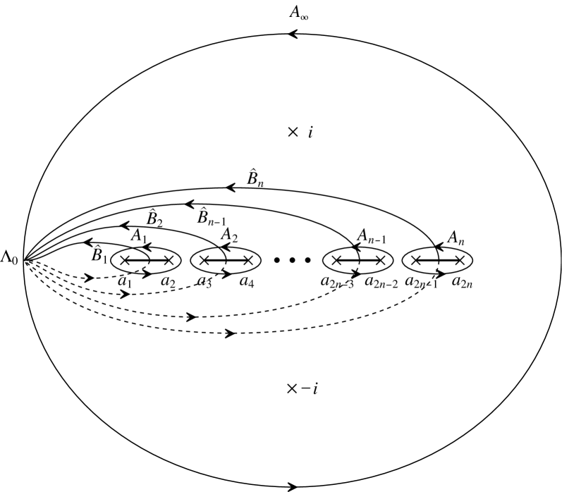
Figure 1: The contours. Those on the second sheet are shown in broken lines.

$y(z)$ is given by the equation

$$y(z) = W^{\prime}(z)-2\mu\omega(z)$$ (3.12)

$$= -\frac{\sqrt{\prod_{k=1}^{2n}(z-a_{k})}}{2\pi i}\left(\oint_{A_{\infty}}-\oint_{x=i}-\oint_{x=-i}\right)dx\frac{W^{\prime}(x)}{(z-x)\sqrt{\prod_{k=1}^{2n}(x-a_{k})}},$$

so that

$$\oint_{A_{j}}dzy(z)~{}=~{}-4\pi i\mu_{j}~{}~{}(j=1,\ldots,n).$$ (3.13)

Our aim is to express $\frac{\partial F_{0}}{\partial\mu_{j}}$ in terms of the periods of $y(z)dz$. For this purpose we need to compute $\frac{\partial y(z)}{\partial\mu_{j}}dz$, which may be found by simply studying the locations of the singularities, as was done in [23]. In the present case, however, $W^{\prime}(z)$ has extra pole singularities at $z=\pm i$ with residue $\mu$ coming from the unitary Haar measure and must be also taken into account.

$y(z)dz$ has the following properties:

• Since the contours of (3.12) do not enclose $x=z$, the integrals give single-valued functions of $z$ on the complex plane. Therefore $y(z)$ reverses its sign under the exchange of the first and second sheets.

• Since we have assumed that $W_{U}(U)$ is a polynomial of $U$ and $U^{-1}$, $y(z)dz$ is regular at $z=\infty,\tilde{\infty}$, where we denote here and henceforth a point on the second sheet by its value of $z$ with tilde.

• Since $\omega(z)dz$ must be regular at $z=\pm i$ on the first sheet, $y(z)dz$ exhibits the same singular behavior as $W^{\prime}(z)dz$ at $z=\pm i$, and as $-W^{\prime}(z)dz$ at $z=\widetilde{\pm i}$.

These properties, together with the condition (3.13), uniquely determine the $\mu_{j}$ derivative of $y(z)dz$ as

$$\frac{\partial y(z)}{\partial\mu_{j}}dz~{}=~{}-4\pi i~{}\hat{\omega}_{j}(z),$$ (3.14)

where

$$\hat{\omega}_{j} = \omega_{j}+\hat{\omega}_{n}~{}~{}~{}(j=1,\ldots,n-1),$$

$$\hat{\omega}_{n} = -\frac{1}{4\pi i}\left(\omega_{(+i)-\widetilde{(+i)}}+\omega_{(-i)-\widetilde{(-i)}}\right).$$ (3.15)

$\omega_{j}$’s are holomorphic differentials normalized as

$$\oint_{A_{i}}\omega_{j} = \delta_{ij}~{}~{}~{}(j=1,\ldots,n-1),$$ (3.16)

and $\omega_{a-b}(z)$ denotes a zero A-period abelian differential of the third kind having simple poles at $z=a,b$ with residue $\pm 1$, respectively.

Having computed $\frac{\partial y(z)}{\partial\mu_{j}}dz$, we are now able to derive the special geometry relation. Differentiating the free energy $F_{0}$ by $\mu_{j}$, we have.

$$\frac{\partial F_{0}}{\partial\mu_{i}} = -\frac{1}{2}\sum_{j=1}^{n}\oint_{A_{j}}\hat{\omega}_{i}(z)W(z)+\frac{1}{8\pi i}\sum_{j=1}^{n}\oint_{A_{j}}dzy(z)\log(z^{2}+1)$$ (3.17)

$$+\lim_{\Lambda_{0}\rightarrow-\infty}\left[-\pi i\sum_{j=1}^{n}\mu_{j}\int_{\hat{B}_{j}}\omega_{i}(z)~{}+\frac{1}{4}\int_{\hat{B}_{i}}dzy(z)~{}-\frac{1}{2}W(\Lambda_{0})\right.$$

$$\left.-\frac{\mu}{2}\log(\Lambda_{0}^{2}+1)~{}+2\mu\log|\Lambda_{0}|\right]$$

$$= -\frac{1}{2}\sum_{j=1}^{n}\oint_{A_{j}}\hat{\omega}_{i}(z)W(z)~{}+\lim_{\Lambda_{0}\rightarrow-\infty}\left[-\pi i\sum_{j=1}^{n}\mu_{j}\int_{\hat{B}_{j}}\omega_{i}(z)\right.$$

$$\left.+\lim_{\epsilon\rightarrow 0}\left(\frac{1}{4}\left(\int_{\hat{B}_{i}}\!\!\!+\int_{\Lambda_{0}}^{i-\epsilon}\!\!\!+\int_{\Lambda_{0}}^{-i-\epsilon}\right)dzy(z)~{}-W(i-\epsilon)-W(-i-\epsilon)\right)\rule{0.0pt}{19.91692pt}\right].$$

This expression can be simplified because one can show that the following relation holds:

$$-\frac{1}{2}\sum_{j=1}^{n}\oint_{A_{j}}\hat{\omega}_{i}(z)W(z)~{}+\lim_{\Lambda_{0}\rightarrow-\infty}\left[-\pi i\sum_{j=1}^{n}\mu_{j}\int_{\hat{B}_{j}}\omega_{i}(z)\right]$$ (3.18)

$$= \lim_{\Lambda_{0}\rightarrow-\infty}\left[\frac{1}{4}\lim_{\epsilon\rightarrow 0}\left(\int_{\hat{B}_{i}}\!\!\!+\int_{\Lambda_{0}}^{i-\epsilon}\!\!\!+\int_{\Lambda_{0}}^{-i-\epsilon}\right)dzy(z)~{}-W(i-\epsilon)-W(-i-\epsilon)\right].$$

This relation may be derived in the way parallel to that in [23] by using Riemann’s bilinear relation; we give a brief sketch of it in Appendix B. Thus we obtain the final result

$$\displaystyle\hskip-48.0pt\frac{\partial F_{0}}{\partial\mu_{i}} = \frac{1}{2}\lim_{\epsilon\rightarrow 0}\left[\lim_{\Lambda_{0}\rightarrow-\infty}\left(\int_{\hat{B}_{i}}\!\!\!+\int_{\Lambda_{0}}^{i-\epsilon}\!\!\!+\int_{\Lambda_{0}}^{-i-\epsilon}\right)dzy(z)~{}-W(i-\epsilon)-W(-i-\epsilon)\right]$$ (3.19)

$$= \frac{1}{2}\lim_{\epsilon\rightarrow 0}\left[\int_{\widetilde{-i+i\epsilon}}^{i-i\epsilon}\!\!\!\!\!\!\!\!\!\mbox{\scriptsize($i$th cut) }dzy(z)~{}-W(i-i\epsilon)-W(\widetilde{-i+i\epsilon})\right],$$

where in the last line the integration contour passes through the $i$th cut. If we go back to the $w$-plane (2.6), the contour runs from a point infinitely close to $w=0$ to another to $w=\infty$.

4 Application I : $N=2$ Gauge Theory via Unitary Matrix Models

It is now well-known that the effective superpotential and other F-terms in ${\cal N}=1$ supersymmetric gauge theory can be calculated using hermitian matrix models [4, 5]. The ${\cal N}=2$ limit may also be achieved by turning off the superpotential with the effective superpotential kept extremized with respect to the glueball fields [34]. On the other hand, it has been shown [5] that there is another route to realize more directly the pure $SU(2)$ Seiberg-Witten curve via a unitary matrix model without referring to any ${\cal N}=1$ theory. In this section we will apply the duality transformation to this unitary matrix model to examine whether the genus-1 topological amplitude, obtained by other means, is correctly reproduced in this framework.

4.1 2-cut Solutions of The Gross-Witten Model

To realize the pure $SU(2)$ Seiberg-Witten curve we again consider the Gross-Witten model, though this time focus on 2-cut solutions. In this case it is convenient to shift $\theta$ by 90 degrees in (2.16) and consider the potential

$$W_{U}(e^{i\theta}) = -2\sin\theta,$$ (4.1)

$$W(z) = \frac{4z}{1+z^{2}}+\mu\log(1+z^{2}).$$ (4.2)

We let $a_{1}<\cdots<a_{4}$ be the end points of the cuts; they are constrained by

$$\left(\oint_{A_{1}}+\oint_{A_{2}}\right)dx\frac{W^{\prime}(x)}{\sqrt{\prod_{k=1}^{4}(x-a_{k})}} = 0,$$

$$\left(\oint_{A_{1}}+\oint_{A_{2}}\right)dx\frac{xW^{\prime}(x)}{\sqrt{\prod_{k=1}^{4}(x-a_{k})}} = 0,$$ (4.3)

$$\left(\oint_{A_{1}}+\oint_{A_{2}}\right)dx\frac{x^{2}W^{\prime}(x)}{\sqrt{\prod_{k=1}^{4}(x-a_{k})}} = 4\pi i\mu.$$

One can straightforwardly compute the differential $y(z)dz$ to find

$$y(z) = -\frac{\sqrt{\prod_{k=1}^{4}(z-a_{k})}}{2\pi i}\left(\oint_{A_{\infty}}-\oint_{x=i}-\oint_{x=-i}\right)dx\frac{W^{\prime}(x)}{(z-x)\sqrt{\prod_{k=1}^{4}(x-a_{k})}}$$ (4.4)

$$= \frac{8}{c}\frac{\sqrt{\prod_{k=1}^{4}(z-a_{k})}}{(z^{2}+1)^{2}},$$

where we put $\sqrt{\prod_{k=1}^{4}(i-a_{k})}=\sqrt{\prod_{k=1}^{4}(-i-a_{k})}\equiv c$.

To incorporate the end-point conditions (4.3) we go back to the $w$-plane (2.6). The two cuts are mapped to two arcs located on the unit circle with end points given by

$$T_{k}=\frac{i-a_{k}}{i+a_{k}}~{}~{}~{}(k=1,\ldots,4).$$ (4.5)

Then the conditions (4.3) are fulfilled if and only if $T_{k}$’s are the roots of the following equation of $U$:

$$U^{4}-2i\mu U^{3}+\sigma_{2}U^{2}+2i\mu U+1=0,$$ (4.6)

where

$$\sigma_{2}\equiv T_{1}T_{2}+T_{1}T_{3}+T_{1}T_{4}+T_{2}T_{3}+T_{2}T_{4}+T_{3}T_{4}$$ (4.7)

is a free parameter, which is eventually identified as (essentially) the $u$ modulus of the Seiberg-Witten curve. Using the relations between the roots and the coefficients, $y(z)$ (4.4) may be written in the form obtained in [5]:

$$y(z)dz=2\sqrt{\cos^{2}\theta+\mu(\sin\theta-u)}~{}d\theta$$ (4.8)

with $u\equiv\frac{2-\sigma_{2}}{4\mu}$. The ${\cal N}=2$ curve and differential are obtained by restricting the moduli to a co-dimension one sublocus in the following way: We first scale $y(z)dz$ as

$$y(z)dz \equiv 2\sqrt{\mu}~{}y_{\mbox{\scriptsize SW}}(\theta)d\theta$$ (4.9)

and take the $\mu\rightarrow\infty$ limit. Then we obtain the Seiberg-Witten curve for the pure $SU(2)$ gauge theory:

$$y_{\mbox{\scriptsize SW}}^{2}-\sin\theta+u = 0.$$ (4.10)

On the other hand, we choose, as was done in [34], $\mu_{1}$ and $\mu(=\mu_{1}+\mu_{2})$ (instead of $\mu_{1}$ and $\mu_{2}$) as independent parameters. Using the special geometry relation in the previous section, we have

$$\left.\frac{\partial F_{0}}{\partial\mu_{1}}\right|_{\mbox{\scriptsize$\mu$}} = \left.\frac{\partial F_{0}}{\partial\mu_{1}}\right|_{\mbox{\scriptsize$\mu_{2}$}}-\left.\frac{\partial F_{0}}{\partial\mu_{2}}\right|_{\mbox{\scriptsize$\mu_{1}$}}$$ (4.11)

$$= -\frac{1}{2}\oint_{B}dzy(z),$$

where $B=\hat{B}_{2}\hat{B}_{1}^{-1}$. Therefore $y_{\mbox{\scriptsize SW}}(\theta)d\theta$ is indeed a Seiberg-Witten differential.

4.2 Gravitational $F$-terms via The Unitary Matrix Model

We are now interested in the genus-1 free energy of this matrix model. In the 2-cut case it is given by [13]

$$F_{1}=-\frac{1}{24}\log\prod_{j=1}^{4}M_{j}-\frac{1}{2}\log|K(k)|-\frac{1}{12}\log\prod_{i<j}(a_{i}-a_{j})^{2}+\frac{1}{4}\log(|a_{1}-a_{3}||a_{2}-a_{4}|),$$ (4.12)

where the moments are defined by

$$M_{i} = \frac{1}{2\pi i}\left(\oint_{A_{1}}\!\!\!+\oint_{A_{2}}\right)dx\frac{\frac{1}{\mu}W^{\prime}(x)}{(x-a_{i})\sqrt{\prod_{k=1}^{4}(x-a_{k})}},$$ (4.13)

and

$$K(k)=\int_{0}^{1}dt\frac{1}{\sqrt{(1-t^{2})(1-k^{2}t^{2})}}$$ (4.14)

is the complete elliptic integral of the first kind with modulus

$$k^{2}~{}=~{}\frac{(a_{1}-a_{4})(a_{2}-a_{3})}{(a_{1}-a_{3})(a_{2}-a_{4})}~{}=~{}\frac{2\sqrt{u^{2}-1}}{u+\sqrt{u^{2}-1}}.$$ (4.15)

Here we note that $y_{SW}^{2}$ (4.10) has at most only two zeros on the unit circle, and hence is only defined as an analytic continuation of the 2-cut solutions. Therefore we evaluate $M_{i}$’s where it is well-defined, and then take the $\mu\rightarrow\infty$ limit afterwards. This is very different from the situation in the hermitian matrix realization [35] where a spectral curve “really” exists in the ${\cal N}=2$ limit. Nevertheless, despite the difference, $F_{1}$ (4.12) obtained as an analytic continuation correctly reproduces the known result, as we will see below.

$M_{1}$ is found after some straightforward residue computations as

$$M_{1} = -\frac{2}{\mu c^{3}(a_{1}^{2}+1)}\left[\rule{0.0pt}{11.38109pt}-8+6(a_{2}a_{3}+a_{2}a_{4}+a_{3}a_{4})-3a_{1}(a_{2}+a_{3}+a_{4}-a_{2}a_{3}a_{4})\right.$$ (4.16)

$$\left.\hskip 42.67912pt+a_{1}^{2}(-5+3(a_{2}a_{3}+a_{2}a_{4}+a_{3}a_{4}))\right]-\frac{2(-\mu a_{1}+2)}{\mu c(a_{1}^{2}+1)}$$

with $c^{2}=\frac{16}{\sigma_{2}+2}$. Various symmetric polynomials of $a_{i}$’s turn out to be

$$a_{1}+a_{2}+a_{3}+a_{4} = \frac{2\mu}{\mu u-1},$$

$$a_{1}a_{2}+a_{1}a_{3}+a_{1}a_{4}+a_{2}a_{3}+a_{2}a_{4}+a_{3}a_{4} = 2+\frac{4}{\mu u-1},$$

$$a_{1}a_{2}a_{3}+a_{1}a_{2}a_{4}+a_{1}a_{3}a_{4}+a_{2}a_{3}a_{4} = \frac{2\mu}{\mu u-1},$$

$$a_{1}a_{2}a_{3}a_{4} = 1.\rule{0.0pt}{14.22636pt}$$ (4.17)

Thus we find

$$\prod_{j=1}^{4}M_{j}=\frac{(1-\mu u)^{6}}{\mu^{4}}~{}=~{}\mu^{2}u^{6}\left(1+{\cal O}(\mu^{-1})\right).$$ (4.18)

The discriminant can be computed as

$$\prod_{i<j}(a_{i}-a_{j})^{2} = \frac{16^{2}\mu^{2}(\mu^{2}-4\mu u+4)^{2}(u^{2}-1)}{(\mu u-1)^{6}}$$ (4.19)

$$\stackrel{{\scriptstyle\mu\rightarrow\infty}}{{\longrightarrow}} \frac{16^{2}(u^{2}-1)}{u^{6}},$$

and also

$$|a_{1}-a_{3}||a_{2}-a_{4}| = 2\left(1+\sqrt{1-\frac{1}{u^{2}}}\right).$$ (4.20)

Plugging these data into (4.12), we see that the $\log u$ terms precisely cancel. This leaves

$$F_{1} = -\frac{1}{2}\log K(k)-\frac{1}{12}\log(u^{2}-1)+\frac{1}{4}\log(u+\sqrt{u^{2}-1})-\frac{1}{12}\log 2\mu+{\cal O}(\mu^{-1}),$$

the $u$-dependent part of which is in agreement with the known genus-1 result [36, 35].

5 Application II : A Matrix Model Mirror of A Chern-Simons Theory

5.1 The Transformation

The final example we consider is a matrix model mirror of a Chern-Simons theory. It has been proposed [8] that the partition function of the $SU(N)$ Chern-Simons theory of $S^{3}$ is equal to the partition function of a matrix model with a “Wick-rotated” Jacobian as

$$Z_{\mbox{\scriptsize CS}} = e^{-\frac{\mu}{12}(N^{2}-1)}Z,$$

$$Z = \int\prod_{j=1}^{N}du_{j}e^{-\frac{1}{g_{s}}\frac{u_{j}^{2}}{2}}\prod_{k<l}^{N}\sinh^{2}\frac{u_{k}-u_{l}}{2}.$$ (5.1)

In this section we apply the duality transformation to this model, compute the genus-0 and -1 free energies and confirm that they indeed reproduce those of the Chern-Simons theory. In fact, it was already proven by Tierz [28] that the partition function (5.1) is equal to the Chern-Simons partition function to all orders in the $1/N$ expansion, by utilizing yet another transformation (as in footnote 4) to map (5.1) to that of a hermitian matrix model (different from ours) and use its orthogonal polynomials. However, there are still some benefits in considering our transformation in this model as follows: First, it will also demonstrate how to compute explicitly the lower genus free energies in other such models that have the same measure of the “Wick-rotated” type, such as those proposed to be related to some five-dimensional gauge theories [10], even where no good orthogonal polynomials are available. Secondly, because our transformation induces no singularity near the origin in the potential, one can show the special geometry relation in these models by only slightly modifying the proof for hermitian models. Finally, for the same reason, the relation to the KP hierarchy is made manifest by our transformation, and not by the one adopted in [28] because of its $\log$ branch at the origin.

For the measure of the type (5.1) the transformation we need is

$$\lambda_{j} = \tanh\frac{u_{j}}{2}.$$ (5.2)

$Z$ (5.1) can then be written as

$$Z~{}=~{}2^{N}\int\prod_{j=1}^{N}d\lambda_{j}e^{-\frac{N}{\mu}\left[\frac{1}{2}\left(\log\frac{1+\lambda_{j}}{1-\lambda_{j}}\right)^{2}+\mu\log(1-\lambda_{j}^{2})\right]}\prod_{k<l}^{N}(\lambda_{k}-\lambda_{l})^{2}.$$ (5.3)

Comparing it with (2.13), we find that the Chern-Simons matrix model has, up to an $N$-independent multiplicative constant, the same partition function as that of the hermitian matrix model with a potential

$$W(z)=\frac{1}{2}\left(\log\frac{1+z}{1-z}\right)^{2}+\mu\log(1-z^{2}),$$ (5.4)

or as that of the hermitian matrix model coupled to $N_{f}=2N$ vectors having real masses $\pm 1$ with a potential

$$W_{\Phi}(z)=\frac{1}{2}\left(\log\frac{1+z}{1-z}\right)^{2}.$$ (5.5)

In this case, therefore, the potential of the resulting dual hermitian matrix model has branch cuts of $\log$ ending on the real axis; this is not a problem because the eigenvalues are located only on the interval between 1 and $-1$, as is clear from the transformation (5.2).

5.2 The Spectral Curve

We will now rederive the (nontrivial part of the) geometry of the deformed conifold as the spectral curve, following the standard procedure as before. Let us consider a 1-cut solution with a cut $[a,b]$. The end point conditions (2.19) with $W$ (5.4) imply

$$b=-a=\sqrt{1-e^{-\mu}}~{}~{}~{}(>0).$$ (5.6)

The resolvent is also given by (2.18) with $W$ (5.4). The contribution of the second term of $W$ is simply obtained by residue computations, while the contribution of the first term can be written as

$$\frac{(z^{2}-b^{2})^{\frac{1}{2}}}{4\pi i\mu}(I(z)+I(-z)),$$ (5.7)

where

$$I(z) \equiv \oint_{A}dx\frac{2\log(1+x)}{(z-x)(1-x^{2})(x^{2}-b^{2})^{\frac{1}{2}}}.$$ (5.8)

If the contour $A$ is deformed to a large circle around infinity, $I(z)$ also picks up the contribution from the difference of the integrals along both sides of the branch cut of $\log(1+x)$. After some calculations we find

$$I(z) = \frac{4\pi i}{(1-z^{2})\sqrt{z^{2}-b^{2}}}\log\frac{z+b^{2}+\sqrt{(z^{2}-b^{2})(1-b^{2})}}{z+\sqrt{z^{2}-b^{2}}}$$ (5.9)

$$+\frac{2\pi i}{\sqrt{1-b^{2}}}\left(\frac{\log(1+\sqrt{1-b^{2}})}{1-z}-\frac{1}{1+z}\log\frac{1+\sqrt{1-b^{2}}}{2(1-b^{2})}-\frac{\log 2}{1-z}\right),$$

and

$$\omega(z) = \frac{1}{\mu(1-z^{2})}\left[\log\frac{z^{2}+b^{2}+\sqrt{(z^{2}-b^{2})(1-b^{2})}}{z^{2}-b^{2}+\sqrt{(z^{2}-b^{2})(1-b^{2})}}\right.$$ (5.10)

$$\left.+\sqrt{\frac{z^{2}-b^{2}}{1-b^{2}}}\log(1-b^{2})-\mu\left(z-\sqrt{\frac{z^{2}-b^{2}}{1-b^{2}}}\right)\right].$$

Since

$$\mu=-\log(1-b^{2}),$$ (5.11)

$y(z)$ is simply given by

$$y(z) = W^{\prime}(z)-2\mu\omega(z)$$ (5.12)

$$= -\frac{2}{1-z^{2}}\left(\log\frac{-\sqrt{z^{2}-b^{2}}+\sqrt{1-b^{2}}}{\sqrt{z^{2}-b^{2}}+\sqrt{1-b^{2}}}\right).$$

Going back to the original $u$ plane by the relation

$$z = \tanh\frac{u}{2}~{}=~{}\frac{e^{u}-1}{e^{u}+1},$$ (5.13)

the differential $y(z)dz$ becomes

$$y(z)dz = 2du\left(\log\frac{1+e^{-u}+\sqrt{(1+e^{-u})^{2}-4e^{\mu-u}}}{2}+\frac{u-\mu}{2}\right).$$ (5.14)

Thus one recovers the equation given in [9] describing the mirror of a resolved conifold [37], which can be made identical to the equation of a deformed conifold by a change of variables.

5.3 The Special Geometry Relation and Free Energies

The special geometry relation for this matrix model can be similarly obtained, although the branch cuts of $W^{\prime}(z)$, which run from $-1$ to $-\infty$ and from $+1$ to $+\infty$, add an extra complication; one must specify the relative location of the branch cut of $\log|\lambda|$ (taking $\lambda_{01}\equiv 0$) in (3.9) and define the contour $\hat{B}_{1}$ accordingly. Then one differentiates $F_{0}$ by $\mu$ and employ an identity similarly derived by using Riemann’s bilinear relation. Although tedious, the calculation can be done similarly as before and we only describe the result:

$$\frac{\partial F_{0}}{\partial\mu} = \lim_{\epsilon\rightarrow 0}\left[\int_{b}^{1-\epsilon}dzy(z)-W(1-\epsilon)\right],$$ (5.15)

$$\frac{\partial y(z)}{\partial\mu}dz = \omega_{1-\widetilde{1}}(z)+\omega_{(-1)-\widetilde{(-1)}}(z),$$ (5.16)

where, as before, $\omega_{1-\widetilde{1}}(z)$ ($\omega_{(-1)-\widetilde{(-1)}}(z)$) is a zero A-period abelian differential of the third kind having two simple poles, one at $z=1$ ($z=-1$) with residue $1$ and the other at $z=\widetilde{1}$ ($z=\widetilde{-1}$) with residue $-1$. Differentiating (5.15) by $\mu$ again and using (5.16), we find

$$\frac{\partial^{2}F_{0}}{\partial\mu^{2}} = \lim_{\epsilon\rightarrow 0}\left[\int_{b}^{1-\epsilon}dz\sqrt{\frac{1-b^{2}}{z^{2}-b^{2}}}\left(\frac{1}{z-1}-\frac{1}{z+1}\right)-\log 2\epsilon\right]$$ (5.17)

$$= \log\frac{b^{2}}{4(1-b^{2})}.$$

Integrating over $\mu$ yields

$$F_{0} = -\sum_{n=1}^{\infty}\frac{e^{-n\mu}}{n^{3}}+\frac{\mu^{3}}{6}-\frac{\mu^{2}}{2}\log 4+\mbox{const}\times\mu~{}+\mbox{const}.$$ (5.18)

$F_{0\mbox{\scriptsize CS}}=F_{0}-\frac{\mu^{3}}{12}$ agrees with the known result [38, 39].

The genus-1 free energy may also be computed by the formula of Ambjørn et. al. [12] again:

$$F_{1} = -\frac{1}{24}(\log M_{1}+\log J_{1}+4\log 2b).$$ (5.19)

After some calculations we find

$$M_{1}~{}=~{}J_{1} = \frac{4}{\mu\sqrt{1-b^{2}}^{3}},$$ (5.20)

and hence obtain

$$F_{1} = -\frac{1}{12}\left(\frac{3}{2}\mu-\log\mu+\log(1-e^{-\mu})+4\log 2\right),$$ (5.21)

which correctly reproduces the known genus-1 Chern-Simons free energy $F_{1\mbox{\scriptsize CS}}=F_{1}+\frac{\mu}{12}$ including the $\log\mu$ term [38, 39].

6 Conclusions

In this paper we have shown that a hermitian 1-matrix model with the potential $W(\Phi)$ and a unitary 1-matrix model with the potential $W_{U}(U)$ are nothing but different descriptions of the same model if they are related with each other by the equation (2.12). The extra logarithmic term on the hermitian side has been further interpreted as an effect of the coupling to $2N$ vectors. This duality is particularly useful to compute lower genus free energies in unitary as well as other matrix models with the unitary matrix Haar measure, and we have demonstrated the use of it in various examples. It allowed us not only to rederive the known facts by simply using the familiar hermitian matrix model technologies, but also to establish some new results on matrix models and gauge theory. We have shown that the unitary matrix formulation of the ${\cal N}=2$ pure $SU(2)$ gauge theory correctly reproduces the genus-1 amplitude, and also given the rigorous forms of the special geometry relations in unitary as well as the Chern-Simons matrix models.

This duality is not only of practical but also of conceptual importance; it has revealed that unitary and hermitian 1-matrix models have no essential difference and can be mapped to each other via the transformation (2.12). An immediate consequence of this fact is that the partition function of a unitary 1-matrix model is also a $\tau$ function of the KP hierarchy. It also provides an explanation of why the critical behaviors of both unitary and (even-potential) hermitian 1-matrix models are described by the same (Painlevé II) equation when two clusters of eigenvalues join: this is accounted for by the universality with respect to even perturbations (e.g. [40]) in hermitian 1-matrix models.

It is amusing that while the topological B-model on a deformed conifold is known to be equivalent to $c=1$ strings at the self-dual radius [41] and realized as the Penner model [42], the hermitian matrix model obtained after applying the duality to the Chern-Simons matrix model may be regarded as a “two-flavor” extension of the (generalized) Penner model.

It would be interesting to apply this duality to the matrix models proposed to describe some five-dimensional gauge theories and compare the lower genus amplitudes with Nekrasov’s formula [43].

Appendix A  The Multi-cut Free Energy

In this Appendix we give a derivation of the formula (3.9) for the genus-0 multi-cut free energy in hermitian 1-matrix models. We start from the well-known expression [32]

$$\frac{F_{0}}{\mu^{2}} = -\frac{1}{\mu}\int_{-\infty}^{\infty}d\lambda\rho(\lambda)W(\lambda)+\int_{-\infty}^{\infty}d\lambda\int_{-\infty}^{\infty}d\lambda^{\prime}\rho(\lambda)\rho(\lambda^{\prime})\log|\lambda-\lambda^{\prime}|,$$ (A.1)

which is valid for any number of the cuts $n$. It is convenient to define

$$\sigma(\lambda) \equiv \int_{-\infty}^{\lambda}d\lambda^{\prime}\rho(\lambda^{\prime}).$$ (A.2)

Due to (3.10) we have

$$\sigma(a_{1}) = 0,$$

$$\sigma(a_{2}) = \sigma(a_{3})~{}=~{}\frac{\mu_{1}}{\mu},$$

$$\cdots,$$

$$\sigma(a_{2j}) = \sigma(a_{2j+1})~{}=~{}\sum_{k=1}^{j}\frac{\mu_{k}}{\mu},$$

$$\cdots,$$

$$\sigma(a_{2n}) = 1.$$ (A.3)

Using $\sigma(\lambda)$, the second term of (A.1) can be integrated by parts to give

The second term $$= \int_{-\infty}^{\infty}d\lambda\rho(\lambda)\sum_{j=1}^{n}\int_{a_{2j-1}}^{a_{2j}}d\lambda^{\prime}\rho(\lambda^{\prime})\log|\lambda-\lambda^{\prime}|$$ (A.4)

$$= \int_{-\infty}^{\infty}d\lambda\rho(\lambda)\sum_{j=1}^{n}\left(\left[\rule{0.0pt}{14.22636pt}\sigma(\lambda^{\prime})\log|\lambda-\lambda^{\prime}|\right]_{a_{2j-1}}^{a_{2j}}+\int_{a_{2j-1}}^{a_{2j}}d\lambda^{\prime}\frac{\sigma(\lambda^{\prime})}{\lambda-\lambda^{\prime}}\right)$$

$$= \int_{-\infty}^{\infty}d\lambda\rho(\lambda)\sum_{j=1}^{n}\left(\frac{1}{\mu}\sum_{k=1}^{j}\mu_{k}\log|\lambda-a_{2j}|-\frac{1}{\mu}\sum_{k=1}^{j-1}\mu_{k}\log|\lambda-a_{2j-1}|\right)$$

$$-\sum_{j=1}^{n}\int_{a_{2j-1}}^{a_{2j}}d\lambda\sigma(\lambda)\frac{1}{2\mu}W^{\prime}(\lambda),$$

where in the last line we have used the large $N$ saddle point equation

$$-\frac{1}{\mu}W^{\prime}(\lambda)+2\int_{-\infty}^{\infty}\frac{\rho(\lambda^{\prime})}{\lambda-\lambda^{\prime}} = 0.$$ (A.5)

The last term is integrated by parts again to yield

$$-\sum_{j=1}^{n}\int_{a_{2j-1}}^{a_{2j}}d\lambda\sigma(\lambda)\frac{1}{2\mu}W^{\prime}(\lambda) = \frac{1}{2\mu}\int_{-\infty}^{\infty}d\lambda\rho(\lambda)V(\lambda)-\frac{1}{2\mu}\left(\frac{\mu_{1}}{\mu}(W(a_{2})-W(a_{3}))+\cdots\right.$$ (A.6)

$$\left.~{}~{}~{}~{}~{}~{}+\frac{\sum_{k=1}^{n-1}\mu_{k}}{\mu}(W(a_{2n-2})-W(a_{2n-1}))+W(a_{2n})\right).$$

Therefore we get

$$\frac{F_{0}}{\mu^{2}} = -\frac{1}{2\mu}\int_{-\infty}^{\infty}d\lambda\rho(\lambda)W(\lambda)$$ (A.7)

$$+\frac{\mu_{1}}{\mu}\left(-\frac{1}{2\mu}(W(a_{2})-W(a_{3}))+\int_{-\infty}^{\infty}\rho(\lambda)\log\left|\frac{\lambda-a_{2}}{\lambda-a_{3}}\right|\right)$$

$$+\cdots$$

$$+\frac{\sum_{k=1}^{j}\mu_{k}}{\mu}\left(-\frac{1}{2\mu}(W(a_{2j})-W(a_{2j+1}))+\int_{-\infty}^{\infty}\rho(\lambda)\log\left|\frac{\lambda-a_{2j}}{\lambda-a_{2j+1}}\right|\right)$$

$$+\cdots$$

$$+\left(-\frac{1}{2\mu}W(a_{2n})+\int_{-\infty}^{\infty}\rho(\lambda)\log\left|\lambda-a_{2n}\right|\right).$$

Here the saddle point equation (A.5) can be used to replace $a_{2k-1}$, $a_{2k}$ with an arbitrary $\lambda_{0k}$ on the $k$th cut, for all $k=1,\ldots,n$. With this replacement we end up with the formula (3.9).

Appendix B  A Derivation of Eq.(3.18)

Let $\Sigma$ be a hyper-elliptic Riemann surface defined by

$$Y^{2} = \prod_{k=1}^{2n}(z-a_{k}).$$ (B.1)

The first step in using Riemann’s bilinear relation is to cut out $\Sigma$ along the cycle

$$A_{n-1}B_{n-1}A_{n-1}^{-1}B_{n-1}^{-1}\cdots A_{1}B_{1}A_{1}^{-1}B_{1}^{-1}~{}\hat{B}_{n}P_{-}^{-1}A_{\infty}P_{+}^{-1}\hat{B}_{n}^{-1}P_{\tilde{-}}^{-1}A_{\tilde{\infty}}P_{\tilde{+}}^{-1}$$ (B.2)

to get a simply-connected polygonal region, which we denote by $\Sigma^{\prime}$. For the definitions of the cycles see Figures 1 and 2.

Figure 2: More definitions of the contours. The bold lines from $\pm i$ to $\Lambda_{0}$ denote the branch cut of $\log(z\mp i)$. $A_{\tilde{\infty}}$, $P_{\tilde{\pm}}^{-1}$ are the same as those without tildes but lying on the second sheet.

Next we consider

$$\Omega_{i}(z) \equiv \int_{z_{0}}^{z}\omega_{i}~{}~{}~{}(i=1,\ldots,n-1)$$ (B.3)

for some reference point $z_{0}$ on $\Sigma^{\prime}$, then $\Omega_{i}(z)$’s are single-valued, everywhere holomorphic functions inside $\Sigma^{\prime}$. Then for each $i$ Riemann’s bilinear relation can be obtained by computing

$$\int_{\partial\Sigma^{\prime}}dzy(z)\Omega_{i}(z)$$ (B.4)

in two ways, by the residue computation inside $\Sigma^{\prime}$, and by evaluating the integral along the boundary of $\Sigma^{\prime}$. The total residue is trivially zero. On the other hand, one can evaluate the integral on the edges pairwise as

$$\left(\oint_{A_{j}}+\oint_{A_{j}^{-1}}\right)dzy(z)\Omega_{i}(z) = 4\pi i\mu_{j}\oint_{B_{j}}\omega_{i},$$

$$\left(\oint_{B_{j}}+\oint_{B_{j}^{-1}}\right)dzy(z)\Omega_{i}(z) = \delta_{ij}\oint_{B_{j}}y(z),$$

$$\left(\int_{\hat{B}_{n}}+\int_{\hat{B}_{n}^{-1}}\right)dzy(z)\Omega_{i}(z) = 0,$$

$$\lim_{\Lambda_{0}\rightarrow-\infty}\left(\int_{\hat{P}_{-}^{-1}}+\int_{\hat{P}_{+}^{-1}}\right)dzy(z)\Omega_{i}(z) = -\sum_{j=1}^{n}\oint_{A_{j}}W(z)\omega_{i}(z)-4\pi i\mu\Omega_{i}(-\infty),$$

$$\lim_{\Lambda_{0}\rightarrow-\infty}\left(\int_{\hat{P}_{\tilde{-}}^{-1}}+\int_{\hat{P}_{\tilde{+}}^{-1}}\right)dzy(z)\Omega_{i}(z) = -\sum_{j=1}^{n}\oint_{A_{j}}W(z)\omega_{i}(z)+4\pi i\mu\Omega_{i}(\widetilde{-\infty}),$$ (B.5)

and

$$\oint_{A_{\infty}}dzy(z)\Omega_{i}(z) = \oint_{A_{\tilde{\infty}}}dzy(z)\Omega_{i}(z)~{}=~{}0.$$ (B.6)

Stokes’ theorem implies that the sum of all these integrals is zero. Noting that

$$\Omega_{i}(\infty)-\Omega_{i}(\widetilde{-\infty}) = \lim_{\Lambda_{0}\rightarrow-\infty}\int_{\hat{B}_{n}}\omega_{i},$$ (B.7)

we have

$$-4\pi i\sum_{j=1}^{n}\mu_{j}\lim_{\Lambda_{0}\rightarrow-\infty}\int_{\hat{B}_{j}}\omega_{i}+\oint_{B_{i}}dzy(z)-2\sum_{j=1}^{n}\oint_{A_{j}}W(z)\omega_{i}(z) = 0$$ (B.8)

for $i=1,\ldots,n-1$.

To derive a relation involving the period of $\hat{\omega}_{n}$ we also consider

$$\int_{\partial\Sigma^{\prime}}dzy(z)\Omega_{n}(z),$$ (B.9)

where

$$\Omega_{n}(z) \equiv \int_{z_{0}}^{z}\hat{\omega}_{n}$$ (B.10)

is also a single-valued holomorphic function inside $\Sigma^{\prime}$. Taking special care about the singular behavior of $y(z)\Omega_{n}(z)$ near $z=\pm i$, one may similarly compute (B.9) in two ways to obtain

$$\hskip-28.45274pt-\frac{1}{2}\sum_{j=1}^{n}\oint_{A_{j}}W(z)\hat{\omega}_{n}(z)+\lim_{\Lambda_{0}\rightarrow-\infty}\left(-\pi i\sum_{j=1}^{n}\mu_{j}\int_{\hat{B}_{j}}\hat{\omega}_{n}\right)$$

$$=\lim_{\Lambda_{0}\rightarrow-\infty}\left[\frac{1}{4}\int_{\hat{B}_{n}}dzy(z)\right.$$

$$\left.\hskip 51.21495pt+\frac{1}{8\pi i}\left(\int_{P_{-}^{-1}}\!\!\!+\int_{P_{+}^{-1}}\right)dz(y(z)-W^{\prime}(z))\log(z^{2}+1)-\frac{1}{2}W(\Lambda_{0})\right].$$ (B.11)

One can then use (B.8) in this equation to see also that

$$\hskip-28.45274pt-\frac{1}{2}\sum_{j=1}^{n}\oint_{A_{j}}W(z)\hat{\omega}_{i}(z)+\lim_{\Lambda_{0}\rightarrow-\infty}\left(-\pi i\sum_{j=1}^{n}\mu_{j}\int_{\hat{B}_{j}}\hat{\omega}_{i}\right)$$

$$=\lim_{\Lambda_{0}\rightarrow-\infty}\left[\frac{1}{4}\int_{\hat{B}_{i}}dzy(z)\right.$$

$$\left.\hskip 51.21495pt+\frac{1}{8\pi i}\left(\int_{P_{-}^{-1}}\!\!\!+\int_{P_{+}^{-1}}\right)dz(y(z)-W^{\prime}(z))\log(z^{2}+1)-\frac{1}{2}W(\Lambda_{0})\right].$$ (B.12)

for $i=1,\ldots,n-1$, and hence, due to (B.11), $i=1,\ldots,n$. Since the last line is equal to

$$\lim_{\epsilon\rightarrow 0}\left[\frac{1}{4}\lim_{\Lambda_{0}\rightarrow-\infty}\left(\int_{\Lambda_{0}}^{i-\epsilon}+\int_{\Lambda_{0}}^{-i-\epsilon}\right)dzy(z)-W(i-\epsilon)-W(-i-\epsilon)\right],$$ (B.13)

we obtain the desired equation (3.18).

References

• [1] M, L. Mehta, “Ramdom Matrices,” 2nd ed., Boston, Academic Press (1991).
• [2] E. Brézin and V. Kazakov, Phys. Lett.  B236 (1990) 144.
M. Douglas and S. Shenker, Nucl. Phys. B335 (1990) 635.
D. Gross and A. A. Migdal, Phys. Rev. Lett.  64 (1990) 127; Nucl. Phys. B340 (1990) 333.
• [3] D. J. Gross and E. Witten, Phys. Rev.  D21 (1980) 446.
• [4] R. Dijkgraaf and C. Vafa, Nucl. Phys.  B644 (2002) 3 [hep-th/0206255].
• [5] R. Dijkgraaf and C. Vafa, Nucl. Phys.  B644 (2002) 21 [hep-th/0207106].
• [6] V. Periwal and D. Shevitz, Phys. Rev. Lett.  64 (1990) 1326
M. R. Douglas, N. Seiberg and S. H. Shenker, Phys. Lett.  B244 (1990) 381.
• [7] V. Periwal and D. Shevitz, Nucl. Phys.  B344 (1990) 731.
C. Crnkovic and G. W. Moore, Phys. Lett.  B257 (1991) 322.
• [8] M. Marino, hep-th/0207096.
• [9] M. Aganagic, A. Klemm, M. Marino and C. Vafa, JHEP 0402 (2004) 010 [hep-th/0211098].
• [10] R. Dijkgraaf and C. Vafa, hep-th/0302011.
T. J. Hollowood, JHEP 0303 (2003) 039 [hep-th/0302165].
M. Wijnholt, hep-th/0401025.
• [11] S. Dalley, C. V. Johnson, T. R. Morris and A. Watterstam, Mod. Phys. Lett. A 7 (1992) 2753 [hep-th/9206060].
• [12] J. Ambjørn, L. Chekhov, C. F. Kristjansen and Yu. Makeenko, Nucl. Phys. B404, 127 (1993).
• [13] G. Akemann, Nucl. Phys. B482, 403 (1996) [hep-th/9606004].
• [14] L. Chekhov, hep-th/0401089.
• [15] B. Eynard, hep-th/0407261.
• [16] A. Gerasimov, A. Marshakov, A. Mironov, A. Morozov and A. Orlov, Nucl. Phys.  B357 (1991) 565.
• [17] E. J. Martinec, Commun. Math. Phys.  138 (1991) 437.
• [18] L. Alvarez-Gaume, C. Gomez and J. Lacki, Phys. Lett.  B253 (1991) 56.
• [19] M. J. Bowick, A. Morozov and D. Shevitz, Nucl. Phys.  B354 (1991) 496.
• [20] I. K. Kostov, “Bilinear functional equations in 2D quantum gravity,” hep-th/9602117. Talk given at International Conference on New Trends in Quantum Field Theory, Sofia, Bulgaria, 1995. In “Razlog 1995, New trends in quantum field theory,” 77-90.
• [21] I. K. Kostov, “Conformal field theory techniques in random matrix models,” hep-th/9907060. Talk given at the 3rd Claude Itzykson Meeting, Paris, France, 1998, and references therein.
• [22] F. Cachazo, N. Seiberg and E. Witten, JHEP 0304 (2003) 018 [hep-th/0303207].
• [23] H. Fuji and S. Mizoguchi, Nucl. Phys.  B698, 53 (2004) [hep-th/0405128].
• [24] L. K. Hua, “Harmonic analysis of functions of several complex variables in the classical domains”, Providence, American Mathematical Society, 1963. Original Chinese text published by Science Press, Peking, 1958.
• [25] M. Fukuma, H. Kawai and R.Nakayama, Int. J. Mod. Phys. A6 (1991) 1385.
R. Dijkgraaf, E. Verlinde and H. Verlinde, Nucl. Phys. B348 (1991) 435.
• [26] D. J. Gross and M. J. Newman, Nucl. Phys.  B380 (1992) 168 [hep-th/9112069].
• [27] H. Neuberger, Nucl. Phys.  B340 (1990) 703.
• [28] M. Tierz, Mod. Phys. Lett.  A19 (2004) 1365 [hep-th/0212128].
• [29] S. Naculich, H. Schnitzer and N. Wyllard JHEP 0301 (2003) 015 [hep-th/0211254].
• [30] Harish-Chandra, Amer. J. Math. 79 (1957) 87.
• [31] G. ’t Hooft, Nucl. Phys. B72 (1974) 461.
• [32] E. Brezin, C. Itzykson, G. Parisi and J.B. Zuber, Commun. Math. Phys. 59 (1978) 35.
• [33] B. de Wit, P. G. Lauwers and A. Van Proeyen, Nucl. Phys.  B255 (1985) 569.
A. Strominger, Commun. Math. Phys.  133 (1990) 163.
• [34] F. Cachazo and C. Vafa, hep-th/0206017.
• [35] A. Klemm, M. Marino and S. Theisen, JHEP 0303 (2003) 051 [hep-th/0211216].
R. Dijkgraaf, A. Sinkovics and M. Temurhan, Adv. Theor. Math. Phys.  7 (2004) 1155 [hep-th/0211241].
• [36] E. Witten, Selecta Math. 1 (1995) 383 [hep-th/9505186].
G. Moore and E.Witten, Adv. Theor. Math. Phys. 1 (1998) 298 [hep-th/9709193].
• [37] K. Hori and C. Vafa, hep-th/0002222.
• [38] E. Witten, Prog. Math.  133 (1995) 637 [hep-th/9207094].
• [39] R. Gopakumar and C. Vafa, hep-th/9809187; Adv. Theor. Math. Phys.  3 (1999) 1415 [hep-th/9811131].
• [40] T. J. Hollowood, L. Miramontes, A. Pasquinucci and C. Nappi, Nucl. Phys.  B373 (1992) 247 [hep-th/9109046].
• [41] D. Ghoshal and C. Vafa, Nucl. Phys.  B453 (1995) 121 [hep-th/9506122].
• [42] J. Distler and C. Vafa, Mod. Phys. Lett.  A6 (1991) 259 .
• [43] N. A. Nekrasov, Adv. Theor. Math. Phys.  7 (2004) 831 [hep-th/0206161].