KUNS-1940

OU-HET-495/2004

Partial Gauge Symmetry Breaking via Bare Mass

Naoyuki Haba^(a), Kazunori Takenaga^(b), Toshifumi Yamashita^(c), ,

^(a) Institute of Theoretical Physics, University of Tokushima, Tokushima 770-8502, Japan

^(b) Department of Physics, Osaka University, Toyonaka, Osaka 560-0043, Japan

^(c)Department of Physics, Kyoto University, Kyoto, 606-8502, Japan

We study gauge symmetry breaking patterns in supersymmetric gauge models defined on $M^{4}\times S^{1}$. Instead of utilizing the Scherk-Schwarz mechanism, supersymmetry is broken by bare mass terms for gaugino and squarks. Though the matter content is the same, depending on the magnitude of the bare mass, the gauge symmetry breaking patterns are different. We present two examples, in one of which the partial gauge symmetry breaking $SU(3)\rightarrow SU(2)\times U(1)$ is realized.

1 Introduction

Gauge symmetry breaking through the Wilson line phases (Hosotani mechanism)[1] is one of the most important dynamical phenomena when one considers physics with extra dimensions. Component gauge fields for compactified directions, which are closely related with the Wilson line phases, become dynamical variables and develop vacuum expectation values to break dynamically gauge symmetry at the quantum level.

It is expected that the mechanism is crucial for the scenario of the gauge-Higgs unification [2]-[14], in which the component gauge field for the compactified direction plays the role of “Higgs” scalars. The Higgs scalar is unified in part of the gauge potential by the gauge principle, so that the arbitrariness associated with the Higgs sector of the standard model can be resolved.

The mechanism induces dynamical gauge symmetry breaking, and it is important to study how the gauge symmetry is broken and/or what the gauge symmetry breaking patterns depend on. The gauge symmetry breaking pattern has been studied extensively in many models [15]. It has been reported that the gauge symmetry breaking patterns depend on matter content, that is, the number of massless particles and their boundary conditions.

One of the authors (K.T) studied effects of bare mass on the Hosotani mechanism on the ground that how global quantities like the Wilson line phase is affected by massive particles [16]. It has been found that the existence of the bare mass, depending on its magnitude, actually changes the vacuum structure of the theory, so that the gauge symmetry breaking patterns are modified and are different from that in the theory with only massless particles.

In this paper we generalize the previous work [16] to a higher rank gauge group $SU(3)$ and study the gauge symmetry breaking patterns when one considers matter fields with bare mass terms. We study how the bare mass affects the gauge symmetry breaking patterns. Namely, we are interested in whether or not the partial gauge symmetry breaking $SU(3)\rightarrow SU(2)\times U(1)$ can be realized in the model like it happened in the model with only massless particles [17]. We will show two examples, one of which does not realizes the partial gauge symmetry breaking, while the other of which actually does the desirable partial gauge symmetry breaking. In the two models the matter content is the same to each other, but the relative magnitude among the bare masses is chosen to be different.

We study ${\cal N}=1$ supersymmetric gauge models in five dimensions with one space coordinate being compactified on $S^{1}$. And we introduce matter fields belonging to the adjoint or fundamental representations under the gauge group. The matter fields possess gauge invariant but non-supersymmetric bare mass terms. One usually resorts to the Scherk-Schwarz mechanism [18] in order to break supersymmetry, which gives a natural and simple framework to discuss the gauge symmetry breaking through the Wilson lines in supersymmetric gauge models [19]. In this paper, we shall consider the non-supersymmetric bare mass term instead of the Scherk-Schwarz mechanism and see how the term affects on the gauge symmetry breaking patterns.

2 Effective potential of models

Let us consider an ${\cal N}=1$ supersymmetric gauge theory in five dimensions. The on-shell degrees of freedom of the vectormultiplet are a (Dirac) gaugino $(\lambda_{D})$ , a real scalar $(\Sigma)$ and the gauge field $(A_{\hat{\mu}})$. All the fields belong to the adjoint representation under the gauge group. We also introduce hypermultiplets belonging to the adjoint or fundamental representation under the gauge group. The on-shell degrees of freedom of the hypermultiplet consist of a Dirac fermion $(\psi_{D})$ and two complex scalars $(\phi_{i=1,2})$.

We study the model on $M^{4}\times S^{1}$, where $M^{4}$ and $S^{1}$ are the four-dimensional Minkowski space and a circle, respectively. As is well known, the zero mode of the component gauge field for the $S^{1}$ direction $A_{y}$ can develop vacuum expectation values. We parameterize $\langle A_{y}\rangle$ as

$$gL\langle A_{y}\rangle=\mbox{diag}(\theta_{1},\theta_{2},\cdots,\theta_{N})\qquad\mbox{with}\qquad\sum_{i=1}^{N}\theta_{i}=0$$ (1)

for $SU(N)$ gauge group. Here $g$ is the gauge coupling constant in five dimensions and $L(=2\pi R)$ stands for the length of the circumference of $S^{1}$. In order to study the vacuum structure of the model, one usually evaluates the effective potential for the phases $\theta_{i}$’s in one-loop approximation by expanding the fields around the background (1). The phase is determined dynamically by minimizing the effective potential and the gauge symmetry can be broken down.

If the theory has exact supersymmetry, the effective potential vanishes due to the cancellation of the quantum correction to the background between bosons and fermions. One needs to break supersymmetry in order to obtain a nonvanishing effective potential. The Scherk-Schwarz mechanism of supersymmetry breaking provides us a natural and simple framework to obtain the nonvanishing effective potential. Here we introduce bare mass terms in such a way that the term breaks supersymmetry explicitly even if we do not consider the Scherk-Schwarz mechanism.

Following the standard prescription we obtain the effective potential for the $SU(N)$ gauge group in one-loop approximation [20], up to $\theta_{i}$-independent terms,

$${\bar{V}}_{eff} = V_{eff}/({{3\over{4\pi^{2}L^{5}}}})$$

$$= (-4)\sum_{n=1}^{\infty}\sum_{i,j=1}^{N}{1\over n^{5}}\cos[n(\theta_{i}-\theta_{j})]+4\sum_{n=1}^{\infty}\sum_{i,j=1}^{N}{1\over n^{5}}D(z_{g},n)\cos[n(\theta_{i}-\theta_{j}-\beta)]$$

$$+ 4N^{adj}\sum_{n=1}^{\infty}\sum_{i,j=1}^{N}{1\over n^{5}}\cos[n(\theta_{i}-\theta_{j})]-4N^{adj}\sum_{n=1}^{\infty}\sum_{i,j=1}^{N}{1\over n^{5}}D(z_{adj},n)\cos[n(\theta_{i}-\theta_{j}-\beta)]$$

$$+ (2\times 4N^{fd})\sum_{n=1}^{\infty}\sum_{i=1}^{N}{1\over n^{5}}\cos[n(\theta_{i})]-(2\times 4N^{fd})\sum_{n=1}^{\infty}\sum_{i=1}^{N}{1\over n^{5}}D(z_{fd},n)\cos[n(\theta_{i}-\beta)],$$

where

$$D(z_{i},n)\equiv\left(1+z_{i}n+{{(z_{i}n)^{2}}\over 3}\right){\rm e}^{-nz_{i}},\qquad(i=g,~{}~{}adj,~{}~{}fd).$$ (3)

The bare mass for the gaugino and squark belonging to the fundamental (adjoint) representation is denoted by $m_{g}$ and $m_{fd}(m_{adj})$, respectively, and we have defined the dimensionless quantity $z_{i}\equiv m_{i}L$. We have introduced the common bare mass for $\phi_{1}$ and $\phi_{2}$ for simplicity and have taken the positive mass terms for them in order to avoid the instability of the system. $N_{fd(adj)}$ is the number of flavors for the fundamental (adjoint) hypermultiplet. The phase $\beta$ comes from the Scherk-Schwarz mechanism of supersymmetry breaking,

$$\left(\begin{array}[]{c}\lambda\\ \lambda^{\prime}\end{array}\right)(y+L)={\rm e}^{i\beta\sigma_{3}}\left(\begin{array}[]{c}\lambda\\ \lambda^{\prime}\end{array}\right)(y),\qquad\left(\begin{array}[]{c}\phi_{1}^{fd(adj)}\\ \phi_{2}^{fd(adj)}\end{array}\right)(y+L)={\rm e}^{i\beta\sigma_{3}}\left(\begin{array}[]{c}\phi_{1}^{fd(adj)}\\ \phi_{2}^{fd(adj)}\end{array}\right)(y),$$ (4)

where $y$ stands for the coordinate of the $S^{1}$.

The effective potential is recast as

$${\bar{V}}_{eff} = V_{eff}/({{3\over{4\pi^{2}L^{5}}}})$$ (5)

$$= 4\sum_{n=1}^{\infty}{1\over n^{5}}[-1+D(z_{g},n)\cos(n\beta)]\sum_{1\leq i<j\leq N}2\cos[n(\theta_{i}-\theta_{j})]$$

$$+ 4N^{adj}\sum_{n=1}^{\infty}{1\over n^{5}}[1-D(z_{adj},n)\cos(n\beta)]\sum_{1\leq i<j\leq N}2\cos[n(\theta_{i}-\theta_{j})]$$

$$+ (2\times 4N^{fd})\sum_{n=1}^{\infty}{1\over n^{5}}[1-D(z_{fd},n)\cos(n\beta)]\sum_{i=1}^{N}\cos(n\theta_{i}).$$

As seen from Eq. (5), supersymmetry is broken by the bare mass explicitly even if $\beta=0$ and is restored to yield the vanishing effective potential if we take the massless limit $z_{i}\rightarrow 0$. Since we are interested in the effect of bare mass on the gauge symmetry breaking patterns, we take $\beta=0$ hereafter.

Let us note that the vacuum expectation values of $\Sigma$ and $\phi_{i}$ are also order parameters for the gauge symmetry breaking, and one should take the quantum correction to $\langle\Sigma\rangle$ and $\langle\phi_{i}\rangle$ into account. Essentially, there are two kinds of order parameters for the gauge symmetry breaking in the theory, one is the component gauge field for the $S^{1}$ direction and the other one is the vacuum expectation values for the fields $\Sigma$ and $\phi_{i}$. The vacuum expectation values of $A_{y}$ has a periodicity of $2\pi$, reflecting the five dimensional gauge invariance [1]. On the other hand, there is no periodicity for $\langle\Sigma\rangle(\langle\phi_{i}\rangle)$. Here we focus on the dynamics of the Wilson line phase alone, so that we assume $\langle\Sigma\rangle=\langle\phi_{i}\rangle=0$. We will report the study of the effective potential by taking both $\langle A_{y}\rangle$ and $\langle\Sigma\rangle$ into account [21].

2.1 Gauge symmetry breaking patterns

The parameters of the model are

$$(N_{adj},~{}~{}N_{fd},~{}~{}z_{g},~{}~{}z_{adj},~{}~{}z_{fd}).$$ (6)

Once we fix these parameters, we can dynamically determine the values of $\theta_{i}$’s by minimizing the effective potential (5). We take the gauge group $SU(3)$ and study the gauge symmetry breaking patterns of the model.

There are many free parameters in the model and it makes the analyses of the vacuum structure complicated. We fix the parameters $N_{adj},N_{fd},z_{g}$ and $z_{fd}$, and $z_{adj}$ is taken to be a free parameter. We find the minimum of the effective potential for various values of $z_{adj}$. The residual gauge symmetry is given by the generators of $SU(3)$ commuting with the Wilson line,

$$W={\cal P}\mbox{exp}(ig\oint_{S^{1}}\langle A_{y}\rangle)$$ (7)

evaluated at the vacuum configuration.

Before we go to the numerical analyses, let us study the asymptotic behavior of the effective potential with respect to $z_{adj}$. If we take the limit of $z_{adj}\rightarrow 0$, the contribution from the hypermultiplet belonging to the adjoint representation under the gauge group vanishes due to the cancellation between the boson and fermion in the multiplet. Then, the potential is governed by the contributions from the vectormultiplet and hypermultiplet in the fundamental representation. In this case, the vacuum configuration is given by

$$(\theta_{1},~{}~{}\theta_{2})=({{2\pi}\over 3},~{}~{}{{2\pi}\over 3}),$$ (8)

for which the Wilson line (7) is proportional to the $3\times 3$ unit matrix, so that the residual gauge symmetry is $SU(3)$. The gauge symmetry is not broken in the limit.

On the other hand, if we take the limit of $z_{adj}\rightarrow\mbox{large}$, the contribution from the adjoint squark to the effective potential is decoupled due to the Boltzmann like suppression factor in Eq.(3). Then, the superpartner of the adjoint squark, the adjoint fermion contributes to the potential and enforces the system toward the phase in which the gauge symmetry is maximally broken, i.e. $U(1)\times U(1)$ for the present case. These observations suggest that the vacuum configuration changes according to the change of the values of $z_{adj}$ and that there exists a certain critical values for $z_{adj}$. The realized gauge symmetry is different above or below the critical values.

Let us note that the effective potential (5) is symmetric under the permutation of the phases $\theta_{i}$’s, which comes from the Weyl group, and the change of the signs of the phases. In addition, the phases are modules of $2\pi$. Then, the fundamental region on $\theta_{2}$-$\theta_{1}$ plane is given by

$$0<\theta_{2}\leq\theta_{1}\qquad\mbox{and}\qquad\theta_{2}\leq 2\pi-2\theta_{1}.$$ (9)

Once we obtain the vacuum configuration $(\theta_{1},\theta_{2},\theta_{3})$, where $\theta_{3}=-\theta_{1}-\theta_{2}$ in the fundamental region given above, the vacuum configurations for other regions are obtained by the permutation of $\theta_{i}$’s and by taking a module of $2\pi$ of the phase into account,

$$(\theta_{3},\theta_{1},\theta_{2}),~{}(\theta_{3},\theta_{2},\theta_{1}),~{}(\theta_{2},\theta_{3},\theta_{1}),~{}(\theta_{1},\theta_{3},\theta_{2}),~{}(\theta_{2},\theta_{1},\theta_{3}).$$ (10)

2.1.1 Example I

Let us first choose the parameters as

$$(N_{adj},~{}~{}N_{fd},~{}~{}z_{g},~{}~{}z_{fd})=(2,~{}~{}1,~{}~{}1.0,~{}~{}0.5).$$ (11)

The vacuum configuration of the model is obtained by minimizing the effective potential numerically. In Fig.$1$, we depict the location of the vacuum configuration with respect to the change of $z_{adj}$ on the $x$ - $y$ plane, where $x\equiv\theta_{1}/2\pi,y\equiv\theta_{2}/2\pi$ (mod $1$).

We observe that

(i) for $0<z_{adj}\leq 0.630175$, the configuration $(x,y)=(1/3,1/3)$ is the vacuum configuration, for which the $SU(3)$ gauge symmetry is not broken,
(ii) as $z_{adj}$ becomes larger than $0.631075$, the configuration $(x,y)=(1/3,1/3)$ starts to move toward the $x$-axis. The vacuum configurations for a fixed values of $z_{adj}$ respects $U(1)\times U(1)$ gauge symmetry,
(iii) for $z_{adj}=0.75$, the vacuum configuration almost reach to the $x$-axis, and for larger values of $z_{adj}=0.75$, the vacuum configuration moves on the $x$-axis and finally approaches to $(1/3,0)$. As an example, if we take $z_{adj}=100$, the vacuum configurations are numerically given by $(x,y)=(0.334805,0)$, which are close to the configurations $(x,y)=(1/3,0)$. The residual gauge symmetry is given by $U(1)\times U(1)$.

We summarize that

$$\mbox{gauge symmetry breaking patterns}=\left\{\begin{array}[]{ll}0<z_{adj}\leq z_{*}&\cdots SU(3)\rightarrow SU(3),\\ z_{adj}>z_{*}&\cdots SU(3)\rightarrow U(1)\times U(1),\\ \end{array}\right.$$ (12)

where $z_{*}=0.630175$. We do not have the partial gauge symmetry breaking $SU(3)\rightarrow SU(2)\times U(1)$ for the parameter set (11). We also note that the change of the vacuum configuration is continuous and smooth, so that the phase transition, $SU(3)\rightarrow U(1)\times U(1)$ is the second order.

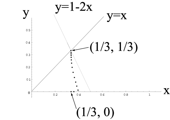
Figure 1: The location of the vacuum configuration with respect to the change of $z_{adj}$ for the parameter set (11). Both axises are normalized as $x=\theta_{1}/2\pi,y=\theta_{2}/2\pi$.

2.1.2 Example II

We have seen that the vacuum configuration is affected by the bare mass and depending on the values of $z_{adj}$, the residual gauge symmetry is different. In our previous example, it is given by either $SU(3)$ or $U(1)\times U(1)$, and we do not have the partial gauge symmetry breaking. Here we will show that such the partial gauge symmetry breaking, which is important in connection with GUT, is possible for an appropriate choice of the parameter.

Let us choose the parameter as

$$(N_{adj},~{}~{}N_{fd},~{}~{}z_{g},~{}~{}z_{fd})=(2,~{}~{}1,~{}~{}1.0,~{}~{}10.0).$$ (13)

We note that the number of flavors is the same as before, but the magnitude of the bare mass, namely, $z_{fd}$ is changed. We study the vacuum structure of the model according to the change of the values of $z_{adj}$. Again the vacuum configuration is obtained by minimizing the effective potential numerically. In Fig.$2$, we depict the location of the vacuum configuration with respect to $z_{adj}$ on the $x$ - $y$ plane.

We observe that

(i) for $0\leq z_{adj}\leq 0.501577$, the vacuum configuration is given by $(x,y)=(1/3,1/3)$, for which the residual gauge symmetry is $SU(3)$,
(ii) if $z_{adj}$ becomes larger than $0.501577$, the configuration starts to move on the line $y=1-2x$ toward $(x,y)=(1/2,0)$. The residual gauge symmetry for the configurations on the line is $SU(2)\times U(1)$. At $z_{adj}\simeq 0.881952$, the vacuum configuration is located at $(x,y)=(1/2,0)$ and stays there for $0.881952\leq z_{fd}\leq 1.11002$,
(iii) for larger values of $z_{adj}\simeq 1.11002$, the configuration $(1/2,0)$ moves on the $x$-axis and finally arrives at $(1/3,0)$ for $z_{adj}\rightarrow\infty$. The residual gauge symmetry for $z_{adj}>1.11002$ is $U(1)\times U(1)$.

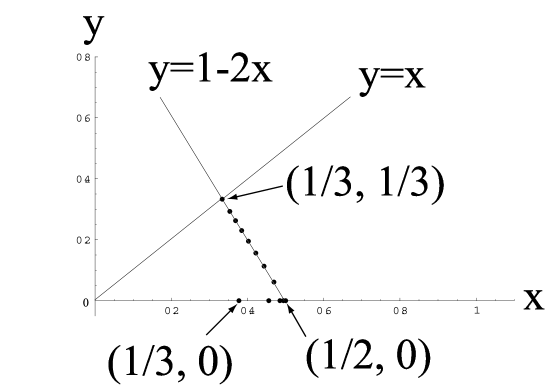
Figure 2: The location of the vacuum configuration with respect to the change of $z_{adj}$ for the parameter set (13). Both axises are normalized as $x=\theta_{1}/2\pi,y=\theta_{2}/2\pi$.

We summarize that

$$\mbox{gauge symmetry breaking patterns}=\left\{\begin{array}[]{ll}0<z_{adj}\leq z_{*1}&\cdots SU(3)\rightarrow SU(3),\\ z_{*1}<z_{adj}\leq z_{*2}&\cdots SU(3)\rightarrow SU(2)\times U(1),\\ z_{adj}>z_{*2}&\cdots SU(3)\rightarrow U(1)\times U(1),\end{array}\right.$$ (14)

where $z_{*1(2)}=0.501577,1.11002$. We also note that the change of the vacuum configuration is continuous and smooth, so that the order of the phase transition is the second order.

The vacuum configuration on the line $\theta_{2}=2\pi-2\theta_{1}$ respects the $SU(2)\times U(1)$ gauge symmetry. This is because for $\theta_{2}=2\pi-2\theta_{1}$

$$W = \mbox{diag}({\rm e}^{i\theta_{1}},{\rm e}^{i\theta_{2}},{\rm e}^{-i(\theta_{1}+\theta_{2})})=\mbox{diag}({\rm e}^{i\theta_{1}},{\rm e}^{2i\pi-2i\theta_{1}},{\rm e}^{i\theta_{1}-2i\pi})$$ (15)

$$= \mbox{diag}({\rm e}^{i\theta_{1}},{\rm e}^{-2i\theta_{1}},{\rm e}^{i\theta_{1}})=\mbox{diag}({\rm e}^{i\theta_{1}},{\rm e}^{i\theta_{1}},{\rm e}^{-2i\theta_{1}}).$$

In the last equality we have made the permutation of the second and third diagonal element. The generators of $SU(3)$ commuting with the above $W$ forms the $SU(2)\times U(1)$. We also observe the configuration on the line $\theta_{2}=\theta_{1}$ is equivalent to the one on the line $\theta_{2}=2\pi-2\theta_{1}$.

Let us comment on the scale of the mass term for $A_{y}$. The zero mode of $A_{y}$ acquires the mass term, which is evaluated from the second derivative of the effective potential at the vacuum configuration. We obtain the effective potential (5) thanks to the supersymmetry breaking due to the bare mass term. We notice that the five-dimensional gauge invariance and supersymmetry forbid the mass term for $A_{y}$. This means that the mass scale for $A_{y}$ must be the one, at which supersymmetry is broken and there is no local gauge invariance in five dimensions. In fact the mass term for $A_{y}$ is estimated, aside from numerical constants, as

$$m_{A_{y}}^{2}\sim N_{deg}N_{f}\times{\bar{g}}^{2}\times\left\{\begin{array}[]{ll}L^{-2}&\mbox{for}\quad ML>1,\\ L^{-2}&\mbox{for}\quad ML\sim 1,\\ M^{2}&\mbox{for}\quad ML\ll 1,\end{array}\right.$$ (16)

where ${\bar{g}}\equiv g/\sqrt{L}$ is the gauge coupling in four dimensions and $N_{deg},N_{f}$ are the on-shell degrees of freedom, the number of flavors, respectively. $M$ stands for the bare mass $M\equiv m_{g,adj,fd}$. We also observe that, as expected, the original supersymmetry protects the mass term for $A_{y}$ against the large quantum correction of $O(L^{-1})$ for the case of $M\ll L^{-1}$. Let us note that the mass is generated through the quantum correction at one-loop level.

3 Conclusions and Discussions

We have studied the gauge symmetry breaking patterns through the Hosotani mechanism in the supersymmetric gauge models in five dimensions. We have introduced the bare mass term for the matter field to break supersymmetry instead of the Scherk-Schwarz mechanism of supersymmetry breaking. And we have studied the effect of the bare mass on the gauge symmetry breaking patterns.

In order to study the vacuum structure of the model, we have fixed some of the parameters because the model contains many parameters. In the paper, we have studied the vacuum structure by changing the values of $z_{adj}$ for the fixed parameter sets given by (11) and (13). As demonstrated in the text, the magnitude of the bare mass actually affects the vacuum structure of the model and changes the gauge symmetry breaking patterns.

We have given two examples, in which the residual gauge symmetry is different. For a parameter set given by (11), the gauge symmetry breaking patterns is (12). On the other hand, for the parameter set (13), it is given by (14) and we have the partial gauge symmetry breaking $SU(3)\rightarrow SU(2)\times U(1)$. The partial gauge symmetry breaking has been found in the models with only massless particles [17]. It should be noted that the partial gauge symmetry breaking is also realized by the appropriate choice of the magnitude of the bare mass. It is interesting to investigate the partial gauge symmetry breaking $SU(5)\rightarrow SU(3)\times SU(2)\times U(1)$, which is important in connection with GUT. We also mention that the order parameter changes smoothly according to the change of $z_{adj}$ in our example, so that the phase transition is the second order.

As far as our numerical analyses are concerned, it seems that the hierarchical structure of the bare mass $z_{g}<z_{fd}$ may be essential for the partial gauge symmetry breaking for the present number of flavors. Needless to say, one needs much more study in order to confirm the statement.

Let us note that there is another way to realize the partial gauge symmetry breaking. In this paper we have considered only the field satisfying the periodic boundary condition. One can introduce the field that satisfy the antiperiodic boundary condition, keeping the singlevaluedness of the Lagrangian density. The mass spectrum is, then, modified as

$${{2\pi}\over L}(n+{\theta_{i}\over{2\pi}})\rightarrow{{2\pi}\over L}(n+{{\theta_{i}-\pi}\over{2\pi}}),$$ (17)

so that, the contribution from the field to the effective potential is given by

$$\bar{V}_{eff}^{anti}=4N_{fd}^{anti}\sum_{n=1}^{\infty}{1\over n^{5}}[2-2D(z_{fd}^{anti},n)]\sum_{i=1}^{N}\cos[n(\theta_{i}-\pi)].$$ (18)

If we take account of the field satisfying the antiperiodic boundary condition and choose the parameters as

$$(N_{adj},~{}~{}N_{fd},~{}~{}N^{anti}_{fd}~{}~{}z_{g},~{}~{}z_{fd},~{}~{}z_{fd}^{anti})=(0,~{}~{}1,~{}~{}1~{}~{},0.0,~{}~{}0.5,~{}~{}0.5)$$ (19)

for example, we can see $(\theta_{1},\theta_{2})=(\pi/3,\pi/3)$ is a vacuum configuration . This shows that in addition to the magnitude of the bare mass, the periodicity of the matter field also changes the gauge symmetry breaking patterns. This is an interesting problem to study further.

It is also important to study the effect of the bare mass on the gauge symmetry breaking patterns in case of orbifold, for instance, $S^{1}/Z_{2}$. In particular, it is interesting to study how the bare mass affects the mass of the Higgs scalar embedded in $A_{y}$ as studied in [12] [22].

Acknowledgements

N.H is supported in part by the Grant-in-Aid for Science Research, Ministry of Education, Science and Culture, Japan, No. 16540258, 16028214, 14740164. K.T would thank the colleagues in Osaka University and the professor Y. Hosotani for valuable discussions. K.T is supported by the $21$st Century COE Program at Osaka University. T.Y thanks the Japan Society for the Promotion of Science for financial support.

References

- [1] Y. Hosotani, Phys. Lett. 126B (1983) 309, Ann. Phys. (N.Y.) 190, 233 (1989).
- [2] N. S. Manton, Nucl. Phys. B158 141 (1979), D. B. Fairlie, Phys. Lett. 82B (1979) 97.
- [3] N. V. Krasinikov, Phys. Lett. 273B (1991) 731, H. Hatanaka, T. Inami and C.S. Lim, Mod. Phys. Lett. A13 (1998) 2601, G. R. Dvali, S. Randjbar-Daemi and R. Tabbash, Phys. Rev. D65 (2002) 064021, N. Arkani-Hamed, A. G. Cohen and H. Georgi, Phys. Lett. 513B (2001) 232, I. Antiniadis, K. Benakli and M. Quiros, New J. Phys. 3, (2001),20.
- [4] M. Kubo, C. S. Lim and H. Yamashita, Mod. Phys. Lett. A17 (2002) 2249.
- [5] L. J. Hall, Y. Nomura and D. R. Smith, Nucl. Phys. B639 (2002) 307.
- [6] G. Burdman and Y. Nomura, Nucl. Phys. B656 (2002) 3.
- [7] N. Haba and Y. Shimizu, Phys. Rev. D67 (2003) 095001.
- [8] C. A. Scucca, M. Serone and L. Silvestrini, Nucl. Phys. B669 (2003) 128.
- [9] I. Gogoladze, Y. Mimura, S. Nandi and K. Tobe, Phys. Lett. 575B (2003) 66.
- [10] C. Csaki, C. Grojean, H. Murayama, L. Pilo and J. Terning, Phys. Rev. D69 (2004) 055006.
- [11] K. Choi, N. Haba, K. S. Jeong, K. Okumura, Y. Shimizu and M. Yamaguchi, J. High Energy Phys.0402, 037 (2004).
- [12] N. Haba, Y. Hosotani, Y. Kawamura and T. Yamashita, J. High Energy Phys.04, 016 (2004).
- [13] N. Haba and T. Yamashita, J. High Energy Phys.0404, 016 (2004).
- [14] Y. Hosotani, S. Noda and K. Takenaga, Phys. Rev. D69 (2004) 125014, hep-ph/0410193.
- [15] A. T. Davies and A. McLachlan, Phys. Lett. 200B (1988) 305, Nucl. Phys. B317 237 (1989), J. E. Hetrick and C. L. Ho, Phys. Rev. D40 (1989) 4085, A. Higuchi and L. Parker, Phys. Rev. D37 (1988) 2853, C. L. Ho and Y. Hosotani, Nucl. Phys. B345 445 (1990), A. McLachlan, Nucl. Phys. B338 188 (1990), K. Takenaga, Phys. Rev. D64 (2001) 066001.
- [16] K. Takenaga, Phys. Lett. 570B (2003) 244.
- [17] H. Hatanaka, Prog. Theor. Phys. 102 (1999) 407, K. Takenaga, Phys. Rev. D66 (2002) 085009.
- [18] J. Scherk and J.H. Schwarz, Phys. Lett. 82B (1979) 60, P. Fayet, Phys. Lett. 159B (1985) 121, Nucl. Phys. B263 87 (1986).
- [19] K. Takenaga, Phys. Lett. 425B (1998) 114, Phys. Rev. D58 (1998) 026004, D61 (2000), 129902(E).
- [20] A. Delgado, A. Pomarol and M. Quiros, Phys. Rev. D60 (1999) 095008.
- [21] N. Haba, K. Takenaga and T. Yamashita, in preparation.
- [22] N. Haba and T. Yamashita, J. High Energy Phys.02, 059 (2004).