Excited states nonlinear integral equations for an integrable anisotropic spin 1 chain

Abstract

We propose a set of nonlinear integral equations to describe on the excited states of an integrable the spin 1 chain with anisotropy. The scaling dimensions, evaluated numerically in previous studies, are recovered analytically by using the equations. This result may be relevant to the study on the supersymmetric sine-Gordon model.

1 Introduction

The 1D spin systems have been providing problems of both physical and mathematical interests. See e.g., [1, 2]. Among them, there exists a family of solvable models of the Heisenberg’s type with spin-$S$ [3, 4]. In this report, we are interested in the excited states of a member in the family, the spin 1 chain with anisotropic interaction.

The recent progress in the study of the integrable system brings forth a powerful machinery, the method of the nonlinear integral equations (NLIE, for short) [5, 6]. The NLIE method has been successfully applied to the study of the XXZ model ($S=\frac{1}{2}$). It clarifies the finite size property of the ground state as well as the scaling behavior of excited states (of corresponding six vertex model [7]). The application is not restricted to the lattice models: it also provides the detailed descriptions of the excited states in the field theoretical models such as the sine-Gordon model[8, 9, 10, 11, 12] and perturbed conformal field theories[13, 14].

The study on the higher spin cases has, however, encountered technical difficulties. This has been resolved in [15] at least for the ground state. There the NLIE, which is relevant to the evaluation of the free energy for arbitrary $S$, is derived for the isotropic case . See also [16] for an interesting application of the result to the $0(4)$ nonlinear sigma model in the limit $S\rightarrow\infty$ .

In this report, we extend the study to excited states of the anisotropic $S=1$ chain . Simple assumptions, suggested by numerical investigations, lead to a set of NLIE which enables the evaluation of energies for arbitrary system size. The proposed NLIE has a structure which seems to be a natural extension of the excited NLIE for the spin $\frac{1}{2}$ case. We will analytically verify the previous observations on some low lying excitations by numerical methods [17, 18].

The result obtained here may be not only relevant in the spin chain problem. Recently the study on the excited states in supersymmetric sine-Gordon model attracts much attentions[19, 20]. It is expected that the proper discretization of the model is given by the inhomogeneous anisotropic spin 1 chain. We thus hope that the current study will shed some light on the analysis of the supersymmetric sine-Gordon model.

2 The model and the assumptions

We are interested in the spin 1 chain with anisotropic interactions. The hamiltonian contains several two-body interactions,

$${\cal H}\negthickspace=\negthickspace\sum_{i=1}^{N}\Bigl{(}\sigma_{i}^{\perp}-(\sigma_{i}^{\perp})^{2}+\cos 2\gamma(\sigma_{i}^{z}-(\sigma_{i}^{z})^{2})-(2\cos\gamma-1)\bigl{(}\sigma_{i}^{\perp}\sigma_{i}^{z}+\sigma_{i}^{z}\sigma_{i}^{\perp}\bigr{)}-4\sin^{2}\gamma(S_{i}^{z})^{2}\Bigr{)}$$ (1)

where a short-hand notation

$$\sigma_{i}=S_{i}\cdot S_{i+1}=\sigma_{i}^{\perp}+\sigma_{i}^{z}$$

is employed. For simplicity, we impose the periodic boundary condition, $S_{N+1}^{a}=S_{1}^{a},a=x,y,z$. The parameter $\gamma$ specifies the anisotropy. Throughout this report, we only consider the range $\gamma<\frac{\pi}{3}$ and exclude $\gamma$ of the form $\gamma=\frac{n\pi}{m}$ with $(m,n)$ co-prime.

We follow the strategy in [15] and start from a integrable 19 vertex model [21, 22]. The 19 vertex model is obtained from the 6 vertex model by the fusion procedure[22, 23]. The latter one is associated to the spin $\frac{1}{2}$ XXZ model while the former corresponds to the spin 1 chain. The strategy is to treat the spin 1 model and the spin $\frac{1}{2}$ model simultaneously. To be more precise, we introduce commuting transfer matrices $T_{1}(x)$ and $T_{2}(x)$ acting on spin 1 quantum space consisting of $N$ sites. The auxiliary space for the former one is given by the spin $\frac{1}{2}$ space while it is spin 1 for the latter.

Their explicit eigenvalues read,

$$T_{1}(z) = \phi(z-i\gamma)\frac{Q(z+i\gamma)}{Q(z)}+\phi(z+i\gamma)\frac{Q(z-i\gamma)}{Q(z)}$$

$$T_{2}(z) = \phi(z-i\frac{\gamma}{2})\phi(z-i\frac{3\gamma}{2})\frac{Q(z+i\frac{3\gamma}{2})}{Q(z-i\frac{\gamma}{2})}+\phi(z-i\frac{\gamma}{2})\phi(z+i\frac{\gamma}{2})\frac{Q(z+i\frac{3\gamma}{2})Q(z-i\frac{3\gamma}{2})}{Q(z+i\frac{\gamma}{2})Q(z-i\frac{\gamma}{2})}$$ (2)

$$+\phi(z+i\frac{\gamma}{2})\phi(z+i\frac{3\gamma}{2})\frac{Q(z-i\frac{3\gamma}{2})}{Q(z+i\frac{\gamma}{2})}$$

$$\phi(z) = \sinh^{N}z$$

Note that in place of standard spectral parameter $u$ , we choose $u=ix$ . The important function $Q$ is given by the Bethe ansatz roots $z_{j},(j=1,\cdots,M)$; $Q(z)=\prod_{j=1}^{M}\sinh(z-z_{j})$. We will denote three terms of $T_{2}(z)$ in (2) by $\lambda_{i}(x),i=1,2,3$.

The eigenvalue $E$ of the Hamiltonian is evaluated though

$$E=\frac{1}{i}\frac{d}{dx}\log T_{2}(x)|_{x\rightarrow-i\gamma/2}.$$ (3)

Thus once if $Q$ is obtained, the evaluation of $E$ is straightforward. This is equivalent to say that, if all locations of the Bethe ansatz roots are known for excited states, then the energy is evaluated. This is, however, a formidable task for large systems. Apart from few lower excitations, it is extremely difficult to find all locations of Bethe ansatz roots.

The most crucial observation in the NLIE formulation is that this task is avoidable. With proper choice of auxiliary functions, one can bypass dealing with a complete set of Bethe ansatz roots; one only has to deal with finite number of complex roots characterizing the excitation[24, 7, 10, 13, 14]. This may break down if very high excitations are of our interest. We nevertheless believe that this method will be efficient for the treatment on excited states which are physically important in the thermodynamic limit.

Let us be more accurate. In the ground state, the Bethe ansatz roots are given by the sea of 2 strings. By a 2 string we mean a pair of Bethe ansatz roots $x_{i}\pm iy_{j}$ with $|y_{j}-\frac{\gamma}{2}|\ll 1$.

We consider excitations for which only a finite number of roots deviate from the sea of 2 strings.

In addition, we will make the following three assumptions.

Assumption 1
There should not be a pair of complex roots $z_{1},z_{2}$ such that $z_{1}-z_{2}$ is a multiple of $\gamma$.

For the string type solutions, it is known that the separation of neighboring roots in a string deviates slightly from $\gamma$ for finite system sizes [25]. Our assumption thus does not contradict with this pattern. It, however, excludes the complete strings[26, 27]. Therefore we should devise another route to deal with the case when $q(={\rm e}^{i\gamma})$ is at roots of unity, which is beyond the present scope.

Assumption 2
The following classification of complex roots , other than 2 strings, are possible.

1. inner roots : $|\Im z_{j}|<\frac{\gamma}{2},j=1,\cdots,M_{I}$

2. close roots: $\frac{\gamma}{2}<|\Im z_{j}|<\frac{3\gamma}{2},j=1,\cdots,M_{C}$

3. wide roots: $\frac{3\gamma}{2}<|\Im z_{j}|<\frac{\pi}{2},j=1,\cdots,M_{W}$

4. self conjugate roots : $|\Im z_{j}|=\frac{\pi}{2},\,j=1,\cdots,M_{p}$.

The above classification has already been proposed in [28] which discusses the excitations in the limit $N\rightarrow\infty$. There a complex conjugate pair of inner roots is referred to as a narrow pair while a pair of close roots is to a intermediate. We adopt a different notation for similar roles played by them in comparison with the spin $\frac{1}{2}$ case. We will sometime denote the locations of inner roots by $s^{\pm}_{j}$, close roots by $c^{\pm}_{j}$, wide pairs by$w^{\pm}_{j}$ and self-conjugate roots by $p_{j}+\frac{\pi}{2}i$. Here the upper index $+(-)$ means its imaginary part being positive (negative).

The zeros of $T_{1}(x)$ and $T_{2}(x)$ play also important parts. The numerical investigation for $N$ up to 8 leads to the remarkable feature.

Assumption 3
The zeros of $T_{1}(x)$ and $T_{2}(x)$ in the strip $\Im x\in[-\gamma/2,\gamma/2]$ distribute exactly on the real axis. We denote their locations by $\theta^{(1)}_{j},(j=1,\cdots,N_{1})$ and by $\theta^{(2)}_{\alpha},(\alpha=1,\cdots,N_{2})$ , respectively.

For example, we plot the zeros of $T_{1}(x)$ and $T_{2}(x)$ for two cases in fig. 1. The state in the left figure in 1 corresponds to an excited state in the singlet sector($M=6$), system size is l $N=6$ chain and with the coupling constant $\gamma=\frac{\pi}{7.5}$. For the state in the right figure in 1, parameters are chosen $M=7,N=8$ and $\gamma=\frac{\pi}{9.5}$. The unit of tics in imaginary direction is normalized to $\frac{\gamma}{2}$. These figures thus clearly support the assumption3, which simplifies the derivation of the nonlinear integral equations drastically.

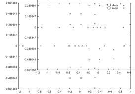
Figure 1: Zeros of $T_{1}(x)$ and $T_{2}(x)$, Left: an excited state in $N=6$ chain $M=6,\gamma=\frac{\pi}{7.5}$ Right: $N=8$ chain $M=7(S_{z}=1),\gamma=\frac{\pi}{9.5}$.

We supplement the explicit locations of corresponding BAE roots.

BAE roots for $N=6$, $M=6$, $\gamma=\frac{\pi}{7.5}$
0.65640208387 $+$1.5707963268 i	-0.53549516834 $+$1.5707963268i
-0.11533405190$+$0.20504539087 i	-0.11533405190$-$0.20504539087i
-0.24721889635	0.35698008462

BAE roots for $N=8$, $M=7$, $\gamma=\frac{\pi}{9.5}$
0.61918637956$+$ 1.5707963268i	-0.10487718381$+$ 1.5707963268i
-0.83691028264$+$ 1.5707963268i	0.29966102387 $-$0.152149003388i
-0.18745636322	0.024363369664
0.29966102387$+$ 0.15214900339 i

3 Auxiliary functions and Sum rules

In this section, we introduce several auxiliary functions which are crucial for our purpose.

Firstly we define the most natural auxiliary function ${\mathfrak{a}}(z)$, defined by

$${\mathfrak{a}}(z)=\frac{\lambda_{2}(z+i\frac{\gamma}{2})}{\lambda_{1}(z+i\frac{\gamma}{2})}=\frac{\lambda_{3}(z-i\frac{\gamma}{2})}{\lambda_{2}(z-i\frac{\gamma}{2})}$$

In view of ${\mathfrak{a}}(z)$, the Bethe ansatz equation can be cast into the form ${\mathfrak{a}}(z_{j})=-1,\qquad(j=1,\cdots,M).$ One also uses its logarithmic form, $Z^{(1)}_{N}(z_{j})=2\pi I_{j}$ , where ${\mathfrak{a}}(z)=\exp(iZ^{(1)}_{N}(z))$, which leads to the root density function formulation in the thermodynamic limit. The first auxiliary function, ${\mathfrak{a}}(z)$, thus has the deep connection to the Bethe ansatz equation and plays the fundamental role in the study of the spin $\frac{1}{2}$ chain. The previous study [15] shows that, unexpectedly, this is not the case for general values of $S$ at their ground states. Instead, the most crucial functions for the ground state for $S=1$ are given by

$$\mathfrak{b}_{1}(x):=\frac{\lambda_{1}(x)+\lambda_{2}(x)}{\lambda_{3}(x)}\qquad\bar{\mathfrak{b}}_{1}(x):=\frac{\lambda_{2}(x)+\lambda_{3}(x)}{\lambda_{1}(x)}$$ (4)

Physically, $\mathfrak{b}_{1}(x)$ is related to the density function associated to the centers of 2-strings.

For a technical reason, we introduce the shifted functions,

$\mathfrak{b}(x)=\mathfrak{b}_{1}(x+i\epsilon)$ $\bar{\mathfrak{b}}(x)=\bar{\mathfrak{b}}_{1}(x-i\epsilon)$ and capital ones $\mathfrak{B}(x)=1+\mathfrak{b}(x)$, $\bar{\mathfrak{B}}(x)=1+\bar{\mathfrak{b}}(x)$. The definition obviously concludes,

$$T_{2}(x) =\phi(x+i\frac{\gamma}{2})\phi(x+i\frac{3\gamma}{2})\frac{Q(x-\frac{3i\gamma}{2})}{Q(x+\frac{i\gamma}{2})}\mathfrak{B}(x-i\epsilon)$$ (5)

$$=\phi(x-i\frac{\gamma}{2})\phi(x-i\frac{3\gamma}{2})\frac{Q(x+\frac{3i\gamma}{2})}{Q(x-\frac{i\gamma}{2})}\bar{\mathfrak{B}}(x+i\epsilon)$$ (6)

and $\mathfrak{B}(x)=0$ when $x=\theta^{(2)}_{j}-i\epsilon$.

In analogy to ${\mathfrak{a}}(z)$ and $Z^{(1)}_{N}(x)$ we introduce $Z^{(2)}_{N}(x):=\frac{1}{i}\log\mathfrak{b}(x)$. In contrast with $Z^{(1)}_{N}(x),$$Z^{(2)}_{N}(x)$ is in general a complex-valued function. We assume that its real part is an almost monotonic increasing function of $x$ and that the imaginary part vanishes when the real part takes integers (half-integers). One then applies the similar argument for the spin $\frac{1}{2}$ [10] to derive the following sum rule,

$$N_{2}=2(S+M_{p})-\frac{2}{\pi}\theta(3\gamma S+\theta(2\gamma S))+2M_{W}+M_{c}$$ (7)

where $\theta(x):=\pi\lfloor\frac{1}{2}+\frac{x}{2\pi}\rfloor$ and $\lfloor x\rfloor$ specifies the integer part of $x$.

The validity of this rule is checked against many examples. The rule is crucial in the determination of the constant term in the NLIE.

We have a remark. The repeated integers are observed for $Z^{(1)}_{N}(x)$, which are attributed to the existence of special holes/roots[10, 11]. Our case studies indicate no symptom of ”special holes/roots” for $Z^{(2)}_{N}(x)$. We therefore dismiss the possibility in this report. Even if they exist, only a small modification will be needed in the following argument.

We need to introduce another pair of auxiliary functions, one of which coincides with $T_{2}$ , apart from the normalization.

$$y_{1}(x):=\frac{T_{2}(x)}{\phi(x-i\frac{3\gamma}{2})\phi(x+i\frac{3\gamma}{2})}\qquad Y_{1}(x):=1+y_{1}(x)$$ (8)

The essential observation to derive the NLIE for $\ln\mathfrak{b}$ remains almost same as the one made in the case of the largest eigenvalue sector of the quantum transfer matrix[15].

We introduce renormalized functions,

$$T^{\vee}_{2}(x)=\frac{T_{2}(x)}{r_{2}(x)}\qquad r_{2}(x):=\prod_{\alpha=1}^{N_{2}}\tanh\frac{\pi}{2\gamma}(x-\theta^{(2)}_{\alpha})$$ (9)

and consider the integral,

$$\int_{\cal C}\frac{d^{2}}{dz^{2}}\log T^{\vee}_{2}(z)e^{-ikz}dz,$$

where ${\cal C}$ encircles the strip of width $\gamma$ (Fig 2) in the counterclockwise manner .

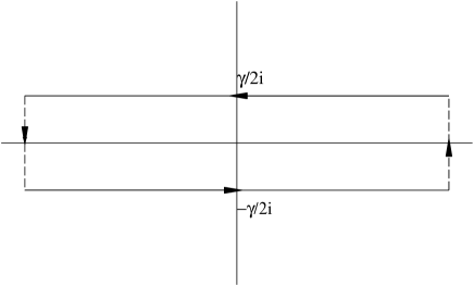
Figure 2: The integration contour ${\cal C}$. The straight line in the lower half plane is termed as ${\cal C}_{\ell}$ while the one in the upper plane is referred to as ${\cal C}_{u}$ after reversing the direction.

Thanks to the renormalization factor, $T^{\vee}_{2}(x)$ contains no zeros or poles inside ${\cal C}$. The Cauchy’s theorem thus concludes

$$0=\int_{C_{\ell}}\frac{d^{2}}{dz^{2}}\log T^{\vee}_{2}(z)e^{-ikz}dx-\int_{C_{u}}\frac{d^{2}}{dz^{2}}\log T^{\vee}_{2}(z)e^{-ikz}dx.$$ (10)

where $C_{\ell},C_{u}$ means the lower and the upper part of the contour, respectively.

One then substitutes $T^{\vee}_{2}$ in terms of $\mathfrak{B}$ for $C_{u}$ and $T^{\vee}_{2}$ in terms of $\bar{\mathfrak{B}}$ for $C_{\ell}$ by utilizing (5 ) and (6 ). This provides the various relations among auxiliary functions in the Fourier space. After straightforward manipulations we find the desired NLIE

$$\ln\mathfrak{b}(x) = C_{b}+iD_{b}(x+i\epsilon)$$ (11)

$$+\int_{-\infty}^{\infty}G_{s}(x-x^{\prime})\ln\mathfrak{B}(x^{\prime})dx^{\prime}-\int_{-\infty}^{\infty}G_{s}(x-x^{\prime}+2i\epsilon)\ln\bar{\mathfrak{B}}(x^{\prime})dx^{\prime}$$

$$+\int_{-\infty}^{\infty}K(x-x^{\prime}-\frac{\gamma}{2}i+i\epsilon)\ln Y_{1}(x^{\prime})dx^{\prime}$$

$$\ln y_{1}(x) = D_{y}(x)+\int_{-\infty}^{\infty}\bigl{(}K(x-x^{\prime}+\frac{\gamma}{2}i-i\epsilon)\ln\mathfrak{B}(x^{\prime})+K(x-x^{\prime}-\frac{\gamma}{2}i+i\epsilon)\ln\bar{\mathfrak{B}}(x^{\prime})\bigr{)}dx^{\prime}$$

where kernel functions read

$$G_{s}(x) = \frac{1}{2\pi}\int_{-\infty}^{\infty}\frac{\sinh(\frac{\pi}{2}-\frac{3\gamma}{2})k}{2\cosh(\frac{\gamma}{2}k)\sinh(\frac{\pi}{2}-\gamma)k}{\rm e}^{ikx}dk$$

$$K(x) = \frac{1}{2\pi}\int_{-\infty}^{\infty}\frac{1}{2\cosh(\frac{\gamma}{2}k)}{\rm e}^{ikx}dk.$$

It is worth mentioning that $G_{s}(x)$ is related to the logarithmic derivative of the soliton-soliton scattering matrix of the sine-Gordan model, and $K(x)$ is a standard kernel function in the thermodynamic Bethe ansatz equation for the RSOS model [29].

The constant $C_{b}$ is found by matching both sides of NLIE at $x\rightarrow-\infty$ and it reads,

$$C_{b}=\pi iS-i\theta(\gamma S).$$ (13)

We remark that, depending on choice of branches, this value is determined only modulo $2\pi i$. This ambiguity can be absorbed into the definitions of branch cut integers.

The driving term in (11) consists of three parts: $D_{b}(x)=D^{(b)}_{\rm bulk}(x)+D^{(b)}_{\rm hole}(x)+D^{(b)}_{\rm roots}(x).$ The first term is identical to the one for the ground state, thus we refer it to as the bulk contribution,

$$D^{(b)}_{\rm bulk}(x)=N\chi_{K}(x)$$

where $\chi^{\prime}_{K}(x)=2\pi K(x)$ and $\chi_{K}(-\infty)=0$. The second consists of two pieces, the contributions of holes of $T_{1}$ and $T_{2}$.

$$D^{(b)}_{\rm hole}(x)=\sum_{j}\chi_{K}(x-\theta^{(1)}_{j})+\sum_{\alpha}\chi(x-\theta^{(2)}_{\alpha})$$

where $\chi(x)$ is an odd primitive of $2\pi G_{s}(x)$ and $\chi(0)=0$. The third term represents the contributions from complex zeros other than 2 strings,

$$D^{(b)}_{\rm roots}(x) = -\sum_{\sigma=\pm,j}\chi(x-(c_{j}^{\sigma}-\sigma\frac{\gamma}{2}i))+\sum_{\sigma=\pm,j}\phi_{\delta}(\frac{x-(w^{\sigma}_{j}-\sigma\frac{\pi}{2}i)}{\eta})+\sum_{j}\phi_{\delta}(\frac{x-p_{j}}{\eta})$$

$$\phi_{\delta}(x):=\frac{1}{i}\log-\frac{\sinh(x-i\delta)}{\sinh(x+i\delta)}$$

and parameters are given by $\delta=\frac{\pi(\pi-3\gamma)}{2(\pi-2\gamma)}$ and $\eta=1-\frac{2\gamma}{\pi}$. The last two summations in (LABEL:Droots) can also be written as

$$-\sum_{\sigma=\pm,j}\chi_{II}(x-(w^{\sigma}_{j}-\sigma i\frac{\gamma}{2}))-\sum_{j}\chi_{II}(x-p_{j}-\frac{\pi-\gamma}{2}i)$$

where we adopt a notation; for any function $f(x)$, $f_{II}(x)=f(x)+f(x-i\gamma{\rm sgn}(\Im x))$ [10].

The driving term for $\ln y_{1}$ lacks the bulk contribution and composed of two terms, $D_{y}(x)=D^{(y)}_{\rm hole}+D^{(y)}_{\rm roots}$. Explicitly,

$$D^{(y)}_{\rm hole}(x)\!=\!i\sum_{\alpha}\chi_{K}(x-\theta^{(2)}_{\alpha}+\frac{\gamma}{2}i)\quad D^{(y)}_{\rm roots}(x)\!=\!-i\sum_{\sigma=\pm,j}\sigma\chi_{K}(x-c^{\sigma}_{j}+\sigma\gamma i).$$

For given locations of excited zeros and holes, eqs. (11) and (LABEL:y1NLIE2) fix the values of auxiliary functions (modulo $exp(2\pi i)$). Then the evaluation of energy spectra for any $N$ is immediate by the following expression,

$$E=e_{0}+e_{\rm hole}+e_{\rm roots}+e_{B}.$$ (16)

In the above $e_{0}$ denotes the bulk ground state energy $e_{0}=-N(\cot\gamma+\cot 2\gamma)$. The second term $e_{\rm hole}$ stands for the excitation energy for a hole,

$$e_{\rm hole}=\sum_{j}e(\theta^{(2)}_{j}),\qquad e(x):=\frac{\pi}{\gamma}\frac{1}{\cosh\frac{\pi}{\gamma}x}.$$

Among the contributions from complex excitations, the one from the close roots appears here explicitly,

$$e_{\rm roots}=-\sum_{\sigma=\pm,j}e(c^{\sigma}_{j}-i\sigma\frac{\gamma}{2}).$$

This phenomenon is also observed for the spin $\frac{1}{2}$ case [10] for $\gamma\leq\frac{\pi}{2}$.

The last term contains implicit contributions from all excitations, and it is given by

$$e_{B}=\frac{1}{i}\int K^{\prime}(x-x^{\prime}-i\epsilon+i\frac{\gamma}{2})|_{x\rightarrow-i\gamma/2}\ln\mathfrak{B}(x^{\prime})dx^{\prime}+\frac{1}{i}\int K^{\prime}(x-x^{\prime}+i\epsilon-i\frac{\gamma}{2})|_{x\rightarrow-i\gamma/2}\ln\bar{\mathfrak{B}}(x^{\prime})dx^{\prime}.$$

The locations of complex roots and holes are, however, not given a priori. Therefore an improvement of the set of NLIE is necessary so as to make the evaluation of these locations possible. To resolve this, we need the NLIE for $\ln\mathfrak{a}$ with a general complex argument $z$.

The derivation of the NLIE can be done in two ways. One starts from the derivation for real $z$, then apply the analytic continuation argument in [10] to derive the equation valid for $y$ with larger complex parts. The procedure is straightforward but for a small technical difficultly which does not show up in the spin $\frac{1}{2}$ problem. Alternatively, one can start directly from $y$ with larger complex part, apply carefully the following simple lemma 1 to reach desired NLIE.

Lemma 1

We define, for a smooth function $f(z)$, its ”Fourier transformation” by

$$f_{y}[k]=\frac{1}{2\pi}\int_{-\infty}^{\infty}f(x+iy){\rm e}^{-ikx}dx.$$ (17)

with $z=x+iy$.

Suppose $f(z)$ has a pole at $z=z_{0}$ with the residue $r$ and analytic elsewhere. For $\Im z_{0}>0$ then

$$f_{y}[k]=\begin{cases}f[k]{\rm e}^{-ky}&0\leq y<\Im z_{0}\\ (f[k]-ir{\rm e}^{-ikz_{0}}){\rm e}^{-ky}&y>\Im z_{0}\\ \end{cases}$$

Similarly for $\Im z_{0}<0$

$$f_{y}[k]=\begin{cases}f[k]{\rm e}^{-ky}&\Im z_{0}\leq y<0\\ (f[k]+ir{\rm e}^{-ikz_{0}}){\rm e}^{-ky}&y<\Im z_{0}\\ \end{cases}.$$

We have derived the following equations by these two manners and checked that they lead to identical results.

A moment consideration convinces us that we need to treat the equations, at least by three separate regimes for positive imaginary values of $z$.

For the simplest case, $\Im z\in[0,\frac{\gamma}{2})$ , the NLIE reads

$$\ln\mathfrak{a}(z)=C_{a}+iD_{a}(z)-\int_{-\infty}^{\infty}K(z-x^{\prime}-i\epsilon)\ln\mathfrak{B}dx^{\prime}+\int_{-\infty}^{\infty}K(z-x^{\prime}+i\epsilon)\ln\bar{\mathfrak{B}}dx^{\prime}$$ (18)

where the constant and drive term are given by

$$C_{a} = 2i\theta(2\gamma S)-i\theta(3\gamma S+\theta(2\gamma S))$$

$$D_{a}(z) = \sum_{\sigma=\pm,j}\chi_{K}(z-(c_{j}^{\sigma}-\sigma\frac{\gamma}{2}i))-\sum_{\alpha}\chi_{K}(z-\theta^{(2)}_{\alpha}).$$

The equation ceases to be valid as $\Im z$ crosses $\frac{\gamma}{2}$ due to the singularities existing in the kernel functions of the above equation. Taking account of the modification due to them, we find the equation for $\Im z\in(\frac{\gamma}{2},\frac{3\gamma}{2})$

$$\ln\mathfrak{a}(z)\! - \!\ln(1+\frac{1}{\mathfrak{a}(z-i\gamma)})\!=\!-C_{b}-iD_{b}(z-i\frac{\gamma}{2})$$ (19)

$$- \!\int_{-\infty}^{\infty}G_{s}(z-i\frac{\gamma}{2}-x^{\prime}-i\epsilon)\ln\mathfrak{B}dx^{\prime}+\int_{-\infty}^{\infty}G_{s}(z-i\frac{\gamma}{2}-x^{\prime}+i\epsilon)\ln\bar{\mathfrak{B}}dx^{\prime}$$

$$+ \!\int_{-\infty}^{\infty}K(z-x^{\prime})\ln(1+y_{1}(x^{\prime}))dx^{\prime}$$

The simultaneous evaluation of $\mathfrak{a}(z)$ at different strips is thus necessary within this framework. When $z=i\gamma$, some spurious singularities appear in the rhs, which causes some numerical problems. We hope to report on the remedy in a separate communication.

The last case, $\Im z\in(\frac{3\gamma}{2},\frac{\pi}{2})$, the equation takes again a simpler form,

$$\ln\mathfrak{a}(z)=i\widetilde{D_{a}}(z)-\int_{-\infty}^{\infty}G_{s}^{II}(z-i\frac{\gamma}{2}-x^{\prime}-i\epsilon)\ln\mathfrak{B}dx^{\prime}+\int_{-\infty}^{\infty}G_{s}^{II}(z-i\frac{\gamma}{2}-x^{\prime}+i\epsilon)\ln\bar{\mathfrak{B}}dx^{\prime}$$ (20)

Note that integration constant is null modulo $2\pi i$ and the drive term reads,

$$\widetilde{D_{a}}(z) = \sum_{\alpha}\phi_{\delta}(\frac{z-i\frac{\pi}{2}-\theta^{(2)}_{\alpha}}{\eta})-\sum_{\sigma=\pm,j}\phi_{\delta}(\frac{z-i\frac{\pi}{2}-(c^{\sigma}_{j}-\sigma\frac{\gamma}{2}i)}{\eta})$$

$$-\sum_{\sigma=\pm,j}\phi^{II}_{\delta}(\frac{z-i\frac{\gamma}{2}-(w^{\sigma}_{j}-\sigma\frac{\pi}{2}i)}{\eta})-\sum\phi^{II}_{\delta}(\frac{z-i\frac{\gamma}{2}-p_{j}}{\eta})$$

Although these three NLIE for $\ln{\mathfrak{a}}$ take rather involved forms, their meaning is simple: once $\ln\mathfrak{B},\ln\bar{\mathfrak{B}}$ and $\ln Y$ are known on the real axis, the NLIE yield the evaluation of $\ln{\mathfrak{a}}$ at arbitrary $z$. Again, we have checked the validity of these NLIE at various points in the complex plane.

As noted above, the locations of complex roots and holes are determined by ”quantization” conditions

$$\ln\mathfrak{a}(\theta^{(1)}_{j}) =(2I^{(a)}_{j}+1)\pi i, \ln\mathfrak{b}(\theta^{(2)}_{\alpha}-i\epsilon) =(2I^{(b)}_{\alpha}+1)\pi i$$

$$\ln\mathfrak{a}(c^{\pm}_{j}) =(2I^{(c^{\pm})}_{j}+1)\pi i, \ln\mathfrak{a}(w^{\pm}_{j}) =(2I^{(w^{\pm})}_{j}+1)\pi i,$$

$$\ln\mathfrak{a}(p_{j}+\frac{\pi}{2}i) =(2I^{(p)}_{j}+1)\pi i.$$ (21)

To be precise the NLIE still leaves $2\pi i$ ambiguity as remarked in the above . Thus one has to be careful in the choice of branch cuts. We will present several examples of proper choices in the next section.

The set of properly chosen integers then fixes the locations of complex roots and holes, thereby the energy spectra. In this sense, the NLIE characterizes the finite size spectra completely.

4 Low lying Excitations in the thermodynamic limit

For an illustration, we consider the energy levels of some low lying excitations in the thermodynamic limit. We consider the weak anisotropy $\gamma\rightarrow 0$ case. As shown in [6, 24, 10], the scaling behavior of these levels can be evaluated without solving the NLIE explicitly.

The contribution to the excited spectra mainly comes from the left and right extremes of roots distribution. In the limit, $N\rightarrow\infty$, these two contributions are almost decoupled.

The energy scales as

$$E\sim N\epsilon_{0}+\frac{1}{N}\triangle E$$

where $\epsilon_{0}$ denotes the bulk ground state energy. The scaling energy $\triangle E$ is given by the sum of left and right contributions, $\triangle E=\triangle E_{+}+\triangle E_{-}$. We conveniently introduce scaling functions,

$$a_{\pm}(x) =\mathfrak{a}(\pm\frac{\gamma}{\pi}(x+\ln N)), A_{\pm}(x) =1+a_{\pm}(x)$$

$$b_{\pm}(x) =\mathfrak{b}(\pm\frac{\gamma}{\pi}(x+\ln N)), B_{\pm}(x) =1+b_{\pm}(x)$$

$$y_{\pm}(x) =y_{1}(\pm\frac{\gamma}{\pi}(x+\ln N)), Y_{\pm}(x) =1+y_{\pm}(x)$$

Similarly, to holes near the left (right) extremes, we associate the new locations $\theta^{+}$($\theta^{-}$),

$$\theta^{\pm}_{j}=\pm\frac{\pi}{\gamma}\theta^{(2)}_{j}-\log N$$ (22)

Then the left/right contributions are explicitly written as

$$\triangle E_{\pm}=\frac{2\pi}{\gamma}\sum_{j}{\rm e}^{-\theta^{\pm}_{j}}\pm\frac{1}{i\gamma}\int{\rm e}^{-(x\pm i\epsilon^{\prime})}\log B_{\pm}dx\mp\frac{1}{i\gamma}\int{\rm e}^{-(x\mp i\epsilon^{\prime})}\log{\bar{B}}_{\pm}dx$$ (23)

where $\epsilon^{\prime}=\frac{\pi}{\gamma}\epsilon$. In the following discussion, it is irrelevant thus we set $\epsilon^{\prime}\rightarrow 0$ for notational simplicity.

The NLIE also can be transformed into scaling forms. We prepare associated kernel functions and drive functions,

$$K^{\gamma}(x) =\frac{\gamma}{\pi}K(\frac{\gamma}{\pi}x), G^{\gamma}(x) =\frac{\gamma}{\pi}G_{s}(\frac{\gamma}{\pi}x)$$

$$\chi^{\gamma}(x) :=\chi(\frac{\gamma}{\pi}x), \chi^{\gamma}_{K}(x) :=\chi_{K}(\frac{\gamma}{\pi}x)$$

Then the set of resultant NLIE takes the form,

$$\ln b_{\pm}(x)= \mp 2i{\rm e}^{-x}+C^{\pm}_{b}+iD^{\pm}_{b}(x)+\int G^{\gamma}(x-x^{\prime})\ln B_{\pm}(x^{\prime})dx^{\prime}-\int G^{\gamma}(x-x^{\prime})\ln{\bar{B}}_{\pm}(x^{\prime})dx^{\prime}$$

$$+\int K^{\gamma}(x-x^{\prime}\mp\frac{\pi}{2}i)\ln Y_{\pm}(x^{\prime})dx^{\prime}$$

$$\ln y_{\pm}(x)= C^{\pm}_{y}+D^{\pm}_{y}(x)+\int K^{\gamma}(x-x^{\prime}\pm i\frac{\pi}{2})\ln B_{\pm}(x^{\prime})dx^{\prime}$$

$$+\int K^{\gamma}(x-x^{\prime}\mp i\frac{\pi}{2})\ln{\bar{B}}_{\pm}(x^{\prime})dx^{\prime}.$$

Those scaling NLIE for $\ln a_{\pm}$ have similar but more involved forms. We only write the case $\Im x\in[0,\frac{\gamma}{2})$,

$$\ln a_{\pm}(x)=C_{a}^{\pm}+iD_{a}^{\pm}-\int K^{\gamma}(x-x^{\prime})\log B_{\pm}(x^{\prime})dx^{\prime}+\int K^{\gamma}(x-x^{\prime})\log\bar{B}_{\pm}(x^{\prime})dx^{\prime}$$

The constants and $D$ functions in the above depend on the choice of specific state of interest and choice of branch cut integers. Below we consider simple examples for which the results of numerical studies are available.

Example 1:

We consider the lowest excitation in the sector $S_{z}=1$. It is shown numerically that the $N-2$ zeros of $Q(x)$ form the sea of the two strings and the last zero is located at the origin[17, 18]. In the strip $\Im x\in[-\frac{\gamma}{2},\frac{\gamma}{2}]$, $T_{1}$ possesses no zeros while two zeros of $T_{2}$ are located on the real axis. We denote their scaled locations (22) by $\theta^{\pm}$.

The drive terms in this case are found to be,

$$C^{\pm}_{b} =\mp(\pi-\delta)i, D^{\pm}_{b} =\pm\chi^{\gamma}(x-\theta^{\pm})$$

$$C^{\pm}_{y} =\pm\pi i, D^{\pm}_{y} =\pm i\chi^{\gamma}_{K}(x-\theta^{\pm}\pm\frac{\pi}{2}i).$$

We conveniently choose the quantization conditions, $\log b_{\pm}(\theta^{\pm})=\mp(2I^{\pm}+1)\pi$. The locations of holes then satisfy

$${\rm e}^{-\theta^{\pm}} = \mp\frac{1}{2i}\Bigl{(}-(2\pi I^{\pm}+\delta)i-\int G^{\gamma}(\theta^{\pm}-x)\ln B_{\pm}(x)dx$$ (24)

$$\phantom{aaa}+\int G^{\gamma}(\theta^{\pm}-x)\ln{\bar{B}}_{\pm}(x)dx-\int K^{\gamma}(\theta^{\pm}-x\mp\frac{\pi}{2}i)\ln Y_{\pm}(x)dx\Bigr{)}$$

Our choice of $C^{\pm}_{b}$ and of the branch cut integers leads to $I^{\pm}\geq 0$ in the present case. By substituting (24) into (23), we present $\triangle E_{\pm}$ only in terms of auxiliary functions,

$$\triangle E_{\pm} = \frac{1}{i\gamma}\Bigl{(}\pm\int{\rm e}^{-x}\log B_{\pm}dx\mp\int{\rm e}^{-x}\log{\bar{B}}_{\pm}dx+(2\pi^{2}I^{\pm}+\delta\pi)i$$ (25)

$$\phantom{aaa}\pm\pi\int G^{\gamma}(\theta^{\pm}-x)\ln B_{\pm}(x)dx\mp\pi\int G^{\gamma}(\theta^{\pm}-x)\ln{\bar{B}}_{\pm}(x)dx$$

$$\phantom{aaa}\pm\int K^{\gamma}(\theta^{\pm}-x\mp\frac{\pi}{2}i)\ln Y_{\pm}(x)dx\Bigr{)}$$

The standard dilogarithm trick leads to the explicit values of desired integrals,

$$4i\Bigl{(}\pm\int{\rm e}^{-x}\log B_{\pm}dx\mp\int{\rm e}^{-x}\log{\bar{B}}_{\pm}dx$$

$$\phantom{aa}\pm\pi\int G^{\gamma}(\theta^{\pm}-x)\ln B_{\pm}(x)dx\mp\pi\int G^{\gamma}(\theta^{\pm}-x)\ln{\bar{B}}_{\pm}(x)dx$$

$$\phantom{aa}\pm\pi\int K^{\gamma}(\theta^{\pm}-x\mp\frac{\pi}{2}i)\ln Y_{\pm}(x)dx\Bigr{)}$$

$$\phantom{aa}\pm(\pi-2\delta)i\bigl{(}\log B_{\pm}(\infty)-\log{\bar{B}}_{\pm}(\infty)\bigr{)}\mp i\pi\log Y_{\pm}(\infty)$$

$$=\int(\log b_{\pm})^{\prime}\log B_{\pm}dx-\int\log b_{\pm}(\log B_{\pm})^{\prime}dx+\int(\log{\bar{b}}_{\pm})^{\prime}\log{\bar{B}}_{\pm}dx-\int\log{\bar{b}}_{\pm}(\log{\bar{B}}_{\pm})^{\prime}dx$$

$$\phantom{aa}+\int(\log y_{\pm})^{\prime}\log Y_{\pm}dx-\int(\log y_{\pm}\mp\pi i)(\log{Y}_{\pm})^{\prime}dx$$ (26)

where we have used $\chi^{\gamma}_{K}(\infty)=\pi$ It is worth mentioning the asymptotic values

$$b_{\pm}(-\infty) =0 {\bar{b}}_{\pm}(-\infty) =0$$

$$y_{\pm}(-\infty) =-1$$

$$b_{\pm}(\infty) =\frac{1+{\rm e}^{\mp 2i\gamma}}{{\rm e}^{\pm 2i\gamma}} {\bar{b}}_{\pm}(\infty) =\frac{1+{\rm e}^{\pm 2i\gamma}}{{\rm e}^{\mp 2i\gamma}}$$

$$y_{\pm}(\infty) =1+2\cos 2\gamma.$$

Using these values and by the change of integration variables, we find that the rhs of (26) is given by the dilogarithm functions,

$$2L_{+}(b_{\pm}(\infty))+2L_{+}(b_{\pm}(\infty))+2L_{+}(y_{\pm}(\infty))-2L_{+}(1)+2L(1)+2L_{+}(1)\mp\pi i\log Y_{\pm}(\infty)$$ (27)

Explicit definitions are as follows.

$$L_{+}(x) := \frac{1}{2}\int_{0}^{x}(\frac{\log(1+y)}{y}-\frac{\log y}{1+y})dy,$$

$$L(x) := -\frac{1}{2}\int_{0}^{x}(\frac{\log(1-y)}{y}+\frac{\log y}{1-y})dy$$

The scaling energy $\triangle E$ is divided into two parts $\triangle E=\triangle E_{1}+\triangle E_{2}$. The former brings the central charge $\triangle E_{1}=\frac{\pi v}{6}c$ while the second is related to the scaling dimension, $\triangle E_{2}=2\pi vX$. The sound velocity is readily evaluated $v=\frac{\pi}{\gamma}$.

It is easily shown that the sum of the first four terms in (27) remains constant for small $\gamma$. Thus the dilogarithm formula, utilized in the study of the ground state [15] in the rational case ($\gamma\rightarrow$ 0), is also applicable. We identify these terms as the contribution to $\triangle E_{1}=\frac{\pi v}{6}c$. This lead to the correct central charge $\frac{3}{2}$.

Evaluating the remaining contributions, we find,

$$\triangle E_{2}=\frac{2\pi^{2}}{\gamma}(I_{+}+I_{-}+X_{c}+\frac{1}{8})$$

where $X_{c}=\frac{\pi-2\gamma}{4\pi}$. Therefore, by choosing the minimal value $I_{+}=I_{-}=0$, the above calculation recovers the desired scaling dimension, $X=X_{c}+\frac{1}{8}$ [17, 18].

Example 2:

Let us consider another excitation in the sector $S_{z}=1$. The $N-2$ zeros of Q function again form the sea of the two strings while the last zero is located at $\frac{\pi}{2}i$. In this case, $T_{1}(x)$ possesses 2 zeros on the real axis while $T_{2}(x)$ does 4 zeros. We denote corresponding scaling locations by $\xi^{\pm}$ for zeros of $T_{1}(x)$ and $\theta^{\pm}_{j},(j=1,2)$ for those of $T_{2}(x)$. In this case it is convenient to introduce $\chi^{+}_{K}(x):=\chi^{\gamma}_{K}(x)-\pi$ so that $\chi^{+}_{K}(\infty)=0$.

Then the drive terms are then given by,

$$C^{\pm}_{b} =\mp\pi i D^{\pm}_{b} =\pm\sum_{j}\chi^{\gamma}(x-\theta^{\pm}_{j})\pm\chi^{+}_{K}(x-\xi^{\pm})$$

$$C^{\pm}_{y} =0 D^{\pm}_{y} =\pm i\sum_{j}\chi^{+}_{K}(x-\theta^{\pm}_{j}\pm\frac{\pi}{2}i)$$

$$C^{\pm}_{a} =0 D^{\pm}_{a} =\mp\sum_{j}\chi^{+}_{K}(x-\theta^{\pm}_{j})$$

The quantization conditions read

$$\log b^{\pm}(\theta^{\pm}_{j})=\mp(2I^{\pm}_{j}+1)\pi\qquad\log a^{\pm}(\xi^{\pm})=\pm(2J^{\pm}+1)\pi$$

One easily verifies $I^{\pm}_{j},J^{\pm}\geq 0$.

The quantization condition for $\log b^{\pm}$ leads to an expression analogous to (24). This time, however, the rhs contains $\frac{1}{2}\sum_{j}\chi^{+}_{K}(\theta^{\pm}_{j}-\xi^{\pm})$. The quantization condition for $\log a^{\pm}$ enables us to represent this by integrals,

$$\sum_{j}\chi^{+}_{K}(\theta^{\pm}_{j}-\xi^{\pm})=-\pi\pm\frac{1}{i}\int K^{\gamma}(\xi^{\pm}-x)\log B_{\pm}(x)dx\mp\frac{1}{i}\int K^{\gamma}(\xi^{\pm}-x)\log\bar{B}_{\pm}(x)dx$$ (28)

We used a simple relation $\chi^{+}_{K}(x)+\chi^{+}_{K}(-x)=-\pi$ and put $J^{\pm}=0$.

We then proceed as example 1 and obtain the same $\triangle E_{1}$ and

$$\triangle E_{2}=\frac{2\pi^{2}}{\gamma}\bigl{(}1+\frac{\gamma}{\pi(\pi-2\gamma)}\bigr{)}=\frac{2\pi^{2}}{\gamma}\bigl{(}X_{c}+\frac{1}{16X_{c}}+\frac{1}{2}\bigr{)}$$

where we choose $I^{\pm}_{j}=j-1$. This again coincides with the numerical result [17].

We also analyzed several examples in the different spin sectors, and checked that the results all recovered the desired values. We, however omit further discussions for brevity.

5 Discussion and Summary

In this report, we derive a set of NLIE which characterizes excited state spectra of the spin 1 chain with anisotropic interactions. The equations are tested numerically against exact data. Some desired scaling dimensions are derived analytically for some low excitations.

Finally, we comment on an implication of the result obtained here. Through the light cone approach[30, 31], the inhomogeneous version of the spin 1 chain, or the 19 vertex model will be the proper candidate for the discrete analogue of the supersymmetric sine-Gordon model . The latter’s excited spectra have been attracted attentions recently[20] . A proper deformation of the NLIE obtained in this paper may be useful in such investigations. Assume that the several conjectures on the analytic properties in the spin chain problem are also valid for supersymmetric sine-Gordon model. Then it is readily shown that we reach the almost same nonlinear integral equations. The ”bulk” driving term of $\log{\mathfrak{b}}$ should be then replaced by $mL\sinh\frac{\pi}{\gamma}x$ where $mL$ is related to the inhomogeneity $\Lambda$ by $mL=2N\exp(-\frac{\pi}{\gamma}\Lambda)$. We however avoid drawing a conclusion in haste as it requires careful analytic and numerical checks; the consistency to the $S-$matrix picture in [32], for instance. We hope to report this in a near future, together with complete discussion on the conformal limit.

Acknowledgements

The author would like to thank C. Ahn and F. Ravanini for discussions, C.Dunning for the critical reading of the manuscript, P.E. Dorey and J.M. Martins for their interest. The work of JS has been supported by a Grant-in-Aid for Scientific Research from the Ministry of Education, Culture, Sports and Technology of Japan, no. 14540376.