CU-TP-1122

ITFA-2004-49

De Sitter Holography with a Finite Number of States

Maulik Parikh and Erik Verlinde

¹ Department of Physics, Columbia University, New York, NY 10027

¹ Physics Department, University of Amsterdam, The Netherlands

Abstract

We investigate the possibility that, in a combined theory of quantum mechanics and gravity, de Sitter space is described by finitely many states. The notion of observer complementarity, which states that each observer has complete but complementary information, implies that, for a single observer, the complete Hilbert space describes one side of the horizon. Observer complementarity is implemented by identifying antipodal states with outgoing states. The de Sitter group acts on S-matrix elements. Despite the fact that the de Sitter group has no nontrivial finite-dimensional unitary representations, we show that it is possible to construct an S-matrix that is finite-dimensional, unitary, and de Sitter-invariant. We present a class of examples that realize this idea holographically in terms of spinor fields on the boundary sphere. The finite dimensionality is due to Fermi statistics and an ‘exclusion principle’ that truncates the orthonormal basis in which the spinor fields can be expanded.

1 Introduction

Suppose we had the holographic formulation of quantum gravity or string theory in asymptotic de Sitter space – how would we recognize it as such? Experience with Matrix theory and AdS/CFT suggests that the answer is: through the symmetries of de Sitter space. In all known examples of holography, bulk isometries appear as symmetries of the boundary theory. For example, in AdS/CFT, the presence of five-dimensional anti-de Sitter space can be deduced from the dual theory’s $O(2,4)$ conformal symmetry. This idea has been used to propose that $d$-dimensional de Sitter space is holographically dual to a $d-1$ dimensional boundary theory which has the $O(1,d)$ de Sitter isometry group as a symmetry [1]. But, unlike AdS, de Sitter space has cosmological horizons. These horizons have finite area, and hence lead to a finite de Sitter entropy. There are various interpretations of the finiteness of the de Sitter entropy, but one possibility is that it indicates that the Hilbert space of the holographic dual has only a finite number of states [2, 3]. We will consider this strong version of the holographic principle here.

Now, there is an apparent tension between the de Sitter group and the finiteness of the number of states. This is because the de Sitter group is noncompact, and there is an old theorem that says that only compact groups have nontrivial finite-dimensional representations that are unitary. If the Hilbert space is finite, it cannot furnish a nontrivial unitary representation of the de Sitter group. There have thus been claims that de Sitter space has no holographic dual [4], or that the symmetry group is not the de Sitter group [5].

Nevertheless, in this paper we will try to have our cake and eat it too. Namely, we will consider the possibility that there is a holographic description of de Sitter space that is unitary, respects the symmetries of de Sitter space, and yet has only a finite number of states. Our description is motivated by the principle of observer complementarity [6, 7, 8, 9]. One formulation of this principle asserts that every single observer has complete information; there is no need to consider states or events that live or happen outside the observer horizon. For a given observer the Hilbert space consists only of states that are accessible to him or her; these states are sufficient to describe all events that take place inside the observer horizon. The measurable observables are the S-matrix elements that give the probabilities for these events. For unitarity it is then sufficient that the Hilbert space contains states with positive norm, and that the S-matrix be unitary. The clash between unitarity and the finiteness of the number of states is removed because the Hilbert space associated to one observer does not have to be a representation of the full de Sitter group, but only of the compact subgroup that leaves the horizon invariant.

However, different observers are related by the de Sitter group and, in some sense, should be equivalent. How, then, should we implement de Sitter symmetry? We propose that the de Sitter group, even though it does not act on individual states, transforms the elements of the S-matrix. De Sitter invariance implies that the S-matrix respects the symmetries of de Sitter space, just as the S-matrix in Minkowski space respects Poincaré symmetries. In other words, the tensor product of in and out Hilbert spaces should form a representation of the de Sitter group in such a way that the tensor product state corresponding to the S-matrix is invariant. The in and out Hilbert spaces do not by themselves form representations of the de Sitter group because they only form representations of the group that preserves the horizon. The requirement of de Sitter invariance of the tensor product states relates different S-matrix elements and leads to selection rules that reflect the underlying de Sitter symmetry.

The aim of this paper is to present a concrete realization of these ideas by constructing an infinite class of finite-dimensional Fock spaces based on spinor representations of the de Sitter group. This paper is organized as follows. After a brief review of the de Sitter group in section 2, we present the main idea behind the construction in section 3. The finitely many Fock states corresponding to a static patch of de Sitter space do not form representations of the de Sitter group but only of the (compact) rotation subgroup that preserves the observer’s horizon. Global de Sitter space is described by a tensor product of two copies of the Fock space, one corresponding to each of an antipodal pair of observers. The key point is that there are states in the tensor product space that are de Sitter-invariant. In section 4, we make the abstract discussion concrete by presenting two constructions of a finite-dimensional Fock space. In the first construction, the dual theory is based on Dirac spinors. This is perhaps the simplest toy model of de Sitter space [10]. A more general construction, presented in section 5, elevates the Dirac spinors to a spinor field theory living on a sphere. It is manifestly holographic in that the sphere can be thought of as the boundary of de Sitter space. Moreover, it allows representations that, while finite, can be arbitrarily large. In section 6, we identify the de Sitter-invariant states in the tensor product of the antipodal Fock spaces. These singlet states are the key to implementing the de Sitter symmetry. We argue that, by making an antipodal identification of de Sitter space, the two Fock spaces can be thought of as the space of initial and final states. The invariant states can then be reinterpreted as de Sitter-invariant S-matrix elements. Section 7 is a brief illustration of how observer complementarity works in practice.

We mention here that an alternate approach with the same goal in mind would be to q-deform the de Sitter group [11, 12]. In particular, there exist finite and unitary principal series representations of the cyclically q-deformed de Sitter group.

2 The de Sitter Group and the Little Group

Let us briefly review the symmetries of de Sitter space [13, 14]. De Sitter space can be represented as a timelike hyperboloid embedded in Minkowski space:

$$-{X^{0}}^{2}+{X^{1}}^{2}\dots+{X^{d}}^{2}=+R^{2}\;,$$ (1)

where $X^{I}$ are Cartesian embedding coordinates. In this form, the $O(1,d)$ isometry group of $d$-dimensional de Sitter space is manifest; the $d$-dimensional de Sitter group is therefore the Lorentz group in $d+1$ dimensions. The Lorentz generators are

$$M_{IJ}=-i(X_{I}\partial_{J}-X_{J}\partial_{I})\;.$$ (2)

Now consider a geodesic observer in de Sitter space. Such an observer moves along a worldline which, in the Minkowski embedding space, is traced by a trajectory of constant acceleration. This worldline is generated by boosts. Without loss of generality, let the observer stay at the north pole, which we take to be in the positive $X^{d}$ direction. Then the Hamiltonian is

$$H=i\left(X^{0}{\partial\over\partial{X^{d}}}+X^{d}{\partial\over\partial X^{0}}\right)\;.$$ (3)

The generators that leave the observer’s worldline invariant are the rotations about the axis connecting the poles as well as the time translation operator. Together these form the observer’s little group $O(d-1)\times R$. Note that since the rotation group $O(d-1)$ is compact, it admits finite-dimensional unitary representations.

Indeed, this group appears also for a nongeodesic observer. The past and future horizons of an observer are completely determined by specifying a point on the sphere at $\mathcal{I}^{-}$ and another on the sphere at $\mathcal{I}^{+}$. We can just consider two points on a single sphere. Then the generators that correspond to rotations in Minkowski space move both these points while keeping their angular separation fixed. The boosts also move the points but change their angular separation. By means of de Sitter symmetries we can set the points to be the two poles of the sphere. On the sphere, the de Sitter group acts as the Euclidean conformal group $O(1,d)$. It is clear that the transformations that leave the poles invariant consist of the rotations about the axis formed by the poles, as well as the dilation operation. Hence the group that preserves the horizon is just $O(d-1)\times R$.

As the rotation group $O(d-1)$ will play a key role in what follows, it is convenient to relabel the de Sitter algebra in terms of indices $i,j$ that run from 1 to $d-1$:

$$J_{ij}\equiv M_{ij}\qquad P_{i}\equiv M_{di}\qquad K_{i}\equiv M_{0i}\qquad H\equiv M_{0d}\;.$$ (4)

Here $J_{ij}$ generate the rotation group $SO(d-1)$, $P_{i}$ are momentum operators, $K_{i}$ are the boosts, and $H$ is the generator of time translations. Then, in terms of these generators, the de Sitter algebra consists of the $so(d-1)$ rotation algebra,

$${[J_{ij},J_{km}]}=-i\left(\delta_{jk}J_{im}-\delta_{ik}J_{jm}-\delta_{jm}J_{ik}+\delta_{im}J_{jk}\right)\;,$$ (5)

as well as

$${[J_{ij},P_{k}]}\;\;= -i\delta_{jk}P_{i}+i\delta_{ik}P_{j}\qquad\qquad{[P_{i},P_{j}]} =+iJ_{ij}$$

$${[J_{ij},K_{k}]}\;\;= -i\delta_{jk}K_{i}+i\delta_{ik}K_{j}\qquad\;\;\;\;\,{[K_{i},K_{j}]} =-iJ_{ij}$$

$${[K_{i},H]}\;\;= +iP_{i}\qquad\qquad\qquad\qquad\qquad\;\!\!\!\!\!{[P_{i},H]} =+iK_{i}$$

$${[P_{i},K_{j}]}\;\;= -i\delta_{ij}H\qquad\qquad\qquad\qquad{[J_{ij},H]} =0\;.$$ (6)

Note that $P_{i}$ and $J_{ij}$ together generate $SO(d)$.

3 Fock States and Tensor Product States

The view we will take here is that the finiteness of the entropy of de Sitter space implies a finite number of states in the holographically dual theory. Now, since these states are associated with a horizon, one might expect that they transform under representations of the group that keeps the horizon fixed, namely $O(d-1)\times R$. This is almost correct, but it must be remembered that this dual theory represents (or rather, defines) a quantum theory of gravity for de Sitter space. In quantum gravity, one keeps the geometry on the boundaries fixed while allowing the bulk geometry to fluctuate. Only those transformations that are defined at the boundary should be used to label states. In particular, the Hamiltonian moves a point from the boundary into the bulk and so is not a well-defined operation at the boundary. By contrast, the rotations $O(d-1)$ are well-defined operations at the boundary. So we conclude that the states in the dual theory should transform not under the noncompact group $O(d-1)\times R$ but only under the compact rotation group $O(d-1)$.

We shall therefore take an observer’s one-particle Hilbert space, $h_{I}$, to be a finite-dimensional unitary representation of $O(d-1)$. We denote the corresponding Fock space by ${\cal H}_{I}$. In order to obtain a finite-dimensional Fock space, the particles need to obey fermionic statistics so that there are at most a finite number of particles. Similarly, the states accessible to the antipodal observer are contained in a finite-dimensional Fock space ${\cal H}_{II}$ constructed out of a one-particle Hilbert space, $h_{II}$, that is isomorphic to that of the first observer. Later we will see that under the antipodal identification the two Hilbert spaces can be interpreted as in and out Hilbert spaces.

The full global state specifying the state of global de Sitter space is a tensor product of states in the Fock spaces of antipodal pairs of observers; see Fig. (1). The tensor product states live in the direct product space ${\cal H}_{I}\otimes{\cal H}_{II}$, which we denote ${\cal H}$:

$${\cal H}={\cal H}_{I}\otimes{\cal H}_{II}\;.$$ (7)

A typical basis state of the dual to global de Sitter space is therefore

$$|m\rangle_{I}\otimes|n\rangle_{II}\;,$$ (8)

where $m$ and $n$ are quantum numbers of (the Cartan subalgebra of) $O(d-1)$. The general state can be written as

$$|\Psi\rangle=\sum_{m,n}C_{mn}|m\rangle_{I}\otimes|n\rangle_{II}\;.$$ (9)

Mixed states that cannot be written in the form $|\psi\rangle_{I}\otimes|\phi\rangle_{II}$ are to be interpreted as states that correlate the antipodal observers. The state corresponding to a particle beyond the future horizons of both the observers might be an example of such a mixed state.

Figure 1: Penrose diagram of de Sitter space. Region $I~{}(II)$ corresponds to the static patch of an observer on the south (north) pole. The solid lines indicate equal time slices in the static time, they are Cauchy surfaces for region $I$. The dotted lines are their antipodal images, and constitute Cauchy surfaces for region $II$. When a solid line is continued through the horizon, onto its antipodal image, it constitutes a Cauchy surface for the whole space. The global state is defined on a Cauchy surface for the whole space and therefore lives in the tensor product of the Fock spaces of regions $I$ and $II$.

Since the global Fock space is a direct product of the individual Fock spaces, it follows that the global one-particle Hilbert space must be a direct sum of the one-particle Hilbert spaces of the pair of antipodal observers. One can check this by counting the number of states: if there are $n$ states in a single observer’s Hilbert space, then there are $2^{n}$ states in the Fock space, and hence $2^{n}\times 2^{n}=2^{2n}$ in the global (tensor product) Fock space. So the global Hilbert space, $h$, has $2n$ states, indicating that it is a direct sum of the two Hilbert spaces:

$$h=h_{I}\oplus h_{II}\;.$$ (10)

Consider now a general de Sitter transformation, $M$. The Fock spaces ${\cal H}_{I}$ and ${\cal H}_{II}$ are $O(d-1)$-invariant by construction, but they are not de Sitter-invariant. This is because a de Sitter transformation that is not in $O(d-1)\times R$ will in general move a particle out of the spacetime accessible to one observer and into the spacetime accessible to the antipodal observer. If we think of de Sitter transformations as acting actively, then they simply move a point to some other point in de Sitter space. Such transformations can take a particle out of an observer’s horizon into the antipodal observer’s horizon. So on the one-particle Hilbert space $M$ acts as

$$M:h_{I}\oplus h_{II}\to h_{I}\oplus h_{II}\;.$$ (11)

That is, while $h_{I}$ and $h_{II}$ form representations of $O(d-1)$, their direct sum forms a representation of $O(1,d)$. More generally, on the space of tensor products of Fock states, $M$ acts as

$$M:{\cal H}_{I}\otimes{\cal H}_{II}\to{\cal H}_{I}\otimes{\cal H}_{II}\;,$$ (12)

so again the direct product space forms a representation of $O(1,d)$ rather than just of $O(d-1)$. Of course, since the individual Fock spaces are finite-dimensional, the tensor product space is also finite-dimensional. Hence it also falls afoul of the theorem forbidding unitary finite-dimensional representations of the de Sitter group. But note that the theorem requires only that nontrivial unitary representations of the de Sitter group be infinite-dimensional. This provides the key loophole: we can find certain special tensor product states that transform in a trivial representation of the de Sitter group. That is, we will look for those singlet tensor product states, $|\Psi_{S}\rangle$, that are invariant under the de Sitter group:

$$M|\Psi_{S}\rangle=0\;.$$ (13)

The Fock space accessible to an individual observer nevertheless has a finite number of states, so the entropy is not zero. In section 6, we will see that if we identify antipodal points in de Sitter space, the tensor product states become amplitudes for processes; the singlet tensor product states becomes the de Sitter-invariant S-matrix for de Sitter space.

4 Finite-Dimensional Hilbert Spaces

In this section we will illustrate the above ideas by constructing two concrete representations. One is a spinor representation, which is perhaps the simplest toy model of a de Sitter dual. This representation was presented in a companion paper [10]; we review it here. The second representation is more manifestly holographic. It consists of fields that form finite-dimensional representations of the conformal group of the sphere at $\mathcal{I}$.

4.1 A spinor as a “toy model” of de Sitter space

Let us start with the spinor representation. There are a couple of motivations for considering spinors. Because of spin-statistics, the Fock space of fermions can be finite-dimensional. For bosons, the Fock space would be infinite-dimensional even for a finite-dimensional Hilbert space as there is no restriction on the number of bosons. Another reason for considering spinor representations is that the number of components of a Dirac spinor doubles when the dimension is increased by two. For a Dirac spinor representation $R$,

$${\rm dim}~{}O(d-1)_{R}={1\over 2}{\rm dim}~{}O(1,d)_{R}\;.$$ (14)

This allows us to write a global Hilbert state, which transforms under $O(1,d)$ as a direct sum of two states that transform under $O(d-1)$, precisely as required by (11).

The $\Gamma$ matrices obey the Clifford algebra $\{\Gamma_{I},\Gamma_{J}\}=2\eta_{IJ}$. We want to choose a representation which has the property that the $O(d-1)$ subalgebra appears in the diagonal. A convenient representation is

$$\Gamma_{i}=\sigma_{3}\otimes\gamma_{i}=\left(\begin{array}[]{lc}\gamma_{i}\;\;\;\;0\\ 0\;-\gamma_{i}\end{array}\right)\;\;,\,\;\Gamma_{0}=i\sigma_{2}\otimes 1=\left(\begin{array}[]{lc}\;\;0\;\;1\\ -1\;0\end{array}\right)\;\;,\,\;\Gamma_{d}=\sigma_{1}\otimes 1=\left(\begin{array}[]{lc}0\;\;1\\ 1\;\;0\end{array}\right)\;,$$ (15)

where $\gamma_{i}$ are the gamma matrices for the Clifford algebra $\{\gamma_{i},\gamma_{j}\}=2\delta_{ij}$, with $i,j$ running from 1 to $d-1$.

The de Sitter generators can then be written as

$$M_{IJ}=-{i\over 4}[\Gamma_{I},\Gamma_{J}]\;.$$ (16)

To be specific, consider four-dimensional de Sitter space. The four-dimensional de Sitter group is $O(1,4)$ and the observer’s little group is $O(3)$. Then, in the above representation, the de Sitter generators are

$$J_{i}={1\over 2}\left(\begin{array}[]{lc}\sigma_{i}\;\;0\\ 0\;\;\sigma_{i}\end{array}\right)\;\;,\,\;P_{i}={i\over 2}\left(\begin{array}[]{lc}\;\;0\;\;\sigma_{i}\\ -\sigma_{i}\;0\end{array}\right)\;\;,\,\;K_{i}={i\over 2}\left(\begin{array}[]{lc}0\;\;\sigma_{i}\\ \sigma_{i}\;\;0\end{array}\right)\;\;,\,\;H={i\over 2}\left(\begin{array}[]{lc}-1\;0\\ \;\;0\;\;1\end{array}\right)\;,$$ (17)

where $\sigma_{i}$ are the Pauli matrices and $J_{i}={1\over 2}\epsilon_{ijk}J^{jk}$. The one-particle Hilbert space, $h_{I}$, consists of just two states: the two-component spinors, $|\!\uparrow\rangle$ and $|\!\downarrow\rangle$. The antipodal observer has an isomorphic Hilbert space, $h_{II}$, and the above $4\times 4$ matrices act on the direct sum of these two Hilbert spaces. Notice that $P_{i}$ and $K_{i}$ are off-diagonal, indicating that they do not act within the Hilbert space of a single observer.

In this representation, $J_{i}$ and $P_{i}$ are hermitian whereas $K_{i}$ and $H$ are not. The fact that the Hamiltonian is not hermitian is not a problem: recall that these are representations in a dual theory at the boundary where energy is not a “good quantum number.” It is the nonhermiticity of the Hamiltonian that allows us to evade the no-go theorem of [4]. It is also convenient to define the ladder operators

$$L_{i+}\equiv-iP_{i}+iK_{i}=-\left(\begin{array}[]{lc}0\;\;\;0\\ \sigma_{i}\;\;0\end{array}\right)\;\;,\,\;L_{i-}\equiv-iP_{i}-iK_{i}=\left(\begin{array}[]{lc}0\;\;\sigma_{i}\\ 0\;\;0\end{array}\right)\;.$$ (18)

Note that these obey an unusual hermiticity relation: $L^{\dagger}_{i+}=-L_{i-}$.

4.2 Finite conformal fields on the sphere

The preceding construction works as a toy model for de Sitter space: it is obviously finite-dimensional and, as we will see later, one can find a de Sitter-invariant S-matrix that is unitary. However, the model has two drawbacks. First, it has too few states to describe semi-classical de Sitter space and second, the dual theory is not manifestly holographic – it is not obvious that it lives on the boundary sphere at $\mathcal{I}$. In this subsection, we study larger representations of the conformal group of the sphere. The eigenfunctions of the Cartan subalgebra of the conformal group will turn out to be a finite set of polynomials; these form a finite orthonormal basis in which to expand fields living on the boundary sphere.

The $d$-dimensional de Sitter group $O(1,d)$ is also the $d-1$-dimensional Euclidean conformal group. In terms of the generators we defined earlier, we have

$$L_{i\pm}=-i(P_{i}\pm K_{i})\;\;,\,\;L_{0}=iH\;.$$ (19)

These obey the angular momentum algebra (5), as well as the $sl(2)$ algebra

$${[L_{i\pm},L_{0}]}=\pm L_{i\pm}\;\;,\,\;{[L_{i+},L_{j-}]}=2(-iJ_{ij}+\delta_{ij}L_{0})$$ (20)

and also

$${[J_{ij},L_{k\pm}]}\;\;= -i\delta_{jk}L_{i\pm}+i\delta_{ik}L_{j\pm}\qquad\qquad{[J_{ij},L_{0}]} =0$$

$${[L_{i+},L_{j+}]}\;\;= 0\;\qquad\qquad\qquad\qquad\qquad\;\;\;{[L_{i-},L_{j-}]} =0$$ (21)

A representation of the conformal algebra is

$$J_{ij} = -i(x_{i}\partial_{j}-x_{j}\partial_{i})$$

$$L_{i-} = -\partial_{i}$$

$$L_{i+} = x^{2}\partial_{i}-2x_{i}(x^{k}\partial_{k}-\Delta)$$

$$L_{0} = -(x^{k}\partial_{k}-\Delta)\;.$$ (22)

(Raised indices are the same as lowered and are only used to indicate summation.)

To find the representation space, notice that $L_{i-}$ annihilates $1$ while $L_{i+}$ annihilates $(x^{2})^{\Delta}$. Hence the representation is bounded in both directions and we can generate the whole representation by acting repeatedly on $(x^{2})^{\Delta}$ with $L_{i-}$. We find that a finite representation of the conformal group is spanned by monomials of $x_{i}$. In particular, by acting with the dilation operator, we get $L_{0}~{}1=\Delta$ and $L_{0}(x^{2})^{\Delta}=-\Delta$ i.e. the lowest weight state has conformal weight $\Delta$ while the highest weight state has negative conformal weight, $-\Delta$.

For example, when $\Delta=1$, we obtain the $d+1$-dimensional representation:

$$1\;\;,\,\;x_{i}\;\;,\,\;x^{2}\;,$$ (23)

where $i$ ranges from 1 to $d-1$ as usual. A conformal field $\phi(x)$ on the three-dimensional sphere can be expanded in terms of the above basis,

$$\phi(x)=\phi_{0}+\phi^{i}x_{i}+\phi_{4}x^{2}\;,$$ (24)

to provide a five-dimensional representation of the conformal group. The five coefficients $\phi_{M}$ are just complex numbers. Here we interpret the fact that all Taylor series terminate at a finite power to be an indication of an underlying exclusion principle, reminiscent of the “stringy exclusion principle” found in AdS/CFT [15]. Even though we do not have any obvious noncommutativity, our description is also similar to the ideas of describing de Sitter space in terms of fuzzy spheres [16, 17].

Similarly, when $\Delta=2$ we obtain the ${1\over 2}d(d+3)$-dimensional representation:

$$1\;\;,\,\;x_{i}\;\;,\,\;x_{i}x_{j}\;\;,\,\;x^{2}x_{i}\;\;,\,\;(x^{2})^{2}\;.$$ (25)

In general, a basis for a representation consists of all the symmetric monomials whose order is less than or equal to $\Delta$, as well as their inverses under

$$\phi(x)\to\phi^{\prime}(x^{\prime})=(x^{2})^{\Delta}\phi(x^{\prime})\;,$$ (26)

where $x_{i}\to{x_{i}}^{\prime}=+x_{i}/x^{2}$. By commuting the field with $L_{0}$, one can check that inversion takes a primary field of scaling dimension $h$ to one with scaling dimension $-h$.

Thus far the discussion has been about the global Hilbert states since we have been considering representations of the conformal group $O(1,d)$. The Hilbert states accessible to a given observer, however, transform as representations of $O(d-1)$. These states are labeled by $l$ and $m_{k}$ where $m_{k}$ are the eigenvalues of the Cartan subalgebra of $so(d-1)$ (with $k$ running up to the rank of $so(d-1)$) and $l(l+d-2)$ is the eigenvalue of the Casimir, $L^{2}$:

$$L^{2}=(d-1)x\cdot\partial-x^{2}\partial^{2}+x^{k}x\cdot\partial\,\partial_{k}\;.$$ (27)

To explicitly write down the coordinate representation of the Hilbert states, we should take linear combinations of the monomials such that, for $d=4$, they are eigenfunctions of $L^{2}$ and $L_{3}$. Denoting $\langle x|lm\rangle=\phi_{l,m}(x)$, we find that

$$\phi_{0,0}(x)=N_{0}$$ (28)

$$\phi_{1,1}(x) = {N_{1}\over\sqrt{2}}\left(x_{1}+ix_{2}\right)$$

$$\phi_{1,0}(x) = -N_{1}x_{3}$$

$$\phi_{1,-1}(x) = -{N_{1}\over\sqrt{2}}\left(x_{1}-ix_{2}\right)$$ (29)

$$\phi_{2,2}(x) = N_{2}(x_{1}+ix_{2})^{2}$$

$$\phi_{2,1}(x) = 2N_{2}(x_{1}+ix_{2})(-x_{3})$$

$$\phi_{2,0}(x) = \sqrt{6}N_{2}\left(x^{2}_{3}-{1\over 3}x^{2}\right)$$

$$\phi_{2,-1}(x) = 2N_{2}(x_{1}-ix_{2})x_{3}$$

$$\phi_{2,-2}(x) = N_{2}(x_{1}-ix_{2})^{2}$$ (30)

Here the relative normalizations come from the $su(2)$ raising and lowering operators, $L_{\pm}|l,m\rangle=\sqrt{(l\pm m+1)(l\mp m)}|l,m\pm 1\rangle$. A common overall normalization, $N_{i}$, is still missing and depends on a choice of inner product since that in turn defines the norm.

Finally, in order for our states to live not just in a vector space but in a Hilbert space, we need to provide some additional structure, namely a hermitian inner product. For a representation with highest weight $-\Delta$, a choice of inner product is

$$(\phi_{m},\phi_{n})=\int{d^{d-1}x\over(1+x^{2})^{d-1+\Delta}}\left(\phi^{*}_{m}(x)\phi^{\prime}_{n}(x^{\prime})+\phi_{n}(x)\phi^{*}_{m}(x^{\prime})\right)\;.$$ (31)

As a form, this is clearly hermitian and linear. Furthermore, all the $|l,m\rangle$ eigenstates are orthogonal and have positive norm. Thus it is a true inner product and the vector space is therefore a Hilbert space. In addition, one can easily check that the inner product is $O(d-1)$-invariant. We can also determine all the normalizations. For example, for $d=4$ and $\Delta=1$, the norm of the state $|1~{}0\rangle$ is

$$(\phi_{1,0},\phi_{1,0})=2|N_{1}|^{2}\int{d^{3}x\over(1+x^{2})^{4}}(-x_{3})x^{2}\left({-x_{3}\over x^{2}}\right)=|N_{1}|^{2}{\pi^{2}\over 12}\;,$$ (32)

so that $N_{1}=2\sqrt{3}/\pi$ for $\Delta=1$.

5 Finite Conformal Spinors on the Sphere

The preceding construction is not completely satisfactory, however, for two reasons. First, the inner product says that $\phi(x)$ is dual to $\phi^{\prime}(x^{\prime})$. However, there are states in the middle of the representation (e.g. $x_{i}$ for $\Delta=1$) that map to themselves. Depending on the dimension and the representation, there may even be an odd number of states. This is a problem because we would like to be able to break up the global Hilbert state into a direct sum of two Hilbert states, in accordance with $h=h_{I}\oplus h_{II}$. A second problem is that, even though the one-particle Hilbert space is finite-dimensional, the Fock space is still infinite-dimensional since it contains states of the form $\phi^{n}|{\rm vac}\rangle$ with no restriction on the number of particles, $n$.

Fortunately, we can solve both these problems by adding a spinor index to the field, just as we did in section 4.1. That is, we generalize the conformal algebra in (22) to

$$J_{ij} = -i(x_{i}\partial_{j}-x_{j}\partial_{i})-{i\over 4}[\gamma_{i},\gamma_{j}]$$

$$L_{i-} = -\partial_{i}$$

$$L_{i+} = x^{2}\partial_{i}-2x_{i}(x^{k}\partial_{k}-\Delta)-{1\over 2}x^{k}[\gamma_{i},\gamma_{k}]$$

$$L_{0} = -(x^{k}\partial_{k}-\Delta)\;,$$ (33)

where $\gamma_{i}$ are the gamma matrices for the Clifford algebra, $\{\gamma_{i},\gamma_{j}\}=2\delta_{ij}$. We can check that, for $d=4$, if we write $J_{i}={1\over 2}\epsilon_{ijk}J^{jk}$ then $J_{i}=L_{i}+S_{i}$, where $L_{i}$ is the orbital angular momentum and $S_{i}=\sigma_{i}/2$ is the spin operator.

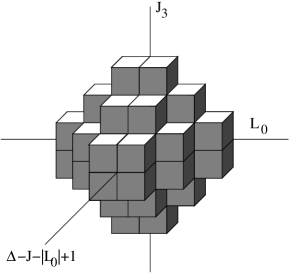
Figure 2: A graphical depiction of the $\Delta=5/2$ representation in $d=4$ with 40 states. The states are organized with respect to their $L_{0}$ eigenvalue, their $J_{3}$ eigenvalue, and their total spin $J$. Both $L_{0}$ and $J_{3}$ take half integer values between $-\Delta$ and $\Delta$, in this case $-5/2$ and $5/2$. The total spin $J$ goes from $1/2$ till $\Delta=5/2$. We plot $\Delta-J-|L_{0}|+1$ instead of $J$ since this gives a clearer picture. From the diagram it is obvious how to extend it to representations with other values of $\Delta$

As before, $L_{i-}$ annihilates $1$, the highest weight state, so the representation is bounded from below. The algebra has finite representations if it is also bounded from above i.e. if the lowest weight state is annihilated by $L_{i+}$. For a given $\Delta$, we find that

$$L_{i+}(x^{2})^{\Delta-1/2}x\!\cdot\!\gamma=0\;,$$ (34)

where $x\!\cdot\!\gamma$ stands for $x_{i}\gamma^{i}$. Hence we should take representations with half-integer conformal dimension. The monomials again form an eigenbasis for $L_{0}$. For example, we have

$$\Delta=1/2 : 1\;\;,\,\;x\!\cdot\!\gamma\;$$

$$\Delta=3/2 : 1\;\;,\,\;x_{i}\;\;,\,\;x_{i}\,x\!\cdot\!\gamma\;\;,\,\;x^{2}\,x\!\cdot\!\gamma$$

$$\Delta=5/2 : 1\;\;,\,\;x_{i}\;\;,\,\;x_{i}x_{j}\;\;,\,\;x_{i}x_{j}\,x\!\cdot\!\gamma\;\;,\,\;x^{2}\,x_{i}x\!\cdot\!\gamma\;\;,\,\;x^{4}\,x\!\cdot\!\gamma\;.$$ (35)

Each monomial has an $O(d-1)$ spinor index as well. For example, when $d=4$, these are the ${\bf 4}$, the ${\bf 16}$, and the ${\bf 40}$ of $O(1,4)$ because each monomial comes with a two-component spinor. In figure 2 we have depicted the representation with 40 states.

In general, the rule is to take symmetric spinor-valued monomials up to order $\Delta-1/2$ as well as their duals under

$$\psi_{a}(x)\to\psi_{a}^{\prime}(x^{\prime})=(x^{2})^{\Delta-1/2}x\!\cdot\!\gamma^{b}_{a}\psi_{b}(x^{\prime})\;,$$ (36)

where ${x_{i}}^{\prime}=+x_{i}/x^{2}$ and $a,b$ are spinor indices. We see from (35) that the global Hilbert space now always splits into two subspaces which are dual to each other under (36). This map is an inversion around the equator. The pure monomial (i.e. not involving $x\!\cdot\!\gamma$) with high degree are concentrated closer to the horizon. We interpret therefore the pure monomials with highest degree and their mirror images with a factor $x\!\cdot\!\gamma$ as the states near the horizon. As we will discuss, the number of these states also grow as the area of the horizon.

To find the coordinate representations of an orthonormal basis for an observer’s Hilbert space, we should again diagonalize the $L_{0}$ eigenbasis, (35), with respect to the Cartan subalgebra of $so(d-1)$ and its Casimir. The latter is now

$$J^{2}=L^{2}+x\cdot\partial-x\!\cdot\!\gamma~{}\gamma\!\cdot\!\partial+{1\over 8}(d-1)(d-2)\;,$$ (37)

which one can check reduces to $(L+S)^{2}$ for $d=4$. In $d=4$, one can use the eigenfunctions of $L_{3}$ and $L^{2}$ from the previous subsection to construct eigenfunctions of $L_{0}$, $J_{3}$, and $J^{2}$. Denoting the coordinate representation of $|h\,j\,m_{j}\rangle$ as $\psi_{h,j,m_{j}}$, a short exercise in computing Clebsch-Gordan coefficients gives, for example:

$$\psi_{\Delta,\frac{1}{2},\frac{1}{2}}(x)=N_{1/2}\left(\begin{array}[]{cc}1\\ 0\end{array}\right)\;\;,\,\;\psi_{\Delta,\frac{1}{2},-\frac{1}{2}}(x)=N_{1/2}\left(\begin{array}[]{cc}0\\ 1\end{array}\right)\;,$$ (38)

which both have $L_{0}$ eigenvalue $+\Delta$ and $J^{2}$ eigenvalue 3/4, and

$$\psi_{\Delta-1,\frac{3}{2},\frac{3}{2}}(x)=N_{3/2}\left(\begin{array}[]{cc}{1\over\sqrt{2}}(x_{1}+ix_{2})\\ 0\end{array}\right)\;\;,\,\;\psi_{\Delta-1,\frac{3}{2},\frac{1}{2}}(x)=N_{3/2}\left(\begin{array}[]{cc}-\sqrt{2}x_{3}\\ {1\over\sqrt{2}}(x_{1}+ix_{2})\end{array}\right)$$ (43)

$$\psi_{\Delta-1,\frac{3}{2},-\frac{1}{2}}(x)=N_{3/2}\left(\begin{array}[]{cc}-{1\over\sqrt{2}}(x_{1}-ix_{2})\\ -\sqrt{2}x_{3}\end{array}\right)\;\;,\,\;\psi_{\Delta-1,\frac{3}{2},-\frac{3}{2}}(x)=N_{3/2}\left(\begin{array}[]{cc}0\\ {1\over\sqrt{2}}(x_{1}-ix_{2})\end{array}\right)\;,$$ (48)

which both have $L_{0}$ eigenvalue $+\Delta-1$ and $J^{2}$ eigenvalue 15/4.

A positive-definite hermitian inner product for the spinor fields is

$$(\psi_{m},\psi_{n})=\int{d^{d-1}x\over(1+x^{2})^{d-3/2+\Delta}}\left(\psi^{*}_{m}(x)x\!\cdot\!\gamma\psi^{\prime}_{n}(x^{\prime})+\psi_{n}(x)x\!\cdot\!\gamma^{*}\psi^{{}^{\prime}*}_{m}(x^{\prime})\right)\;.$$ (49)

This inner product is $O(d-1)$-invariant.

5.1 Counting of states and the large representation limit

To find the size of these representations, we need to count the number of symmetric monomials as well as the coordinates with $x\!\cdot\!\gamma$. In addition, there is a spinor index attached to everything. So for example, when $d=4$, there are 4 global Hilbert states at $\Delta=1/2$, 16 at $\Delta=3/2$, and 40 at $\Delta=5/2$ etc. Note that the $\Delta=1/2$ representation is just the spinor representation of the previous subsection, the four states corresponding to spin-up and spin-down for either antipodal observer. The antipodal states can be viewed as being created by spinor fields acting at $1$ and at its inverse, $(x^{2})^{\Delta}\,x\!\cdot\!\gamma$. The dimension of the global Hilbert space in representation $\Delta$ for $d$ even is

$${\rm dim}~{}h_{\Delta}=2\cdot 2^{(d-2)/2}\sum_{p=0}^{\Delta-1/2}\left(\begin{array}[]{c}d+p-2\\ p\end{array}\right)=2^{d/2}\left(\begin{array}[]{c}d+\Delta-3/2\\ \Delta-1/2\end{array}\right)\;.$$ (50)

For odd $d$, we just replace $2^{(d-2)/2}$ with $2^{(d-1)/2}$.

The global Hilbert states are labeled by an $O(1,d)$ index coming from the spinor, as well as an $O(1,d)$ index coming from the coordinates. This leads to a further decomposition as, for example,

$${\bf 4}\otimes{\bf 14}={\bf 40}\oplus{\bf 16}\;,$$ (51)

so an $O(1,4)$ spinor (the 4) on the 14 coordinates of (25) is reducible into a $\Delta=3/2$ and a $\Delta=5/2$ representation. Again the fact that these representations are finite is indicative of an underlying exclusion principle. We have essentially discretized the sphere. Indeed, some of the expressions are reminiscent of quantum foam [18].

Consider now what happens as the cosmological constant is decreased. As the horizon area increases, the number of states also increases so we are going towards larger representations. But now the size of the finite conformal representation on the sphere is related to the radius of the sphere itself (which is a Casimir of the representation). We see from (50), that the dimension of the tensor product space is

$$\ln{\rm dim}~{}H_{\Delta}=\left({\rm dim}~{}h_{\Delta}\right)\ln 2=\left[2^{d/2}\left(\begin{array}[]{c}N+d-1\\ N\end{array}\right)\right]\ln 2\;,$$ (52)

where $N=\Delta-1/2$ and $d$ has been taken to be even. The logarithm of the number of states in the Fock space therefore grows as

$${1\over 2}\ln{\rm dim}~{}H\sim N^{d-1}\;.$$ (53)

We see that the logarithm of the number of Fock states scales as the volume of the boundary sphere. These are states that live in one hemisphere of the boundary sphere. We can obtain an answer that scales as the area, by considering only those states that are entangled with states in the other hemisphere, i.e. with the states of the antipodal observer. These are the states at the equator of the sphere:

$$S=\left[2^{d/2}\left(\begin{array}[]{c}N+d-2\\ N\end{array}\right)\right]\ln 2\sim N^{d-2}\;.$$ (54)

Hence our construction seems to suggest that the entropy of de Sitter space counts the number of states entangled across the horizon [19].

Another interesting issue is the restoration of unitarity. The tensor product states form finite-dimensional representations of $O(1,d)$. Obviously, these representations are nonunitary. We can write a global Hilbert state as

$$\Psi=\psi(x)+\psi^{\prime}(x^{\prime})=\psi(x)+x\!\cdot\!\gamma(x^{2})^{\Delta-1/2}\psi(x^{\prime})\;.$$ (55)

Then an $O(1,d)$-invariant hermitian bilinear is

$$(\Psi_{1},\Psi_{2})=\int{d^{d-1}x\over(1+x^{2})^{d-1+\Delta}}\Psi^{\dagger}_{1}(x)\Gamma^{0}\Psi^{\prime}_{2}(x)\;.$$ (56)

This does not qualify as an inner product since it is not positive-definite; half the states have negative norm. Indeed, if one thinks of $h_{I}$ as being the electron Hilbert space and $h_{II}$ as being a positron Hilbert space, then $\overline{\Psi}\Psi$ is just $(e^{\dagger}e-p^{\dagger}p)$. From the inner product, and the way the generators act, it is clear that the nonunitarity of the representations is associated with the existence of the other side of the horizon. Furthermore, the construction is symmetric under the exchange of positive and negative norm states, very much like the symmetry between negative and positive energy states for Dirac spinors. This suggests that we should try to take the analogy further and “fill” the other side of the horizon like a Dirac sea. This leads to the appealing picture that the horizon becomes identified with a Fermi surface, an idea that has started to appear in other contexts as well. Furthermore, the states right at the surface grow precisely as the area of the horizon.

Consider now the generators $L_{i\pm}$. These generators can mix states of different observers by moving monomials across the equator. On the complete Fock space this action is nonunitary, since a positive norm state for one observer is in general a mixture of positive and negative norm states for another. But note that only those states that are already at the equator are moved into the antipodal observer’s states. States at other positions are merely moved closer or farther from the equator; on these states, the operators $L_{i\pm}$ are hermitian. For a given $N$, the ratio of equatorial states to total states falls as $1/N$. So, for very large representations, the conformal generators act in an increasingly unitary manner on states that belong to a single observer’s Fock space. In the Minkowski limit of an infinitely large representation, the generators become precisely unitary. Each Fock space then furnishes a unitary infinite-dimensional representation of the Poincaré group, and the two Fock spaces of the pair of antipodal observers decouple. The vanishing cosmological constant limit of de Sitter space is thus two copies of Minkowski space.

6 De Sitter-Invariance and the S-matrix

The spinor fields on the sphere give an infinite class of finite-dimensional nonunitary representations of the de Sitter group, all of which can be written as $h_{I}\oplus h_{II}$, with $h_{I}$ and $h_{II}$ both being unitary representations of the rotation group. We interpret these as the one-particle Hilbert space for a given observer. The Fock spaces $H_{I}$ and $H_{II}$ can thus be constructed as being two isomorphic but otherwise independent spaces. As described, these Hilbert space are representations of the little group that leave the horizon invariant. One can think of the corresponding charges as being defined at the horizon (note that, when going to the Minkowski space limit it becomes asymptotic infinity). In global de Sitter space there is no boundary, and hence no conserved charges. Therefore global states correspond to de Sitter-invariant tensor product states.

Observer complementarity states that each observer has complete but complementary information. The global states in de Sitter space do not give complete information to single observers, since they are described as entangled states. We can implement observer complementarity by making use of an antipodal map. As we will see, if we regard $H_{I}$ as the space of in-states, the antipodal identification takes $H_{II}$ and identifies it with the space of out-states. Furthermore, the de Sitter-invariant global state becomes the S-matrix that maps in-states to out-states. De Sitter invariance of the S-matrix is very natural: just as in Minkowski space, we want the S-matrix to respect the spacetime isometry group.

6.1 Antipodal map

The elliptic interpretation of de Sitter space [20, 6, 21, 22] consists of identifying events that are related by an involution, the $\mathbb{Z}_{2}$ antipodal map

$$X^{I}\to-X^{I}\;,$$ (57)

where $I=0,1,\ldots,D$, together with charge conjugation, C [6]. Here $X^{I}$ are the Cartesian embedding coordinates of $d+1$-dimensional Minkowski space; see (1). The fixed point of this identification, $X^{I}=0$ is not itself on the de Sitter hyperboloid, so this is a freely-acting symmetry. The quotient space, $dS/\mathbb{Z}_{2}$ or “elliptic de Sitter space,” is therefore a homogeneous space with no special points. Moreover, the transformation $X^{I}\to-X^{I}$ is in the center of the de Sitter group so the quotient space still has the same local symmetries and the question of finding finite-dimensional representations of the de Sitter group continues to apply. For a local observer, the geometry is unchanged but antipodal points on the horizon are identified. Indeed, if we think of de Sitter space as the Lorentzian version of a sphere, then elliptic de Sitter space is the Lorentzian version of a projective sphere.

Note that the antipodal map also inverts the direction of time; see Figure 3. As a result, elliptic de Sitter space is not time-orientable; there is no globally-consistent way to distinguish future light cones from past light cones.

Figure 3: The antipodal map reverses the local arrow of time.

For example, consider global coordinates. The line element reads

$$ds^{2}=-dT^{2}+R^{2}\cosh^{2}(T/R)\left(d\theta^{2}+\sin^{2}\theta~{}d\Omega^{2}_{D-2}\right)\;.$$ (58)

In these coordinates the antipodal map is given by

$$T\to-T\qquad\theta\to\pi-\theta\qquad\Omega\to\Omega^{A}\;,$$ (59)

where $\Omega^{A}$ are the angular coordinates of the point antipodal on the $D-2$-dimensional sphere to the point labeled by $\Omega$, and time is reversed, $T\to-T$. One can check that these identifications, even though they involve time, do not lead to any obvious inconsistencies involving causality [20, 6] such as closed timelike curves. There are several interesting consequences of making such an identification. Since the spacetime has effectively been halved by the $\mathbb{Z}_{2}$ identification, every observer now has complete information, in the sense that there are no independent events outside his or her horizon. Moreover, the global spacetime now has only one asymptotic boundary, rather than two, since $\mathcal{I}^{+}$ and $\mathcal{I}^{-}$ have been identified. This seems holographically more appealing since otherwise the dual theory would live on two disconnected manifolds.

Now the arrow of time in the antipodal observer’s causal patch points in the opposite sense. This suggests that if an observer’s space can be thought of as the space of initial states, then the antipodal Fock space should be regarded as the final state space [6, 23]. The tensor product states $|m\rangle_{I}\otimes|n\rangle_{II}$ should now be thought of as a physical process $|m\rangle_{\rm in}\otimes|n^{\prime}\rangle_{\rm final}$ where the prime indicates that the final state is a CPT conjugate of the corresponding ket e.g. $|\!\uparrow\rangle^{\prime}=|\!\downarrow\rangle$. We also have a choice, whether to map $|0\rangle_{\rm in}$ to $\langle 0|_{\rm out}$ or to $\langle\,\uparrow\downarrow\!|_{\rm out}$. Then taking the hermitian conjugate of (9), we find

$$\Psi=\sum_{m,n}C^{*}_{mn}|n^{\prime}\rangle_{\rm out}\otimes\langle m|_{\rm in}\;,$$ (60)

and hence $C^{\dagger}$ is just the S-matrix. The invariant tensor product states (63) are then the de Sitter-invariant building blocks of the S-matrix.

6.2 An illustration in terms of spinors

As an illustration let us find the invariant tensor product for the Dirac spinor construction in $d=4$; the same arguments will hold for the more general representations corresponding to the spinor field on the sphere. Our one-particle Hilbert space is therefore just $|\!\uparrow\rangle$ and $|\!\downarrow\rangle$; the Fock space is spanned by the four states $|0\rangle$, $|\!\uparrow\rangle$, $|\!\downarrow\rangle$, and $|\!\uparrow\downarrow\rangle$. These four states can be labeled by their transformation properties under $O(3)$. Obviously, they belong to the $\bf{1}$, the $\bf{2}$, and the $\bf{1}$ representations, respectively.

The antipodal observer has an isomorphic Fock space. The tensor product states therefore transform under the direct product of the respective representations. Taking the direct product of the $\bf{1}$, the $\bf{2}$, and the $\bf{1}$ with themselves we find that the 16 tensor product states belong to

$${\bf 1}\oplus{\bf 2}\oplus{\bf 1}\oplus{\bf 2}\oplus{\bf 3}\oplus{\bf 1}\oplus{\bf 2}\oplus{\bf 1}\oplus{\bf 2}\oplus{\bf 1}\;.$$ (61)

These are $O(3)$ labels. We are interested in how the tensor product states transform not just under rotations, but under general de Sitter transformations. We can “recompose” the above $O(3)$ representations into $O(1,4)$ representations:

$${\bf 1}\oplus{\bf 4}\oplus{\bf 5}\oplus{\bf 1}\oplus{\bf 4}\oplus{\bf 1}\;.$$ (62)

For example, the states $|0\rangle_{I}\otimes|\!\uparrow\rangle_{II}$, $|0\rangle_{I}\otimes|\!\downarrow\rangle_{II}$, $|\!\uparrow\rangle_{I}\otimes|0\rangle_{II}$, and $|\!\downarrow\rangle\otimes|0\rangle_{II}$ combine to form a $\bf{4}$, a spinor of $O(1,4)$. The $\bf{5}$ is a vector of $O(1,4)$.

Notice, in particular, that there are three singlet states. These are tensor product states that are invariant under the action of the de Sitter group. The three invariant states are

$$|0\rangle\otimes|0\rangle\qquad|\!\uparrow\downarrow\rangle\otimes|\!\uparrow\downarrow\rangle\qquad\left(|\!\uparrow\rangle\otimes|\!\downarrow\rangle-|\!\downarrow\rangle\otimes|\!\uparrow\rangle\right)\;.$$ (63)

As we have discussed, under the antipodal identification, tensor product states correspond to physical processes: the states in Fock space $I$ are initial states while the states in Fock space $II$ become final states. There are therefore three de Sitter-invariant processes in this simple model.

With $|0\rangle_{\rm in}\to\langle\,\uparrow\downarrow\!|_{\rm out}$, and with the rows and columns labeled in the order $|0\rangle$, $|\!\uparrow\rangle$, $|\!\downarrow\rangle$, $|\!\uparrow\downarrow\rangle$, a de Sitter-invariant S-matrix is

$$S=\left(\begin{array}[]{lc}0\;\;\;0\;\;\;0\;\;\,a\\ 0\;\;\;b\;\;\;0\;\;\;0\\ 0\;\;\;0\,\;\;b\;\;\;0\\ c\;\;\;0\;\;\;0\;\;\;0\end{array}\right)\;,$$ (64)

where we have used $T|\!\uparrow\rangle=\eta|\!\downarrow\rangle$ and $T|\!\downarrow\rangle=-\eta|\!\uparrow\rangle$ for time-reversal on spinors. If $a$, $b$, and $c$ are all phases, then the S-matrix is unitary as well as de Sitter-invariant. We learn that the number of independent S-matrix elements is the number of invariant tensor product states.

More generally, we can consider a Fock space that is the product of $N$ different Fock spaces, each the Fock space of a different species of spinor. One may think of $N$ as being the number of flavors. A basis state for this multi-species Fock space is

$$|\chi\rangle_{1}\otimes|\chi\rangle_{2}\otimes\ldots\otimes|\chi\rangle_{N}\;,$$ (65)

where each $|\chi\rangle$ can be $|0\rangle$, $|\!\uparrow\rangle$, $|\!\downarrow\rangle$, or $|\!\uparrow\downarrow\rangle$. For $N$ spinors there are $4^{N}$ Fock states and $4^{2N}$ tensor product states. Consider for example $N=2$. An individual observer’s Fock space is now itself a direct product of the Fock spaces of the two spinors. The $O(1,4)$ labels for the representations that the 16 Fock space states transform under are given precisely by (62). The same set of representations applies to the antipodal observer’s Fock space. There are then 256 tensor product states describing global de Sitter space. They are grouped in representations according to the direct product of $O(1,4)$ representations. We use the fact that

$${\bf 4}\otimes{\bf 4} = {\bf 10}\oplus{\bf 5}\oplus{\bf 1}$$

$${\bf 4}\otimes{\bf 5} = {\bf 16}\oplus{\bf 4}$$

$${\bf 5}\otimes{\bf 5} = {\bf 14}\oplus{\bf 10}\oplus{\bf 1}\;.$$ (66)

Hence the 256 tensor product states transform under

$$14\times{\bf 1}\oplus 16\times{\bf 4}\oplus 10\times{\bf 5}\oplus 5\times{\bf 10}\oplus 4\times{\bf 16}\oplus 1\times{\bf 14}\;.$$ (67)

Here there are 14 de Sitter-invariant tensor product states. This means that a de Sitter-invariant S-matrix can at most depend on 14 independent parameters.

Just as an aside, we note that the ${\bf 1}$, ${\bf 4}$, ${\bf 5}$, ${\bf 10}$, ${\bf 16}$, and the ${\bf 14}$ have a familiar interpretation if we regard $O(1,4)$ as the Lorentz group in five dimensions: in this language they represent the scalar, spinor, vector, antisymmetric tensor, gravitino, and graviton, respectively and form the ${\cal N}=2$ supergravity multiplet. This is perhaps not surprising since we built the representation out of two independent spinors. Notice further that the multiplicities are themselves the size of representations of a five-dimensional orthogonal group, which reflects the fact that in this toy example the symmetry group is actually $SO(5)\times SO(1,4)$.

The number of de Sitter invariants is in general much less than the number of conditions imposed by unitarity: in our example there are 256 S-matrix elements but only 14 invariants. In order for the S-matrix to be unitary, these 14 complex parameters have to be chosen to satisfy the 128 complex equations imposed by unitarity. The requirements of de Sitter symmetry and unitarity are therefore very constraining. One may worry that there may not be any solution but, as one can explicitly check, it is possible to satisfy de Sitter invariance and unitarity and still have a small but nonzero set of free parameters. This check has been preformed for small representations, and works remarkably. We do not have a general proof, but we regard the fact that is works in these case as an indication that at least in principle their is no clash between de Sitter invariance and unitarity. In fact, by considering larger representations and allowing several spinor fields we expect that it even becomes easier to obey both requirements. Finally, we note that gauge invariance can also be included in our construction by giving the spinor fields an extra representation index and requiring that the initial and final states are gauge invariant.

7 Observer Complementarity

We have argued that, after making the antipodal identification, every observer has complete information, and tensor product states become processes. However, the physical interpretation of these processes generally depends on the observer. This is a manifestation of what we call “observer complementarity,” the notion that each observer can, in principle, describe everything that happens within his or her horizon using only pure states. The physics however may appear in rather different – complementary – guises.

Our construction gives a realization of this notion of observer complementarity, not just in terms of pictures or words, but in the actual expressions. Consider the simplest case of one spinor in $d=4$. We saw that there were only three de Sitter-invariant states, (63). For example, the process

$$\left\{|\!\uparrow\rangle\to|\!\downarrow\rangle\right\}-\left\{|\!\downarrow\rangle\to|\!\uparrow\rangle\right\}$$ (68)

corresponds to a spin-flip, and all observers can agree on that. In contrast, spin-up going to spin-down is not a process that all observers agree on because

$$|\!\uparrow\rangle\to|\!\downarrow\rangle={1\over 2}\left(\left\{|\!\uparrow\rangle\to|\!\downarrow\rangle\right\}-\left\{|\!\downarrow\rangle\to|\!\uparrow\rangle\right\}\right)+{1\over 2}\left(\left\{|\!\uparrow\rangle\to|\!\downarrow\rangle\right\}+\left\{|\!\downarrow\rangle\to|\!\uparrow\rangle\right\}\right)\;,$$ (69)

and only the first term in parentheses transforms in the singlet; the second term transforms in the ${\bf 5}$ of $O(1,4)$.

More generally, the S-matrix contains the probability amplitudes for all possible events or processes. Every event is visible to all observers. But different observers give different interpretations of the same event in terms of a scattering process of in- to out-states. This is because the de Sitter group element that relates two observers mixes up the in- and out-states. At first this may seem to be in conflict with de Sitter invariance, but it is not. De Sitter invariance implies only that the probability amplitudes that each observer associates with the observed event are the same. The physical interpretation of the event as a scattering process may well be different. This is just like in Minkowski space, where generally in- and out-states do transform under the Lorentz group (though of course they do not mix), but may be expressed in terms of Lorentz-invariant “form factors.” In this sense, the number of de Sitter-invariant tensor products counts how many form factors can appear in the most general scattering process.

Acknowledgments

We like to thank Bartomeu Fiol, Lenny Susskind and Herman Verlinde for discussions. M. P. is a Columbia University Frontiers of Science fellow and is supported in part by DOE grant DF-FCO2-94ER40818.

References

- [1] A. Strominger, “The dS/CFT Correspondence,” JHEP 0110 (2001) 034; hep-th/0106113.
- [2] T. Banks, “Cosmological Breaking Of Supersymmetry, or Little Lambda Goes Back To The Future II,” hep-th/0007146.
- [3] W. Fischler, Talk at the 60th birthday of G. West, June 2000.
- [4] N. Goheer, M. Kleban, and L. Susskind, “The Trouble with de Sitter Space,” JHEP 0307 (2003) 056; hep-th/0212209.
- [5] E. Witten, “Quantum Gravity in de Sitter Space,” hep-ph/0106109.
- [6] M. Parikh, I. Savonije, and E. Verlinde, “Elliptic de Sitter Space: dS/,” Phys. Rev. D 67 (2003) 064005; hep-th/0209120.
- [7] L. Susskind, L. Thorlacius, and J. Uglum, “The Stretched Horizon and Black Hole Complementarity,” Phys. Rev. D 48 (1993) 3743; hep-th/9306069.
- [8] C.R. Stephens, G. ’t Hooft, and B. F. Whiting. “Black Hole Evaporation Without Information Loss,” Class. Quant. Grav. 11 (1994) 621; gr-qc/9310006.
- [9] Y. Kiem, E. Verlinde, and H. Verlinde, “Black Hole Horizons and Complementarity,” Phys. Rev. D 52 (1995) 7053; hep-th/9502074.
- [10] M. Parikh and E. Verlinde, “De Sitter Space With Finitely Many States: A Toy Story,” hep-th/0403140.
- [11] A. Guijosa and D. Lowe, “A New Twist on dS/CFT,” Phys. Rev. D 69 (2004) 106008; hep-th/0312282.
- [12] D. A. Lowe, “q-Deformed de Sitter/Conformal Field Theory Correspondence,” hep-th/0407188.
- [13] M. Spradlin, A. Strominger, and A. Volovich, “Les Houches Lectures on de Sitter Space,” hep-th/0110007.
- [14] D. Klemm and L. Vanzo, “Aspects of Quantum Gravity in de Sitter Spaces,” hep-th/0407255.
- [15] J. M. Maldacena and A. Strominger, “AdS(3) Black Holes and a Stringy Exclusion Principle,” JHEP 9812 (1998) 005; hep-th/9804085.
- [16] T. Banks, “Some Thoughts on the Quantum Theory of de Sitter Space,” astro-ph/0305037.
- [17] M. Li, “Matrix Model for de Sitter,” JHEP 0204 (2002) 005; hep-th/0106184.
- [18] A. Iqbal, N. Nekrasov, A. Okounkov, and C. Vafa, “Quantum Foam and Topological Strings,” hep-th/0312022.
- [19] D. Kabat and G. Lifshytz, “De Sitter Entropy from Conformal Field Theory,” JHEP 0204 (2002) 019; hep-th/0203083.
- [20] E. Schrödinger, “Expanding Universes,” Cambridge University Press, 1956.
- [21] G. Gibbons, “The Elliptic Interpretation of Black Holes and Quantum Mechanics,” Nucl. Phys. B271 (1986) 497.
- [22] N. Sanchez, “Quantum Field Theory and the ‘Elliptic Interpretation’ of de Sitter Space-Time,” Nucl. Phys. B294 (1987) 1111.
- [23] G. ’t Hooft, “On the Quantum Structure of a Black Hole,” Nucl. Phys. B256 (1985) 727.