Spiky strings and single trace operators in gauge theories

Abstract:

We consider single trace operators of the form $\mathcal{O}_{l_{1}\ldots l_{n}}=\mbox{Tr}D_{+}^{l_{1}}F\ldots D_{+}^{l_{n}}F$ which are common to all gauge theories. We argue that, when all $l_{i}$ are equal and large, they have a dual description as strings with cusps, or spikes, one for each field $F$. In the case of $\mathcal{N}=4$ SYM, we compute the energy as a function of angular momentum by finding the corresponding solutions in $AdS_{5}$ and compare with a 1-loop calculation of the anomalous dimension. As in the case of two spikes (twist two operators), there is agreement in the functional form but not in the coupling constant dependence. After that, we analyze the system in more detail and find an effective classical mechanics describing the motion of the spikes. In the appropriate limit, it is the same (up to the coupling constant dependence) as the coherent state description of linear combinations of the operators $\mathcal{O}_{l_{1}\ldots l_{n}}$ such that all $l_{i}$ are equal on average. This agreement provides a map between the operators in the boundary and the position of the spikes in the bulk. We further suggest that moving the spikes in other directions should describe operators with derivatives other than $D_{+}$ indicating that these ideas are quite generic and should help in unraveling the string description of the large-N limit of gauge theories.

1 Introduction

It has since long been suspected that four dimensional confining theories have a dual string description, at least in the large-N limit [1]. The strings should emerge as the flux tubes of the confining force. However it was only relatively recently that a precise duality between a gauge theory and a string theory was established through the AdS/CFT correspondence [2]. It turned out however that the theory in question (${\cal N}=4$ SYM dual to $IIB$ strings on $AdS_{5}\times{S}^{5}$) is not confining and therefore another explanation for the appearance of strings was required. In a recent paper, Berenstein, Maldacena and Nastase [3] made the first steps in that direction by showing that certain operators in the boundary theory corresponded to string excitation in the bulk. After that, it was observed that such relation followed from a more general relation between that of semi-classical rotating strings in the bulk [4] and certain operators in the boundary. A lot of activity followed those papers. In particular many new rotating solutions were found. In a parallel development, Minahan and Zarembo [8] observed that the one-loop anomalous dimension of operators composed of scalars in ${\cal N}=4$ SYM theory follows from solving and integrable spin chain. This allowed the authors of [10] to make a much more detailed comparison between particular string solutions and certain operators in the gauge theory. This result followed from a detailed analysis of the dilatation operator which was discussed in [12, 13], rotating string solutions [14] and previous calculations [11]. Also, an important role in the comparison is taken by the study of the integrable structures of both sides of the correspondence [15, 16].

It was later suggested [17] that a classical sigma model action follows from considering the low energy excitations of the spin chain. It turned out that such action agrees with a particular limit of the sigma model action that describes the propagation of the strings in the bulk. This idea was extended to other sectors including fermions and open strings in [18, 19, 20, 21, 22, 23, 24, 25, 26, 27, 28] and to two loops in [29]. In [30, 31] the relation to the Bethe ansatz approach was clarified. Further, similar possibilities were found in certain subsectors of QCD [32]. An interesting summary on the relation between previous work in QCD and the more recent work can be found in [33]. A different but related approach to the relation between the string and Yang-Mills operators has been successfully pursued in [34, 35, 36] where a geometric description in terms of light like world-sheets was found. In that respect see also [37] and the discussion of supersymmetry in [38].

However, most of that work referred to a situation where the string was moving, at least partially on the sphere of $AdS_{5}\times{S}^{5}$. Nevertheless, solutions rotating purely on ${AdS}_{5}$ are known, an example being the folded rotating string of [4] which was conjectured to be dual to twist two operators in the gauge theory. This relation was confirmed in [39, 40] where it was shown that similar results for the anomalous dimension are obtained by using Wilson loops with cusps (following previous work in QCD [41]). Twist two operators are single trace operators of the form

$$\mathcal{O}=\mbox{Tr}\,\Phi_{1}\,({\stackrel{{\scriptstyle\leftrightarrow}}{{D}}}_{+})^{l}\ \Phi_{2}$$ (1.1)

where $D_{+}$ denotes the covariant derivative in a light-cone direction $x_{+}$ ($x_{+}=x+t$ in Minkowski and $x_{+}=x_{1}+ix_{2}$ in Euclidean signature) and $\Phi_{1}$, $\Phi_{2}$ indicate generic adjoint fields in the gauge theory. In QCD the anomalous dimension of these operators play an important role in the understanding of deep inelastic scattering [42].

In our case, we are interested in single trace operators because they are the relevant ones in the large-N limit of gauge theories and we would like to find a string description for them. The most generic single trace operator is of the form (suppressing Lorentz indices)

$$\mathcal{O}=\mbox{Tr}D^{l_{1}}\Phi_{1}\ldots D^{l_{n}}\Phi_{n}$$ (1.2)

that is, has an arbitrary number of fields $\Phi_{i}$ instead of just two, and the derivatives can be in any direction. As an intermediate step to the full understanding of these operators, in this paper we concentrate on the simpler case

$$\mathcal{O}=\mbox{Tr}D_{+}^{l_{1}}\Phi_{1}\ldots D_{+}^{l_{n}}\Phi_{n}$$ (1.3)

namely when all derivatives are along the same direction $x_{+}$. Moreover, we also consider that the number of derivatives is large ($l_{i}\gg 1$). In this limit the anomalous dimension is dominated by the contribution of the derivatives and we can ignore the exact nature of the fields $\Phi_{i}$ (in principle they do not even need to be elementary fields, they can also be composite fields of small conformal dimension). In the case of twist two operators, there is an associated string [4] (which is a closed string folded on itself to resemble a line segment) meaning that strings can be associated to such operators even when the number of fields is small. This appears different of what was discussed in [17] where it was shown that a sigma model/string action follows from taking a continuum limit when the number of operators is very large, each operator being associated to a portion of the string. However it is not actually different if we think of associating each portion of the string to each covariant derivative. In that case, the operators $\Phi_{i}$ should appear as distinguished points along the string. In the case of twist two operators there are two fields $\Phi_{1,2}$ and two distinguished points, namely the two cusps at the end points of the segment along which the string is folded. By analogy we expect that if we have $n$ operators, there should be $n$ distinguished points. One can, therefore, conjecture that operators of the form (1.3) have a dual description in terms of rotating strings with $n$ cusps as already suggested in [43]. We test this idea by considering such strings rotating in ${AdS}_{5}$ and comparing their energy with a 1-loop calculation in the field theory in the limit of large angular momentum $J$. The leading term in the anomalous dimension is $n/2$ times the result for the case of two cusps and behaves as $\ln J$. In the field theory the result is reproduced, up to the coupling constant dependence, by considering and operator with equal number of derivatives acting on each field. In particular, this again implies that the total number of derivatives, namely the angular momentum, is a multiple of $n$, the number of fields.

At the next order in $J$ which is order one, such operator is not an eigenstate of the dilatation operator. To better understand the system we map the operators into configurations of a spin chain with $n$ sites, one for each field, and with an infinite number of states per site, labeled by $l_{i}$ ($i=\ldots n$), the number of derivatives. We then consider a coherent state description derived in [22] and further studied in [22, 27, 30, 43] (following previous ideas in [8, 9, 12, 13, 43]). This description assumes that each site $i$ of the chain is in a coherent state parameterized by two variables $\rho_{i},\theta_{i}$. The average number of derivatives is $\langle l_{i}\rangle=\sinh^{2}(\rho_{i})$ which is consider to be constant. When $l_{1}\gg 1$, the action of the dilatation operator on these states can be described in terms of a classical action for the remaining variables $\theta_{i}$.

On the string side we consider the possibility that the spikes move, shifting their angular position and find an effective classical mechanics that describes this motion. Up to the coupling constant dependence it agrees with the one derived from the coherent state picture in the regime where the number of derivatives at each site is large (or equivalently the energy of each spike is large).

We should emphasize once more that this fact does not imply an agreement between string and gauge theory since the couplings are different on both sides. In spite of that, we believe that the comparison is still remarkable because it means that there is a string description of the operators even at 1-loop. The only point is that such string propagates in an ${AdS}_{5}$ space of different radius than at strong coupling.

The organization of this paper is as follows: in section §2 we study the solutions in flat space and in section §3 we extend them to AdS space, deriving also an effective description in terms of the dynamics of cusps. In section §4 we compare this description with the 1-loop field theory description of the dual operators and finally give our conclusions in section §5.

2 Spiky strings in flat space

As with the folded string, it is convenient to start by studying the solutions in flat space and then generalize them to AdS. This is so because in flat space the solutions are particularly simple and therefore all their properties can be easily derived. This simplicity is manifest in conformal gauge where they become just a superposition of a left and a right moving wave:

$$x = \lambda\,\cos\left((n-1)\ \sigma_{+}\right)+\lambda\,(n-1)\,\cos\left(\sigma_{-}\right)$$ (2.4)

$$y = \lambda\,\sin\left((n-1)\ \sigma_{+}\right)+\lambda\,(n-1)\,\sin\left(\sigma_{-}\right)$$ (2.5)

$$t = 2\,\lambda\,(n-1)\,\tau=\lambda\,(n-1)\,(\sigma_{+}+\sigma_{-})$$ (2.6)

where $\sigma_{+}=\tau+\sigma$, $\sigma_{-}=\tau-\sigma$, $n$ is an integer and $\lambda$ is constant that determines the size of the string. Here, ($\tau,\sigma$) parameterize the world-sheet of a string moving in a Minkowski space of metric:

$$ds^{2}=-dt^{2}+dx^{2}+dy^{2}$$ (2.7)

The solutions are periodic in $\sigma$ with period $2\pi$ and satisfy the equations of motion in conformal gauge:

$$(\partial_{\tau}^{2}-\partial_{\sigma}^{2})X^{\mu}=0,\ \ \ X^{\mu}=(t,x,y)$$ (2.8)

as well as the constraints

$$(\partial_{+}X)^{2}=(\partial_{-}X)^{2}=0$$ (2.9)

Quantum mechanically the state has $n_{R}=\lambda^{2}(n-1)^{2}$ right moving excitations of wave number $k_{R}=1$ and $n_{L}=\lambda^{2}(n-1)$ left moving excitations with wave number $k_{L}=n-1$ (satisfying the level matching condition $n_{R}k_{R}=n_{L}k_{L}$).

All excitations carry one unit of angular momentum and therefore the total angular momentum and energy are given by

$$J=n_{L}+n_{R}=\lambda^{2}n(n-1),\ \ E=\sqrt{2(n_{L}k_{L}+n_{R}k_{R})}=2\lambda(n-1),\ \ E=2\sqrt{\frac{n-1}{n}J}$$ (2.10)

which agrees with a classical computation. For $n=2$ we recover the standard Regge trajectory $E=\sqrt{2J}$ and for $n>2$ we get a Regge trajectory of modified slope. The variation in slope is not large since for $n\rightarrow\infty$ we get $E=2\sqrt{J}$ (however, this limit is singular because the string has infinite energy).

At fixed time, the shape of the string for different values of $n$ takes the form depicted in figs.(1) and (2). It can be seen that the string has $n$ spikes or cusps and, analyzing the time dependence, that it rotates rigidly in such a way that the end points of the spikes move at the speed of light. Notice that this does not necessarily mean that a point of fixed $\sigma$ moves in a circle since the string can slide on itself. In the appendix we introduce other world-sheet coordinates where $\sigma$ parameterizes the shape of the string and translations in $\tau$ correspond to rigid rotations. It is clear however that in such a gauge $\dot{X}.X^{\prime}\neq 0$ and therefore it is not the conformal gauge used in this section.

To find the position of the cusps we can use the fact they appear whenever $X^{\prime 2}=0$ which happens if

$$(n-1)\sigma_{+}-\sigma_{-}=2\pi m,\ \ \Rightarrow\ \ \sigma=2\pi\frac{m}{n}-\frac{n-2}{n}\tau\ \ \ \mbox{with}\ \ m=0\ldots n-1\ .$$ (2.11)

Therefore, there are $n$ cusps which, for $\tau=0$, are at $\sigma=2\pi\frac{m}{n}$, $m=0\ldots n-1$. In space time they are located at $r=r_{c}=n\lambda$ and $\theta=2\frac{n-1}{n}\tau-2\pi\frac{m}{n}$ where $(r,\theta)$ are standard polar coordinates in the plane $(x,y)$. The velocity at which the spikes move is given by

$$v=r_{c}\frac{d\theta}{dt}=r_{c}\frac{d\theta}{d\tau}\frac{d\tau}{dt}=1$$ (2.12)

namely, the speed of light.

As a final point, to which we will come back later, note that $J$ can be written as $J=n_{L}n$ and therefore is a multiple of $n$. The same result can be argued using the classical solution: since the shape of the string is invariant under rotations of $\frac{2\pi}{n}$, if we quantize it as a rigid body, the only allowed values of $J$ are multiples of $n$ in such a way that the wave function has the same symmetry under $\frac{2\pi}{n}$ rotations. More precisely, if $|\theta\rangle$ denotes a state where the configuration is rotated by an angle $\theta$, a state of angular momentum $J$ is

$$\mbox{$|J\rangle$}=\int_{0}^{2\pi}e^{iJ\theta}\mbox{$|\theta\rangle$}\,d\theta$$ (2.13)

If $\mbox{$|\theta\rangle$}=\mbox{$|\theta+\frac{2\pi}{n}\rangle$}$, the integral vanishes unless $J$ is a multiple of $n$.

The argument based on the shape of the classical solution becomes important in the ${AdS}_{5}$ case where we cannot quantize the string exactly.

In the next section we generalize these solutions to AdS space. Before doing that however let us comment in one counterintuitive feature of the flat space solutions. In the folded rotating string one argues that the tension of the string provides the centripetal force necessary for circular motion. The same idea applies for the spikes here but, on the other hand, the bottom of the valleys should be pulled outwards by the rest of the string, opposite to the centripetal acceleration. The first point to explain what happens is that there is no centripetal acceleration since the valley is instantaneously at rest as a simple calculation shows and as also follows from the fact that, at the bottom of the valley, any angular motion is parallel to the string and therefore unphysical. Nevertheless it is still true that the rest of the string pulls this point outwards in the radial direction. Again a simple computation reveals that the point moves away from the origin in such a way that it still stays on the string profile. Namely, the string rotates and therefore an instant later, at the same angular position, the radial position of the string increased exactly to match the outward motion of the portion of string at the valley.

Figure 1: Rotating string with 3 spikes in flat space. We plot $(x,y)$ in eq.(2.6) parametrically as a function of $\sigma=0\rightarrow 2\pi$ for $n=3$, $\lambda=1$ and $\tau=0$.

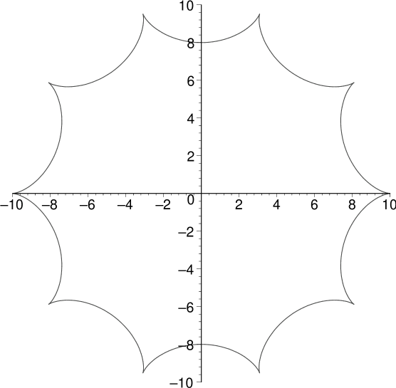
Figure 2: Rotating string with 10 spikes in flat space. We plot $(x,y)$ in eq.(2.6) parametrically as a function of $\sigma=0\rightarrow 2\pi$ for $n=10$, $\lambda=1$ and $\tau=0$.

Figure 3: Rotating string with 3 spikes in AdS space. In the figure, $(\rho,\theta)$ in eq.(3.14) are standard polar coordinates and we use the ansatz (3.15) together with (3.22) (and $\tau=0$) to plot one half of a spike and then rotate and reflect to plot the others. The same result can be obtained by using (3.33) which does not require this gluing procedure. In both cases the parameters are $\rho_{0}=0.2688735$, $\rho_{1}=2$.

Figure 4: Rotating string with 10 spikes in AdS space obtained in the same way as fig.3 but with $\rho_{0}=0.88266273$, $\rho_{1}=2$.

3 Spiky strings in AdS

For the case of string rotating in AdS we were not able to find such simple expressions as for the flat space case. We resort to using the Nambu-Goto action which leads to more complicated expressions but whose properties are still easily understood. Consider a string moving in a space parameterized by $(t,\rho,\theta)$ with metric

$$ds^{2}=-\cosh^{2}\!\rho\,dt^{2}+d\rho^{2}+\sinh^{2}\!\rho\,d\theta^{2}$$ (3.14)

which is the metric of ${AdS}_{3}$ which can be considered as embedded in ${AdS}_{5}$ for the purposes of the AdS/CFT correspondence. We choose world-sheet coordinates in such a way that

$$t=\tau,\ \ \theta=\omega\tau+\sigma,$$ (3.15)

and make the ansatz that the string is rigidly rotating which implies $\rho=\rho(\sigma)$, namely $\partial_{\tau}\rho=0$. The Nambu-Goto action is

$$S=-\frac{\sqrt{\lambda}}{2\pi}\int\sqrt{-\dot{X}^{2}{X^{\prime}}^{2}+(\dot{X}X^{\prime})^{2}}$$ (3.16)

where $\lambda$ is the ’t Hooft coupling in the field theory and the scalar products are taken with the metric (3.14). Notice that we set the radius $R$ of ${AdS}_{5}$ to one by writing explicitly the ’t Hooft coupling whenever $R^{2}/\alpha^{\prime}$ should have appeared. This makes all quantities adimensional. The ansatz we use implies that

$$\dot{X}^{2}=-\cosh^{2}\rho+\omega^{2}\sinh^{2}\rho,\ \ {X^{\prime}}^{2}={\rho^{\prime}}^{2}+\sinh^{2}\rho,\ \ \dot{X}X^{\prime}=\omega\sinh^{2}\rho$$ (3.17)

and

$$\sqrt{-\dot{X}^{2}{X^{\prime}}^{2}+(\dot{X}X^{\prime})^{2}}=\sqrt{{\rho^{\prime}}^{2}(\cosh^{2}\rho-\omega^{2}\sinh^{2}\rho)+\sinh^{2}\rho\cosh^{2}\rho}$$ (3.18)

We can further check that the equations of motion for $t$ and $\theta$, following from the action (3.16), are satisfied if

$$\rho^{\prime}=\frac{1}{2}\frac{\sinh 2\rho}{\sinh 2\rho_{0}}\frac{\sqrt{\sinh^{2}2\rho-\sinh^{2}2\rho_{0}}}{\sqrt{\cosh^{2}\rho-\omega^{2}\sinh^{2}\rho}}$$ (3.19)

where $\rho_{0}$ is an integration constant. Furthermore we can check that, if we assume (3.19), the equation of motion for $\rho$ is also satisfied. From the expression for $\rho^{\prime}$ we see that $\rho$ varies from a minimum value $\rho_{0}$ to a maximum value $\rho_{1}=\mbox{arccoth}\,\omega$. At $\rho=\rho_{1}$, $\rho^{\prime}$ diverges indicating the presence of a spike and at $\rho=\rho_{0}$ vanishes, indicating the bottom of the valley between spikes. To get a solution with $n$ spikes we should glue $2n$ of the arc segments we get here. For that we need to choose $\rho_{1}$ and $\rho_{0}$ in such a way that the angle between cusp and valley is $\frac{2\pi}{2n}$. This fixes one constant. The other, for example, can be fixed by giving the total angular momentum $J$. In that way we can determine the energy $E(n,J)$.

3.1 Exact solution

If we take equation (3.19) for $\rho$ and do the following change of variables:

$$u=\cosh 2\rho,\ \ \ u_{0}=\cos 2\rho_{0},\ \ \ u_{1}=\cosh 2\rho_{1}.$$ (3.20)

the resulting integral can be computed in terms of the elliptic function $\Pi$ defined as [44]

$$\Pi(\alpha,n,p)=\int_{0}^{\alpha}\frac{d\beta}{\sqrt{1-p^{2}\,\sin^{2}\!\!\beta}\ (1-n\,\sin^{2}\!\!\beta)},\ \ \ \ \alpha\leq\frac{\pi}{2}$$ (3.21)

The result is

$$\sigma = \frac{\sinh 2\rho_{0}}{\sqrt{2}\sqrt{u_{0}+u_{1}}\sinh\rho_{1}}\left\{\Pi(\alpha,\frac{u_{1}-u_{0}}{u_{1}-1},p)-\Pi(\alpha,\frac{u_{1}-u_{0}}{u_{1}+1},p)\right\}$$ (3.22)

where

$$p = \sqrt{\frac{u_{1}-u_{0}}{u_{1}+u_{0}}}$$ (3.23)

$$\sin\alpha = \sqrt{\frac{u_{1}-u}{u_{1}-u_{0}}}$$ (3.24)

The resulting shape, for constant time and two different values of $n$, is depicted in figs.(3) and (4). The angle difference between the spike and the valley as well as the angular momentum and energy carried by the string can be computed as

$$\Delta\theta = 2\int_{\rho_{0}}^{\rho_{1}}\frac{\sinh 2\rho_{0}}{\sinh 2\rho}\frac{\sqrt{\cosh^{2}\rho-\omega^{2}\sinh^{2}\rho}}{\sqrt{\sinh^{2}2\rho-\sinh^{2}2\rho_{0}}}\,d\rho$$ (3.25)

$$J = \frac{2n}{2\pi}\frac{\omega}{2}\sqrt{\lambda}\int_{\rho_{0}}^{\rho_{1}}\frac{\sinh\rho}{\cosh\rho}\frac{\sqrt{\sinh^{2}2\rho-\sinh^{2}2\rho_{0}}}{\sqrt{\cosh^{2}\rho-\omega^{2}\sinh^{2}\rho}}\,d\rho$$ (3.26)

$$E-\omega J = \frac{2n}{2\pi}\frac{1}{2}\sqrt{\lambda}\int_{\rho_{0}}^{\rho_{1}}\sinh 2\rho\frac{\sqrt{\cosh^{2}\rho-\omega^{2}\sinh^{2}\rho}}{\sqrt{\sinh^{2}2\rho-\sinh^{2}2\rho_{0}}}\,du$$ (3.27)

As discussed before, $\lambda$ is the ’t Hooft coupling, and $n$ the number of spikes which determines $\Delta\theta=\frac{2\pi}{2n}$. Note also that $E$ and $J$ are multiplied by $2n$ to obtain the total energy and angular momentum. Again, the change of variables (3.20) proves useful reducing the computation to elliptic integrals:

$$\Delta\theta = \frac{\sinh 2\!\rho_{0}}{\sqrt{2}\sinh\rho_{1}}\frac{1}{\sqrt{u_{1}-u_{0}}}\left\{\Pi(\frac{\pi}{2},\frac{u_{1}-u_{0}}{u_{1}-1},p)-\Pi(\frac{\pi}{2},\frac{u_{1}-u_{0}}{u_{1}+1},p)\right\}$$ (3.28)

$$J = \frac{2n}{2\pi}\ \frac{\sqrt{\lambda}}{\sqrt{2}}\ \frac{\cosh\rho_{1}}{\sqrt{u_{1}+u_{0}}}\ \bigg{\{}-(1+u_{0})\mathbf{K}(p)+(u_{1}+u_{0})\mathbf{E}(p)-$$ (3.29)

$$\ \ \ \ \ \ \ \ \frac{u^{2}_{0}-1}{u_{1}+1}\Pi(\frac{\pi}{2},\frac{u_{1}-u_{0}}{u_{1}+1},p)\bigg{\}}$$

$$E-\omega J = \sqrt{\lambda}\ \frac{2n}{2\pi}\ \frac{\sqrt{u_{1}+u_{0}}}{\sqrt{2}\sinh\rho_{1}}\ \left(\mathbf{K}(p)-\mathbf{E}(p)\right)$$ (3.30)

with $p$ as in (3.23). The functions $\mathbf{K(p)}$ and $\mathbf{E}(p)$ are defined by [44]:

$$\mathbf{K}(p)=\int_{0}^{\frac{\pi}{2}}\frac{d\alpha}{\sqrt{1-p^{2}\sin^{2}\alpha}},\ \ \ \mathbf{E}(p)=\int_{0}^{\frac{\pi}{2}}\sqrt{1-p^{2}\sin^{2}\alpha}\,d\alpha$$ (3.31)

Although it is interesting that the result can be expressed in terms of well-studied functions the actual expressions are not very illuminating and will not be used in the rest of the paper. For comparison with the field theory we consider now the limit in which the string is moving in such a way that $\rho_{1}\gg 1$ which, as we will see, is the large angular momentum limit. Before doing that however, we would like to clarify the process of gluing several segments to form the string. In the previous section that was not necessary and here actually it is not necessary either. It rather appears because of the choice of world-sheet coordinates. We can define a new $\tilde{\sigma}$ such that

$$\theta-\omega\tau=\sigma = \frac{\sinh 2\rho_{0}}{\sinh\rho_{1}\sqrt{2(u_{1}+u_{0})}}\left\{\int_{0}^{\tilde{\sigma}}\frac{d\alpha}{\sqrt{1-p^{2}\sin^{2}\alpha}\ [1-\frac{u_{1}-u_{0}}{u_{1}-1}\sin^{2}\alpha]}-\right.$$ (3.32)

$$\left.\int_{0}^{\tilde{\sigma}}\frac{d\alpha}{\sqrt{1-p^{2}\sin^{2}\alpha}\ [1-\frac{u_{1}-u_{0}}{u_{1}+1}\sin^{2}\alpha]}\right\}$$

$$\sinh^{2}\rho = \sinh^{2}\rho_{1}\cos^{2}\tilde{\sigma}+\sinh^{2}\rho_{0}\sin^{2}\tilde{\sigma}$$ (3.33)

The integrals are of the form (3.21) and then at first sight it seems that $\tilde{\sigma}$ is the same as $\alpha$ in (3.22). However care should be taken since this is valid only for the first half spike (at least according to the standard definition of the elliptic integral which is valid for $\alpha\leq\frac{\pi}{2}$). As defined here, $\sigma$ is a monotonically increasing function of $\tilde{\sigma}$, namely $\frac{d\sigma}{d\tilde{\sigma}}\geq 0$ with $\frac{d\sigma}{d\tilde{\sigma}}=0$ precisely at the cusps since $\frac{d\rho}{d\sigma}=\frac{d\rho}{d\tilde{\sigma}}\frac{d\tilde{\sigma}}{d\sigma}$ diverges if $\frac{d\sigma}{d\tilde{\sigma}}=0$. In fact, that is the only indication of the presence of cusps since now $\theta$ and $\rho$ are regular functions of $\tilde{\sigma}$ and no gluing process is needed. Of course, what we still need to do is to adjust $\rho_{0}$ and $\rho_{1}$ to get the right periodicity for $\theta(\tilde{\sigma})$ and $\rho(\tilde{\sigma})$.

3.2 Asymptotic expansion

To compare with the field theory we take a large angular momentum limit corresponding to $\rho_{1}\gg 1$. In this limit, the energy $E$ turns out to be equal, at leading order, to the angular momentum $J$ and the difference $E-J$, which we compare to the field theory, is proportional to $\sqrt{\lambda}(\rho_{1}-\rho_{0})$. In view of this, we require, in addition, that $\sqrt{\lambda}(\rho_{1}-\rho_{0})\gg 1$ which means that the spike carries a large energy and can be described semi-classically.

In this limit, $\omega=\coth\rho_{1}\rightarrow 1$, and a good approximation is obtained by replacing $\omega=1$ in $\Delta\theta$ and $E-\omega J$. This results in

$$E-J\simeq E-\omega J \simeq \frac{2n}{2\pi}\sqrt{\lambda}\int_{\rho_{0}}^{\rho_{1}}\!\!\!\frac{\sinh 2\rho}{\sqrt{\sinh^{2}2\rho-\sinh^{2}2\rho_{0}}}\,d\rho=\frac{2n}{4\pi}\sqrt{\lambda}\,\mbox{arccosh}\frac{u_{1}}{u_{0}}$$ (3.34)

$$\Delta\theta \simeq 2\int_{\rho_{0}}^{\rho_{1}}\frac{\sinh 2\rho_{0}}{\sinh 2\rho}\frac{d\rho}{\sqrt{\sinh^{2}2\rho-\sinh^{2}2\rho_{0}}}$$ (3.35)

(3.36)

$$= \frac{\pi}{4}-\frac{1}{2}\arcsin\left(\frac{1+u_{1}^{2}-2u_{1}^{2}/u_{0}^{2}}{u_{1}^{2}-1}\right)$$

where, as in (3.20) we defined $u_{1}=\cosh 2\rho_{1}$ and $u_{0}=\cosh 2\rho_{0}$. From here we obtain the energy of each half-spike as

$$\frac{E-J}{2n} \simeq \frac{\sqrt{\lambda}}{8\pi}\mbox{arccosh}\left(1+2\sinh^{2}2\rho_{1}\sin^{2}\Delta\theta\right)$$ (3.37)

$$\simeq \frac{\sqrt{\lambda}}{8\pi}\left\{4\rho_{1}+\ln(\sin^{2}\Delta\theta)\right\}$$ (3.38)

where the last approximation is done using $\rho_{1}\gg 1$ and assumes that $\Delta\theta$ is not as small as to make $e^{2\rho_{1}}\sin\Delta\theta\gg 1$ invalid. This means that we cannot put an extremely large number of operators $n\sim e^{2\rho_{1}}$. As shown below, this is equivalent to the assumption $\rho_{1}-\rho_{0}\gg 1$. The result (3.37) can also be derived easily in a more illuminating way. Indeed, the approximation $\omega\simeq 1$ can be done directly in the Nambu-Goto action resulting in

$$S_{NG} = -\frac{\sqrt{\lambda}}{2\pi}\int\sqrt{\rho^{\prime 2}(\cosh^{2}\rho-\omega^{2}\sinh^{2}\rho)+\sinh^{2}\rho\cosh^{2}\rho}$$ (3.39)

$$\simeq -\frac{\sqrt{\lambda}}{4\pi}\int\sqrt{(2\rho^{\prime})^{2}+\sinh^{2}2\rho}$$ (3.40)

This means that, in this limit, the action is simply the one for geodesics in the metric

$$ds^{2}=(d\tilde{\rho})^{2}+\sinh^{2}\!\tilde{\rho}\,d\theta^{2}$$ (3.41)

where $\tilde{\rho}=2\rho$, we parameterize the geodesic with $\theta=\sigma$, and solve for $\rho(\sigma)$. The energy is therefore

$$\frac{E-J}{2n}=\frac{\sqrt{\lambda}}{8\pi}L(\rho_{1},\Delta\theta)$$ (3.42)

where $L(\rho_{1},\Delta\theta)$ is the geodesic distance between two points at the same value of $\tilde{\rho}=2\rho_{1}$ and separated by an angle $2\Delta\theta$ (recalling that $\Delta\theta$ is the angle between a peak and a valley, and therefore half the angle between peaks). The geodesic length in the hyperboloid (3.41) can be easily computed and agrees with (3.37).

To compute $J$, we notice that the largest contribution comes from $\rho\sim\rho_{1}$ where the denominator inside the integral (3.26) is small. Again, assuming $\rho_{1}-\rho_{0}\gg 1$, we can make the approximation that $\rho\sim\rho_{1}\gg\rho_{0}$ leading to

$$J \simeq \frac{2n}{2\pi}\sqrt{\lambda}\int_{\rho_{0}}^{\rho_{1}}\!\!\!\frac{\sinh^{2}\rho}{\sqrt{\cosh^{2}\rho-\omega^{2}\sinh^{2}\rho}}\,d\rho\simeq\frac{2n}{2\pi}\frac{\sqrt{\lambda}}{4}e^{\rho_{1}}\int_{\rho_{0}}^{\rho_{1}}\!\!\!\frac{e^{2\rho}}{\sqrt{e^{2\rho_{1}}-e^{2\rho}}}\,d\rho$$ (3.43)

$$\simeq \frac{2n}{2\pi}\frac{\sqrt{\lambda}}{4}e^{2\rho_{1}}$$

Let us now consider the limit in which $\rho_{1}\rightarrow\infty$ keeping $\rho_{0}$ fixed and large. In this limit (3.36) implies that

$$\Delta\theta\simeq\frac{1}{u_{0}}\simeq 2\ e^{-2\rho_{0}}$$ (3.44)

and (3.43) implies that $J\rightarrow\infty$. Since the number of spikes $n$ is equal to $n=\pi/\Delta\theta$, the limit $\rho_{1}\rightarrow\infty$ keeping $\rho_{0}$ fixed and large is the limit of large angular momentum keeping the number of spikes fixed. In this limit we get, from (3.38) and for large $J$:

$$E\simeq J+\sqrt{\lambda}\ \frac{n}{2\pi}\,\ln\left(\frac{4\pi}{n}\frac{J}{\sqrt{\lambda}}\right),\ \ \ \ \ \ \ \ (J\rightarrow\infty)$$ (3.45)

which, for $n=2$ agrees with the result obtained in [4] and in [39, 40] using a different method.

3.3 Fluctuations

Certain fluctuations around the solution correspond to a change in the positions of the tip of the spikes along the circle $\rho=\rho_{1}$. The potential energy of interaction between spikes is given by the energy of the string hanging between them as computed in (3.38), where we should now keep the (subleading) term proportional to $\ln(\sin^{2}\Delta\theta)$ which contains the dependence on their relative position. A kinetic energy appears when the spikes move with respect to each other. Since the tip of the spike moves at the speed of light this can only happen if a spike moves up or down in $\rho$. For example if it goes up the angular velocity decreases but at the same time there is a cost in energy since the spike is longer. More precisely, if the spike shift upward to a position $\rho_{1}+\delta\rho$ the energy cost is

$$\delta(E-J)=2\ \frac{\sqrt{\lambda}}{2\pi}\ \delta\rho$$ (3.46)

since, at constant $\Delta\theta$, from (3.38) we get $E-J\simeq 2\,\frac{\sqrt{\lambda}}{2\pi}\rho_{1}$ (the extra factor of $2$ is because (3.38) corresponds to half a spike). At the same time the variation in angular velocity is

$$\delta\omega=\frac{d}{d\rho_{1}}\frac{\cosh\rho_{1}}{\sinh\rho_{1}}\ \delta\rho=-\frac{1}{\sinh^{2}\rho_{1}}\ \delta\rho$$ (3.47)

From here we obtain

$$\delta(E-J)=-\frac{\sqrt{\lambda}}{2\pi}\ 2\sinh^{2}\!\rho_{1}\,\delta\omega=\frac{\sqrt{\lambda}}{2\pi}\ (\cosh 2\rho_{1}-1)\ \dot{\theta}$$ (3.48)

where we call $\theta$ the displacement of the spike with respect to a reference position moving at constant angular velocity. $\delta(E-J)$ acts as the kinetic energy. Putting all together we expect the dynamics of the spikes to be described by an action

$$S=\frac{\sqrt{\lambda}}{2\pi}\int\!\!d\tau\sum_{j}(\cosh 2\rho_{1}-1)\ \dot{\theta_{j}}-\frac{\sqrt{\lambda}}{8\pi}\int\!\!d\tau\sum_{j}\left\{4\rho_{1}+\ln(\sin^{2}(\frac{\theta_{j+1}-\theta_{j}}{2}))\right\}$$ (3.49)

where $\theta_{j}$ denotes the angular position of each spike assumed to move around the circle $\rho=\rho_{1}$. In the following section we compare this action with the field theory result obtained in terms of coherent operators.

Before doing that, however, let us finish this section by noticing that, in principle, the spikes could be moving in any direction along the $S^{3}$ of ${AdS}_{5}$:

$$ds^{2}=-\cosh^{2}\!\rho\ dt^{2}+d\rho^{2}+\sinh^{2}\!\rho\ d\Omega_{[3]}^{3}$$ (3.50)

When all spikes are moving at small velocities with respect to each other this motion is again expected to be described by the same classical mechanics. If we go to embedding coordinates where ${AdS}_{5}$ is the manifold described by:

$$X_{1}^{2}+X_{2}^{2}+X_{3}^{2}+X_{4}^{2}-X_{0}^{2}-X_{-1}^{2}=-1$$ (3.51)

and we introduce complex coordinates $Z_{1}=X_{1}+iX_{2}$, $Z_{2}=X_{3}+X_{4}$, $W=X_{0}+iX_{-1}$, the solutions we described move in $Z_{1}$, $W$. Since the phase of $W$ should be identified with time, the spatial sections we are interested in can be described as a coset $SU(1,1)/U(1)$. If we include motion in $Z_{2}$ this should generalize to $SU(2,1)/U(1)$.

4 Gauge theory description

4.1 Field theory operators and coherent state description

Now we would like to describe the operators dual to these strings in the field theory. First, for a small number of spikes and for $\rho_{1}$, namely the radial position of the tip of the spikes, approaching the boundary, it seems that the corresponding state in the boundary theory is that of a set of particles moving at almost the speed of light. One particle for each spike. Therefore, using the operator state correspondence the related operator, at least in the free theory, should be

$$\mathcal{O}=\mbox{Tr}\partial_{+}^{l_{1}}\Phi_{1}\ldots\partial_{+}^{l_{n}}\Phi_{n}$$ (4.52)

To get a gauge invariant operator we replace ordinary derivatives by covariant derivatives $\partial_{+}\rightarrow D_{+}$ everywhere and recover $(\ref{ops})$ as the suggested dual operator. In fact, starting from the field theory, it was already suggested in [43] that operators of this type should be described by strings with several cusps approaching the boundary. Here we provide actual string solutions with such property. The fields $\Phi_{i}$ can be the scalars, fermions or the field strength of ${\cal N}=4$ SYM theory. It is clear that we do not have enough information to distinguish which particular field appears. That should be determined by other internal degrees of freedom of the string. For the scalar they are clearly the directions of the sphere $S^{5}$. For the fermions and field strength they are presumably the fermionic degrees of freedom propagating on the string. In any case we leave this interesting problem for the future and concentrate here on the case where the main contribution to the anomalous dimension comes from the derivatives and properly identifying $\Phi$ is irrelevant.

In that case, ignoring the contributions from the $\Phi_{i}$, the total number of derivatives determines the angular momentum of the operator $J=\sum_{i=1}^{n}l_{i}$ and the conformal dimension in the free theory $\Delta=J=\sum_{i=1}^{n}n_{i}$. Identifying $\Delta$ with $E$, the energy of the string we reproduce the leading result in (3.45),i.e. $E\simeq J$, and are left to compute the subleading (in the large $J$ expansion) logarithmic term.

When $J$ is a multiple of $n$, an operator with $l_{1}=\ldots=l_{n}=J/n$ can be constructed. Such configuration is invariant under cyclic permutations (for this purpose we assume that all the fields $\Phi_{i}$ are the same). Of course the trace enforces cyclic permutation symmetry for any operator but what we mean here is more than that, it means that all operators that are multiplied are the same. This fact and the fact that for such operator $J$ is a multiple of $n$ lead us to identify it, at least as a first step, with the spiky strings we described in previous sections. Moreover, for large $J$, its anomalous dimension can be easily computed using, for example, the discussions in [13, 22, 27] giving, for large $J$,

$$\Delta-J\simeq\frac{4\lambda}{(4\pi)^{2}}\,n\ln\,\frac{J}{n}$$ (4.53)

in agreement with the subleading term in (3.38), except for the coupling constant dependence. In spin chain language, this state has the same occupation number in each site. The diagonal part of the Hamiltonian gives the desired result, the non-diagonal part being subleading for large $J$. As pointed out in [43], from the string point of view, this result depends only on the fact that the string configuration has $n$ cusps approaching the boundary and does not depend on the details of the string configuration. To get more information, we can try to go further and find an eigenstate or, in the case when the number of derivatives is large, use a coherent state approach. This was actually done by Stefanski and Tseytlin [22]. The coherent state at a given site $i$ is a function of two variables:

$$\mbox{$|\rho_{i},\theta_{i}\rangle$}=\frac{1}{\cosh\rho_{i}}\sum_{l_{i}=0}^{\infty}e^{il_{i}\theta_{i}}(\tanh\rho_{i})^{l_{i}}\ \mbox{$|l_{i}\rangle$}$$ (4.54)

where $|l_{i}\rangle$ is a state representing $\frac{1}{l_{i}!}D_{+}^{l_{i}}\Phi_{i}$. The average value of $l_{i}$ is given be $\langle l_{i}\rangle=\sinh^{2}\rho_{i}$ and we are going to consider it to be the same for all sites following our previous discussion. Such coherent states can be used to find a classical action for the spin chain Hamiltonian resulting in [22]:

$$S=\frac{1}{2}\sum_{i}\dot{\theta_{i}}(\cosh 2\rho_{i}-1)-\frac{2\lambda}{(4\pi)^{2}}\sum_{i=1}^{n}\ln\frac{1-\vec{n}_{i}.\vec{n}_{i+1}}{2}$$ (4.55)

where $\vec{n}_{i}=(-\cosh 2\rho_{i},\sinh 2\rho_{i}\cos\theta_{i},\sinh 2\rho_{i}\sin\theta_{i})$ and the scalar product between $\vec{n}$’s is taken with signature $(-1,1,1)$. Replacing the parameterization of $\vec{n}_{i}$ and considering a reduced situation where all $\rho_{i}$ are equal and large we get

$$S\simeq\frac{1}{2}\sum_{i}\dot{\theta_{i}}(\cosh 2\rho-1)-\frac{2\lambda}{(4\pi)^{2}}\sum_{i=1}^{n}(4\rho+\ln\sin^{2}(\frac{\theta_{j+1}-\theta_{j}}{2}))$$ (4.56)

Notice that the number of derivatives at each site is $l=\sinh^{2}\rho$ and therefore we need $\rho\gg 1$ also in the field theory. Again we see that we get perfect agreement with the string description, up to the dependence of the coupling constant. This is nevertheless remarkable because it means that we can give a string description of this operators even at small coupling. We only need to modify the radius of ${AdS}_{5}$ space.

From the 1-loop calculation this symmetric operator with all $\langle l_{i}\rangle$ equal appears to be the one of largest conformal dimension suggesting that the spiky strings should be unstable. This is also seen in the fact that the potential between spikes is attractive and therefore the situation is of unstable equilibrium. In any case this is not a problem for us since we propose these solutions as a dual description of certain operators and not as long-lived states.

As mentioned before, when studying a similar problem in QCD a related classical mechanics emerges. Some interesting solutions can be found in [45]. The results of this paper suggest that those calculations should have an interpretation as the motion of semiclassical strings.

4.2 The radial direction in the field theory?

Figure 5: Feynman diagram contributing to the anomalous dimension.

Since we have been describing a mapping between operators and strings in ${AdS}_{5}$ it is a natural question to see if we can clarify in some way the meaning of the radial direction of ${AdS}_{5}$ from the field theory point of view. In this subsection we give some thought to this point but unfortunately without arriving to any definite conclusion.

From the discussion in the previous sections a picture emerged where we can map the fields $\Phi_{i}$ to cusps on the string. The radial position $\rho_{1}\gg 1$ of the cusp is related to the number of derivatives $l_{i}$ through $\sqrt{\lambda}e^{2\rho_{1}}\sim l_{i}$ simply by equating the angular momentum of the cusp to the number of derivatives. The angular position is the corresponding angle in the coherent state description. Although less clear, it appears that the portion of the string hanging between cusps is related to the gluons appearing in the covariant derivatives. Unfortunately we cannot make this very precise but there is an interesting fact that seems to appear already in perturbation theory. The covariant derivatives are naturally ordered because they do not commute. Notice that this in not only because the gauge field is matrix-valued but also because the ordinary derivative and the gauge field $A_{\mu}(x)$ do not commute. So, even at lowest order, when all derivatives are ordinary except one, there is a meaning to the question of where the gluon is inserted. Consider the operator

$$\mathcal{O}=\frac{1}{k!}D_{+}^{k}\Phi=\frac{1}{k!}\partial_{+}^{k}\Phi+g_{YM}\frac{1}{k!}\sum_{j=0}^{k-1}\partial_{+}^{k-j-1}\left(A_{+}\partial_{+}^{j}\Phi\right)+\ldots$$ (4.57)

where we kept only the lowest term in the expansion in the Yang-Mills coupling constant $g_{YM}$. If we now consider a diagram such as that in fig.(5) (and use Feynman gauge) it turns out that the contribution to the anomalous dimension coming from the term

$$g_{YM}\frac{1}{k!}\partial_{+}^{k-j-1}\left(A_{+}\partial_{+}^{j}\Phi\right)$$ (4.58)

is proportional to $\frac{1}{j+1}+\frac{1}{j+2}$. The total contribution of this diagram to the anomalous dimension $\delta$ is

$$\delta\sim\sum_{j=0}^{k-1}\left(\frac{1}{j+1}+\frac{1}{j+2}\right)$$ (4.59)

which for large $k$ behaves as $2\ln k$ giving the logarithmic dependence on the angular momentum which here is given by $k$. If we notice that $j$ is the number of derivatives between $A_{+}(x)$ and the operator $\Phi$, we can loosely say that the contribution to the anomalous dimension is inversely proportional to the distance from $A(x)$ to the operator $\Phi$ (measured by how many derivatives are between them).

If we compare with the result in the string side where we have at leading order

$$E-J\sim\int_{\rho_{0}}^{\rho_{1}}d\rho$$ (4.60)

it seems natural to identify $j\sim e^{\rho_{1}-\rho}$ and therefore one will be tempted to say that a gluon corresponding to a covariant derivative “far” from the operator corresponds to a portion of string deeper in ${AdS}_{5}$ space. Clearly more work is required to make this more precise.

5 Conclusions

In this paper we studied certain single trace operators in gauge theories and argued that they have a dual description in terms of strings with spikes, one spike for each field appearing in the operator. In the case of ${\cal N}=4$ where the dual background is known, we solved the equation of motion for the string and find that the motion of the spikes can be described by an effective classical mechanics which, in its form, agrees with a coherent state description of the operators in the field theory generalizing previous results in [4, 43]. Using only a 1-loop calculation, the dependence on the coupling constant does not match the supergravity result which in principle is not surprising since the latter is valid for strong coupling. The main point however is that even the 1-loop calculations in the field theory can be interpreted as coming from a classical string moving in a background. Computing higher loops in the field theory would change the Hamiltonian of the spin chain but keep the generic picture intact. One exception is that at higher loops the number of operators is not conserved under renormalization group flow. This can be taken into account since neither is conserved the number of spikes. It should be interesting to see if the formation or disappearance of spikes can be matched to analogous processes in the field theory.

Although the operators we have studied are not the most generic ones, it seems that the picture we advocate here, of strings with spikes that represent local operators, should be rather generic. If instead of operators we consider states of the theory in $S^{3}$, those would be localized particles moving almost at the speed of light on the positions of the sphere closest to each spike and surrounded by a “cloud” corresponding to the the strings hanging between the tip of the spikes. This is in the case of ${\cal N}=4$ which is not confining. In a confining case it is possible that a similar picture describes localized particles connected by flux tubes.

6 Acknowledgments

I am grateful to A. Lawrence, J. Maldacena and A. Tseytlin for discussions on related matters. I am also indebted to A. Belitsky, A. Gorsky and G. Korchemsky for various comments and clarifications on previous work on the subject. The author is supported in part by NSF under grant PHY-0331516 and by DOE under grant DE-FG-02-92ER40706 and a DOE Outstanding Junior Investigator Award.

Appendix A Spiky strings in flat space, rigid rotation

The same calculations that we did for the rotating string in AdS space can be done in flat space and recover the solutions discussed in section 2. We use world-sheet coordinates such that

$$t=\tau,\ \ \ \theta=\omega\tau+\sigma$$ (1.61)

and use the ansatz $\rho=\rho(\sigma)$ for a string propagating in a metric

$$ds^{2}=-dt^{2}+d\rho^{2}+\rho^{2}d\theta^{2}$$ (1.62)

The equations of motion following from the Nambu-Goto action are satisfied if

$$\rho^{\prime}=\frac{\rho\rho_{1}}{\rho_{0}}\frac{\sqrt{\rho^{2}-\rho_{0}^{2}}}{\sqrt{\rho_{1}^{2}-\rho^{2}}}$$ (1.63)

where $\rho_{1}=\frac{1}{\omega}$ and $\rho_{0}$ is a constant of integration. From the Nambu-Goto action:

$$S=-\int\sqrt{(1-\rho^{2}\omega^{2})\rho^{\prime 2}+\rho^{2}}$$ (1.64)

we can compute the angular momentum an energy as

$$J = \frac{1}{2\pi}\int\frac{\omega\rho^{2}\rho^{\prime 2}}{\sqrt{(1-\rho^{2}\omega^{2})\rho^{\prime 2}+\rho^{2}}}\,d\sigma=\frac{1}{2\pi}\int_{\rho_{0}}^{\rho_{1}}\frac{\sqrt{\rho^{2}-\rho_{0}^{2}}}{\sqrt{\rho_{1}^{2}-\rho^{2}}}\rho\,d\rho=\frac{1}{8}(\rho_{1}^{2}-\rho_{0}^{2})$$ (1.65)

$$E = \frac{1}{2\pi}\int\frac{\rho^{\prime 2}+\rho^{2}}{\sqrt{(1-\rho^{2}\omega^{2})\rho^{\prime 2}+\rho^{2}}}d\sigma=\frac{1}{2\pi}\frac{1}{\rho_{1}}\int_{\rho_{0}}^{\rho_{1}}\frac{\rho_{1}^{2}-\rho_{0}^{2}}{\sqrt{\rho_{1}^{2}-\rho^{2}}\sqrt{\rho^{2}-\rho_{0}^{2}}}\rho\,d\rho$$ (1.66)

$$= \frac{1}{4}\frac{1}{\rho_{1}}(\rho_{1}^{2}-\rho_{0}^{2})$$ (1.67)

where we used eq.(1.63). The angle difference between spike and valley can be computed as

$$\Delta\theta=\int d\sigma=\frac{\rho_{0}}{\rho_{1}}\int_{\rho_{0}}^{\rho_{1}}\frac{\sqrt{\rho_{1}^{2}-\rho^{2}}}{\sqrt{\rho^{2}-\rho_{0}^{2}}}\frac{d\rho}{\rho}=\frac{\pi}{2}\frac{\rho_{1}-\rho_{0}}{\rho_{1}}$$ (1.68)

Now we use that $\Delta=\frac{2\pi}{n}$ where $n$ is the number of spikes that the string has. This gives

$$\frac{\rho_{0}}{\rho_{1}}=1-\frac{2}{n}$$ (1.69)

which results in

$$J=\frac{n-1}{n}\,\rho_{1}^{2}\,,\ \ E=2\frac{n-1}{n}\rho_{1}\ \ \ \ \ \Rightarrow\ \ \ E=2\sqrt{\frac{n-1}{n}J}$$ (1.70)

which reproduces the result we obtained using conformal gauge. To see the relation more directly we can do the following coordinate transformation on the world-sheet:

$$\tau = x_{1}+\frac{\rho_{0}}{\rho_{1}}x_{2}$$ (1.71)

$$\sigma = -\frac{\rho_{0}}{\rho_{1}^{2}}x_{2}+\arctan\left(\frac{\rho_{0}}{\rho_{1}}\tan\frac{x_{2}}{\rho_{1}}\right)$$ (1.72)

which puts the world sheet metric in diagonal form and results in

$$t = x_{1}+\frac{\rho_{0}}{\rho_{1}}x_{2}$$ (1.73)

$$\rho = \sqrt{\rho_{1}^{2}\cos^{2}\omega x_{2}+\rho_{0}^{2}\sin^{2}\omega x_{2}}$$ (1.74)

$$\theta = \omega x_{1}+\arctan\left(\frac{\rho_{0}}{\rho_{1}}\tan\frac{x_{2}}{\rho_{1}}\right)$$ (1.75)

or, in Cartesian coordinates

$$x = \rho\cos\theta=\frac{1}{2}\left((\rho_{1}+\rho_{0})\cos\omega x_{+}+(\rho_{1}-\rho_{0})\cos\omega x_{-}\right)$$ (1.76)

$$y = \rho\sin\theta=\frac{1}{2}\left((\rho_{1}+\rho_{0})\sin\omega x_{+}+(\rho_{1}-\rho_{0})\sin\omega x_{-}\right)$$ (1.77)

where $x_{\pm}=x_{1}\pm x_{2}$. Finally we do a last coordinate transformation given by

$$\tilde{\tau} = x_{1}+\frac{\rho_{0}}{\rho_{1}}x_{2}$$ (1.79)

$$\tilde{\sigma} = \frac{\rho_{0}}{\rho_{1}}x_{1}+x_{2}$$ (1.80)

which results in

$$x = \frac{1}{2}\left\{(\rho_{1}+\rho_{0})\cos(\frac{\tilde{\tau}+\tilde{\sigma}}{\rho_{1}+\rho_{0}})+(\rho_{1}-\rho_{0})\cos(\frac{\tilde{\tau}-\tilde{\sigma}}{\rho_{1}-\rho_{0}})\right\}$$ (1.81)

$$y = \frac{1}{2}\left\{(\rho_{1}+\rho_{0})\sin(\frac{\tilde{\tau}+\tilde{\sigma}}{\rho_{1}+\rho_{0}})+(\rho_{1}-\rho_{0})\sin(\frac{\tilde{\tau}-\tilde{\sigma}}{\rho_{1}-\rho_{0}})\right\}$$ (1.82)

$$t = \tilde{\tau}$$ (1.83)

which is the same as (2.6) after identifying

$$\tilde{\tau}=(\rho_{1}+\rho_{0})\tau,\ \ \ \tilde{\sigma}=-(\rho_{1}+\rho_{0})\sigma,\ \ \ \lambda=\frac{1}{2}(\rho_{1}-\rho_{0})$$ (1.84)

and using, from (1.69), that

$$\frac{\rho_{1}+\rho_{0}}{\rho_{1}-\rho_{0}}=n-1\ .$$ (1.85)

References

- [1] G.’t Hooft, Nucl. Phys. B72 (1974) 461, G.’t Hooft, Nucl. Phys. B75 (1974) 461.
-
[2]
J. Maldacena,
“The large limit of superconformal field theories and supergravity,”
Adv. Theor. Math. Phys. 2, 231 (1998)
[Int. J. Theor. Phys. 38, 1113 (1998)],
hep-th/9711200,
S. S. Gubser, I. R. Klebanov and A. M. Polyakov, “Gauge theory correlators from non-critical string theory,” Phys. Lett. B 428, 105 (1998) [arXiv:hep-th/9802109],
E. Witten, “Anti-de Sitter space and holography,” Adv. Theor. Math. Phys. 2, 253 (1998) [arXiv:hep-th/9802150],
O. Aharony, S. S. Gubser, J. M. Maldacena, H. Ooguri and Y. Oz, “Large N field theories, string theory and gravity,” Phys. Rept. 323, 183 (2000) [arXiv:hep-th/9905111]. - [3] D. Berenstein, J. M. Maldacena and H. Nastase, “Strings in flat space and pp waves from N = 4 super Yang Mills,” JHEP 0204, 013 (2002) [arXiv:hep-th/0202021].
- [4] S. S. Gubser, I. R. Klebanov and A. M. Polyakov, “A semi-classical limit of the gauge/string correspondence,” Nucl. Phys. B 636, 99 (2002) [arXiv:hep-th/0204051].
- [5] A. A. Tseytlin, “Spinning strings and AdS/CFT duality,” arXiv:hep-th/0311139.
- [6] A. A. Tseytlin, “Semiclassical strings and AdS/CFT,” arXiv:hep-th/0409296.
- [7] A. A. Tseytlin, “Semiclassical strings in AdS(5) x S**5 and scalar operators in N = 4 SYM theory,” arXiv:hep-th/0407218.
- [8] J. A. Minahan and K. Zarembo, “The Bethe-ansatz for N = 4 super Yang-Mills,” JHEP 0303 (2003) 013 [arXiv:hep-th/0212208].
-
[9]
V. M. Braun, S. E. Derkachov and A. N. Manashov,
“Integrability of three-particle evolution equations in QCD,”
Phys. Rev. Lett. 81, 2020 (1998)
[arXiv:hep-ph/9805225],
V. M. Braun, S. E. Derkachov, G. P. Korchemsky and A. N. Manashov, “Baryon distribution amplitudes in QCD,” Nucl. Phys. B 553, 355 (1999) [arXiv:hep-ph/9902375],
A. V. Belitsky, “Integrability and WKB solution of twist-three evolution equations,” Nucl. Phys. B 558, 259 (1999) [arXiv:hep-ph/9903512],
A. V. Belitsky, “Fine structure of spectrum of twist-three operators in QCD,” Phys. Lett. B 453, 59 (1999) [arXiv:hep-ph/9902361]. - [10] N. Beisert, S. Frolov, M. Staudacher and A. A. Tseytlin, “Precision spectroscopy of AdS/CFT,” JHEP 0310, 037 (2003) [arXiv:hep-th/0308117].
- [11] N. Beisert, J. A. Minahan, M. Staudacher and K. Zarembo, “Stringing spins and spinning strings,” JHEP 0309, 010 (2003) [arXiv:hep-th/0306139].
- [12] N. Beisert, C. Kristjansen and M. Staudacher, “The dilatation operator of N = 4 super Yang-Mills theory,” Nucl. Phys. B 664, 131 (2003) [arXiv:hep-th/0303060].
- [13] N. Beisert, “The complete one-loop dilatation operator of N = 4 super Yang-Mills theory,” Nucl. Phys. B 676, 3 (2004) [arXiv:hep-th/0307015].
- [14] S. Frolov and A. A. Tseytlin, “Rotating string solutions: AdS/CFT duality in non-supersymmetric sectors,” Phys. Lett. B 570, 96 (2003) [arXiv:hep-th/0306143].
- [15] G. Arutyunov, S. Frolov, J. Russo and A. A. Tseytlin, “Spinning strings in AdS(5) x S**5 and integrable systems,” Nucl. Phys. B 671, 3 (2003) [arXiv:hep-th/0307191].
- [16] G. Arutyunov and M. Staudacher, “Matching higher conserved charges for strings and spins,” JHEP 0403, 004 (2004) [arXiv:hep-th/0310182].
- [17] M. Kruczenski, “Spin chains and string theory,”, Phy. Rev. Lett 93, 161602 (2004), [arXiv:hep-th/0311203].
- [18] H. Dimov and R. C. Rashkov, “A note on spin chain / string duality,” arXiv:hep-th/0403121.
- [19] R. Hernandez and E. Lopez, “The SU(3) spin chain sigma model and string theory,” JHEP 0404, 052 (2004) [arXiv:hep-th/0403139].
- [20] S. Ryang, “Folded three-spin string solutions in AdS(5) x S**5,” JHEP 0404, 053 (2004) [arXiv:hep-th/0403180].
- [21] H. Dimov and R. C. Rashkov, “Generalized pulsating strings,” JHEP 0405, 068 (2004) [arXiv:hep-th/0404012].
- [22] B. . J. Stefanski and A. A. Tseytlin, “Large spin limits of AdS/CFT and generalized Landau-Lifshitz equations,” JHEP 0405, 042 (2004) [arXiv:hep-th/0404133].
- [23] M. Kruczenski and A. A. Tseytlin, “Semiclassical relativistic strings in S**5 and long coherent operators in N = 4 SYM theory,” JHEP 0409, 038 (2004) [arXiv:hep-th/0406189].
- [24] K. Ideguchi, “Semiclassical strings on AdS(5) x S**5/Z(M) and operators in orbifold field theories,” JHEP 0409, 008 (2004) [arXiv:hep-th/0408014].
- [25] S. Ryang, “Circular and folded multi-spin strings in spin chain sigma models,” arXiv:hep-th/0409217.
- [26] R. Hernandez and E. Lopez, “Spin chain sigma models with fermions,” arXiv:hep-th/0410022.
- [27] S. Bellucci, P. Y. Casteill, J. F. Morales and C. Sochichiu, “sl(2) spin chain and spinning strings on AdS(5) x S**5,” arXiv:hep-th/0409086.
- [28] Y. Susaki, Y. Takayama and K. Yoshida, “Open semiclassical strings and long defect operators in AdS/dCFT correspondence,” arXiv:hep-th/0410139.
- [29] M. Kruczenski, A. V. Ryzhov and A. A. Tseytlin, “Large spin limit of AdS(5) x S**5 string theory and low energy expansion of ferromagnetic spin chains,” Nucl. Phys. B 692, 3 (2004) [arXiv:hep-th/0403120].
- [30] V. A. Kazakov, A. Marshakov, J. A. Minahan and K. Zarembo, “Classical / quantum integrability in AdS/CFT,” JHEP 0405, 024 (2004) [arXiv:hep-th/0402207].
- [31] V. A. Kazakov and K. Zarembo, “Classical/quantum integrability in non-compact sector of AdS/CFT,” arXiv:hep-th/0410105.
- [32] G. Ferretti, R. Heise and K. Zarembo, “New integrable structures in large-N QCD,” arXiv:hep-th/0404187.
- [33] A. V. Belitsky, V. M. Braun, A. S. Gorsky and G. P. Korchemsky, “Integrability in QCD and beyond,” arXiv:hep-th/0407232.
- [34] A. Mikhailov, “Slow evolution of nearly-degenerate extremal surfaces,” arXiv:hep-th/0402067.
- [35] A. Mikhailov, “Supersymmetric null-surfaces,” JHEP 0409, 068 (2004) [arXiv:hep-th/0404173].
- [36] A. Mikhailov, “Notes on fast moving strings,” arXiv:hep-th/0409040.
- [37] A. Gorsky, “Spin chains and gauge / string duality,” arXiv:hep-th/0308182.
- [38] D. Mateos, T. Mateos and P. K. Townsend, “Supersymmetry of tensionless rotating strings in AdS(5) x S**5, and nearly-BPS operators,” arXiv:hep-th/0309114.
- [39] M. Kruczenski, “A note on twist two operators in N = 4 SYM and Wilson loops in Minkowski signature,” JHEP 0212, 024 (2002) [arXiv:hep-th/0210115].
- [40] Y. Makeenko, “Light-cone Wilson loops and the string / gauge correspondence,” JHEP 0301, 007 (2003) [arXiv:hep-th/0210256].
-
[41]
G. P. Korchemsky,
“Asymptotics Of The Altarelli-Parisi-Lipatov Evolution Kernels Of Parton Distributions,”
Mod. Phys. Lett. A 4, 1257 (1989);
G. P. Korchemsky and G. Marchesini, “Structure function for large x and renormalization of Wilson loop,” Nucl. Phys. B 406, 225 (1993) [arXiv:hep-ph/9210281]. -
[42]
H. Georgi and H.D. Politzer, Phys. Rev. D9 (1974) 416,
D.J. Gross and F. Wilczek, Phys. Rev. D9 (1974) 920. - [43] A. V. Belitsky, A. S. Gorsky and G. P. Korchemsky, “Gauge / string duality for QCD conformal operators,” Nucl. Phys. B 667, 3 (2003) [arXiv:hep-th/0304028].
- [44] I.S. Gradshteyn, I.M. Ryzhik, “Table of Integrals Series and Products”, Sixth edition, Academic Press (2000), San Diego, CA, USA, London, UK.
- [45] G. P. Korchemsky and I. M. Krichever, “Solitons in high-energy QCD,” Nucl. Phys. B 505, 387 (1997) [arXiv:hep-th/9704079].
-
[46]
C. J. Burden,
“Gravitational Radiation From A Particular Class Of Cosmic Strings,”
Phys. Lett. B 164, 277 (1985),
C. J. Burden and L. J. Tassie, “Additional Rigidly Rotating Solutions In The String Model Of Hadrons,” Austral. J. Phys. 37, 1 (1984).