Connecting black holes and black strings

Abstract

Static vacuum spacetimes with one compact dimension include black holes with localised horizons but also uniform and non-uniform black strings where the horizon wraps over the compact dimension. We present new numerical solutions for these localised black holes in 5 and 6-dimensions. Combined with previous 6-d non-uniform string results, these provide evidence that the black hole and non-uniform string branches join at a topology changing solution.

I Introduction and Summary

The task of this letter is to resolve the structure of static vacuum solutions of Kaluza-Klein theory, namely pure gravity compactified on a circle. Let us firstly motivate our interests in this problem.

Many scenarios in string theory have extra dimensions large enough that they may be described geometrically Arkani-Hamed et al. (1998); Antoniadis et al. (1998). In such models it is important to understand the behaviour and types of black hole solutions, and in particular whether there are potentially new signals from this physics Kol (2002a).

The problem is also interesting as it is connected by holography to the phase structure of large $N_{c}$ super Yang-Mills theory, compactified on a circle, at strong t’Hooft coupling Itzhaki et al. (1998); Susskind (1998); Martinec and Sahakian (1999); Li et al. (1999); Aharony et al. (2004); Harmark and Obers (2004a). Since strong coupling results are scarce for this field theory, gravity provides the only window into this regime. Furthermore, the same phase structure predicted by gravity at strong coupling appears to persist to weak coupling Aharony et al. (2004).

Lastly, this letter provides evidence that for Kaluza-Klein theory the 3 branches of solutions - the localised black holes, uniform and non-uniform strings - are connected in an elegant way, initially conjectured by Kol who postulated the problem is controlled by one relevant order parameter Kol (2002b). Learning more about this Morse-theory inspired approach may shed light on the new and exotic phenomena found in higher dimensions Emparan and Reall (2002); Sorkin (2004); Kol and Sorkin (2004).

For small masses localised black holes (BH) should look like Schwarzschild solutions. Increasing their mass they deform as they feel the compact circleHarmark (2004); Gorbonos and Kol (2004). The key question is then whether there is a maximum size for these solutions beyond which they no longer ‘fit’.

In $d$ spacetime dimensions, with $d\geq 5$, uniform string (US) solutions exist. These are direct products of $(d-1)$ dimensional Schwarzschild with the circle, and are the only uncharged solution with horizon that is asymptotically $R^{1,d-2}\times S^{1}$ which has a simple analytic form (except for bubble spacetimes which we do not consider here Elvang et al. (2004)).

The non-uniform strings (NUS) were discovered when Gregory and Laflamme showed that for a given circle size, uniform strings below a critical mass are linearly unstable Gregory and Laflamme (1993); Choptuik et al. (2003). At the critical point there is a static mode breaking translation invariance on the circle. Motivated by dynamical considerations Horowitz and Maeda (2001), Gubser showed this mode remains static to all orders in perturbation theory Gubser (2002).

Kol conjectured Kol (2002b) that the ‘waist’ of the non-uniform string would shrink to nothing, locally forming a cone geometry, which connected to the black hole branch by resolving the cone to change the horizon topology (see also Harmark and Obers (2002)). Elliptic numerical methods were used to construct the non-uniform strings in 6-d Wiseman (2003a, b) and the cone geometry was seen to emerge for the most non-uniform solutions Kol and Wiseman (2003). These methods have recently been applied to construct the black hole solutions in 5-d and 6-d, and thus in principle we can test Kol’s conjecture from the ‘other side’ Kudoh and Wiseman (2004); Sorkin et al. (2004).

Here we present new numerical solutions for the 5-d and 6-d localised black holes which significantly improve on the previous works Sorkin et al. (2004); Kudoh and Wiseman (2004) (see footnote ). In both dimensions they behave similarly, and we find a maximum size localised black hole that can ‘fit’ in the circle dimension. The 6-d results provide evidence that the non-uniform and black hole branches do indeed merge at a topology changing solution.

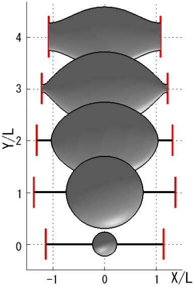
Figure 1: Embeddings of the spatial horizon geometry of various 6-d BHs and NUSs in 5-d Euclidean space (suitably projected onto the page). For BH solutions we include the exposed symmetry axis in the embedding. The red vertical lines are to be periodically identified, generating the compact dimension.

II Method

Both the non-uniform strings and black holes are static axisymmetric geometries that can be written in the form,

$$ds^{2}=-e^{2A}dt^{2}+e^{2B}\left(dr^{2}+dz^{2}\right)+e^{2C}r^{2}d\Omega^{2}_{d-3}$$ (1)

where $A,B,C$ are functions of $r,z$. We take these to vanish at large radial coordinate $r$, and hence the geometry is asymptotically $R^{1,d-2}\times S^{1}$. The circle coordinate $z$ has length $L$ asymptotically. We then employ a numerical method developed in Wiseman (2002, 2003a); Kudoh et al. (2003) which uses relaxation techniques to solve for $A,B,C$, whilst ensuring all the Einstein equations are satisfied. The reader is referred to Wiseman (2003a) for details of the procedure .

Following Townsend and Zamaklar (2001); Kol et al. (2004); Harmark and Obers (2004b, c), because the solutions are not asymptotically flat, they are characterised in terms of 2 asymptotic charges; the mass $M$ and a dimensionless tension $n$, which then give a first law, $dM=TdS+nM{dL}/{L}$ where $T,S$ are the black hole temperature and entropy.

In the following plots, we will fix the asymptotic circle length $L=1$ for all solutions shown, and then use the quantity $n$ to characterise the solutions. For small black holes $n\simeq 0$, and for uniform strings $n=1/(d-3)$. For convenience we normalise the thermodynamic quantities $T,S,M,n$ by their value for the critical uniform string, $T_{crit},S_{crit},M_{crit},n_{crit}$.

The most error prone part of the numerical calculation is extracting the asymptotic form of the metric in order to compute $M,n$. Particularly difficult is $n$ as it is constructed from the difference of two relatively large quantities Kudoh and Wiseman (2004). Here we compute both $n$ and $M$ using the first law and Smarr formula from $T$ and $S$, which are conveniently determined from the metric near the horizon.

III 6-D Results

We now discuss the behaviour of 6-d localised black holes, and the evidence that they join to the non-uniform branch. Firstly we consider the geometry of the horizon.

We may embed the spatial horizon geometry as a surface of revolution in 5-d Euclidean space. This is illustrated for several solutions in figure 1. The intrinsic geometry of the embedded surface is the same as that of the spatial sections of the 6-d horizons. Note that for the black holes we also include the exposed rotational symmetry axis in the embedding plots. The Euclidean coordinate along the surface of revolution, $X$, should be thought of as periodic with $-X_{max}<X<X_{max}$ being the fundamental domain plotted. Then $X_{max}$ gives a coordinate invariant measure of the ‘size’ of the geometry near the symmetry axis, and we plot this in figure 2.

For non-uniform solutions we may compute the maximum and minimum radii of the horizon $R_{max,min}$. Analogously, for the black holes we have $R_{eq}$, the equatorial radius of the horizon, and $L_{axis}$, the proper length along the exposed symmetry axis. These are plotted in figure 3.

From these graphs we see firstly that for increasing $n$ the equatorial radius of the black holes reaches a maximum and then starts to decrease, implying that there is indeed a maximum ‘size’ localised solution that can ‘fit’. Secondly, from the horizon geometry it is plausible that the non-uniform and black hole branches merge around $n/n_{crit}\simeq 0.55$, where the value of $R_{eq}$ appears to tend to $R_{max}$, and $X_{max}$ is consistent with an extrapolation that agrees between the branches for this value of $n/n_{crit}$.

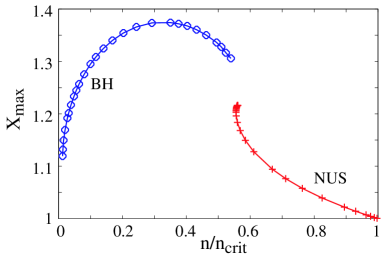
Figure 2: Plot of $X_{max}$ for 6-d NUSs and BHs, consistent with merger of the branches at $n/n_{crit}\simeq 0.55$.

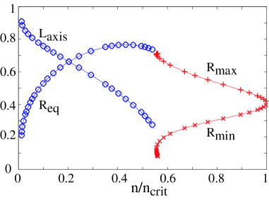
Figure 3: Plot of horizon geometric quantities for 6-d solutions. Branches are consistent with a topology changing merger where both $L_{axis}$ and $R_{min}$ go to zero, and $R_{eq}$ tends to $R_{max}$. All solutions have $L=1$.

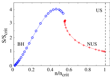
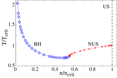
Figure 4: Entropy and temperature for 6-d solutions.

Now we consider thermodynamic quantities. In figures 4 and 5 we plot the entropy, temperature and mass of the solutions against $n$. Mirroring the behaviour of $R_{eq}$, we see the entropy and mass of the black holes reach a maximum and then decrease with increasing $n$. From this thermodynamic data we again clearly see evidence the branches merge.

Note that in our previous work Kudoh and Wiseman (2004) constructing the 6-d black holes the solutions were only found in the regime where $R_{eq}$ and the mass were increasing with $n$, and hence it was not clear that the two branches could unify.

For very small masses the localised black holes are entropically favoured, and for very large masses only the uniform strings exist. In figure 6 we plot the entropy against mass for the 3 branches. We see uniform strings become entropically favoured, for a given mass, at masses above that of the critical uniform string, but below that of the maximum mass localised black hole.

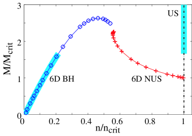
Figure 5: Mass against $n$ for 6-d solutions. The highlighting indicates which branch is entropically favoured for a given mass (see figure 6).

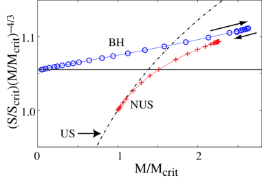
Figure 6: Plot of $SM^{-4/3}$ against mass for the 6-d solutions. 6-d Schwarzschild behaviour is $S\propto M^{4/3}$ so represents a horizontal line. We see the localised BHs are entropically favoured for a given mass, for $M<1.7M_{\mathrm{crit}}$. Above this mass the uniform strings are favoured. The NUSs are never dominant.

Thus we see that the branches appear consistent with merger at $n/n_{crit}\simeq 0.55$. Let us now assume that this occurs via a conical transition. We can then measure how far from the transition point the solutions are by estimating the geometric resolution of the cone. For the non-uniform strings this is given by the minimal radius of the horizon, $R_{min}$, which for the most non-uniform string found in Wiseman (2003a) was $R_{min}\simeq 0.08$ in our units where $L=1$. The resolution for the black hole is given by the proper distance of exposed symmetry axis, $L_{axis}$. For these 6-d solutions the smallest resolution found was $L_{axis}\simeq 0.27$. Therefore the most non-uniform strings found are still considerably closer to the assumed transition point than the most extreme localised black holes found here. For these non-uniform solutions the emergence of the cone geometry has been numerically demonstrated Kol and Wiseman (2003). Repeating this for our new black hole solutions does indeed show an increase in curvature on the axis consistent with an emerging cone, but as the solutions are ‘further’ from the transition point this increase in curvature is still not large enough to be clearly distinguished from the background curvature of the black hole geometry. Thus whilst our new 6-d black hole data is very suggestive the solution branches merge, it still cannot confirm that the detailed merger from the black hole side is via a conical transition. Indeed in Kol’s original picture Kol (2002b) we note that the cone may act only as an approximate local model for the merger, and the detailed behaviour very close to the point where the horizon pinches off may have a complicated behaviour that cannot necessarily be thought of as being smoothly resolvable.

IV 5-D Results

We now briefly discuss the 5-d black hole solutions. All quantities behave in an analogous manner to their counterparts for the 6-d solutions. Here we have simply plotted the mass against $n$ in figure 7. Note the mass increases past the critical uniform string mass with increasing $n$ (extending the previous numerical solutions in 5d Sorkin et al. (2004)), reaching a maximum and then decreases, again presumably to join the non-uniform branch.

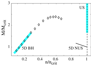
Figure 7: Mass against $n$ for new 5-d localised BHs. Highlighting indicates entropically favoured solution at a given mass.

Acknowledgements We would like to thank Ofer Aharony, Gary Horowitz, Barak Kol, Jo Marsano and Shiraz Minwalla for enjoyable and enlightening discussions. TW was supported by the David and Lucille Packard Foundation grant number 2000-13869A. HK is supported by the JSPS. Numerical computations were carried out at the YITP and NAO.

References

- Arkani-Hamed et al. (1998) N. Arkani-Hamed, S. Dimopoulos, and G. R. Dvali, Phys. Lett. B429, 263 (1998).
- Antoniadis et al. (1998) I. Antoniadis, N. Arkani-Hamed, S. Dimopoulos, and G. R. Dvali, Phys. Lett. B436, 257 (1998).
- Kol (2002a) B. Kol (2002a), eprint hep-ph/0207037.
- Itzhaki et al. (1998) N. Itzhaki, J. M. Maldacena, J. Sonnenschein, and S. Yankielowicz, Phys. Rev. D58, 046004 (1998).
- Susskind (1998) L. Susskind (1998), eprint hep-th/9805115.
- Martinec and Sahakian (1999) E. J. Martinec and V. Sahakian, Phys. Rev. D59, 124005 (1999).
- Li et al. (1999) M. Li, E. J. Martinec, and V. Sahakian, Phys. Rev. D59, 044035 (1999).
- Aharony et al. (2004) O. Aharony, J. Marsano, S. Minwalla, and T. Wiseman (2004), eprint hep-th/0406210.
- Harmark and Obers (2004a) T. Harmark and N. A. Obers (2004a), eprint hep-th/0407094.
- Kol (2002b) B. Kol (2002b), eprint [http://arXiv.org/abs]hep-th/0206220.
- Emparan and Reall (2002) R. Emparan and H. Reall, Phys. Rev. Lett. 88, 101101 (2002).
- Sorkin (2004) E. Sorkin, Phys. Rev. Lett. 93, 031601 (2004).
- Kol and Sorkin (2004) B. Kol and E. Sorkin (2004), eprint gr-qc/0407058.
- Harmark (2004) T. Harmark, Phys. Rev. D69, 104015 (2004).
- Gorbonos and Kol (2004) D. Gorbonos and B. Kol, JHEP 06, 053 (2004).
- Elvang et al. (2004) H. Elvang, T. Harmark, and N. A. Obers (2004), eprint hep-th/0407050.
- Gregory and Laflamme (1993) R. Gregory and R. Laflamme, Phys. Rev. Lett. 70, 2837 (1993).
- Choptuik et al. (2003) M. W. Choptuik et al., Phys. Rev. D68, 044001 (2003).
- Horowitz and Maeda (2001) G. Horowitz and K. Maeda, Phys. Rev. Lett. 87, 131301 (2001).
- Gubser (2002) S. Gubser, Class. Quant. Grav. 19, 4825 (2002).
- Harmark and Obers (2002) T. Harmark and N. Obers, JHEP 05, 032 (2002).
- Wiseman (2003a) T. Wiseman, Class. Quant. Grav. 20, 1137 (2003a).
- Wiseman (2003b) T. Wiseman, Class. Quant. Grav. 20, 1177 (2003b).
- Kol and Wiseman (2003) B. Kol and T. Wiseman, Class. Quant. Grav. 20, 3493 (2003).
- Kudoh and Wiseman (2004) H. Kudoh and T. Wiseman, Prog. Theor. Phys. 111, 475 (2004).
- Sorkin et al. (2004) E. Sorkin, B. Kol, and T. Piran, Phys. Rev. D69, 064032 (2004).
- Wiseman (2002) T. Wiseman, Phys. Rev. D65, 124007 (2002).
- Kudoh et al. (2003) H. Kudoh, T. Tanaka, and T. Nakamura, Phys. Rev. D68, 024035 (2003).
- Townsend and Zamaklar (2001) P. K. Townsend and M. Zamaklar, Class. Quant. Grav. 18, 5269 (2001).
- Kol et al. (2004) B. Kol, E. Sorkin, and T. Piran, Phys. Rev. D69, 064031 (2004).
- Harmark and Obers (2004b) T. Harmark and N. A. Obers, Nucl. Phys. B684, 183 (2004b).
- Harmark and Obers (2004c) T. Harmark and N. A. Obers, Class. Quant. Grav. 21, 1709 (2004c).
- Kleihaus and Kunz (1997) B. Kleihaus and J. Kunz, Phys. Rev. Lett. 79, 1595 (1997).