Non-Abelian Walls and Vortices in Supersymmetric Theories

Abstract

We review recent results on solitons in supersymmetric (SUSY) non-Abelian gauge theories, focusing on our papers: hep-th/0405194, hep-th/0405129, and hep-th/0404198. We construct the BPS multi-wall solutions in supersymmetric $U(N_{\rm C})$ gauge theories in five dimensions with $N_{\rm F}(>N_{\rm C})$ hypermultiplets in the fundamental representation. Exact solutions are obtained with full generic moduli for infinite gauge coupling. Total moduli space of the BPS non-Abelian walls is found to be the complex Grassmann manifold $SU(N_{\rm F})/[SU(N_{\rm C})\times SU(N_{\rm F}-{N}_{\rm C})\times U(1)]$. A 1/4 BPS equation is also studied which gives combinations of vortices, walls and monopoles. The full moduli space of the 1/4 BPS equation is found to be the space of all holomorphic maps from a complex plane to the wall moduli space. Exact solutions of the 1/4 BPS equation are also obtained for infinite gauge coupling.

Department of Physics, Tokyo Institute of Technology
Tokyo 152-8551, JAPAN

1 Introduction

Supersymmetric (SUSY) theories have been providing the most realistic models beyond the standard model [?]. In recent years, much attention has been devoted to models with extra dimension [?]–[?], where our four-dimensional world is realized on a topological defect in higher dimensional spacetime. It is desirable to obtain the topological defects as solitons in field theories. In constructing topological defects, supersymmetric theories are helpful, since partial preservation of SUSY automatically gives a solution of equations of motion [?]. These states are called BPS states. Moreover, the resulting theory tend to produce an ${\cal N}=1$ SUSY theory on the world volume, which can provide realistic unified models with the desirable properties. Supersymmetry also helps to obtain stability of the soliton. The simplest of such solitons is the domain wall [?]. It has been a difficult problem to localize massless gauge bosons on the wall in five dimensions, in spite of many interesting proposals, especially in lower dimensions [?]–[?]. Recently a model of the localized massless gauge bosons on the wall has been obtained for Abelian gauge theories using SUSY QED interacting with tensor multiplets [?,?]. Walls in non-Abelian gauge theories are likely to help obtaining non-Abelian gauge bosons localized on the world volume. We call these walls as non-Abelian walls. Non-Abelian wall solutions have rich structures and are also interesting in its own right.

Recently we have conducted a series of study to obtain various BPS solutions of a non-Abelian gauge theory with eight supercharges in spacetime dimensions of five or less [?]–[?]. More specifically, we have studied the $U(N_{\rm C})$ gauge theory with $N_{\rm F}(>N_{\rm C})$ flavors of hypermultiplets in the fundamental representation. To obtain discrete vacua, we consider non-degenerate masses for hypermultiplets, and the Fayet-Iliopoulos (FI) parameter is introduced [?]. We have obtained BPS multi-wall solutions as $1/2$ BPS solutions, and various combinations of walls, vortices and monopoles in the Higgs phase as $1/4$ BPS solutions. By taking the limit of infinite gauge coupling, we have obtained exact BPS multi-wall solutions with generic moduli parameters covering the complete moduli space of walls [?]. For a restricted class of moduli parameters called $U(1)$-factorizable moduli, we have obtained exact BPS multi-wall solutions for certain values of finite gauge coupling [?].

Since the BPS equations for the hypermultiplets $H^{i}$ involve the extra-dimensional component gauge field $W_{y}$ and the vector multiplet scalar as a function of the extra-dimensional coordinate $y$, it can be solved in terms of a $GL(N_{\rm C},{\bf C})$ gauge transformation matrix $S(y)$ as a function of the extra-dimensional coordinate $y$. Apart from the additional $y$ dependence due to the mass of each flavor, the hypermultiplet is thus given by a product [?] of $S(y)$ and $N_{\rm C}\times N_{\rm F}$ constant moduli matrices $H_{0}^{i}$. The BPS equation for the vector multiplet determines $S(y)$ once $H_{0}$ is given. Since the hypermultiplet depends only on the product $S^{-1}H_{0}$, this description has a redundancy of a global symmetry $GL(N_{\rm C},{\bf C})$ acting on $(S,H_{0}^{i})$, which we call the world-volume symmetry. Therefore the moduli space of $1/2$ BPS domain walls is given by a compact complex manifold, the Grassmann manifold [?] $G_{N_{\rm F},N_{\rm C}}\equiv{SU(N_{\rm F})\over SU(N_{\rm C})\times SU(N_{\rm F}-N_{\rm C})\times U(1)}$. One should note that this is the total moduli space of the multi-wall solutions including all the topological sectors. If we take a multi-wall configuration and let one of the wall going to infinity, we obtain a configuration with one less wall. Therefore configurations with smaller number of domain walls appear as boundaries of the moduli space. If we add all these different topological sectors, the total moduli space becomes the compact complex manifold $G_{N_{\rm F},N_{\rm C}}$.

The world-volume symmetry turned out to be very useful and will eventually be promoted to a local gauge symmetry when we consider effective theories on the world volume of walls.

If we consider a vortex perpendicular to a wall, it preserves a different combination of four supercharges compared to the wall [?]. We have found that the coexistence of the vortex and the wall can be realized as a $1/4$ BPS configuration [?]. We also found that this $1/4$ BPS equation admits also monopoles in the Higgs phase which were found recently [?]. We have obtained the exact solutions in the limit of infinite gauge coupling. We also identified the moduli space of the $1/4$ BPS solutions to be the space of all the holomorphic maps from the complex plane to the wall moduli space [?], the Grassmann manifold $G_{N_{\rm F},N_{\rm C}}$.

2 SUSY Vacua of $U(N_{\rm C})$ Gauge Theories

The minimum number of supercharges in five dimensions is eight. Building blocks of field theories with eight supercharges are vector multiplets and hypermultiplets. Since wall solutions require discrete vacua, we consider a gauge group with $U(1)$ factors besides semi-simple gauge group [?]. As the most natural non-Abelian gauge group, we choose $U_{\rm G}(N_{\rm C})$ gauge group. We denote the gauge group suffix and flavor group suffix in our fundamental theory by the uppercase letter G and F, respectively. Let us consider a five-dimensional SUSY model with minimal kinetic terms for vector and hypermultiplets. Physical bosonic fields of the vector multiplet are gauge field $W_{M}$, and a scalar $\Sigma$ in the adjoint representation of the $U_{\rm G}(N_{\rm C})$ gauge group. The fields in the vector multiplet such as $\Sigma$ are expressed by an $N_{\rm C}\times N_{\rm C}$ matrix. Physical bosonic field of the hypermultiplet is an $SU(2)_{R}$ doublet of complex scalars $H^{i},i=1,2$ which are assigned to the fundamental representation of $U_{\rm G}(N_{\rm C})$. We consider $N_{\rm F}$ flavors of hypermultiplets and combine them into an $N_{\rm C}\times N_{\rm F}$ matrix denoted as $H^{i}\equiv(H^{irA})$ with color $r=1,\cdots,N_{\rm C}$ and flavor $A=1,\cdots,N_{\rm F}$ indices. We denote space-time indices by $M,N,\cdots=0,1,2,3,4$ with the metric $\eta_{MN}={\rm diag}(+1,-1,-1,-1,-1)$. For simplicity, we take the same gauge coupling $g$ for $U(1)$ and $SU(N_{\rm C})$ factors. The eight supercharges allow only a few parameters in our model: gauge coupling constant $g$, the masses of $A$-th hypermultiplet $m_{A}$, and the FI parameter $c$ for the $U(1)_{\rm G}$ gauge group. Then the bosonic part of our Lagrangian reads (after eliminating the auxiliary fields)

$${\cal L}=-\frac{1}{2g^{2}}{\rm Tr}\left[F_{MN}F^{MN}\right]+\frac{1}{g^{2}}{\rm Tr}\left[{\cal D}_{M}\Sigma{\cal D}^{M}\Sigma\right]+{\rm Tr}\left[{\cal D}^{M}H^{i}({\cal D}_{M}H^{i})^{\dagger}\right]-V,$$ (1)

$$V \!\!\!= \!\!\!\frac{g^{2}}{4}{\rm Tr}\left[\left(H^{1}H^{1\dagger}-H^{2}H^{2\dagger}-c\mathbf{1}_{N_{\rm C}}\right)^{2}+4H^{2}H^{1\dagger}H^{1}H^{2\dagger}\right]$$ (2)

$$+{\rm Tr}\left[(\Sigma H^{i}-H^{i}M)(\Sigma H^{i}-H^{i}M)^{\dagger}\right],$$

where the mass matrix is defined as $(M)^{A}{}_{B}\equiv m_{A}\delta^{A}{}_{B}$, and the covariant derivatives as ${\cal D}_{M}\Sigma=\partial_{M}\Sigma+i[W_{M},\Sigma]$, ${\cal D}_{M}H^{i}=(\partial_{M}+iW_{M})H^{i}$, and field strength as $F_{MN}=\frac{1}{i}[{\cal D}_{M},{\cal D}_{N}]=\partial_{M}W_{N}-\partial_{N}W_{M}+i[W_{M},W_{N}]$. We assume non-degenerate mass parameters $m_{A}$ and choose the order of the mass parameters as $m_{A}>m_{A+1}$ for all $A$. Then the flavor symmetry reduces to $G_{\rm F}=U(1)_{\rm F}^{N_{\rm F}-1}$, where $U(1)_{\rm F}$ corresponding to the common phase is gauged by $U(1)_{\rm G}$ local gauge symmetry.

SUSY vacua are realized at vanishing vacuum energy, which requires both contributions from vector and hypermultiplets to vanish. Conditions of vanishing contribution from vector multiplet read

$$H^{1}H^{1\dagger}-H^{2}H^{2\dagger}=c\mathbf{1}_{N_{\rm C}},\quad H^{2}H^{1\dagger}=0.$$ (3)

Requiring the vanishing contribution to vacuum energy from hypermultiplets gives the SUSY condition for hypermultiplets as

$$\Sigma H^{i}-H^{i}M=0.$$ (4)

By local gauge transformations of $G$, we can always choose the vector multiplet scalar to be diagonal $\Sigma={\rm diag}(\Sigma_{1},\Sigma_{2},\cdots,\Sigma_{N_{C}})$. Then Eq. (4) becomes diagonal : $(\Sigma_{s}-m_{A})H^{isA}=0$, where $r$ and $A$ denote color and flavor indices. The condition $H^{2}H^{1\dagger}={0}$ in Eq.(3) is best satisfied by $H^{2}=0$, because of $c>0$. Eq.(3) demands that at least some of $H^{isA}$ have to be nonvanishing. Then Eq.(4) requires the corresponding vector multiplet scalar to be nonvanishing $\Sigma_{s}=m_{A}$. Since we assume non-degenerate masses for hypermultiplets, we find that only one flavor $A=A_{r}$ can be non-vanishing for each color component $r$ of hypermultiplet scalars $H^{irA}$ with

$$H^{1rA}=\sqrt{c}\,\delta^{A_{r}}{}_{A},\quad H^{2rA}=0.$$ (5)

Here we used global gauge transformations to eliminate possible phase factors. This is called the color-flavor locked vacuum. The vector multiplet scalar $\Sigma$ is determined as

$$\Sigma={\rm diag.}(m_{A_{1}},\,m_{A_{2}},\,\cdots,\,m_{A_{N_{\rm C}}}).$$ (6)

Now we see that $N_{\rm F}>N_{\rm C}$ is needed in order to obtain disconnected SUSY vacua appropriate for constructing walls. The vacua for $U(2)_{\rm G}$ gauge group are illustrated in Fig.1, using $\Sigma\equiv{\rm diag}.((\Sigma^{0}+\Sigma^{3})/2,(\Sigma^{0}-\Sigma^{3})/2)$.

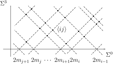
Figure 1: Diagrammatic representation of vacua for $N_{\rm C}=2$ case. Dashed lines are defined by $\Sigma^{0}+\Sigma^{3}=2m_{A}$ and $\Sigma^{0}-\Sigma^{3}=2m_{A}$. Vacua are given as intersection points of these lines except for $\Sigma^{3}=0$, because of $H^{2}H^{1\dagger}=0$ in Eq. (3).

We denote a SUSY vacuum specified by a set of non-vanishing hypermultiplet scalars with the flavor $\{A_{r}\}$ for each color component $r$ as

$$\langle A_{1}\,A_{2}\,\cdots\,A_{N_{\rm C}}\rangle.$$ (7)

Since global gauge transformations can exchange flavors $A_{r}$ and $A_{s}$ for the color component $r$ and $s$, respectively, the ordering of the flavors $A_{1},\cdots,A_{N_{\rm C}}$ does not matter in considering only vacua: $\langle 123\rangle=\langle 213\rangle$. Thus a number of SUSY vacua is given by [?]

$${}_{N_{\rm F}}C_{N_{\rm C}}={N_{\rm F}!\over N_{\rm C}!(N_{\rm F}-N_{\rm C})!}$$ (8)

and we usually take $A_{1}<A_{2}<\cdots<A_{N_{\rm C}}$.

3 BPS Equations for Walls

Walls interpolate between two vacua at $y=\infty$ and $y=-\infty$. These boundary conditions at $y=\pm\infty$ define topological sectors. When we consider walls, it is often convenient to fix a gauge in presenting solutions. The gauge transformations allow us to eliminate all the vector multiplet scalars $\Sigma^{I\not\in{\cal H}}$ for generators outside of the Cartan subalgebra ${\cal H}$, and all the gauge fields $W_{y}^{I\in{\cal H}}$ in the Cartan subalgebra ${\cal H}$. In this gauge, gauge fields $W_{y}^{I\not\in{\cal H}}$ can no longer be eliminated, since gauge is completely fixed. We usually use this gauge

$$\Sigma^{I\not\in{\cal H}}=0,\qquad W_{y}^{I\in{\cal H}}=0.$$ (9)

If we wish, we can choose another gauge where the extra dimension component $W_{y}^{I}$ of the gauge field vanishes for all the generators. Then all components of vector multiplet scalars $\Sigma^{I}$ including those out of Cartan subalgebra become nontrivial. In that gauge, our BPS multi-wall solutions are expressed by nontrivial vector multiplet scalars $\Sigma^{I}$ for all the generators, instead of gauge fields $W_{y}^{I}$. Our explicit solutions show that the gauge field content is generically nontrivial, since we cannot eliminate all of $W_{y}^{I}$ and $\Sigma^{I}$ : either $W_{y}^{I}\not=0$ or $\Sigma^{I}\not=0$ in any gauge.

To obtain domain walls, we assume that all fields depend only on the coordinate of one extra dimension $x^{4}$ which we denote as $y$. We also assume the Poincaré invariance on the four-dimensional world volume of the wall, implying

$$F_{MN}(W)=0,\ \ W_{\mu}=0,$$ (10)

where we take $x^{\mu}=(x^{0},x^{1},x^{2},x^{3})$ as four-dimensional world-volume coordinates. Note that $W_{y}$ need not vanish. The Bogomol’nyi completion of the energy density of our system can be performed as

$${\cal E} = \frac{1}{g^{2}}{\rm Tr}\left[({\cal D}_{y}\Sigma)^{2}\right]+{\rm Tr}\left[{\cal D}^{M}H^{i}({\cal D}_{M}H^{i})^{\dagger}\right]+{\rm Tr}\left[(\Sigma H^{i}-H^{i}M)(\Sigma H^{i}-H^{i}M)^{\dagger}\right]$$ (11)

$$+\frac{g^{2}}{4}{\rm Tr}\Big{[}\left(H^{1}H^{1\dagger}-H^{2}H^{2\dagger}-c\mathbf{1}_{N_{\rm C}}\right)^{2}+4H^{2}H^{1\dagger}H^{1}H^{2\dagger}\Big{]}$$

$$= \frac{1}{g^{2}}{\rm Tr}\left({\cal D}_{y}\Sigma-{g^{2}\over 2}\left(c{\bf 1}_{N_{\rm C}}-H^{1}H^{1}{}^{\dagger}+H^{2}H^{2}{}^{\dagger}\right)\right)^{2}+{g^{2}}{\rm Tr}\Big{[}H^{2}H^{1\dagger}H^{1}H^{2\dagger}\Big{]}$$

$${}+{\rm Tr}\left[({\cal D}_{y}H^{1}+\Sigma H^{1}-H^{1}M)({\cal D}_{y}H^{1}+\Sigma H^{1}-H^{1}M)^{\dagger}\right]$$

$${}+{\rm Tr}\left[({\cal D}_{y}H^{2}-\Sigma H^{2}+H^{2}M)({\cal D}_{y}H^{2}-\Sigma H^{2}+H^{2}M)^{\dagger}\right]$$

$${}+c\partial_{y}{\rm Tr}\Sigma-\partial_{y}\left\{{\rm Tr}\left[\left(\Sigma H^{1}-H^{1}M\right)H^{1}{}^{\dagger}+\left(-\Sigma H^{2}+H^{2}M\right)H^{2}{}^{\dagger}\right]\right\}.$$

Therefore we obtain a lower bound for the energy of the configuration. By saturating the complete squares, we obtain the BPS equation

$${\cal D}_{y}\Sigma={g^{2}\over 2}\left(c{\bf 1}_{N_{\rm C}}-H^{1}H^{1}{}^{\dagger}+H^{2}H^{2}{}^{\dagger}\right),\quad 0=g^{2}H^{1}H^{2}{}^{\dagger},$$ (12)

$${\cal D}_{y}H^{1}=-\Sigma H^{1}+H^{1}M,\qquad{\cal D}_{y}H^{2}=\Sigma H^{2}-H^{2}M.$$ (13)

The BPS saturated configuration satisfying the BPS Eqs. (12)-(13) gives the minimum energy (per unit volume), namely the tension of the BPS wall as

$$T_{\rm w} \!\!=\!\! \!\!\int^{+\infty}_{-\infty}dy{\cal E}=c\left[{\rm Tr}\Sigma\right]^{+\infty}_{-\infty}\!\!=\!c\left(\sum_{k=1}^{N_{\rm C}}m_{A_{k}}-\sum_{k=1}^{N_{\rm C}}m_{B_{k}}\right),$$ (14)

if we choose a boundary condition approaching to a SUSY vacuum labeled by $\langle A_{1}A_{2}\cdots A_{N_{\rm C}}\rangle$ at $y=+\infty$, and to a vacuum $\langle B_{1}B_{2}\cdots B_{N_{\rm C}}\rangle$ at $y=-\infty$. Since the vacuum condition $\Sigma H^{i}-H^{i}M=0$ is satisfied at $y=\pm\infty$, the second term of the last line of Eq. (11) does not contribute.

The BPS Eqs. (12), (13) are equivalent to the preservation condition of the half of the supercharges [?].

4 BPS Wall Solutions

The vector multiplet scalar $\Sigma$ can be obtained as the sixth component of the six-dimensional vector multiplet through the dimensional reduction. It is thus natural to combine the fifth component gauge field $W_{y}$ with the vector multiplet scalar to form a complexified gauge field $\Sigma+iW_{y}$. Since it is merely a function of $y$, we can eliminate it through an $N_{\rm C}\times N_{\rm C}$ invertible complex matrix function $S(y)$ representing a complexified gauge transformation defined as

$$\Sigma+iW_{y}\equiv S^{-1}\partial_{y}S.$$ (15)

Note that this differential equation determines the function $S(y)$ with $N_{\rm C}^{2}$ arbitrary complex integration constants, from which the world-volume symmetry emerges as we see later. Let us change variables from $H^{1},\,H^{2}$ to $N_{\rm C}\times N_{\rm F}$ matrix functions $f^{1},\,f^{2}$ by using $S$

$$H^{1}\equiv S^{-1}f^{1},\quad H^{2}\equiv S^{\dagger}f^{2}.$$ (16)

Substituting (15), (16) to the BPS Eq. (13) for $H^{i}$, we obtain

$$\partial_{y}f^{1}=f^{1}M,\quad\partial_{y}f^{2}=-f^{2}M$$ (17)

which can be easily solved as

$$f^{1}=H_{0}^{1}\,e^{My},\quad f^{2}=H^{2}_{0}e^{-My}$$ (18)

with the $N_{\rm C}\times N_{\rm F}$ constant complex matrices $H_{0}^{1},\,H^{2}_{0}$ as integration constants, which we call moduli matrices. Therefore $H^{i}$ can be solved completely in terms of $S$ as

$$H^{1}=S^{-1}H_{0}^{1}e^{My},\quad H^{2}=S^{\dagger}H_{0}^{2}e^{-My}.$$ (19)

The definitions (15), (16) show that a set $(S,H_{0}^{1},H_{0}^{2})$ and another set $(S^{\prime},H_{0}^{1}{}^{\prime},H_{0}^{2}{}^{\prime})$ give the same original fields $\Sigma,\,W_{y},H^{i}$, provided they are related by

$$S^{\prime}=VS,\quad H_{0}^{1}{}^{\prime}=VH_{0}^{1},\quad H_{0}^{2}{}^{\prime}=(V^{\dagger})^{-1}H_{0}^{2},$$ (20)

where $V\in GL(N_{\rm C},{\bf C})$. This transformation $V$ defines an equivalence class among sets of the matrix function and moduli matrices $(S,H_{0}^{1},H_{0}^{2})$ which represents physically equivalent results. This symmetry comes from the $N_{\rm C}^{2}$ integration constants in solving (15), and represents the redundancy of describing the wall solution in terms of $(S,H_{0}^{1},H_{0}^{2})$. We call this ‘world-volume symmetry’, since this symmetry will be promoted to a local gauge symmetry in the world volume of walls when we consider the effective action on the walls.

Since $H^{2}$ vanishes in any SUSY vacuum as given in Eq. (5) as a result of non-degenerate masses, which we consider here. Thus the moduli matrix for domain walls $H^{2}_{0}$ corresponding to the field $H^{2}$ also vanishes as shown in Appendix C of Ref. [?]. Consequently the field $H^{2}$ for domain wall solutions vanishes identically in the extra dimension. Therefore we take

$$H^{2}_{0}=0,\qquad(H^{2}=0),\qquad H_{0}\equiv H^{1}_{0}.$$ (21)

The remaining BPS equations for the vector multiplets can be written in terms of the matrix $S$ and the moduli matrix $H_{0}$. Since the matrix function $S$ originates from the vector multiplet scalars $\Sigma$ and the fifth component of the gauge fields $W_{y}$ as in Eq. (15), the gauge transformations $U(y)$ on the original fields $\Sigma,\,W_{y},\,H^{1},\,H^{2}$

$$H^{1} \rightarrow H^{1}{}^{\prime}=UH^{1},\qquad H^{2}\rightarrow H^{2}{}^{\prime}=UH^{2},$$

$$\Sigma+iW_{y} \rightarrow \Sigma^{\prime}+iW_{y}^{\prime}=U\left(\Sigma+iW_{y}\right)U^{\dagger}+U\partial_{y}U^{\dagger},\qquad$$ (22)

can be obtained by multiplying a unitary matrix $U^{\dagger}(y)$ from the right of $S$:

$$S\,\rightarrow\,S^{\prime}=SU^{\dagger},\quad U^{\dagger}U=1,$$ (23)

without causing any transformations on the moduli matrices $H_{0}$. Thus we define

$$\Omega\equiv SS^{\dagger},$$ (24)

which is invariant under the gauge transformations (23) of the fundamental theory. Note that this $\Omega$ is not invariant under the world-volume symmetry transformations (20):

$$\Omega\ \rightarrow\ \Omega^{\prime}=V\Omega V^{\dagger}.$$ (25)

Together with the gauge invariant moduli matrix $H_{0}$, the BPS equations (12) for vector multiplets can be rewritten in the following gauge invariant form

$$\partial_{y}^{2}\Omega-\partial_{y}\Omega\Omega^{-1}\partial_{y}\Omega=g^{2}\left(c\,\Omega-H_{0}\,e^{2My}H_{0}{}^{\dagger}\right).$$ (26)

Once a solution of $\Omega$ for Eq. (26) with a given moduli matrix $H_{0}$ is obtained, the matrix $S$ in Eq. (24) can be determined with a suitable gauge choice, and then all the quantities, $\Sigma,\,W_{y},\,H^{1}$ and $H^{2}$ are obtained by Eqs. (15) and (19). Since two boundary conditions are imposed at $y=\infty$ and at $y=-\infty$ to the second order differential equation (26), the number of necessary boundary conditions precisely matches to obtain the unique solution. Therefore there should be no more moduli parameters in addition to the moduli matrix $H_{0}$. In the limit of infinite gauge coupling, we find explicitly that there is no additional moduli. We have also analyzed in detail the almost analogous nonlinear differential equation in the case of the Abelian gauge theory at finite gauge coupling and find no additional moduli [?]. For the case of non-Abelian gauge theories at finite gauge coupling, there is no reason to believe a behavior different from the Abelian counterpart.

5 Moduli Space for Non-Abelian Walls

All possible solutions of parallel domain walls in the $U(N_{\rm C})$ SUSY gauge theory with $N_{\rm F}$ hypermultiplets can be constructed once the moduli matrix $H_{0}$ is given. The moduli matrix $H_{0}$ has a redundancy expressed as the world-volume symmetry (20) : $H_{0}\sim VH_{0}$ with $V\in GL(N_{\rm C},{\bf C})$. We thus find that the moduli space denoted by ${\cal M}_{N_{\rm F},N_{\rm C}}$ is homeomorphic to the complex Grassmann manifold ($\tilde{N}_{\rm C}\equiv N_{\rm F}-N_{\rm C}$) :

$${\cal M}_{N_{\rm F},N_{\rm C}}\simeq\{H_{0}|H_{0}\sim VH_{0},V\in GL(N_{\rm C},{\bf C})\}\simeq G_{N_{\rm F},N_{\rm C}}\simeq{SU(N_{\rm F})\over SU(N_{\rm C})\times SU(\tilde{N}_{\rm C})\times U(1)}\,.$$ (27)

This is a compact (closed) set. On the other hand, for instance, scattering of two Abelian walls is described by a nonlinear sigma model on a non-compact moduli space [?,?]. This fact of the compact moduli space consisting of non-compact moduli parameters can be consistently understood, if we note that the moduli space ${\cal M}_{N_{\rm F},N_{\rm C}}$ includes all BPS topological sectors determined by the different boundary conditions. It is decomposed into

$${\cal M}_{N_{\rm F},N_{\rm C}}=\sum_{\rm BPS}{\cal M}^{\langle B_{1}B_{2}\cdots B_{N_{\rm C}}\rangle\leftarrow\langle A_{1}A_{2}\cdots A_{N_{\rm C}}\rangle}_{N_{\rm F},N_{\rm C}},\;$$ (28)

where the sum is taken over the BPS sectors. Note that it also includes the vacuum states with no walls $\langle A_{1}A_{2}\cdots A_{N_{\rm C}}\rangle\leftarrow\langle A_{1}A_{2}\cdots A_{N_{\rm C}}\rangle$ which correspond to $N_{\rm F}!/N_{\rm C}!\tilde{N}_{\rm C}!$ points on the moduli space. Although each sector (except for vacuum states) is in general not a closed set, the total space is compact. We call ${\cal M}_{N_{\rm F},N_{\rm C}}$ as the “total moduli space”. It is useful to rewrite this as a sum over the number of walls:

$${\cal M}_{N_{\rm F},N_{\rm C}}=\sum_{k=0}^{N_{\rm C}\tilde{N}_{\rm C}}{\cal M}_{N_{\rm F},N_{\rm C}}^{k}={\cal M}_{N_{\rm F},N_{\rm C}}^{0}\oplus{\cal M}_{N_{\rm F},N_{\rm C}}^{1}\oplus\cdots\oplus{\cal M}_{N_{\rm F},N_{\rm C}}^{N_{\rm C}\tilde{N}_{\rm C}}\,,$$ (29)

with ${\cal M}_{N_{\rm F},N_{\rm C}}^{k}$ the sum of the topological sectors with $k$-walls. Since the maximal number of walls is $N_{\rm C}\tilde{N}_{\rm C}$, ${\cal M}_{N_{\rm F},N_{\rm C}}^{N_{\rm C}\tilde{N}_{\rm C}}$ is identical to the maximal topological sector.

This decomposition can be understood as follows. Consider a $k$-wall solution and imagine a situation such that one of the outer-most walls goes to spatial infinity. We will obtain a ($k-1$)-wall configuration in this limit. This implies that the $k$-wall sector in the moduli space is an open set compactified by the moduli space of ($k-1$)-wall sectors on its boundary. Continuing this procedure we will obtain a single wall configuration. Pulling it out to infinity we obtain a vacuum state in the end. A vacuum corresponds to a point as a boundary of a single wall sector in the moduli space. The $k=0$ sector comprises a set of $N_{\rm F}!/N_{\rm C}!\tilde{N}_{\rm C}!$ points and does not have any boundary. Summing up all sectors, we thus obtain the total moduli space ${\cal M}_{N_{\rm F},N_{\rm C}}$ as a compact manifold. Note again that we include zero-wall sector, vacua without any walls.

The authors in Ref. [?] constructed a solution of the 1/4 BPS equation in a $D=4$, ${\cal N}=2$ SUSY theory with $N_{\rm C}=1,N_{\rm F}=2$. It is a composite soliton made of a wall and vortices (strings) ending on it. Topological stability of this composite soliton can be understood by interpreting vortices as sigma model lumps in the effective theory on the wall if and only if we consider the total moduli space (27) as the target space instead of the one-wall topological sector ${\cal M}_{2,1}^{k=1}\simeq{\bf R}\times S^{1}$. This is because the second homotopy group $\pi_{2}$ ensuring the topological stability of lumps is ${\bf Z}$ for ${\bf C}P^{1}$ but is trivial for ${\bf R}\times S^{1}$. The total moduli space (27) for general $N_{\rm F}$ and/or $N_{\rm C}$ provides the topological stability of more complicated composite solitons which will be discussed in Sec.8 [?].

6 Infinite Gauge Coupling and Nonlinear Sigma Models

The BPS equation (26) for the gauge invariant $\Omega$ reduces to an algebraic equation in the strong gauge coupling limit, given by

$$\Omega_{g\to\infty}=(SS^{\dagger})_{g\to\infty}=c^{-1}H_{0}e^{2My}H_{0}^{\dagger}.$$ (30)

Therefore in the infinite gauge coupling we do not have to solve the second order differential equation for $\Omega$ and can explicitly construct wall solutions once the the moduli matrix $H_{0}$ is given. Qualitative behavior of walls for finite gauge couplings is not so different from that in infinite gauge couplings. This is because the right hand side of Eq. (26) tend to zero at both spatial infinities even for finite $g$. Hence wall solutions for finite $g$ asymptotically coincides with those for infinite $g$, and they differ only at finite region. In fact in [?] we have constructed exact wall solutions for finite gauge couplings and found that their qualitative behavior is the same as the infinite gauge coupling cases found in the literature [?,?].

SUSY gauge theories reduce to nonlinear sigma models in general in the strong gauge coupling limit $g_{0},\ g\to\infty$. Since the BPS equations are drastically simplified to become solvable in some cases, we often consider this limit. In fact the BPS domain walls in theories with eight supercharges were first obtained in hyper-Kähler (HK) nonlinear sigma models [?]. They have been the only known examples for models with eight supercharges [?,?] until exact wall solutions at finite gauge coupling were found recently [?,?,?]. If hypermultiplets have masses, the corresponding nonlinear sigma models have potentials, which can be written as the square of the tri-holomorphic Killing vector on the target manifold [?]. These models are called massive HK nonlinear sigma models. By this potential most vacua are lifted leaving some discrete degenerate points as vacua, which are characterized by fixed points of the Killing vector. In these models interesting composite $1/4$ BPS solitons like intersecting walls [?], intersecting lumps [?] and composite of wall-lumps [?,?] were constructed.

In our case of $U(N_{\rm C})$ gauge theory with $N_{\rm F})$ flavors of fundamental representation, the target space of the HK nonlinear sigma model is the cotangent bundle over the complex Grassmann manifold [?,?] ($\tilde{N}_{\rm C}\equiv N_{\rm F}-N_{\rm C}$)

$${\cal M}^{M=0}_{\rm vac}\simeq T^{*}G_{N_{\rm F},N_{\rm C}}\simeq T^{*}\left[SU(N_{\rm F})\over SU(N_{\rm C})\times SU(\tilde{N}_{\rm C})\times U(1)\right]\,.$$ (31)

From the target manifold (31) one can easily see that there exists a duality between theories with the same flavor and two different gauge groups in the case of the infinite gauge coupling [?,?]: $U(N_{\rm C})\leftrightarrow U(\tilde{N}_{\rm C})$. This duality holds for the Lagrangian of the nonlinear sigma models, and leads to the duality between the BPS equations of these two theories. This duality holds also for the moduli space of domain wall configurations.

We can obtain the effective action on the world volume of walls, by promoting the moduli parameters to fields on the world volume [?]. In the case of infinite gauge coupling, the Kähler potential of the effective Lagrangian is given by [?]

$${\cal L}_{\rm walls}^{g\to\infty}=c\int d^{4}\theta\int dy\ \log\det\Omega_{g\to\infty}=c\int d^{4}\theta\int dy\ \log\det(H_{0}e^{2My}H_{0}{}^{\dagger})\;.$$ (32)

7 Penetrable and Impenetrable Walls

Let us first take the $U(1)$ gauge theory to clarify the physical meaning of the moduli matrix $H_{0}$, which can be parametrized generically by complex moduli parameters $e^{r_{A}}$ as

$$H_{0}=\sqrt{c}(e^{r_{1}},e^{r_{2}},\cdots,e^{r_{N_{F}}}).$$ (33)

Because of the world-volume symmetry (20), only the relative magnitude has physical meaning: we can fix $e^{r_{1}}=1$, for instance. Then we obtain the hypermultiplet scalars as

$$H=S^{-1}H_{0}e^{My}=S^{-1}\sqrt{c}(e^{r_{1}+m_{1}y},\cdots,e^{r_{N_{F}}+m_{N_{F}}y}).$$ (34)

Figure 2: Region of rapid change of hypermultiplets indicates the positions of walls.

The relative magnitude of different flavors varies as $y$ varies because of the nondegenerate masses of the hypermultiplets, indicating that the solution approaches various vacua successively at various $y$. When $A$-th and $A+1$-th flavors becomes comparable each other, the transition between two adjacent vacua occurs. This is the location Re$Y_{A}$ of the wall separating the $A$- and $A+1$-th vacua, which is determined in terms of the relative magnitude of different flavors of the moduli matrix elements as $Y_{A}\equiv-{r_{A}-r_{A+1}\over m_{A}-m_{A+1}}$. The imaginary part Im$Y_{A}$ of the moduli gives the relative phase between adjacent vacua. The overall normalization is taken care of by the function $S^{-1}(y)$. Consequently the hypermultiplet scalars exhibit the multi-wall behavior as illustrated in Fig. 2 for the case of $N_{\rm F}=4$ ($N_{\rm C}=1$).

For multi-walls, we can define the relative distance of the walls as a difference of two wall positions $R_{A}=Y_{A}-Y_{A+1}$. If we let $R_{A}\rightarrow\infty$, we obtain two well-separated walls. For negative values of the relative distance, two walls merge together into a sharp single peak. Even in the limit of $R_{A}\rightarrow-\infty$, we still find a single peak with somewhat smaller width, namely a compressed wall. We call such a pair of walls as impenetrable. In the case of Abelian gauge theories, only the impenetrable walls can occur [?,?].

The $N_{\rm C}=2,\ N_{\rm F}=4$ case is the simplest example exhibiting a new feature of non-Abelian walls: there exists a pair of walls whose positions can commute with each other. Let us consider the topological sector labeled by $\langle 13\rangle\leftarrow\langle 24\rangle$. A moduli matrix for this sector $H_{0\langle 13\leftarrow 24\rangle}$ is given by two complex moduli parameters $r_{2},r_{3}$ after fixing the world-volume symmetry

$$H_{0\langle 13\leftarrow 24\rangle}=\sqrt{c}\left(\begin{array}[]{cccc}1&e^{r_{3}}&0&0\\ 0&0&1&e^{r_{2}}\end{array}\right).$$ (37)

We notice that this moduli matrix factorizes into $U(1)$ cases, which is called $U(1)$-factorizable, and that a solution obtained with this moduli matrix is given by

$$\Sigma^{0}+\Sigma^{3} = {m_{1}e^{2m_{1}y}+m_{2}e^{2m_{2}y+2{\rm Re}(r_{3})}\over e^{2m_{1}y}+e^{2m_{2}y+2{\rm Re}(r_{3})}},$$

$$\Sigma^{0}-\Sigma^{3} = {m_{3}e^{2m_{3}y}+m_{4}e^{2m_{4}y+2{\rm Re}(r_{2})}\over e^{2m_{3}y}+e^{2m_{4}y+2{\rm Re}(r_{2})}}$$ (38)

and $\Sigma^{1}=\Sigma^{2}=W_{y}=0$, and

Figure 3: Penetrable walls of $\langle 13\leftarrow 24\rangle$ in $N_{\rm C}=2$, $N_{\rm F}=4$ case. $M={\rm diag.}({3\over 2},{1\over 2},-{1\over 2},-{3\over 2})$. a) $r_{3}=5,\,r_{2}=-5$: the intermediate region shows $\langle 23\rangle$ vacuum. b) $r_{3}=-5,\,r_{2}=5$, $c=1$: the intermediate region shows $\langle 14\rangle$ vacuum.

$$H^{1}=\sqrt{c}\left(\begin{array}[]{cccc}{e^{m_{1}y}\over\sqrt{e^{2m_{1}y}+e^{2m_{2}y+2{\rm Re}(r_{3})}}}&{e^{m_{2}y+r_{3}}\over\sqrt{e^{2m_{1}y}+e^{2m_{2}y+2{\rm Re}(r_{3})}}}&0&0\\ 0&0&{e^{m_{3}y}\over\sqrt{e^{2m_{3}y}+e^{2m_{4}y+2{\rm Re}(r_{2})}}}&{e^{m_{4}y+r_{2}}\over\sqrt{e^{2m_{3}y}+e^{2m_{4}y+2{\rm Re}(r_{2})}}}\end{array}\right).$$ (41)

Profiles of $\Sigma^{0}\pm\Sigma^{3}$ and $H^{1}$ are illustrated in Fig. 3. This solution describes a configuration of double wall. In this case, position of the walls are given by $y_{3}={{\rm Re}(r_{3})\over m_{1}-m_{2}}$, and $y_{2}={{\rm Re}(r_{2})\over m_{3}-m_{4}}$. In a region $y_{2}>y_{3}$, the configuration interpolates between vacua $\langle 13\rangle$ and $\langle 24\rangle$ through the vicinity of the vacuum $\langle 14\rangle$. The wall at $y_{2}$ ($y_{3}$) interpolates between vacua $\langle 13\rangle$ and $\langle 14\rangle$ ($\langle 24\rangle$ and $\langle 14\rangle$). On the other hand, in a region $y_{3}>y_{2}$ the wall at $y_{3}$ ($y_{2}$) interpolates as $\langle 13\rangle\leftarrow\langle 23\rangle$ ($\langle 23\rangle\leftarrow\langle 24\rangle$). Note that while intermediate vacua are different from one region $(y_{3}>y_{2})$ to the other $(y_{3}<y_{2})$, the two parameters $y_{2},y_{3}$ retain the physical meaning as positions of the walls. The wall represented by the position $y_{2}$ changes flavors of non-vanishing hypermultiplet scalar from 4 to 3 and changes the value of $\Sigma^{0}-\Sigma^{3}$, while the wall at $y_{3}$ changes flavors from 2 to 1 and changes $\Sigma^{0}+\Sigma^{3}$. Thus, it is quite natural to identify the wall represented by the same parameter, although interpolated vacua are different. With this identification, we find that these two walls maintain their identity after passing through each other. Therefore we call the pair of walls as penetrable walls [?].

We also found that these properties of non-Abelian walls can be conveniently summarized by means of walls operators acting on the moduli space [?].

8 Vortices with Walls

If we make the moduli matrix $H_{0}$ to depend on the world volume coordinates, the wall location should depend on the position in the world volume. Then the walls will in general be curved and a magnetic field is generated. If we have a zero in $H_{0}$, it will give us a spike-like behavior of the wall, which becomes a vortex ending at the wall [?]. Similarly, if we allow an exponential dependence on the world volume coordinates for the moduli matrix elements, the wall can tilt. A vortex alone preserves a different combination of $1/2$ of supercharges compared to the wall perpendicular to the vortex. In fact we have found that the addition of vortex perpendicular to the walls can preserve $1/2$ of the surviving SUSY on the world volume of the wall. Consequently the combined configuration preserves $1/4$ of the original SUSY.

We assume the vortices depend on $x^{1},x^{2}$ and walls on $x^{3}$ (the combined configuration depends on $x^{m}\equiv x^{1},x^{2},x^{3}$ : co-dimension three) and assume Poincaré invariance in $x^{0},x^{4}$. Then we obtain $W_{0}=W_{4}=0$. Using the arguments for the walls, we take $H^{2}=0$. Requiring the SUSY transformation of fermions to vanish along the above $1/4$ SUSY directions, a set of 1/4 BPS equations is obtained. The wall BPS equation has an additional contribution of vortex magnetic field $F_{12}$

$${\cal D}_{3}\Sigma = {g^{2}\over 2}\left(c{\bf 1}_{N_{\rm C}}-H^{1}H^{1}{}^{\dagger}\right)+F_{12},\quad{\cal D}_{3}H^{1}=-\Sigma H^{1}+HM,$$ (42)

which is supplemented by the BPS equations for vortices

$$0 = {\cal D}_{1}H^{1}+i{\cal D}_{2}H^{1},\quad 0=F_{23}-{\cal D}_{1}\Sigma,\quad 0=F_{31}-{\cal D}_{2}\Sigma.$$ (43)

We have found that this set of $1/4$ BPS equations allows the recently found monopole in the Higgs phase [?].

We obtain the BPS bound of the energy density $\cal E$ as ${\cal E}\geq t_{\rm w}+t_{\rm v}+t_{\rm m}+\partial_{m}J_{m}$ with $t_{\rm w},\,t_{\rm v}$ and $t_{\rm m}$ the energy densities for walls, vortices and monopoles, and the correction term $J_{m}$, which does not contribute for individual walls and vortices

$$t_{\rm w} = c\partial_{3}{\rm Tr}\Sigma,\quad t_{\rm v}=-c{\rm Tr}\!F_{12},\quad t_{\rm m}=\frac{2}{g^{2}}\partial_{m}{\rm Tr}(\frac{1}{2}\epsilon^{mnl}\!F_{nl}\Sigma),$$ (44)

$$J_{1} = {\rm Re}\left(-i{\rm Tr}(H_{i}^{\dagger}{\cal D}_{2}H^{i})\right),\,J_{2}={\rm Re}\left(i{\rm Tr}(H_{i}^{\dagger}{\cal D}_{1}H^{i})\right),$$

$$J_{3} = -{\rm Tr}(H^{\dagger}_{i}(\Sigma-M)H^{i}).$$ (45)

Let us note that the magnetic flux from our monopole is measured in terms of the dual field strength multiplied (projected) by the Higgs field $\frac{1}{2}\epsilon^{mnl}\!F_{nl}\Sigma$, as is usual to obtain the $U(1)$ field strength for the monopole in the Higgs phase [?].

It is crucial to observe that Eq. (43) guarantees the integrability condition $[{\cal D}_{1}+i{\cal D}_{2},\,{\cal D}_{3}+\Sigma]=[\partial_{1}+i\partial_{2},\,\partial_{3}]=0$. Therefore we can introduce an $N_{\rm C}\times N_{\rm C}$ invertible complex matrix function $S(x^{m})\in GL(N_{\rm C},\mathbf{C})$ defined by

$$\Sigma+iW_{3} \equiv S^{-1}\partial_{3}S,\quad\left(({\cal D}_{3}+\Sigma)S^{-1}=0\right),$$ (46)

$$W_{1}+iW_{2} \equiv -2iS^{-1}\bar{\partial}S,\,\left(({\cal D}_{1}+i{\cal D}_{2})S^{-1}=0\right),\quad$$ (47)

where $z\equiv x^{1}+ix^{2}$, and $\bar{\partial}\equiv\partial/\partial z^{*}$. With (46) and (47), other Eqs. (43) are automatically satisfied, or are easily solved without any assumptions by

$$H^{1}=S^{-1}(z,z^{*},x^{3})H_{0}(z)e^{Mx^{3}}.$$ (48)

Here $H_{0}(z)$ is an arbitrary $N_{\rm C}\times N_{\rm F}$ matrix whose elements are arbitrary holomorphic functions of $z$. We call it “moduli matrix”.

Defining an $N_{\rm C}\times N_{\rm C}$ Hermitian matrix $\Omega\equiv SS^{\dagger}$, invariant under the $U(N_{\rm C})$ gauge transformations, we obtain the remaining BPS equation in Eq. (43)

$$4\partial\bar{\partial}\Omega-4(\partial\Omega)\Omega^{-1}(\bar{\partial}\Omega)+\partial_{3}^{2}\Omega-(\partial_{3}\Omega)\Omega^{-1}(\partial_{3}\Omega)=g^{2}\left(c\,\Omega-H_{0}\,e^{2My}H_{0}{}^{\dagger}\right).$$ (49)

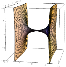
Figure 4: Surfaces defined by the same energy density. Note that there are two surfaces with the same energy for each wall. a) A vortex stretched between walls with $H_{0}(z)e^{Mx^{3}}=\sqrt{c}(e^{x^{3}},ze^{4},e^{-x^{3}})$. b) Multi-vortices between multi-walls with $H_{0}(z)e^{Mx^{3}}=\sqrt{c}((z-4-2i)(z+5+8i)e^{3/2x^{3}},(z+8-i)(z-7+6i)e^{1/2x^{3}+12},z^{2}e^{-1/2x^{3}+12},(z-6-5i)(z+6-7i)e^{-3/2x^{3}})$. c) A vortex attached to a tilted wall with $H_{0}(z)e^{Mx^{3}}=\sqrt{c}(z^{2}e^{x^{3}},e^{-1/2z})$.

Eqs. (46)–(49) determine a map from our moduli matrix $H_{0}(z)$ to all possible $1/4$ BPS solutions in three-dimensional configuration space. Therefore we find that the moduli space of the $1/4$ BPS solutions is the space of all the holomorphic maps from a complex plane to the wall moduli space, the deformed complex Grassmann manifold $G_{N_{\rm F},N_{\rm C}}={SU(N_{\rm F})\over SU(N_{\rm C})\times SU(\tilde{N}_{\rm C})\times U(1)}$ in Eq.(27).

We can obtain exact solutions in the limit of infinite gauge coupling, since the BPS equation (49) can be solved algebraically: $c\,\Omega=H_{0}\,e^{2My}H_{0}{}^{\dagger}$. To illustrate the power of our method, let us take the simplest case of $U(1)$ gauge theory with $N_{\rm F}$ flavors. The moduli vector $H_{0}(z)=\sqrt{c}\left(f^{1}(z),\,\dots,f^{N_{\rm F}}(z)\right)$ gives $\Omega=\sum_{A=1}^{N_{\rm F}}|f^{A}(z)|^{2}e^{2m_{A}x^{3}}$. Since the position of the $A$-th wall separating $A$-th and $(A+1)$-th vacua is given by $x_{A}^{3}(z)=\left(\log|f_{A+1}(z)|-\log|f_{A}(z)|\right)/(m_{A}-m_{A+1})$, $z$ dependence indicates a curved wall. Holomorphy of the moduli matrix allows only zeros or exponential dependence (entire function). If we choose zeros in the moduli matrix

$$f^{A}(z)=f^{A}_{0}\prod_{\alpha}(z-z^{A}_{\alpha})^{k^{A}_{\alpha}},\quad k^{A}_{\alpha}\in{\bf Z}_{+},$$ (50)

we obtain vortices of vorticity $k_{\alpha}^{A}$ at $z=z^{A}_{\alpha}$ in the $A$-th vacuum. A single vortex stretching between two walls is shown in Fig. 4a), where logarithmic bending of the wall is visible towards $|z|\rightarrow\infty$. We can avoid the logarithmic bending by requiring $k=\sum_{\alpha}k^{A}_{\alpha}$ to be common to walls, as illustrated in Fig. 4b). A monopole in the Higgs phase was found recently as a kink on the world volume of vortex in non-Abelian gauge theories [?]. Even in the $U(1)$ gauge theory, a similar kink occurs on the world volume of vortex. The right (left) wall separates the first (third) and the second vacua. The vortex can be regarded as a spike-like bending of the wall. Therefore there must be a transition from the first vacuum to the third vacuum when we go from right to left of the vortex. In the middle of the vortex in Fig 4a), there must be a kink, analogous to the monopole in the Higgs phase. Because of $1/g^{2}$ factor, the energy density of monopoles $t_{\rm m}$ vanish in the limit of infinite gauge coupling. The monopole charge $g^{2}t_{\rm m}$ is, however, finite as a kink on the vortex, precisely analogous to the non-Abelian case [?]. In a simple example of a vortex with winding number $k$ stretched between two walls, we obtain the monopole charge

$$\int_{V}d^{3}xg^{2}t_{\rm m}=-\pi|m_{A}-m_{B}|k.$$ (51)

Let us stress that our monopole in the Higgs phase should give non-vanishing contribution to the energy density once gauge coupling becomes finite.

If we allow an exponential function of $z$, such as $e^{mz}$, somewhere in the moduli matrix $H_{0}(z)$, the corresponding wall is no longer perpendicular to the $x^{3}$-axis. If we choose $H_{0}(z)$, for instance,

$$H_{0}e^{Mx^{3}}\!=\!\sqrt{c}(e^{m_{1}x^{3}+\tilde{m}_{1}z},\,e^{m_{2}x^{3}+\tilde{m}_{2}z}),\,\,\tilde{m}_{1,2}\in{\mathbf{C}},$$ (52)

we find that the wall position is expressed as $m_{1}x^{3}+{\rm Re}(\tilde{m}_{1}z)=$ $m_{2}x^{3}+{\rm Re}(\tilde{m}_{2}z)$. Moreover we find the magnetic field strength flows down along the tilted wall to negative infinity of $x^{3}$. If vortices are present, they are no longer perpendicular to such tilted walls as illustrated in Fig. 4c). This configuration offers a field theoretical model of the string ending on the D-brane with a magnetic flux [?].

9 Acknowledgements

The authors thank Koji Hashimoto and David Tong for a useful discussion. This work is supported in part by Grant-in-Aid for Scientific Research from the Ministry of Education, Culture, Sports, Science and Technology No.13640269 and 16028203 for the priority area “origin of mass”. K.O. and M.N. are supported by Japan Society for the Promotion of Science under the Post-doctoral Research Program. Y.I. gratefully acknowledges support from a 21st Century COE Program at Tokyo Tech “Nanometer-Scale Quantum Physics” by the Ministry of Education, Culture, Sports, Science and Technology.

References

- [1] S. Dimopoulos and H. Georgi, Nucl. Phys. B193, 150 (1981); N. Sakai, Z. f. Phys. C11, 153 (1981); E. Witten, Nucl. Phys. B188, 513 (1981); S. Dimopoulos, S. Raby and F. Wilczek, Phys. Rev. D24, 1681 (1981).
- [2] P. Horava and E. Witten, Nucl. Phys. B460, 506 (1996) [hep-th/9510209].
- [3] N. Arkani-Hamed, S. Dimopoulos and G. Dvali, Phys. Lett. B429, 263 (1998) [hep-ph/9803315]; I. Antoniadis, N. Arkani-Hamed, S. Dimopoulos and G. Dvali, Phys. Lett. B436, 257 (1998) [hep-ph/9804398].
- [4] L. Randall and R. Sundrum, Phys. Rev. Lett. 83, 3370 (1999) [hep-ph/9905221]; Phys. Rev. Lett. 83, 4690 (1999) [hep-th/9906064].
- [5] E. Witten and D. Olive, Phys. Lett. B78, 97 (1978).
- [6] M. Cvetic, F. Quevedo and S.J. Rey, Phys. Rev. Lett. 67 (1991) 1836.
- [7] G. Dvali and M. Shifman, Phys. Lett. B396, 64 (1997) [hep-th/9612128]; S. L. Dubovsky and V.A. Rubakov, Int. J. Mod. Phys. A16, 4331 (2001) [hep-ph/0105243]; M. Shifman and A. Yung, Phys. Rev. D67, 125007 (2003) [hep-th/02122293]; N. Maru and N. Sakai, Prog. Theor. Phys. 111, 907 (2004) [hep-th/0305222].
- [8] Y. Isozumi, K. Ohashi, and N. Sakai, JHEP 11, 060 (2003) [hep-th/0310189].
- [9] Y. Isozumi, K. Ohashi, and N. Sakai, JHEP 11, 061 (2003) [hep-th/0310130].
- [10] M. Shifman and A. Yung, Phys. Rev. D70, 025013 (2004) [hep-th/0312257].
- [11] Y. Isozumi, M. Nitta, K. Ohashi, and N. Sakai, Phys. Rev. Lett. to appear, [hep-th/0404198].
- [12] Y. Isozumi, M. Nitta, K. Ohashi, and N. Sakai, [hep-th/0405129].
- [13] Y. Isozumi, M. Nitta, K. Ohashi, and N. Sakai, Phys. Rev. D to appear, [hep-th/0405194].
- [14] M. Arai, M. Nitta and N. Sakai, [hep-th/0307274]; to appear in the Proceedings of the 3rd International Symposium on Quantum Theory and Symmetries (QTS3), September 10-14, 2003, [hep-th/0401084]; to appear in the Proceedings of the International Conference on “Symmetry Methods in Physics (SYM-PHYS10)” held at Yerevan, Armenia, 13-19 Aug. 2003 [hep-th/0401102]; to appear in the Proceedings of SUSY 2003 held at the University of Arizona, Tucson, AZ, June 5-10, 2003 [hep-th/0402065].
- [15] A. Hanany and D. Tong, JHEP 0307, 037 (2003) [hep-th/0306150]; M. Eto, M. Nitta, and N. Sakai, Nucl. Phys. to appear, [hep-th/0405161].
- [16] D. Tong, Phys. Rev. D69, 065003 (2004) [hep-th/0307302]; R. Auzzi, S. Bolognesi, J. Evslin, K. Konishi and A. Yung, Nucl. Phys. B673, 187 (2003) [hep-th/0307287]; R. Auzzi, S. Bolognesi, J. Evslin and K. Konishi, [hep-th/0312233]; M. Shifman and A. Yung, Phys. Rev. D70, 045004 (2004) [hep-th/0403149]; A. Hanany and D. Tong, JHEP 0404, 066 (2004) [hep-th/0403158].
- [17] J. P. Gauntlett, R. Portugues, D. Tong, and P.K. Townsend, Phys. Rev. D63, 085002 (2001) [hep-th/0008221].
- [18] E. Abraham and P. K. Townsend, Phys. Lett. B 291, 85 (1992).
- [19] D. Tong, Phys. Rev. D66, 025013 (2002) [hep-th/0202012]; D. Tong, JHEP 0304, 031 (2003) [hep-th/0303151]; J. P. Gauntlett, D. Tong and P. K. Townsend, Phys. Rev. D64, 025010 (2001) [hep-th/0012178]; M. Arai, M. Naganuma, M. Nitta, and N. Sakai, Nucl. Phys. B652, 35 (2003) [hep-th/0211103]; in Garden of Quanta - In honor of Hiroshi Ezawa, Eds. by J. Arafune et al. (World Scientific Publishing Co. Pte. Ltd. Singapore, 2003) pp 299-325, [hep-th/0302028].
- [20] K. Kakimoto and N. Sakai, Phys. Rev. D68, 065005 (2003) [hep-th/0306077].
- [21] L. Alvarez-Gaumé and D. Z. Freedman, Commun. Math. Phys. 91, 87 (1983).
- [22] J. P. Gauntlett, D. Tong, and P.K. Townsend, Phys. Rev. D63, 085001 (2001) [hep-th/0007124].
- [23] M. Naganuma, M. Nitta, and N. Sakai, Grav. Cosmol. 8, 129 (2002) [hep-th/0108133]; R. Portugues and P. K. Townsend, JHEP 0204, 039 (2002) [hep-th/0203181].
- [24] U. Lindström and M. Roček, Nucl. Phys. B222, 285 (1983); N. J. Hitchin, A. Karlhede, U. Lindström and M. Roček, Commun. Math. Phys. 108, 535 (1987).
- [25] I. Antoniadis and B. Pioline, Int. J. Mod. Phys. A12, 4907 (1997) [hep-th/9607058].
- [26] N. S. Manton, Phys. Lett. B110, 54 (1982).
- [27] K. Hashimoto, JHEP 9907, 016 (1999) [hep-th/9905162]; A. Hashimoto and K. Hashimoto, JHEP 9911, 005 (1999) [hep-th/9909202].