General Axisymmetric Solutions and Self-Tuning in 6D Chiral Gauged Supergravity

Abstract:

We re-examine the properties of the axially-symmetric solutions to chiral gauged 6D supergravity, recently found in refs. hep-th/0307238 and hep-th/0308064. Ref. hep-th/0307238 finds the most general solutions having two singularities which are maximally-symmetric in the large 4 dimensions and which are axially-symmetric in the internal dimensions. We show that not all of these solutions have purely conical singularities at the brane positions, and that not all singularities can be interpreted as being the bulk geometry sourced by neutral 3-branes. The subset of solutions for which the metric singularities are conical precisely agree with the solutions of ref. hep-th/0308064. Establishing this connection between the solutions of these two references resolves a minor conflict concerning whether or not the tensions of the resulting branes must be negative. The tensions can be both negative and positive depending on the choice of parameters. We discuss the physical interpretation of the non-conical solutions, including their significance for the proposal for using 6-dimensional self-tuning to understand the small size of the observed vacuum energy. In passing we briefly comment on a recent paper by Garriga and Porrati which criticizes the realization of self-tuning in 6D supergravity.

1 Introduction

Chiral gauged six-dimensional supergravity [1, 2] has seen considerable study for more than two decades. This has happened partly due to its sharing many of the features of ten-dimensional supergravity — and so also of string vacua — such as the existence of chiral fermions [1, 3] with nontrivial Green-Schwarz anomaly cancellation [1, 4] as well as the possibility of having chiral compactifications down to flat 4 dimensions [5]. Part of the attention has also been due to the relative simplicity of the 6D theories, which makes them comparatively simple places to explore some of the ideas [6] (such as compactifications with fluxes [7]) which have arisen in studies of 4D vacua of their higher-dimensional cousins.

More recently, interest has also come from the proposal that 6D supergravity might provide a viable example of the self-tuning of the effective 4D cosmological constant [8, 9]. The proposed self-tuning mechanism — the validity of which is still under active study — comes in two parts. The first part of the mechanism involves the cancellation of arbitrary brane tensions by the classical response of the bulk supergravity degrees of freedom, while the second part involves the size of the quantum corrections to the classical response due to bulk loops. Our discussion here is relevant for the first part of the argument. We have nothing to say in the present paper concerning the quantum part of the proposal.

Although the original claim for the classical part of this argument was based on earlier arguments from non-supersymmetric 6D theories [11], more direct conclusions have in some cases since become possible due to the subsequent discovery of a broad class of solutions to the 6D supergravity equations [12, 13]. In particular, ref. [12] find the most general solution subject to the assumptions of $(i)$ maximal symmetry in the large 4 dimensions; and $(ii)$ axial symmetry in the compact 2 dimensions. For all of the solutions within this category the intrinsic geometry of the large 4 dimensions is found to be flat.

In this note we examine further the properties of these solutions, with the immediate goal of more directly establishing the features of the metric singularities which most of these solutions have. In particular, if we interpret these singularities as being due to the gravitational back-reaction of 3-branes we wish to ascertain how the properties of the bulk field configurations are related to the properties (such as tensions) of these branes. In particular, we discuss the relevance of our results to the validity of the classical part of the self-tuning argument (in a sense we outline more concretely in what follows). In passing we resolve a minor difference between ref. [13], which allows single-brane solutions having positive tension , and v3 of ref. [12], which states all of these solutions must involve negative tension.

Our study leads to the following general conclusions:

1. The 3-parameter set of general solutions given in ref. [12] contain examples for which the metric singularities are not purely conical, and these come in two categories. Some can be interpreted as describing the fields of two localized 3-brane like objects, while others are better interpreted as the bulk fields which are sourced by a combination of a 3-brane and 4-brane, rather than being due to two 3-branes;

2. The 2-parameter subset of the general solutions of ref. [12] which have purely conical singularities can be interpreted as being sourced by two 3-branes, and these solutions precisely agree with the solutions found in ref. [13]. In particular, the tensions, $T_{\pm}$, of the two 3-branes which source all such solutions must satisfy the relation $f(T_{+},T_{-})=0$, derived in [13], and which is given explicitly by eq. (59);

3. Although topological constraints do restrict the kinds of tensions which are possible (for those solutions having only conical singularities), they need not prevent choosing both tensions to be positive if desired. This observation can be important for the analysis of the stability of these geometries.

4. We find that it is locally possible to determine the parameters of the general solution in terms of the two source brane tensions, even in the case where the singularities are not conical. This shows that a solution very likely exists for any pair of tensions, at least within a neighborhood of the conical solutions (and possibly for generic tensions). This has implications for the question of how the bulk adjusts if the tensions of the source branes are adjusted independently, as might occur for instance if a phase transition were to take place on one of the branes.

In the next section, §2, we describe the general solutions of ref. [12], and outline some of their properties. In particular we here identify the nature of their singularities. §3 is dedicated to analyzing the properties of the configurations with purely conical singularities. §4 then discusses the physical interpretation of those solutions whose singularities are more complicated than conical, and finds the tension of the source branes as functions of the parameters of the solution in the general case. In §5 we show that the subset of solutions having only conical singularities precisely agrees with those found in ref. [13], and §6 provides a discussion of the relevance of our results for the 6D self-tuning proposal. We close, in an appendix, with a brief critique of the arguments of Garriga and Porrati [10], who criticize the possibility of realizing self-tuning in 6 dimensions.

2 The Solutions of Ref. [12]

In this section we describe the general solution given in the appendix of ref. [12]. Our goal in doing so is to identify the nature of the singularities of the space-times, and to establish a baseline for the later comparison with the solutions of ref. [13].

The field content of 6D supergravity which is nonzero for these solutions consist of the 6D metric, $g_{MN}$, a 6D scalar dilaton, $\phi$ and a $U(1)$ gauge potential, $A_{M}$. The field equations which these fields must solve are

$${\hbox{$\sqcup$}\hbox to0.0pt{\hss\hbox{$\sqcap$}}}\,\phi-\frac{1}{4}\,e^{\phi/2}\;F_{MN}F^{MN}+8g^{2}e^{-\phi/2}=0$$

$$D_{M}\Bigl{(}e^{\phi/2}\,F^{MN}\Bigr{)}=0$$ (1)

$$R_{MN}-\frac{1}{4}\,\partial_{M}\phi\,\partial_{N}\phi-\frac{1}{2}\,e^{\phi/2}\,F_{MP}{F_{N}}^{P}-\frac{1}{4}\,({\hbox{$\sqcup$}\hbox to0.0pt{\hss\hbox{$\sqcap$}}}\phi)\,g_{MN}=0,$$

where $g$ is the gauge coupling constant for a specific abelian $R$-symmetry, $U(1)_{R}$, within the 6D theory.

For later purposes, we remark that these equations are invariant under the constant classical scaling symmetry,

$$g_{MN}\to\xi\,g_{MN}\qquad\hbox{and}\qquad e^{\phi/2}\to\xi\,e^{\phi/2}\,.$$ (2)

Furthermore, although the scalings $e^{\phi/2}\to\zeta^{2}\,e^{\phi/2}$ and $F_{MN}\to\zeta^{-1}\,F_{MN}$ are not a symmetry, they have the sole effect of scaling $g\to g^{\prime}=\zeta\,g$.

2.1 Solutions for General $\lambda_{3}$

Ref. [12] construct the most general solution to these equations for which 4 Lorentzian dimensions are maximally symmetric, and for which the internal 2 dimensions are axially symmetric. The metric for these solutions has at most two singularities in the extra dimensions. Their general solution is given explicitly by

$$e^{\phi} = W^{4}\,e^{2\lambda_{3}\eta}$$

$$F = {\rm d}A=\left(\frac{q\,a^{2}}{W^{2}}\,\right)e^{-\lambda_{3}\eta}\,{\rm d}\eta\wedge{\rm d}\psi$$ (3)

$${\rm d}s^{2} = W^{2}\eta_{\mu\nu}\,{\rm d}x^{\mu}{\rm d}x^{\nu}+a^{2}W^{8}{\rm d}\eta^{2}+a^{2}{\rm d}\psi^{2}\,,$$

where

$$W^{4} = \left(\frac{q\lambda_{2}}{4g\lambda_{1}}\right)\frac{\cosh\left[\lambda_{1}(\eta-\eta_{1})\right]}{\cosh\left[\lambda_{2}(\eta-\eta_{2})\right]}$$ (4)

$$a^{-4} = \left(\frac{gq^{3}}{\lambda_{1}^{3}\lambda_{2}}\right)e^{-2\lambda_{3}\eta}\cosh^{3}\left[\lambda_{1}(\eta-\eta_{1})\right]\cosh\left[\lambda_{2}(\eta-\eta_{2})\right]\,.$$ (5)

Here $q$, $\eta_{a},a=1,2$ and $\lambda_{i},i=1,2,3$ are constants, and the parameters $\lambda_{i}$ satisfy the constraint

$$\lambda_{1}^{2}+\lambda_{3}^{2}=\lambda_{2}^{2}\,.$$ (6)

Following [12] we take $\lambda_{1}$ and $\lambda_{2}$ to be positive, and so the last relation implies the inequality $\lambda_{2}\geq\lambda_{1}$.

At face value we have a total of 5 integration constants: $q$, $\lambda_{1}$, $\lambda_{2}$, $\eta_{1}$ and $\eta_{2}$. However one combination of these five constants corresponds to the scaling symmetry, eq. (2), whose action on the solution may be represented by the following transformations:

$$\psi\to\xi^{2}\psi,\quad q\to\xi^{2}q\,.$$ (7)

A second combination similarly corresponds to the second rescaling discussed above, whose sole effect is to change $g$ to $\zeta\,g$, and which for $\lambda_{3}\neq 0$ is represented on the solutions by

$$q\to\zeta\,q,\quad\eta\to\eta+\frac{2}{\lambda_{3}}\,\ln\zeta,\quad\eta_{i}\to\eta_{i}+\frac{2}{\lambda_{3}}\ln\zeta\,,$$ (8)

leaving a total of 3 nontrivial parameters. (If $\lambda_{3}=0$ then one integration constant – say $\eta_{1}$ – can similarly be removed by shifting the coordinate $\eta$ without also rescaling $q$.)

2.2 Singularities

Singularities of the metric can occur where its components vanish or diverge. Inspection of eq. (3) shows that this only occurs when $\eta\to-\infty$ and $\eta\to+\infty$. In these limits $W\propto\exp\left[\frac{1}{4}\,(\lambda_{1}-\lambda_{2})|\eta|\right]$, and so clearly $W$ remains bounded because $\lambda_{1}\leq\lambda_{2}$, and vanishes if $\lambda_{1}$ is strictly smaller than $\lambda_{2}$. Also, $a\propto\exp\left[\frac{1}{4}\,(2\lambda_{3}\eta-(3\lambda_{1}+\lambda_{2})|\eta|)\right]$ in the limit of large $|\eta|$, and so if $\pm 2\lambda_{3}+(3\lambda_{1}+\lambda_{2})$ is nonzero then $a$ either diverges or vanishes as $\eta\to\pm\infty$.

To examine the nature of the metric singularities in more detail at these points we consider the internal two-dimensional metric, which has the form ${\rm d}s^{2}_{2}=a^{2}W^{8}{\rm d}\eta^{2}+a^{2}{\rm d}\psi^{2}$. In general, in the vicinity of a conical singularity a 2D metric can always be re-written in the form

$${\rm d}s_{2}^{2}={\rm d}r^{2}+a_{0}^{2}r^{2}{\rm d}\psi^{2}$$ (9)

where $\psi$ has period $2\pi$, and the conical deficit angle at $r=0$ is given in terms of the constant $a_{0}$ by $\delta=2\pi(1-a_{0})$. We now show that this form cannot be obtained for those solutions of ref. [12] for which the parameter $\lambda_{3}$ is nonzero. The metric of the solution may be compared with this form after performing a change of variable from $\eta$ to $r$, using $aW^{4}{\rm d}\eta={\rm d}r$.

In the limit $\eta\to\pm\infty$ we have

$${\rm d}r=\frac{1}{2}\,\left(\frac{q\,e^{\mp\lambda_{1}\eta_{1}}}{\lambda_{1}}\right)^{1/4}\left(\frac{\lambda_{2}\,e^{\pm\lambda_{2}\eta_{2}}}{g}\right)^{5/4}\exp\left[-\frac{1}{4}\,(\pm 2\lambda_{3}+5\lambda_{2}-\lambda_{1})\,|\eta|\right]{\rm d}\eta\,,$$ (10)

and so the behavior of $r$ is determined by the sign of $\Delta_{\pm}\equiv\pm 2\lambda_{3}+5\lambda_{2}-\lambda_{1}$, which must be positive if $\lambda_{2}^{2}=\lambda_{1}^{2}+\lambda_{3}^{2}$. It follows that $r\to 0$ as $\eta\to\pm\infty$. As $\eta\to\pm\infty$ the metric functions $W$ and $a$ behave as $W\propto r^{\omega_{\pm}}$ and $a\propto r^{\alpha_{\pm}}$, with the powers $\alpha_{\pm}$ and $\omega_{\pm}$ satisfying the identity $\alpha_{\pm}+4\omega_{\pm}=1$, and being given explicitly by

$$\omega_{\pm}=\frac{\lambda_{2}-\lambda_{1}}{\Delta_{\pm}}\,,\qquad\qquad\alpha_{\pm}=\frac{\pm 2\lambda_{3}+\lambda_{2}+3\lambda_{1}}{\Delta_{\pm}}\,.$$ (11)

Notice that in the special case $\lambda_{1}=\lambda_{2}\equiv\lambda$, we have $\lambda_{3}=0$ and so $\omega_{\pm}=0$ and $\alpha_{\pm}=1$.

We now turn to the asymptotic behavior of the functions $W$ and $a$ as $r\to 0$. As mentioned previously, the inequality $\lambda_{2}\geq\lambda_{1}$ implies $\omega_{\pm}\geq 0$ and so (unless $\lambda_{1}=\lambda_{2}$) $W$ vanishes at both singularities. The behavior of $a$ near the singularities is similarly controlled by the power $\alpha_{\pm}$. For instance, $\alpha_{+}=0$ can happen for positive $\lambda_{1}$ and $\lambda_{2}$ only when $\lambda_{3}=2\lambda_{1}[-1-1/\sqrt{3}]<0$ and $\lambda_{2}=\lambda_{1}[1+4/\sqrt{3}]>0$. Similarly, $\alpha_{-}=0$ requires $\lambda_{3}=2\lambda_{1}[1+1/\sqrt{3}]>0$ and $\lambda_{2}=\lambda_{1}[1+4/\sqrt{3}]>0$. Thus, the inequalities $\alpha_{+}<0$ and $\alpha_{-}<0$ describe the two wedges in the upper-half $\lambda_{1}-\lambda_{3}$ plane illustrated in Fig. (1). It is clear from this that it is possible to choose non-negative $\lambda_{1}$ and $\lambda_{2}$ to ensure one of two possibilities: ($i$) $\alpha_{\pm}$ both positive; or ($ii$) $\alpha_{\pm}$ have opposite sign. It is not possible for both $\alpha_{\pm}$ to be negative, and both can vanish only if $\lambda_{1}=\lambda_{2}=0$.

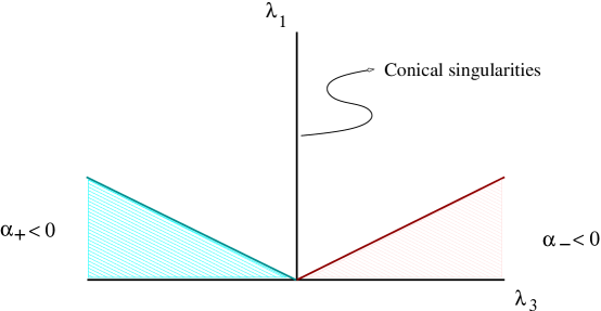
Figure 1: Solid regions indicate where in the $\lambda_{1}-\lambda_{3}$ plane, the powers $\alpha_{\pm}$ are negative. Notice the existence of a big region for which both $\alpha_{\pm}>0$. Only for $\lambda_{3}=0$ are the singularities conical.

With these results we see that the angular part of the metric near the singularities becomes $a^{2}{\rm d}\psi^{2}\to a^{2}_{\pm}\,r^{2\alpha_{\pm}}\,{\rm d}\psi^{2}$, where $a_{\pm}$ is a constant. In the special case $\lambda_{3}=0$ (and so also $\lambda_{1}=\lambda_{2}\equiv\lambda$) we have $\alpha_{\pm}=1$ and $\omega_{\pm}=0$, and so the metric takes a conical form with defect parameter $a_{\pm}=\lambda(4g/q)e^{\pm\lambda(\eta_{1}-\eta_{2})}$ (corresponding to the defect angle $\delta_{\pm}=2\pi(1-a_{\pm})$). For any other $\alpha_{\pm}$ the 2D metric cannot be brought into the conical-defect form near the singularity, and so the metric here is not locally a cone.

Notice also that so long as $\alpha\neq 1$ local bulk-curvature invariants diverge in the limit $r\to 0$ (by contrast with the delta-function behavior which obtains in the case of a conical singularity). A similar statement also holds for the bulk dilaton and electromagnetic fields, which can diverge or vanish at the positions of the branes depending on the particular values chosen for $\lambda_{1}$ and $\lambda_{2}$. We further discuss the interpretation of the singularities when $\alpha_{\pm}\neq 1$ in §3, below.

3 The Special Case $\lambda_{3}=0$

In this section, we analyze the properties of general GGP solutions for the special case $\lambda_{3}=0$, for which the above discussion shows that the metric singularities are conical. Because the parameters $\lambda_{1}$ and $\lambda_{2}$ are positive and satisfy the relation (6), we must in this case also choose $\lambda_{1}=\lambda_{2}=\lambda$. We shall see that in the particular case $\lambda=1$, one of the conical singularities disappears, leaving only a single singularity. This is the case considered in Section 2 of ref. [12].

3.1 The Solution

When $\lambda_{3}=0$ and $\lambda_{1}=\lambda_{2}=\lambda$ the general solution reduces to

$$e^{\phi} = W^{4}$$

$$F = \left(\frac{q\,a^{2}}{W^{2}}\right)\,{\rm d}\eta\wedge{\rm d}\psi$$ (12)

$${\rm d}s^{2} = e^{{\phi}/{2}}\eta_{\mu\nu}\,{\rm d}x^{\mu}{\rm d}x^{\nu}+a^{2}W^{8}{\rm d}\eta^{2}+a^{2}{\rm d}\psi^{2}\,,$$

where

$$W^{4} = \left(\frac{q}{4g}\right)\frac{\cosh\left[\lambda(\eta-\eta_{1})\right]}{\cosh\left[\lambda(\eta-\eta_{2})\right]}$$ (13)

$$a^{-4} = \left(\frac{gq^{3}}{\lambda^{4}}\right)\cosh^{3}\left[\lambda(\eta-\eta_{1})\right]\cosh\left[\lambda(\eta-\eta_{2})\right]\,.$$ (14)

We are left with the 4 integration constants, $q$, $\lambda$, $\eta_{1}$ and $\eta_{2}$, and one of $\eta_{1}$ or $\eta_{2}$ can be removed by appropriately shifting $\eta$. As previously discussed the scale invariance, (2), is implemented by $q\to\xi^{2}\,q$ and $\psi\to\xi^{2}\,\psi$. The authors of ref. [12] remove this classical symmetry by using it to impose the condition

$$e^{\lambda(\eta_{1}-\eta_{2})}=\frac{r_{1}}{r_{0}}\,\,,$$ (15)

where the $r_{i}$ are given by

$$r_{0}^{2}=\frac{1}{2g^{2}}\,\hskip 14.22636pt,\hskip 14.22636ptr_{1}^{2}=\frac{8}{q^{2}}\,.$$ (16)

This choice, and the freedom to shift $\eta$, reduces the number of integration constants to two.

At this point, it is useful to define a new radial coordinate $0\leq\sigma<\infty$, by:

$$\sigma=r_{1}e^{\lambda(\eta-\eta_{1})}\,,$$ (17)

in which case the solution, eq. (12), becomes

$$\phi = \ln\left({\frac{f_{1}}{f_{0}}}\right)$$

$$F = \left(\frac{q\lambda\,\sigma}{f_{1}^{2}}\right)\,{\rm d}\sigma\wedge{\rm d}\psi$$ (18)

$${\rm d}s_{6}^{2} = \left(\frac{f_{1}}{f_{0}}\right)^{{1}/{2}}\left(\eta_{\mu\nu}\,{\rm d}x^{\mu}{\rm d}x^{\nu}\right)+\left(\frac{f_{1}}{f_{0}}\right)^{{1}/{2}}\left(\frac{{\rm d}\sigma^{2}}{f_{0}^{2}}+\frac{\lambda^{2}\sigma^{2}}{f_{1}^{2}}\,{\rm d}\psi^{2}\right)\,,$$

where

$$f_{0}\equiv 1+\frac{\sigma^{2}}{r_{0}^{2}}\hskip 28.45274pt\hbox{and}\hskip 28.45274ptf_{1}\equiv 1+\frac{\sigma^{2}}{r_{1}^{2}}\,.$$ (19)

We see that in this form the solution explicitly depends only on the two independent integration constants, which we may take to be $q$ and $\lambda$.

Analyzing the metric of eq. (18), it is easy to see that for $\lambda\neq 1$ there are two conical singularities, one at $\sigma=0$ and the other at $\sigma=+\infty$. The corresponding deficit angles are given by

$$\frac{\delta_{0}}{2\pi}=1-\lambda\hskip 56.9055pt\frac{\delta_{\infty}}{2\pi}=1-\lambda\left(\frac{r_{1}^{2}}{r_{0}^{2}}\right)\,.$$ (20)

As is clear from these expressions, the conical singularity at the origin disappears when $\lambda=1$. The tensions of the branes at the conical singularities may be read off from these expressions, since they are proportional to the deficit angles:

$$T=\frac{\delta}{8\pi G}\,,$$ (21)

where we briefly reinstate the 6D Newton constant, $8\pi G=\kappa^{2}$.

3.2 Topological Constraints

In this subsection, we re-examine the topological constraints that the previous solution must satisfy. Our discussion here, which generalizes the topological constraints discussed for the simplest unwarped solution in refs. [8, 15] (see also [16]), follows the method presented in [12]. Our interest is mainly to investigate the consequences of this constraint for the sign of the brane tensions.

To this end we notice that the field strength $F$ of the solution, eq. (18), locally can be written in terms of the one-form potential

$$A=-\left(\frac{4\lambda}{qf_{1}}\right){\rm d}\psi\,.$$ (22)

In order for this section of the gauge bundle to be globally well-behaved it is necessary to impose the quantization condition

$$\frac{4\lambda\,\tilde{g}}{q}=N\,,$$ (23)

where $N$ an integer and $\tilde{g}$ is the 6D gauge coupling for the particular gauge field which is nonzero in the classical solution. Notice that by writing only one quantization condition we assume the background $U(1)$ to lie completely within a simple factor of the gauge group for which there is only a single gauge coupling. Even so, in general $\tilde{g}$ need not equal the coupling, $g$, appearing in the dilaton potential since the field strength which is turned on in the classical solution need not be for the specific $U(1)_{R}$ generator whose coupling is $g$.

The Special Case $g=\tilde{g}$.

If we do take $g=\tilde{g}$ — such as we must if the background gauge field gauges the $U(1)_{R}$ symmetry of 6D chiral supergravity — it is immediate that at least one of the brane tensions must be negative so long as $N\neq 0$ [12]. To see this we use the quantization result, (23), in the form

$$\frac{r_{1}}{r_{0}}=\frac{4g}{q}=\frac{N}{\lambda}\,,$$ (24)

to see that the deficit angles become

$$\frac{\delta_{0}}{2\pi}=1-\lambda\hskip 28.45274pt\hbox{and}\hskip 28.45274pt\frac{\delta_{\infty}}{2\pi}=1-\frac{N^{2}}{\lambda}\,.$$ (25)

From these expressions it is easy to see that at least one of the branes must have negative tension, since $\lambda$ is positive and $N^{2}\geq 1$.

An interesting particular case of this situation is obtained by specializing to the rugby-ball geometry, for which the two tensions are equal [8, 15]. Using eq. (20) we see this corresponds to the special case $r_{1}=r_{0}$, for which the following change of radial variable

$$\sigma=r_{0}\tan{\frac{\theta}{2}}\,,$$ (26)

allows the metric for the two internal dimensions, taken from the solution eq. (18), to be rewritten as

$${\rm d}s_{2}^{2}\equiv\left(\frac{f_{1}}{f_{0}}\right)^{{1}/{2}}\left(\frac{{\rm d}\sigma^{2}}{f_{0}^{2}}+\frac{\lambda^{2}\sigma^{2}}{f_{1}^{2}}\,{\rm d}\psi^{2}\right)=\frac{r_{0}^{2}}{4}\left({\rm d}\theta^{2}+\lambda^{2}\sin^{2}{\theta}\,{\rm d}\psi^{2}\right)\,.$$ (27)

From this form of the metric it is immediate to see that the geometry being described is a sphere with deficit angle $\delta=2\pi(1-\lambda)$ removed at each of the poles. For this metric the quantization condition, eq. (24), implies $\lambda=N$, and so the deficit angle $\delta$ of the two conical singularities is given by

$$\frac{\delta}{2\pi}=1-N\,.$$ (28)

Again the tensions are negative for any nonzero integer $N$.

The Case $g\neq\tilde{g}$.

Situations having positive tension may be found by taking $g<\tilde{g}$, in which case the quantization condition, (23), implies

$$\frac{r_{1}}{r_{0}}=\frac{Ng}{\lambda\tilde{g}}\,\,.$$ (29)

This leads to the following expressions for the deficit angles:

$$\frac{\delta_{0}}{2\pi}=1-\lambda\hskip 56.9055pt\frac{\delta_{\infty}}{2\pi}=1-\frac{N^{2}}{\lambda}\left(\frac{g}{\tilde{g}}\right)^{2}\,.$$ (30)

Clearly, both the brane tensions can be positive in this case provided $\lambda<1$ and $(g/\tilde{g})^{2}<\lambda/N^{2}$. In the particular case of the rugby-ball geometry, one finds that the deficit angle becomes

$$\frac{\delta}{2\pi}=1-\frac{Ng}{\tilde{g}}\,,$$ (31)

which can again be positive if $g/\tilde{g}<1/N$.

Superficially, the above expressions seem to disagree with the conclusion drawn in version 3 of ref. [12], wherein it is claimed that one of the tensions must be negative for any of the solutions having only one singularity. This contradiction is only superficial because GGP draw this conclusion under the assumption that the gauge field turned on in the background is a nontrivial mixture of two gauge directions for which the couplings are different. They do so by taking it to be a linear combination of an internal gauge group (such as one which commutes with supersymmetry) and of the specific $U(1)_{R}$ gauge group whose gauge coupling, $g$, appears in the dilaton potential. As is clear from their expressions, the requirement for negative tension disappears if the background field is purely orthogonal to the $U(1)_{R}$ direction, since in this case only one of their two quantization conditions applies and is in itself insufficient to force one of the tensions to be negative.

For later convenience we pause to record a relation between the tensions which always holds when $\lambda_{3}=0$, and which is obtained from eqs. (30) by eliminating the common variable $\lambda$ and using the relation (21), $\delta=8\pi G\,T$:

$$(1-4G\,T_{0})(1-4G\,T_{\infty})=N^{2}\left(\frac{g^{2}}{\tilde{g}^{2}}\right)\,.$$ (32)

This expression generalizes the relation derived in ref. [12] to the case $\tilde{g}\neq g$.

4 The Branes Behind the Solutions

The existence of solutions having non-conical metric singularities (when $\lambda_{3}\neq 0$) raises several interpretational issues, if these singularities are to be interpreted as the positions of various branes whose stress-energy and charges source these bulk fields. In order to better understand what is going on, it is useful to consider the behavior of the fields in the vicinity of a single brane for pure gravity (without the dilaton and electromagnetic fields).

4.1 Singular Single-Brane Configurations

Consider therefore pure gravity in 6 dimensions (which also applies to 6D supergravity in the limit $g=0$), with the metric chosen to have the general axially-symmetric form

$${\rm d}s^{2}=W^{2}(r)\,\eta_{\mu\nu}\,{\rm d}x^{\mu}{\rm d}x^{\nu}+{\rm d}r^{2}+A^{2}(r)\,{\rm d}\theta^{2}\,.$$ (33)

A simple calculation shows that the condition that this metric be a vacuum spacetime — i.e. one satisfying $R_{MN}=\frac{1}{2}\,R\,g_{MN}$ — has two types of solutions.

1. The first class of solution is the usual unwarped cone, for which $W(r)=W_{0}$ and $A(r)=A_{0}\,r$, with $W_{0}$ and $A_{0}$ being arbitrary positive constants.

2. The second class of solution has $W(r)=W_{0}r^{2/5}$ and $A(r)=A_{0}r^{-3/5}$, where $A_{0}$ and $W_{0}$ are again the integration constants. Unlike the conical metrics, these warped solutions are not locally flat geometries.

We see in this way the existence of non-conical warped solutions which are not asymptotically locally-flat, just as for the more general $\lambda_{3}\neq 0$ GGP solutions. In both Einstein gravity and the GGP solutions the local curvature invariants diverge as one approaches the brane position, as opposed to the simple delta-function behavior which arises for the conical singularities. Other bulk fields, like the dilaton and Maxwell fields, can also blow up or vanish at these points depending on the values chosen for $\lambda_{1}$ and $\lambda_{2}$.

The existence of this second type of solution to the Einstein equations has also been noticed for 4 dimensions in the context of the gravitational field produced by cosmic strings. However it was initially discarded on the grounds that it was inappropriate to the desired cosmic-string applications [17]. More recently it has been re-examined for its possible relevance to super-massive or global-string configurations [18]. Similar single-brane solutions (involving different powers of $r$ in $W$ and $a$) also exist for the coupled dilaton-Einstein system, for instance with the result in 4 dimensions being given in ref. [19].

4.2 Interpretational Issues

In any case, which of these solutions is appropriate in a given physical situation is determined in principle by a set of boundary conditions at the brane positions. To this end, suppose the source brane is not regarded to be arbitrarily thin and is instead resolved to have a small proper width, $\ell$, within which some new stress-energy turns on and smooths out the singular geometry at $r=0$. Then it is the matching of this smooth geometry internal to the brane with the external geometry which decides which external solution is appropriate. This kind of matching has been done explicitly for weakly-gravitating local cosmic strings [22], subject to suitable falloff conditions for the interior energy density, with the result that these kinds of objects choose the asymptotically conical solutions. We now re-examine this matching within Einstein gravity for more general strongly-coupled sources.

To do so suppose that the exterior metric of (33) applies for $r\geq\ell$, and smoothly matches onto a regular geometry for $0\leq r\leq\ell$ of the same form

$${\rm d}s^{2}={{\cal W}}^{2}(r)\,\eta_{\mu\nu}\,{\rm d}x^{\mu}{\rm d}x^{\nu}+{\rm d}r^{2}+{{\cal A}}^{2}(r)\,{\rm d}\theta^{2}\,,$$ (34)

since we again demand maximal symmetry for the infinite 4 dimensions. The explicit form of the coefficients ${\cal W}$ and ${\cal A}$ depends on the internal stress energy which resolves the structure of the brane for $r\leq\ell$. Requiring the interior metric to be well defined at the origin implies

$${\cal W}(0)=1\,,\qquad{\cal W}^{\prime}(0)=0\hskip 28.45274pt\hbox{and}\hskip 28.45274pt{\cal A}(0)=0\,,\qquad{\cal A}^{\prime}(0)=1\,,$$ (35)

and the condition that it smoothly connect with the exterior metric at $r=\ell$ implies:

$${\cal W}(\ell)=W(\ell)\approx\,W_{0}\,\ell^{\omega}\,,\quad\,\,{\cal W}^{\prime}(\ell)=W^{\prime}(\ell)\approx\omega\,W_{0}\,\ell^{\omega-1}$$

$${\cal A}(\ell)=A(\ell)\approx A_{0}\,\ell^{\alpha}\,,\qquad{\cal A}^{\prime}(\ell)=A^{\prime}(\ell)\approx\alpha\,A_{0}\,\ell^{\alpha-1}\,\,,$$ (36)

for some constants $W_{0}$, $A_{0}$, $\alpha$ and $\omega$.

There are two separate kinds of interpretational issues which this kind of matching raises: Are the sources 3-branes or 4-branes? And: If they are 3-branes how are their brane properties related to the kind of external solution which is appropriate? We address each of these in turn in the remainder of this section.

3-Branes vs 4-Branes

In order for the source to be interpreted as a 3-brane, its proper transverse size must be small compared with those of the exterior space. Although this is generally true for the brane’s proper radius, since by definition $r>\ell$ for all points exterior to the brane, in order to interpret the source as a 3-brane we also demand it to be true for the brane’s circumference, $C_{b}=2\pi A(\ell)$, relative to the circumference of circles, $C(r)=2\pi A(r)$, which surround the brane at some proper separation $r$. (We could equivalently phrase this criterion in terms of the transverse volume of the brane, $\Omega_{\ell}=\int_{0}^{\ell}dx\,{\cal A}(x)$, relative to the volume interior to various circles which surround the brane, $\Omega(r)=\Omega_{\ell}+\int_{\ell}^{r}dx\,A(x)$.)

Clearly, if $\alpha>0$ then $A$ increases as $r$ increases and so the circumference, $A(\ell)$, at the brane boundary is smaller than the circumference of those circles which surround the brane at radii $r>\ell$. This is what would be expected for a 3-brane whose size is much smaller than the size of the bulk geometry within which it sits. The opposite situation arises if $\alpha<0$, since then $A(r)$ is a decreasing function as $r$ increases. In this case the external geometry resembles that of the mouth of a trumpet, with the circumference, $A(\ell)$, of the circle at the boundary of the brane being in this case larger than the circumference of all of the circles which surround the brane at $r>\ell$. In this case the source brane is hard to interpret as a point source within a larger bulk, and the bulk geometry, (33), is better interpreted as being sourced by a 4-brane than by a 3-brane.

For the single-brane solutions given by eq. (33), the choices are $\alpha=1$ or $\alpha=-3/5$, and so it is only those geometries having conical singularities which would be interpreted as being sourced by localized 3-branes according to the above interpretation. The same is not true for the GGP solutions, for which we have seen that $\alpha$ can be positive but not equal to unity, and so furnish examples of geometries with non-conical singularities for which $A(r)$ is an increasing function of $r$. This possibility relies for its existence on the presence of the dilaton in the bulk.

The very existence of these geometries raises the possibility that there may be localized 3-brane sources for which the external metric does not simply have the usual conical singularity. We now try to ascertain precisely what properties of the brane, besides its tension, dictate when and whether the external geometry can be singular in this way.

4.3 Smoothing Out 3-Branes

To see what kinds of brane properties control the form of the external metric, we specialize the above considerations to the asymptotic forms obtained earlier for the singular GGP solutions (i.e. those having $\lambda_{3}$ nonzero). As discussed in §2 above, the change of variables (10) allows us in this case to explicitly compute the constants $A_{\pm}$, $W_{\pm}$, $\omega_{\pm}$ and $\alpha_{\pm}$ defined by $W=W_{\pm}r^{\omega_{\pm}}$ and $A=A_{\pm}r^{\alpha_{\pm}}$. In the present case, near the singularities at $\eta\to\pm\infty$ we have

$$W_{\pm}^{2} = \left(\frac{q\,\lambda_{2}}{4g\,\lambda_{1}}\right)^{\frac{1}{2}}e^{\mp(\lambda_{1}\eta_{1}-\lambda_{2}\eta_{2})/2}\,\left[\frac{\Delta_{\pm}^{2}}{4}\left(\frac{\lambda_{1}\,e^{\pm\lambda_{1}\eta_{1}}}{q}\right)^{\frac{1}{2}}\left(\frac{g\,e^{\mp\lambda_{2}\eta_{2}}}{\lambda_{2}}\right)^{5/2}\right]^{\omega_{\pm}}$$ (37)

$$A_{\pm}^{2} = 4\left(\frac{\lambda_{1}^{3}\lambda_{2}}{g\,q^{3}}\right)^{1/2}e^{\pm(3\lambda_{1}\eta_{1}+\lambda_{2}\eta_{2})/2}\left[\frac{\Delta_{\pm}^{2}}{4}\left(\frac{\lambda_{1}\,e^{\pm\lambda_{1}\eta_{1}}}{q}\right)^{\frac{1}{2}}\left(\frac{g\,e^{\mp\lambda_{2}\eta_{2}}}{\lambda_{2}}\right)^{5/2}\right]^{\alpha_{\pm}}\,,$$ (38)

while the exponents $\omega_{\pm}$ and $\alpha_{\pm}$ are given by eq. (11), which we reproduce here for convenience:

$$\omega_{\pm}=\frac{\lambda_{2}-\lambda_{1}}{5\lambda_{2}-\lambda_{1}\pm 2\lambda_{3}}\qquad\hbox{and}\qquad\alpha_{\pm}=\frac{\lambda_{2}+3\lambda_{1}\pm 2\lambda_{3}}{5\lambda_{2}-\lambda_{1}\pm 2\lambda_{3}}\,.$$ (39)

and $\Delta_{\pm}=5\lambda_{2}-\lambda_{1}\pm 2\lambda_{3}$. Recall also that $\alpha_{\pm}$ and $\omega_{\pm}$ satisfy the identity $\alpha_{\pm}+4\omega_{\pm}=1$. As discussed earlier, in the limiting case $\lambda_{1}=\lambda_{2}=\lambda$ (and so $\lambda_{3}=0$) these reduce to the case of a conical singularity, for which

$$W_{\pm}=1\,,\hskip 28.45274pt\omega_{\pm}=0\,,\hskip 28.45274ptA_{\pm}=\lambda\,,\hskip 28.45274pt\alpha_{\pm}=1\,\,,$$ (40)

but for $\lambda_{3}\neq 0$, the metric has a more complicated curvature singularity at $r=0$.

Consider now the stress-energy which is responsible for smoothing out the brane. We take for these purposes an internal energy-momentum tensor having the most general rotationally-invariant form

$${T^{M}}_{\,N}=-\hbox{diag}\left(\epsilon,\epsilon,\epsilon,\epsilon,p,\sigma\right)\,,$$ (41)

where the functions $\epsilon(r)$, $p(r)$ and $\sigma(r)$ vanish for $r>\ell$. We ask these to be related to the internal-metric functions, ${\cal W}(r)$ and ${\cal A}(r)$, through the interior Einstein equations, $G_{MN}=8\pi G\,T_{MN}$, where we imagine here that $T_{MN}$ also includes the energy-momentum of the bulk dilaton and the gauge field within the brane.

The above expressions allow us to draw some preliminary conclusions about the connection between the external geometry and brane properties. For example, Einstein’s equations allow us to write the following expression for the brane tension

$$T_{\ell_{\pm}} = \int_{0}^{2\pi}{\rm d}\theta\int_{0}^{\ell}{\rm d}r\,\sqrt{-{g}_{6}}\;\epsilon=-\frac{1}{8\pi G}\int_{0}^{2\pi}{\rm d}\theta\int_{0}^{\ell}{\rm d}r\,{\cal W}^{4}(r)\,{\cal A}(r){G^{t}}_{t}$$

$$= -\frac{1}{8\pi G}\int_{0}^{2\pi}{\rm d}\theta\int_{0}^{\ell}{\rm d}r\,{\cal W}^{2}\,[3\,{\cal W}^{\prime 2}{\cal A}+3\,{\cal W}\,{\cal W}^{\prime}{\cal A}^{\prime}+3\,{\cal W}\,{\cal W}^{\prime\prime}{\cal A}+{\cal W}^{2}{\cal A}^{\prime\prime}]$$

$$= \frac{2\pi}{8\pi G}\left[1-A_{\pm}\,W_{\pm}^{4}\ell^{4\omega+\alpha-1}(\alpha_{\pm}+3\omega_{\pm})\right]+\frac{2\pi}{8\pi G}\left(4\int_{0}^{\ell}{\cal W}^{3}{\cal W}^{\prime}{\cal A}^{\prime}\,{\rm d}r+6\,\int_{0}^{\ell}{\cal W}^{2}\,({\cal W}^{\prime})^{2}\,{\cal A}\,{\rm d}r\right)$$

$$= \frac{2\pi}{8\pi G}\left[1-A_{\pm}\,W_{\pm}^{4}(\alpha_{\pm}+3\omega_{\pm})\right]+\frac{2\pi}{8\pi G}\left(4\int_{0}^{\ell}{\cal W}^{3}{\cal W}^{\prime}{\cal A}^{\prime}\,{\rm d}r+6\,\int_{0}^{\ell}{\cal W}^{2}\,({\cal W}^{\prime})^{2}\,{\cal A}\,{\rm d}r\right)\,,$$ (43)

where we have used the boundary conditions (4.2) with $W_{0}=W_{\pm}$, $A_{0}=A_{\pm}$, $\alpha=\alpha_{\pm}$ and $\omega=\omega_{\pm}$, corresponding to the constants associated with the singularities at $\eta\to\pm\infty$ to evaluate the integrals. The last line uses the identity $\alpha_{\pm}+4\omega_{\pm}=1$. Notice that the integrals in the last line of this expression tend to zero in the limit $\ell\to 0$, provided that the metric functions ${\cal W}$ and ${\cal A}$ are nonsingular and sufficiently well behaved throughout the integration range $0<r<\ell$. Consequently we find the following general relation between the tensions, $T_{\pm}$, and the parameters which govern the asymptotic form of the external metric:

$$T_{\pm}=\lim_{\ell\to 0}T_{\ell_{\pm}}=\frac{1}{4G}\left[1-A_{\pm}\,W_{\pm}^{4}\left(\alpha_{\pm}\,+3\omega_{\pm}\right)\right]\,.$$ (44)

If we use the explicit expressions given earlier for $A_{\pm}$, $W_{\pm}$, $\alpha_{\pm}$ and $\omega_{\pm}$ as functions of the parameters $\lambda_{1}$, $\lambda_{2}$, $q$, etc. into these expressions for the tensions, then we see that eq. (44) shows how to relate the brane tensions to the parameters appearing in the bulk solutions, even for the non-conical geometries. As is easily verified, it reduces in the case of conical singularities to the standard connection between the tension and defect angle, since in this case inserting formulae (40) into (43) gives for the $\eta\to-\infty$ singularity

$$T=\frac{1}{4G}(1-\lambda)\,.$$ (45)

We learn from this that the tension in itself is insufficient to determine both of the powers $\alpha$ and $\omega$. So what is it which determines whether the external geometry is unwarped and conical or warped and more singular? A clue to this comes from the $\theta-\theta$ components of the Einstein equations, which read ${G^{\theta}}_{\theta}=8\pi G\,{T^{\theta}}_{\theta}$, or

$$10\left(\frac{d}{dr}\ln{\cal W}\right)^{2}+4\frac{d^{2}}{dr^{2}}\ln{\cal W}=8\pi G\,\sigma\,,$$ (46)

since this shows that a constant warp factor external to the brane, $W^{\prime}(\ell)={\cal W}^{\prime}(\ell)=0$, is only possible if $\sigma={T^{\theta}}_{\theta}$ also vanishes at $r=\ell$. For instance $\sigma$ might be nonzero due to the microscopic stress which resolves the brane, or it could be nonzero because of the presence near the brane of nontrivial dilaton or electromagnetic fields. Clearly conical geometries must lie external to ‘thin wire’ branes for which ${T^{\mu}}_{\nu}=T\delta^{2}(x)\,{\delta^{\mu}}_{\nu}$ and ${T^{r}}_{r}={T^{\theta}}_{\theta}=0$, but it is the absence of transverse stress-energy which is responsible for this fact.

In general, the small-$\ell$ limit is a singular one which depends on the details of the microscopic physics which smooths out the brane in question. However, general physical arguments (see for instance [24, 25]) ensure that for small $\ell$ it is always possible to organize this dependence into an effective action localized at the brane positions, with successive higher-dimension terms suppressed by higher powers of $\ell$. For instance, we speculate that it may be the appearance of effective operators involving the normal components of the curvatures (such as $R_{ij}=n_{i}^{M}n_{i}^{M}\,R_{MN}$, with $n_{i}^{M},i=1,2$ denoting unit normals to the 3-brane) within the localized brane action which would reflect in this way the presence of non-zero $\sigma(\ell)$. It would be of considerable practical interest to pin down this issue, by finding the detailed matching between the properties of the microscopic stress-energy profiles, $\epsilon$, $p$ and $\sigma$, used above, and the corresponding effective operators in the brane effective action.

5 The Solutions of Ref. [13].

This section is dedicated to demonstrate the equivalence between the solutions of ref. [13] and the solution of eq. (18): that is, the general solution of ref. [12] having two or fewer singularities that are conical. We do so in order to clarify how the solutions of these two references are related to one another.

5.1 The Solutions and Their Relation to Those of Ref. [12]

This equivalence is proven by explicitly constructing the coordinate transformation which relates the two solutions. The solutions constructed in ref. [13] are given by 

$${\rm d}s_{6}^{2}=2\,r[-{\rm d}t^{2}+{\rm d}x_{3}^{2}]+h(r)\,{\rm d}\psi^{2}+\frac{{\rm d}r^{2}}{h(r)}\equiv e^{{\phi}/{2}}\eta_{\mu\nu}\,{\rm d}x^{\mu}{\rm d}x^{\nu}\,+\,{\rm d}s_{2}^{2}\,,$$ (47)

$$\phi(r)=2\ln(2r)+\phi_{0}\,,$$ (48)

$$F=\frac{\tilde{q}\,e^{-{\phi_{0}}/{4}}}{8\,r^{3}}\,\,{\rm d}r\wedge{\rm d}\psi\,,$$ (49)

with

$$h(r)=\frac{2m}{r}-\,g^{2}\,e^{-{\phi_{0}}/{2}}\,r-\,\frac{\tilde{q}^{2}}{256\,r^{3}}\,.$$ (50)

To obtain these expressions we take the solutions of ref. [13] and make the replacements $\phi\to-\phi/2$ as well as re-scaling our units for the 6D Planck scale from $\kappa^{2}=1$ to $\kappa^{2}=\frac{1}{2}$, as is required in order to conform with the conventions used here and in ref. [12]. We also must take $R_{MN}\to-R_{MN}$ in order to change from the Weinberg curvature convention used in [13] to the MTW conventions of [12]. Finally, we also re-name the integration constant ${\cal A}$ of ref. [13] to $\tilde{q}$, according to $8{\mathcal{A}}=\tilde{q}$. As written, this solution has 3 integration constants, $\phi_{0}$, $\tilde{q}$ and $m$, which is the same counting (before fixing the classical scale invariance) as for the $\lambda_{3}=0$ solutions discussed above.

In order to show the equivalence of this solution with that of eq. (18), it is enough to change the radial coordinate $r$ in the solution (47, 48, 49), to a new coordinate $\eta$ via the relation

$$2\,r\,e^{{\phi_{0}}/{2}}=\,W^{2}(\eta)$$ (51)

where the function $W(\eta)$ is the one given in formula (13). From here, it is clear that the scalar $\phi$ of eq. (48) matches the scalar of eq. (3) in the solution of [12]. Using this definition of $\eta$ leads to the following formula

$${\rm d}\,r=e^{-\phi_{0}/2}\frac{\lambda W^{2}}{4}\Big{\{}\tanh{[\lambda\left(\eta-\eta_{1}\right)]}-\tanh{[\lambda\left(\eta-\eta_{2}\right)]}\Big{\}}\,{\rm d}\,\eta\,.$$ (52)

At this point, we match the integration constants of the solution in [13] with the integration constants of the solution in [12]. In particular, we must re-write the integration constants $q$ and $\lambda$ of the solution in section (3) in terms of the integration constants given here by

$$\tilde{q}^{2}=q^{2}\,e^{-{5\phi_{0}}/{2}}\,,$$ (53)

and we set

$$\frac{1}{\lambda}\sinh{[\lambda(\eta_{2}-\eta_{1})]} = \frac{2\,e^{{\phi_{0}}/{2}}}{gq}\,\,,$$

$$\cosh{[\lambda(\eta_{2}-\eta_{1})]} = \frac{16m\,e^{{3\phi_{0}}/{2}}}{gq}\,.$$

Substituting the definition of $r$ in terms of $\eta$, given in (51), into the solutions (47, 48, 49, 50), and using the conditions (LABEL:condrel), it is straightforward to show that one obtains in this way the solution discussed in §3.

Notice that the change of variables defined by eq. (51) is only locally well-defined. This is because it defines $r$ to be a double-valued function of the coordinate $\eta$, since $W$ increases as one moves away from the brane at $\eta\to-\infty$ and then decreases again as the other brane is approached as $\eta\to+\infty$. In particular, the special case of the unwarped rugby-ball solutions can only be obtained from the warped solutions of this section through an appropriate limiting procedure – as we show in detail below. This limiting procedure is required because in the special case of the unwarped rugby-ball solutions the change of variables (51) is singular, since for these solutions $W$ is a constant.

This establishes the equivalence of the solutions of ref. [13] with those solutions of ref. [12] for which $\lambda_{3}=0$. The integration constants, $q$, $\lambda$ and $\eta_{1}-\eta_{2}$ of one solution are interchangeable for the integration constants, $m$, $\tilde{q}$, and $\phi_{0}$ of the other. In particular, the choice $\lambda=1$ which produces a solution having only a single conical singularity corresponds to adjusting the choice of the parameter $m$ in terms of $\tilde{q}$ and $\phi_{0}$ in such a way as to make one of the tensions vanish.

5.2 Topological Constraints

Having established the connection between the solutions of the two papers, it is possible to use directly the results of ref. [13] to infer which brane properties are consistent with the constraints, such as those from topology. Physically, we are in principle free to choose the tensions, $T_{\pm}$, of each of the source branes as well as choose the total monopole number, $N$, of the background magnetic flux. The topological constraint, eq. (23), in terms of the coordinates in ref. [13], reads

$$\frac{\tilde{q}}{32}\left(\frac{1}{r_{-}^{2}}-\frac{1}{r_{+}^{2}}\right)=\frac{N}{\tilde{g}\,e^{-\phi_{0}/4}}\,,$$ (55)

where $N$ is an integer, and as before $\tilde{g}$ is the gauge coupling appropriate to the background gauge field. In this expression the quantities $r_{\pm}$ denote the combinations

$$r^{2}_{\pm}=\frac{m}{g^{2}\,e^{-\phi_{0}/2}}\left[1\pm\sqrt{1-\left(\frac{g\,\tilde{q}\,e^{-\phi_{0}/4}}{16\,m}\right)^{2}}\right]\,,$$ (56)

which are defined by the roots of the function $h(r)$ which appears in eq. (50), and as such correspond to the positions of the conical singularities. Ref. [13] shows that they are also related to the tensions of the branes at the singularities by

$$T_{\pm}=4\pi\left[1-\frac{g^{2}e^{-\phi_{0}/2}}{2r_{\pm}^{2}}(r_{+}^{2}-r_{-}^{2})\right]\,.$$ (57)

In writing this result we must keep in mind the change of convention from $\kappa^{2}=1$ to $\kappa^{2}=\frac{1}{2}$ between ref. [13] and here, and the convention introduced there that the tensions of the two branes are labelled such that $T_{+}\geq T_{-}$. More general units are obtained by the replacement $T/4\pi\to\kappa^{2}T/2\pi=4G\,T$.

Using eqs. (56) and (57) in (55) allows the topological constraint to be written directly in terms of the tensions and gauge couplings as follows:

$$\frac{g^{2}e^{-\phi_{0}/2}}{2}\left(\frac{T_{+}-T_{-}}{4\pi}\right)=N^{2}\left(\frac{g^{2}}{\tilde{g}^{2}}\right)\,.$$ (58)

The above expressions degenerate in the limit of equal tensions, since on one hand the positivity of $h(r)$ requires $r_{-}<r<r_{+}$ and on the other hand the equal-tension condition, $T_{+}=T_{-}$, implies $r_{+}=r_{-}$. This degeneracy is consistent with the singular nature of the change of variables (51) in this case. Notice, however, that if $g^{2}e^{-\phi_{0}/2}\to\infty$ as $r_{-}\to r_{+}$, in such a way as to ensure that the product $g^{2}e^{-\phi_{0}/2}(r_{+}^{2}-r_{-}^{2})$ approaches a finite constant $2k\,r_{+}^{2}$, then eq. (57) implies $T_{\pm}\to 4\pi(1-k)$. Furthermore, using this limit in the identity $T_{+}-T_{-}=2\pi g^{2}e^{-\phi_{0}/2}(r_{+}^{2}-r_{-}^{2})^{2}/(r_{+}^{2}r_{-}^{2})$ shows that $g^{2}e^{-\phi_{0}/2}(T_{+}-T_{-})\to 8\pi\,k^{2}$, and so in this case the topological constraint, (58), reduces to $k^{2}=N^{2}(g^{2}/\tilde{g}^{2})$.

We see in this way how the unwarped solution may be retrieved from the warped solution through an appropriate limiting procedure.

5.3 Tension Constraints

An important property of these solutions is that the tensions of the two branes may not be chosen independently, since they are implicitly related to one another by means of the formulae presented above. This implicit relation between the tensions was first found in Ref. [13], and can be made explicit by eliminating $r_{+}/r_{-}$ from eq. (57), giving

$$\frac{g^{2}\,e^{-\phi_{0}/2}}{2}\left(\frac{T_{+}-T_{-}}{4\pi}\right)=\left(1-\frac{T_{+}}{4\pi}\right)\left(1-\frac{T_{-}}{4\pi}\right)\,.$$ (59)

This generalizes the equal-tension constraint which is required for the existence of the unwarped rugby-ball solution to those warped solutions having only conical singularities. Since the solutions of ref. [13] are equivalent to those of ref. [12] having conical singularities, we see that conical singularities are only possible for a one-parameter subset of the $T_{+}-T_{-}$ plane.

Two consequences of eq. (59) provide useful checks. First, notice that simplifying the left-hand side of eq. (59) using eq. (58) leads directly to eq. (32), which expresses the tension constraint for the $\lambda_{3}=0$ solutions of ref. [12]. Second, since $g^{2}e^{-\phi_{0}/2}(T_{+}-T_{-})\to 8\pi\,k^{2}$ in the equal-tension limit, eq. (59) reduces in this limit to $(1-T/4\pi)^{2}\to k^{2}$, as it must.

Eqs. (59) and (58) also make it particularly easy to see what must be done in order to ensure that one of the conical singularities vanishes, since this is accomplished by setting one of the tensions to zero. It is in particular clear that there are two ways to do so: ($i$) set $T_{+}=0$ and leave a single brane having negative tension, $T_{-}$; or ($ii$) set $T_{-}=0$ and leave a single brane having positive tension, $T_{+}$. These correspond to the choice, $\lambda=1$, considered earlier when discussing the GGP solution.

Now, we saw in previous sections that having positive tension was only possible when the background-field gauge coupling, $\tilde{g}$, is larger than the coupling, $g$, which appears directly in the dilaton potential. We now use eqs. (59) and (58) to see how these same constraints emerge. To this end, using $T_{-}=0$ in eq. (59) immediately leads to the conclusion

$$\frac{T_{+}}{4\pi}=\frac{2}{2+g^{2}e^{-\phi_{0}/2}}\,,$$ (60)

which confirms that the tension of the remaining brane is positive. Using this in eq. (58) then leads to the following expression:

$$\frac{\tilde{g}^{2}}{g^{2}}\,\frac{1}{N^{2}}=1+\frac{2e^{\phi_{0}/2}}{g^{2}}\,.$$ (61)

This is the key formula. Consider first the case where the background gauge field is in precisely the $U(1)_{R}$ gauge direction, and so $\tilde{g}^{2}=g^{2}$. In this special case the left-hand side of the above relation is always less than one, while the right-hand side is always bigger than one, showing that the choice $g=\tilde{g}$ makes it impossible to choose $T_{-}=0$ (in agreement with the discussion of Sections (3.2)). However, as we also saw in Section (3.2), we can instead choose $\tilde{g}>g$, and in this case it is possible to satisfy the quantization condition (61). This confirms that a brane with positive tension as in formula (60) is indeed compatible with all of the constraints (provided that both of the couplings, $\tilde{g}$ and $g$, are not too small).

6 Discussion

We close with a summary of our results, and a discussion of what they can mean for the 6D self-tuning issue.

6.1 Summary

In this paper we explore some aspects of the general solutions to 6D chiral supergravity which were first given in ref. [12], focusing on the singularity structure of these solutions.

In particular we show that only a subset of these solutions – those for $\lambda_{3}=0$ – have purely conical singularities. These solutions, moreover, are exactly equivalent to the warped brane solutions given in ref. [13], as we show by explicitly constructing the coordinate transformation which relates them. We show explicitly that these geometries can be consistent with both positive and negative tension branes, depending on how the background gauge field is oriented inside the complete gauge group. The ability to find configurations with only positive tension branes, resolves an apparent discrepancy between [12] and [13]. This observation is interesting since the existence of geometries with a pair of positive tension branes is one of the motivations for considering codimension two brane-world in six dimensions. Moreover it can also be important for further studies of the stability properties of these configurations.

For those solutions not having conical singularities — i.e. for $\lambda_{3}\neq 0$ — the metric near these singularities behaves as ${\rm d}s^{2}_{2}\sim{\rm d}r^{2}+A^{2}r^{2\alpha}\,{\rm d}\theta^{2}$ as $r\to 0$, for appropriate constants $A$ and $\alpha$. The warp factor also vanishes in this limit as $W\sim r^{\omega}$, with $\omega>0$. We find that there are solutions for which $\alpha$ is positive for both singularities, and other solutions for which $\alpha$ is positive at one singularity but is negative at the other. There are no cases where $\alpha<0$ for both singularities.

The cases with $\alpha<0$ resemble the behavior of known single-brane solutions to pure Einstein gravity (without the dilaton), which we argue are more likely to be interpretable in terms of the fields produced by 4-brane sources than by 3-brane sources. We base this interpretation on the fact that the circumference of the circles enclosing the brane shrink as one moves away from it, making it difficult to think of the brane as a much smaller object than the surrounding bulk space. We regard the further exploration of the properties of these solutions to be very interesting, inasmuch as they open up a new class of bulk geometries which may have interesting phenomenological properties.

Situations where $\alpha>0$ more resemble the geometry outside of a small codimension-2 object, and so naturally lend themselves to an interpretation in terms of 3-brane sources. The geometries in this case have a curvature singularity at the origin which is only conical in the special situation $\alpha=1$. We derive an expression for the general solution which relates the tension of such a 3-brane source to the asymptotic behavior of the bulk fields near the brane. When specialized to conical singularities this expression reduces to the usual formula relating the brane tension to the size of the conical defect angle.

What is puzzling in this instance is identifying which properties are required of the source branes to produce the new kinds of bulk geometries instead of the usual conical geometries which are familiar from weakly-gravitating systems. Our preliminary analysis indicates that this could be due to the microscopic physics which resolves the brane structure, or due to the nontrivial behavior of other bulk fields (like the dilaton) near the brane, provided these lead to nonzero normal components to the underlying microscopic stress-energy tensor. A more explicit characterization of the matching conditions which connect between the brane properties which are responsible and the asymptotic forms taken by the bulk metric would be of considerable interest, which we leave for future work.

6.2 Potential Significance for Self Tuning

The properties of these exact solutions also have a potential relevance for the 6D self-tuning proposal of ref. [8]. In particular, as was discussed in ref. [9], if this proposal is to be successful it must ultimately explain why the small effective 4D cosmological constant seen by brane observers is robust against arbitrary changes to the various brane tensions, such as might occur due to phase transitions on the branes.

Imagine, then, we start off with one of the geometries having conical singularities (such as the rugby ball, for example), for which brane observers experience a flat 4 dimensions. Due to the considerations of §4, we know the solutions of ref. [13] describe the most general such geometry, and it follows that the two brane tensions must satisfy the constraint relation, eq. (59). Suppose also that at time $t=0$, one of these tensions, say $T_{-}$, is instantaneously locally perturbed to a new value, $T^{\prime}_{-}$, and then held fixed. We imagine that the other tension, $T_{+}$, does not change during this process.

Since in general the new tensions, $T_{+}$ and $T^{\prime}_{-}$, do not satisfy eq. (59), the bulk geometry after this tension change can no longer be described by the solutions of refs. [12, 13]. Locality and conservation laws (energy and angular momentum) dictate that the bulk fields will experience a transient time-dependence as the system tries to find an equilibrium configuration consistent with its new tensions. Short of knowing the explicit time-dependent solutions, what can be said about the late-time equilibrium configuration to which the system might go?

There are a few conclusions which can be drawn, even given only knowledge of the solutions of ref. [12].

$\bullet$ First, since time evolution is continuous, the two topological constraints (monopole number and Euler number [8, 12]) of the initial configuration are guaranteed to be preserved during the evolution. Of course, the particular expressions of these constraints as functions of the parameters of the initial unwarped solutions in general must change, since the new solutions cannot be unwarped for arbitrary final tensions. But the topological nature of the constraints ensures that they automatically remain satisfied by the final solutions, as well as the time-dependent solutions which lead to them. Similarly, conserved quantities like energy and angular momentum must also remain unchanged during the time-dependent evolution.

$\bullet$ Second, if it were known that for any choice of conserved (including topological) quantities and for any pair of tensions there existed a solution within the class of solutions of ref. [12], then we might reasonably expect that the endpoint of the time-dependent evolution would be this static solution, corresponding to the various KK modes all settling down into new minima of their potentials. Once there we would know the brane observers would again experience flat 4D space because all of these solutions have this property. This makes it of central importance to understand how the bulk geometries of the general GGP solutions are related to brane tensions which source them.

Given our present knowledge, we can say something about whether or not solutions exist for pairs of tensions $T^{\prime}_{-}$ and $T_{+}$, at least for those which are small perturbations of a geometry having conical singularities. There are two cases: either these new tensions satisfy the constraint of eq. (59) or they do not. If they do, then there exists a new solution which again only has conical singularities, and this is most likely the endpoint towards which the time evolution leads.

If the final tensions do not satisfy eq. (59), then any static solution to which the system tends cannot have just conical singularities. We then need to know whether there exist solutions with $\lambda_{3}\neq 0$ for the given tensions which are consistent with the initial conserved quantities. If so, then again we could expect that these solutions would be the endpoints of the system’s evolution, and so that the brane observers would eventually experience flat 4D space after any transient time-dependence passes.

Happily, we can begin to address this issue using formulae (37), (39) and (44), which relate the brane tensions, $T_{+}$ and $T_{-}$, to the solution parameters, $\lambda_{1}$ and $\lambda_{2}$, $\eta_{1}$, $\eta_{2}$, $q$. These formulae are useful, since they (in principle) allow us to infer whether or not there exists a choice for the parameters $\lambda_{1}$, $\lambda_{2}$ etc. which correspond to an arbitrary choice of brane tensions. To decide this we must see whether these formulae are invertible, because if they are then they can (at least locally) be solved for $\lambda_{1}$ and $\lambda_{2}$ as functions of $T_{\pm}$. In order to see how this works in detail, we consider the simplest case $\eta_{1}=\eta_{2}=0$ and $4g=q$ in (37), (39) and (44).

The invertibility of the relations relating the tensions to the bulk-solution parameters are locally ensured if the determinant

$$J=\det\left(\begin{array}[]{cc}\partial T_{+}/\partial\lambda_{1}&\partial T_{+}/\partial\lambda_{2}\\ \partial T_{-}/\partial\lambda_{1}&\partial T_{-}/\partial\lambda_{2}\\ \end{array}\right)\neq 0\,.$$ (62)

However, it is easy to see that the tensions can be written as: $T_{+}=1-\lambda_{2}\,F_{+}(u)$ and $T_{-}=1-\lambda_{2}\,F_{-}(u)$, where $F_{+}$ and $F_{-}$ are known functions of $u=\lambda_{1}/\lambda_{2}$ and we suppress the dependence on the parameter $q$, we find

$$J\propto\frac{d}{du}\left[\frac{F_{+}}{F_{-}}\right]\,.$$ (63)

Now, there must exist a choice for $\lambda_{1}=\lambda_{1}(T_{+},T_{-})$ and $\lambda_{2}=\lambda_{2}(T_{+},T_{-})$ in the immediate vicinity of any $T_{\pm}$ for which $J\neq 0$, and so this makes the existence of a solution for any such $T_{\pm}$ quite plausible. (Notice also that $J=0$ for the conical solutions – as it must – since for these the quantities $F_{+}$ and $F_{-}$ become independent of $\lambda_{1}$ and $\lambda_{2}$.).

Of course, it still remains to impose the topological constraints, which we imagine using to determine the remaining parameters, $\eta_{1}$, $\eta_{2}$ and $q$ of the solution. (At first sight it appears that we are not free to choose $q$ in this way, due to the condition $q=4g$ which follows from our simplifying assumption that $\eta_{1}=\eta_{2}=0$. Recall, however, that because $\lambda_{3}\neq 0$ we may rescale $g$ at will, through a rescaling under which $\eta_{i}$ shifts. In this way we see that it is natural that a solution satisfying all of the constraints exists for any pair of given tensions.)

We are encouraged by this to expect that if the initial tensions were to be perturbed, then the time dependence initiated by this perturbation would ultimately lead to a new solution within the GGP class, for which the intrinsic curvature again vanishes. This is precisely what self-tuning is meant to do. We leave a careful analysis of this possibility for future work.

7 Appendix: The Garriga-Porrati Analysis

In this appendix we briefly discuss a recent paper by Garriga and Porrati, [10], which re-examines self-tuning in 6 dimensions, both for theories with and without supersymmetry. The main claim of this paper is that simple arguments can be used to show that the classical part of the self-tuning can already be seen to fail in both cases. For the non-supersymmetric case this claim supports earlier, more detailed, studies [16, 20, 27, 28] who also find difficulties with self-tuning within the non-supersymmetric context. It also agrees with the analysis of ref. [13], which identifies a classical scale invariance as playing an important role in ensuring the intrinsic 4D geometries to be flat. The 6D supersymmetric field equations enjoy such a scale invariance, which is not present in the non-supersymmetric case because of the necessity there to introduce a bulk cosmological constant in order to stabilize the extra dimensions.

Our purpose in this appendix is to show why the arguments of ref. [10] do not suffice to establish their conclusion for the supersymmetric theories. In particular, their arguments rely on the assertion that reliable information about the solutions of the full 6D equations may be obtained by studying the solutions to a system of 4D equations obtained by truncating the 6D equations about a particular ansatz. Although this kind of reasoning can sometimes work in Kaluza Klein reductions, it need not and does not in the compactification of 6D supergravity which is of interest here and in ref. [10]. We emphasize that the ultimate success of the 6D self-tuning mechanism remains open, but that a decisive test requires a more careful look at the solutions of the full 6-dimensional field equations (which is in progress).

The key assumption of their analysis is the ansatz given by their eqs. (3) and (6), which includes a dilaton, $\phi=\phi(x)$, and

$${\rm d}s^{2}=e^{-2\psi(x)}\,g_{\mu\nu}(x)\,{\rm d}x^{\mu}{\rm d}x^{\nu}+e^{2\psi(x)}\,{\rm d}\Sigma^{2}_{\lambda}\,,$$ (64)

where

$${\rm d}\Sigma^{2}_{\lambda}={\rm d}\theta^{2}+\lambda^{2}\sin^{2}\theta\,{\rm d}\varphi^{2}\,,$$ (65)

is the metric on the rugby-ball geometry constructed by removing a wedge of defect-angle $\lambda$ from the 2-sphere as in equation (27). The defect angle is proportional to the tension of each of the two branes which source this solution, which must necessarily be equal to one another. The background Maxwell field also is taken proportional to the 2D volume form, $\omega$, according to $F=b(x)\,\omega$. This ansatz could be motivated by the knowledge that it includes the solutions of ref. [8] as the special case $g_{\mu\nu}=\eta_{\mu\nu}$ with $b$, $\phi$ and $\psi$ all constants. These authors impose the requirements of flux conservation, ${\rm d}F=0$, which carries within it the local information that underlies the global statement of the flux quantization described for this solution in ref. [8].

The argument proceeds by using this ansatz to truncate the 6D action down to 4D, leading to the 4D action (their equation (18))

$$S=c\int d^{4}x\;\sqrt{-g}\Bigl{[}R(g)-(\partial\phi)^{2}-4(\partial\psi)^{2}-V_{\alpha}(\phi,\psi)\Bigr{]}\,,$$ (66)

for some constant $c$ and scalar potential $V$. The properties of the solutions to the 4D equations following from this action are then discussed, from which they draw their conclusions.

One of these conclusions involves asking precisely the right question (also asked in ref. [9]): What would happen to the system if one were to take one of the tensions in the rugby-ball solution and change it, so the two source branes no longer have equal tensions? In the non-supersymmetric case the authors state what they think the new static solution would be like, after any transient time-dependence has passed: they expect two rugby-ball like domains surrounding each of the branes, which match into one another through a thin domain wall. For the supersymmetric case they predict a runaway wherein the fields $\psi$ and $\phi$ roll out to asymptotic values. In either case it is claimed that this argument suffices to rule out the possibility of successful self-tuning, already at the classical level.

Implicit in these conclusions is that the original ansatz for the metric, eqs. (64) and (65), remains unchanged with only $\phi$ and $\psi$ varying in 4D space and time. This amounts to assuming that the excitation of modes of the full 6D theory in directions away from their ansatz are not excited. One test of this assumption can be made by comparing to the exact 6D solutions of refs. [12, 13], discussed here, since these include explicit 6D field configurations which are appropriate to branes having different tensions (although as pointed out here, and in [13], these tensions cannot be arbitrary). In particular, these solutions are static and also have a flat 4D geometry, just as for the original rugby ball, a circumstance which is missed by the 4D arguments of ref. [10].

The reason these exact solutions are missed is that they do not satisfy the ansätze  (64) and (65). In particular the 4D metric and dilaton are nontrivially warped over the extra dimensions (i.e. both $\psi$ and $\phi$ acquire nontrivial dependence on the coordinate $\theta$). This is not a big surprise because the development of a dependence on the 2D coordinates like $\theta$ corresponds to the excitation of some of the KK modes in these directions. The crucial point is that this is always possible because the typical mass of these KK modes, $m_{KK}$, is precisely the same as the mass of that combination of $\psi$ and $\phi$ which is not the scale invariance dilaton [6, 15]. As soon as there is sufficient energy to excite nontrivially both $\phi$ and $\psi$ independently, there is necessarily also enough energy to excite nontrivially generic KK modes. This is why the KK modes cannot be integrated out to allow a simple 4D analysis, and so shows why the system’s response to changes of tension is intrinsically a 6D problem. It is only the evolution of the KK zero mode(s) which generically can be followed by a simple 4D truncation.

As we emphasize here and elsewhere [9], studying how the full 6D dynamics responds classically to changes of tension is an extremely interesting question, which is central to establishing the validity or not of the 6D self-tuning proposal. Establishing the size of quantum corrections is equally important [9]. Fortunately or unfortunately, the present reports of its demise — like those of Mark Twain in an earlier time — remain premature.

References

- [1] S. Randjbar-Daemi, A. Salam, E. Sezgin and J. Strathdee, Phys. Lett. B 151 (1985) 351.
- [2] N. Marcus and J.H. Schwarz, Phys. Lett. B 115 (1982) 111; H. Nishino and E. Sezgin, Phys. Lett. B 144 (1984) 187; Nucl. Phys. B278 (1986) 353; Nucl. Phys. B 278 (1986) 353; Nucl. Phys. B 505 (1997) 497 [hep-th/9703075].
- [3] E. Witten, “Fermion Quantum Numbers In Kaluza-Klein Theory,” Shelter Island II 1983:227 (QC174.45:S45:1983); L. Alvarez-Gaume and E. Witten, Nucl. Phys. B 234 (1984) 269; M. B. Green and J. H. Schwarz, Phys. Lett. B 149 (1984) 117.
- [4] M.B. Green, J.H. Schwarz and P.C. West, Nucl. Phys. B 254 (1985) 327; J. Erler, J. Math. Phys. 35 (1994) 1819 [hep-th/9304104].
- [5] S. Randjbar-Daemi, A. Salam and J. Strathdee, Nucl. Phys. B 214 (1983) 491; A. Salam and E. Sezgin, Phys. Lett. B 147 (1984) 47.
- [6] Y. Aghababaie, C.P. Burgess, S. Parameswaran and F. Quevedo, JHEP 0303 (2003) 032, [hep-th/0212091].
- [7] C. M. Hull, “Superstring Compactifications With Torsion And Space-Time Supersymmetry,” Print-86-0251 (CAMBRIDGE). Turin Superunification (1985) 347; A. Strominger, Nucl. Phys. B 274 (1986) 253. S. Sethi, C. Vafa and E. Witten, Nucl. Phys. B 480 (1996) 213 [hep-th/9606122]; K. Dasgupta, G. Rajesh and S. Sethi, JHEP 9908 (1999) 023 [hep-th/9908088]. S. B. Giddings, S. Kachru and J. Polchinski, Phys. Rev. D66, 106006 (2002); S. Kachru, M. B. Schulz and S. Trivedi, [hep-th/0201028].
- [8] Y. Aghababaie, C.P. Burgess, S. Parameswaran and F. Quevedo, Nucl. Phys. B680 (2004) 389–414, [hep-th/0304256].
- [9] C.P. Burgess, [hep-th/0402200].
- [10] J. Garriga and M. Porrati, [hep-th/0406158].
- [11] J.-W. Chen, M.A. Luty and E. Pontón, JHEP 0009 (2000) 012, [hep-th/0003067]; S. M. Carroll and M. M. Guica, [hep-th/0302067]; I. Navarro, JCAP 0309 (2003) 004 [hep-th/0302129].
- [12] G.W. Gibbons, R. Güven and C.N. Pope, [hep-th/0307238].
- [13] Y. Aghabababie, C.P. Burgess, J.M. Cline, H. Firouzjahi, S. Parameswaran, F. Quevedo, G. Tasinato and I. Zavala, JHEP 0309 (2003) 037 (48 pages) [hep-th/0308064].
- [14] S. Randjbar-Daemi and V. Rubakov, [hep-th/0407176]; H. M. Lee and A. Papazoglou, [hep-th/0407208]; V.P. Nair and S. Randjbar-Daemi, [hep-th/0408063].
- [15] G. Gibbons and C. Pope, [hep-th/0307052].
- [16] I. Navarro, Class. Quant. Grav. 20 (2003) 3603 [hep-th/0305014].
- [17] A. Vilenkin, Phys. Rev. D23 (1981) 852.
- [18] A. G. Cohen and D. B. Kaplan, Phys. Lett. B 215, 67 (1988); A. Vilenkin and P. Shellard, “Cosmic Strings and other Topological Defects,” Cambridge University Press (1994).
- [19] R. Gregory and C. Santos, Phys. Rev. D 56, 1194 (1997) [gr-qc/9701014].
- [20] J. Vinet and J. M. Cline, [hep-th/0406141].
- [21] O. Corradini, A. Iglesias, Z. Kakushadze and P. Langfelder, Phys. Lett. B521 (2001) 96-104 [hep-th/0108055]; P. Bostock, R. Gregory, I. Navarro and J. Santiago, Phys. Rev. Lett. 92 (2004) 221601, [hep-th/0311074]; H. M. Lee and G. Tasinato, JCAP 0404 (2004) 009, [arXiv:hep-th/0401221]; N. Kaloper, JHEP 0405, 061 (2004) [arXiv:hep-th/0403208]; S. Kanno and J. Soda, JCAP 0407:002,2004 [hep-th/0404207].
- [22] R. Gregory, Phys. Rev. Lett. 59 (1987) 740.
- [23] R. Geroch and J. H. Traschen, Phys. Rev. D 36, 1017 (1987).
- [24] C.P. Burgess, “An Ode to Effective Lagrangians,” in the proceedings of the 4th International Symposium on Radiative Corrections (RADCOR 98): ‘Applications of Quantum Field Theory to Phenomenology’, Barcelona, Spain, 8-12 September 1998, [hep-ph/9812470]; Physics Reports C330 (2000) 193-261 (hep-th/9808176); I.Z. Rothstein, “TASI Lectures on Effective Field Theories;” [hep-ph/0308266].
- [25] W. D. Goldberger and M. B. Wise, Phys. Rev. D65 (2002) 025011, [hep-th/0104170]; E. Ponton and E. Poppitz, JHEP 0106:019,2001 [hep-ph/0105021]; S. Ichinose, Class. Quant. Grav. 18 (2001) 5239-5248, [hep-th/0107254]; A. Lewandowski and R. Sundrum, Phys. Rev. D65 (2002) 044003, [hep-th/0108025]; K.A. Milton, S.D. Odintsov and S. Zerbini, Phys. Rev. D65 (2002) 065012, [hep-th/0110051]; G. von Gersdorff, N. Irges and M. Quiros, Nucl. Phys. B635 (2002) 127-157, [hep-th/0204223]; K. Agashe, A. Delgado and R. Sundrum, Nucl. Phys. B643 (2002) 172-186, [hep-ph/0206099]; W.D. Goldberger and I.Z. Rothstein, Phys. Rev. D68 (2003) 125011 [hep-th/0208060]; Y. Aghababaie and C.P. Burgess, (hep-th/0304066). S. Ichinose and A. Murayama, “Quantum Dynamics of a Bulk Boundary System;” [hep-th/0401011].
- [26] J. M. Cline, J. Descheneau, M. Giovannini and J. Vinet, JHEP 0306, 048 (2003) [hep-th/0304147].
- [27] H. P. Nilles, A. Papazoglou and G. Tasinato, Nucl. Phys. B 677 (2004) 405 [hep-th/0309042].
- [28] M. L. Graesser, J. E. Kile and P. Wang, [hep-th/0403074].