Statistical Physics and Light-Front Quantization

Abstract

Abstract

Light-front quantization has important advantages for describing relativistic statistical systems, particularly systems for which boost invariance is essential, such as the fireball created in a heavy ion collisions. In this paper we develop light-front field theory at finite temperature and density with special attention to quantum chromodynamics. We construct the most general form of the statistical operator allowed by the Poincaré algebra and show that there are no zero-mode related problems when describing phase transitions. We then demonstrate a direct connection between densities in light-front thermal field theory and the parton distributions measured in hard scattering experiments. Our approach thus generalizes the concept of a parton distribution to finite temperature. In light-front quantization, the gauge-invariant Green’s functions of a quark in a medium can be defined in terms of just 2-component spinors and have a much simpler spinor structure than the equal-time fermion propagator. From the Green’s function, we introduce the new concept of a light-front density matrix, whose matrix elements are related to forward and to off-diagonal parton distributions. Furthermore, we explain how thermodynamic quantities can be calculated in discretized light-cone quantization, which is applicable at high chemical potential and is not plagued by the fermion-doubling problem.

PACS: 11.10.Wx, 12.38.Lg, 12.38.Mh, 24.85.+p
Keywords: Light-Front Quantization, Thermal Field Theory, Generalized Parton Distributions

I Introduction

Dirac’s front form of relativistic dynamics Dirac has remarkable advantages for relativistic problems in high energy and nuclear physics. Most appealing is the simplicity of the vacuum (the ground state of the free theory is also the ground state of the full theory) and the existence of boost-invariant light cone wavefunctions (see Ref. BPPreport for a review.) This makes light-front quantization a natural candidate for the description of systems for which boost invariance is an issue, such as the fireball created in a heavy ion collision or the small-$x$ features of a nuclear wavefunction. It is clearly important to exploit the advantages of light-front quantization for thermal field theory diplom ; Stan1 . Valuable work in this direction has already been done by several authors alex ; Beyer2 ; Alves ; Weldon ; Weldon2 ; Das ; Blankleider ; Beyer . In this paper we shall apply light-front quantization to statistical physics and investigate the prospects and challenges of this approach for quantum chromodynamic systems.

In the front form, see Fig. 1, initial conditions are defined on a light-like hypersurface with $r^{+}=r^{0}+r^{3}=0$. (A summary of our notation is given in Appendix B.) This sets the boundary condition as the light front moves forward. When the theory is quantized, (anti- ) commutation relations are defined at fixed light-front time $r^{+}$, instead of fixed equal-time $r^{0}$. As a consequence, the number of kinematic Poincaré generators in the front-form is larger than in any other form Dirac ; BPPreport , namely 7 out of 10 Poincaré generators do not depend on the interaction. In particular, the generator of Lorentz boosts in the $r^{3}$ direction is a kinematic operator on the light front, but not in the instant form. Therefore, the statistical operator in light-front quantization will transform trivially under longitudinal boosts.

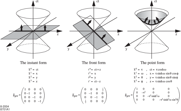
Figure 1: The three forms of Hamiltonian dynamics Dirac ; BPPreport . In the front form (middle), initial conditions are defined on a light-like surface, and the system is the propagated in light-cone time $x^{+}$ by the light-cone Hamiltonian $\widehat{P}^{-}$.

Another advantage of the light-front formulation of thermal field theory is that the charge is defined as the integral over the $+$-component of the current density, $Q=\int d^{3}rj^{+}(\vec{r})$. This allows one to establish a clear connection between densities in thermal field theory and the boost-invariant parton distributions measured in hard scattering experiments fact . No such relation exists in the instant form, where charges are integrals over $0$-components of current densities. Also, parton distributions defined in equal-time quantization are not boost invariant, since the generator of Lorentz transformations in $r_{3}$ direction contains interaction terms. As a consequence, in this formalism one might regard low-$x$ gluon saturation as a phase transition BNL or a critical phenomenon Pirner in the sense of statistical mechanics. One can even generalize the concept of a parton distribution to finite temperature, which is relevant for jet quenching in heavy ion collisions Ivan as well as for parton recombination Rainer .

We also point out that fermions behave completely differently on the light-front, where they are described terms of just 2-component spinors. It turns out that the fermion propagator has only one derivative in the numerator, leading to only one pair of doublers on the lattice. In addition, the doubler problem is entirely avoided in Discretized Light-Cone Quantization (DLCQ) DLCQ . This technique is also applicable at finite density and will hopefully allow one to study baryon-rich QCD matter in large scale numerical calculations. Despite recent progress Fodor , conventional lattice QCD is still notoriously complicated at finite baryon chemical potential.

This paper is organized as follows. In the next section, we construct the most general form of the statistical operator allowed by the Poincaré algebra. Our results are in agreement with earlier findings diplom ; Das ; Weldon . We argue that the simplicity of the vacuum does not lead to difficulties when describing phase transitions. In Section III, we define gauge-invariant Green’s functions for fermions at finite temperature and relate them to generalized parton distributions in Section IV. In the summary, we give an outlook on further applications and challenges for this approach.

II The statistical operator at finite temperature and density

The form of the statistical operator ${\widehat{w}}$ at finite temperature and density can be obtained from very general considerations. Our result below for ${\widehat{w}}$, Eq. (5), is compatible with the findings of Alves ; Weldon , i.e. ${\widehat{w}}$ is always the exponential of the equal time energy $\widehat{P}^{0}$ in the local rest frame of the system. Here, we shall give a more physical derivation of that result, following Ref. Landau5 .

In the instant form, the equal time Liouville theorem (${\imath}\partial^{0}{\widehat{w}}_{ET}=[\widehat{P}^{0},{\widehat{w}}_{ET}]$) requires that in equilibrium, ${\widehat{w}}_{ET}$ is a function of only those Poincaré generators which commute with the equal time Hamiltonian $\widehat{P}^{0}$. In addition, since systems far apart from each other must be uncorrelated, the density operator of the combined system has to factorize into the density operators of the subsystems. This requirement is similar to the cluster decomposition principle that has been studied in the context of the deuteron wavefunction on the light-cone in Ref. cluster . Consequently, in equilibrium $\ln({\widehat{w}}_{ET})$ must be a linear combination of the additive constants of motion, namely the four components of the momentum $\widehat{P}^{\mu}$ and the angular momentum three-vector $\vec{J}$. Hence, $\ln({\widehat{w}}_{ET})=\alpha-\beta(u_{\nu}\widehat{P}^{\nu}-\vec{\omega}\cdot\vec{J}-\sum_{l}\mu_{l}\widehat{Q}_{l})$, where $\alpha$ is a normalization constant. The notation is chosen in anticipation of the physical meaning of the various coefficients: $\beta$ is the inverse temperature and $u_{\nu}$ is the four velocity of the system, cf. Ref. Alves . In addition, $\vec{\omega}$ is the angular velocity at which the body rotates. Additional conserved charges $\widehat{Q}_{l}$ are included along with their chemical potentials $\mu_{l}$. We stress that the “charges”, i.e. the mean values of the operators $\widehat{P}_{\nu},\vec{J},\widehat{Q}_{l}$, are given and that the “chemical potentials” ($u_{\nu},\vec{\omega},\mu_{l}$) need to be determined from the conservation laws. In quantum mechanics, of course, one can simultaneously specify only charges which commute with each other, i.e. only one component of $\vec{J}$ (namely for rotations around the axis with the largest moment of inertia.) For the same reason, one cannot specify all four $P_{\nu}$ for systems with nonzero angular momentum.

What changes, when we switch to the light front? First of all, the equal time Liouville theorem has to be replaced by its light front analog. Writing the light front density operator as

$${\widehat{w}}=\sum_{ij}c_{ij}\left|\phi_{i}\rangle\langle\phi_{j}\right|,$$ (1)

the (light cone) time ($x^{+}$) evolution of the multi particle state $\left|\phi_{i}\rangle\right.$ is generated by the second quantized Hamiltonian $\widehat{P}^{-}$,

$${\imath}\partial^{-}\left|\phi_{i}\rangle\right.=\widehat{P}^{-}\left|\phi_{i}\rangle\right..$$ (2)

From this, the light front version of the Liouville theorem immediately follows:

$${\imath}\partial^{-}{\widehat{w}}=\left[\widehat{P}^{-},{\widehat{w}}\right].$$ (3)

Equilibrium (on the light front) is reached, when the commutator on the right hand side (rhs) of Eq. (3) vanishes. The six Poincaré generators which commute with $\widehat{P}^{-}$ are the other three momentum components and three of the six independent elements of the antisymmetric boost-angular momentum tensor

$$\widehat{M}^{\kappa\nu}=\left(\begin{array}[]{cccc}0&\widehat{K}_{1}+\widehat{J}_{2}&\widehat{K}_{2}-\widehat{J}_{1}&-2\widehat{K}_{3}\\ -\widehat{K}_{1}-\widehat{J}_{2}&0&\widehat{J}_{3}&-\widehat{K}_{1}+\widehat{J}_{2}\\ -\widehat{K}_{2}+\widehat{J}_{1}&-\widehat{J}_{3}&0&-\widehat{K}_{2}-\widehat{J}_{1}\\ 2\widehat{K}_{3}&\widehat{K}_{1}-\widehat{J}_{2}&\widehat{K}_{2}+\widehat{J}_{1}&0\end{array}\right)$$ (4)

($\mu,\nu\in\{+,1,2,-\}$). Namely the rotations ($\widehat{M}^{1,2}=\widehat{J}_{3}$) around the longitudinal direction and the two dynamic operators $\widehat{M}^{\perp-}=(\widehat{M}^{1-},\widehat{M}^{2-})$, where $\widehat{M}^{1-}=-\widehat{K}_{1}+\widehat{J}_{2}$, $\widehat{M}^{2-}=-\widehat{K}_{2}-\widehat{J}_{1}$. The $\widehat{K}_{j}$ are boost generators in $j$ direction. Since two of the operators $\widehat{M}^{\perp-}$ have zero eigenvalues when acting on all physical states, the light front density operator has the general form

$$\ln({\widehat{w}})=\alpha-\beta\left(u_{\nu}\widehat{P}^{\nu}-\omega\widehat{J}_{3}-\sum_{l}\mu_{l}\widehat{Q}_{l}\right).$$ (5)

Thus we have obtained the same Jüttner type distribution as in the instant form. The identification of $u_{\nu}$ with the four-velocity of the system relative to the observer can be derived by calculating the commutators of $\ln({\widehat{w}})$ with the boost generators by means of the Poincaré algebra. Since $u_{\nu}u^{\nu}=1$, only four of the five parameters $\beta=1/T$ and $u^{\nu}$ are independent.

We remark that $T$ is the same as the instant-form temperature, but the chemical potential has a different meaning. On the light-front, densities are given by $+$-components of currents, and not by $0$-components. This is essential for the proper generalization of parton distributions to finite temperature, since the latter are also defined as $+$-components fact .

Note that one can include rotations in the light front formalism, but one has to make sure that the longitudinal axis has the largest inertial moment. Of course, one cannot specify $\vec{P}_{\perp}$ and $J_{3}$ simultaneously. We shall not study systems with finite angular momentum in what follows.

We choose $\alpha=0$ as normalization so that the partition function is given by ${\cal Z}={\rm Tr}{\widehat{w}}$. Since $\cal Z$ is a Lorentz scalar, all thermodynamic potentials and the entropy transform as scalars, e.g. the Lorentz invariant generalization of the grand-canonical potential (or of the free energy in the case of $\mu=0$) is

$$\Omega=-T\ln{\cal Z}(V,T,\mu),$$ (6)

and the entropy is defined by

$$S=-\left(\frac{\partial\Omega}{\partial T}\right)_{\mu,V}=-\frac{1}{\cal Z}{\rm Tr}({\widehat{w}}\ln{\widehat{w}}).$$ (7)

The role of the total energy of the system is now played by the expectation value of $u_{\nu}\widehat{P}^{\nu}$,

$$U=\langle u_{\nu}\widehat{P}^{\nu}\rangle=\frac{u_{\nu}}{\cal Z}{\rm Tr}({\widehat{w}}\widehat{P}^{\nu}).$$ (8)

As usual, $\Omega=U-TS-\mu Q$. All known relations between thermodynamic potentials remain valid.

Even though one can formulate light-front statistical mechanics in an arbitrary frame, it is convenient to choose the reference frame in which the system as a whole is at rest, so that $\ln({\widehat{w}})=-\beta\widehat{P}^{0}$. Since the three forms of Hamiltonian Dynamics are not related by Lorentz transformations, there is no frame in which $\widehat{P}^{+}=0$. Therefore, ${\widehat{w}}\neq\exp(-\beta_{LC}\widehat{P}^{-})$ (cf. Ref. Alves ; Weldon ).

The quantities $\beta$, $u_{\nu}$, $\omega$ and $\mu_{l}$, have the meaning of Lagrange multipliers that hold the mean values of the constants of motion fixed, while entropy is maximized. In an ideal gas for example, the maximum entropy is attained for occupation numbers given by Fermi-Dirac and Bose-Einstein statistics Alves ; Beyer ,

$$n(u_{\nu}p^{\nu})=\frac{g}{{\rm e}^{\beta(u_{\nu}p^{\nu}-\mu)}\pm 1}-\frac{g}{{\rm e}^{\beta(u_{\nu}p^{\nu}+\mu)}\pm 1},$$ (9)

assuming that particles carry charge $+1$ and antiparticles charge $-1$. (Note that $u_{\nu}p^{\nu}\geq 0$.) Here, $p^{\nu}$ is the 4-momentum of a single particle and the degeneracy factor for different spin states is denoted by $g$. The Lagrange multipliers define the equilibrium conditions for two systems. In complete equilibrium with each other, both systems must have the same values of temperature, $u_{\nu}$, $\omega$ and $\mu_{l}$, i.e. no internal motion of macroscopic parts of the system is possible in equilibrium (at least in the absence of vortex lines Landau5 .) In particular, the system cannot perform a relative motion with respect to an external heat bath. It is important in this respect that the values of these Lagrange multipliers do not depend on the total size of the system. Thus, even though one can rewrite the statistical operator in terms of light-front momentum fractions $x_{l}$ and the total invariant mass squared ($M^{2}$) as (let $\vec{P}_{\perp}=\vec{0}_{\perp}$ and all $Q_{l}=0$)

$${\widehat{w}}=\exp(-\gamma_{x}\sum_{l}x_{l}-\gamma_{M^{2}}M^{2})$$ (10)

the quantities $\gamma_{x}=u^{-}P^{+}/(2T)$ and $\gamma_{M^{2}}=u^{+}/(2TP^{+})$ depend on the overall size of the system and are therefore unsuitable to define equilibrium conditions. For that reason, some care is required when talking about phase diagrams in the $x$-$M^{2}$ plane, which is often done in the context of the Color Glass Condensate BNL .

As usual, the (grand) canonical ensemble allows for fluctuations of the total momentum and of the total charge. Since we have constructed ${\widehat{w}}$ such that it depends only on extensive quantities, the relative magnitude of these fluctuations becomes irrelevant for large systems such as a neutron star, i.e.

$$\frac{\sqrt{\left(\Delta P^{\nu}\right)^{2}}}{P^{\nu}}\propto\frac{1}{\sqrt{N}},$$ (11)

for each $\nu$. Here $N$ is the number of quanta in the system. For a large enough system one can therefore use the canonical or the grand canonical ensembles, which are much more convenient for calculations than the microcanonical ensemble, even if the values of $P^{\nu}$, $J_{3}$ and $Q_{l}$ are strictly conserved. For a large nucleus, $N\mathrel{\hbox to0.0pt{\lower 4.0pt\hbox{\hskip 1.0pt$\sim$}\hss}\raise 1.0pt\hbox{$>$}}10^{3}$. This means a statistical approach is still justified. For a single hadron however, the microcanonical ensemble with strict conservation of the constants of motion is more appropriate liu .

The simplicity of the light-front vacuum, usually considered an advantage, seems to bear problems as far as phase transitions are concerned. Clearly, thermal field theory on the light-front would be rendered useless if it turned out that the zero-mode problem SSB ; kazu would have to be solved before any statements about phase transitions could be made. However, the fact that the statistical weight of a configuration is maximized for minimal equal-time energy rather than for minimal light-front energy has important consequences for the formation of condensates at low temperatures. The ground state, i.e. the state the system is in at $T=0$, is in general different from the light-front vacuum. (Indeed, for massive particles $P^{-}=0$ corresponds to infinite $P^{0}$.)

Alves, Das and Perez Alves obtained the self-energy to one-loop order in $\phi^{4}$ theory (${\cal L}=\partial_{\nu}\phi^{*}\partial^{\nu}\phi-m^{2}\phi^{*}\phi-\lambda(\phi^{*}\phi)^{2}$). Replacing $-m^{2}$ with $c^{2}>0$, one immediately obtains spontaneous symmetry breaking from their results, including a massless Goldstone boson. No problem arises from $1/k^{+}$-poles. As usual, one of the fields in this model develops a non-vanishing expectation value and is shifted correspondingly. One of the redefined fields, the $\sigma$, acquires a finite mass. The other field is massless and will be referred to as $\pi$ here. In the high temperature limit, the masses obtained from the one-loop calculation of Ref. Alves are given by the simple expressions

$$m_{\sigma}^{2} = \left\{\begin{array}[]{lr}2c^{2}(1-T^{2}/T_{c}^{2}),&\quad T\leq T_{c}\\ \frac{1}{3}\lambda(T^{2}-T_{c}^{2}),&\quad T\geq T_{c}\end{array}\right.$$ (14)

$$m_{\pi}^{2} = \left\{\begin{array}[]{lr}0,&\quad T\leq T_{c}\\ \frac{1}{3}\lambda(T^{2}-T_{c}^{2}),&\quad T\geq T_{c}\end{array}\right.,$$ (17)

with $T_{c}=3c^{2}/\lambda$. These are the standard results Kapusta . The broken phase has one massive sigma and one massless pion. There is a second order phase-transition at $T=T_{c}$, where all masses vanish. In the symmetric phase, all fields have the same mass.

In addition, the authors of Ref. Beyer reproduced the chiral phase transition in the Nambu–Jona-Lasinio Model on the light-front.

The possibility of spontaneous symmetry breaking without zero-modes has previously been suggested in Ref. Thorn for $\phi^{4}$(1+1), but these authors did not study the finite temperature case. Nevertheless, the picture arising in our work is similar to that of Ref. Thorn , where $P^{-}$ is minimized, keeping the total $P^{+}$ fixed by introducing a Lagrange multiplier. In our approach, on the other hand, the equilibrium configuration is found by maximizing the entropy for fixed mean values of all four momentum components.

We conclude that this approach is poised for the study of phase transitions in more complicated field theories, such as QCD.

III Fermion Green’s function in a medium

Until now one could get the impression that thermodynamics and statistical physics on the light front is identical to the usual instant form approach, except for a trivial change of variables. That this is not the case becomes most clear, when one studies fermions on the light-front.

In light-front field theory, the Dirac equations can be written as a set of two coupled equations for 2-component spinors, see appendix A. Only one of these equations contains a time derivative, the other one is a constraint. As a consequence, the entire theory can be formulated in terms of 2-component spinors, very much like a non-relativistic theory. It is however important to note, that the 2-component theory does not follow from a local, scalar Lagrangian. The theory is non-local, because the action can propagate “instantaneously” along the light-line, where the quantization surface touches the light-cone (see Fig. 1). This often leads to difficulties known as the zero-mode problem. We believe that these difficulties can be overcome by introducing time-ordered, retarded and advanced Green’s functions directly in the Hamiltonian formulation. This is done in Ref. Landau9 for the non-relativistic case, in which non-local operators are common, since particles interact through potentials. Nevertheless, in a diagrammatic expansion of these Green’s functions, all 4 momentum components are conserved at each vertex. The Green’s function is the fundamental object of this approach.

To define the various Green’s functions of a fermion in a medium, we first introduce Heisenberg field operators for the dynamical spinor components ($\alpha\in\{1,2\}$),

$$\widehat{\psi}_{\alpha}(r) = {\rm e}^{\imath\widehat{P}^{-}r^{+}/2}\widehat{\Psi}_{\alpha}(\underline{r}){\rm e}^{-\imath\widehat{P}^{-}r^{+}/2},$$ (18)

$$\widehat{\psi}_{\alpha}^{\dagger}(r) = {\rm e}^{\imath\widehat{P}^{-}r^{+}/2}\widehat{\Psi}_{\alpha}^{\dagger}(\underline{r}){\rm e}^{-\imath\widehat{P}^{-}r^{+}/2}.$$ (19)

At equal $r^{+}$, these Heisenberg operators fulfill the same anticommutation relations, Eq. (75), as the Schrödinger operators.

The time-ordered Green’s functions of a fermion in a medium is defined in terms of the dynamical fields only Alves ; Prem ,

$$\imath G_{\alpha,\beta}(r_{1},r_{2}) = \langle T_{+}\widehat{\psi}_{\alpha}(r_{1})\widehat{\psi}_{\beta}^{\dagger}(r_{2})\rangle$$ (20)

$$= \langle\widehat{\psi}_{\alpha}(r_{1})\widehat{\psi}_{\beta}^{\dagger}(r_{2})\rangle\Theta(r_{1}^{+}-r_{2}^{+})-\langle\widehat{\psi}_{\beta}^{\dagger}(r_{2})\widehat{\psi}_{\alpha}(r_{1})\rangle\Theta(r_{2}^{+}-r_{1}^{+}),$$ (21)

where the average,

$$\langle\dots\rangle=\frac{{\rm Tr}(\dots{\widehat{w}})}{{\cal Z}},$$ (22)

is to be taken with the appropriate ensemble, i.e. canonical or grand canonical for large systems or microcanonical for hadrons. This definition of the Green’s function includes the case of zero temperature. Therefore, the conventional light-front quantization at temperature $T=0$ can be formulated in terms of $G_{\alpha,\beta}$ as well.

We stress that the Green’s function in light-front quantization is not a Lorentz scalar, in contrast to equal-time quantization. In addition, for isotropic and homogeneous systems, the $G_{\alpha,\beta}$ have the general form ($r=r_{1}-r_{2}$)

$$G_{\alpha,\beta}(r_{1},r_{2})=\delta_{\alpha,\beta}G(r),$$ (23)

which is completely different from the fermion propagator in equal-time field theory. While $G$ is an even function of $\vec{r}_{\perp}$, i.e. $G(r^{+},r^{-},\vec{r}_{\perp})=G(r^{+},r^{-},-\vec{r}_{\perp})$, it can be seen from the definition Eq. (20) that $G$ is not an even function of $r^{+}$. Neither is $G$ an even function of $r^{-}$, because the field operators, Eqs. (72,73), are not defined for negative $k^{+}$, so that the Fourier transform $\widetilde{G}_{\alpha,\beta}(k)$ has a cut along the negative $k^{+}$ axis. This cut is needed to obtain separate information about fermion and antifermion distributions from the Green’s function. The analytic structure of the light-front Green’s function is therefore rather complicated.

The Green’s function in momentum space is given by

$$\widetilde{G}_{\alpha,\beta}(k)=\int d^{4}r{\rm e}^{\imath kr}G_{\alpha,\beta}(r),$$ (24)

and the inverse of this transformation is

$$G_{\alpha,\beta}(r)=\int\frac{d^{4}k}{(2\pi)^{4}}\Theta(k^{+})\left({\rm e}^{-\imath k^{+}r^{-}/2}+{\rm e}^{+\imath k^{+}r^{-}/2}\right){\rm e}^{-\imath k^{-}r^{+}/2}{\rm e}^{+\imath\vec{k}_{\perp}\vec{r}_{\perp}}\widetilde{G}_{\alpha,\beta}(k).$$ (25)

In a gauge theory, it is also necessary to include a (path ordered) gauge connector along the light-cone by redefining the fermion fields,

$$\widehat{\psi}_{\alpha}(r_{1}) \to \widehat{\psi}_{\alpha}(r_{1})P\exp\{\frac{ig}{2}\int_{-\infty}^{r_{1}^{-}}dr^{-}A^{+}(r_{1}^{+},r^{-},\vec{r}_{1,\perp})\},$$ (26)

$$\widehat{\psi}_{\beta}^{\dagger}(r_{2}) \to \widehat{\psi}_{\beta}^{\dagger}(r_{2})\left[P\exp\{\frac{ig}{2}\int_{-\infty}^{r_{2}^{-}}dr^{-}A^{+}(r_{2}^{+},r^{-},\vec{r}_{2,\perp})\}\right]^{\dagger}.$$ (27)

The path-ordering symbol $P$ arranges the gauge fields $A^{+}(r)$ in order of ascending $r^{-}$, i.e. with the largest $r^{-}$ to the left. This redefinition does not affect the anti-commutation relations Eq. (75) of the fermion fields. Inclusion of the gauge connector makes the Green’s function gauge invariant in the limit $r_{1}^{+}-r_{2}^{+}\to\pm 0$, $\vec{r}_{1,\perp}\to\vec{r}_{2,\perp}$. The time evolution of $G_{\alpha,\beta}$ is given by

$$2\imath\frac{\partial}{\partial r_{1}^{+}}G_{\alpha,\beta}(r_{1},r_{2})-\langle T_{+}\left[\widehat{\psi}_{\alpha}(r_{1}),\widehat{P}^{-}\right]\widehat{\psi}_{\beta}^{\dagger}(r_{2})\rangle=\delta_{\alpha,\beta}\delta^{(4)}(r_{1}-r_{2}).$$ (28)

Note that a gauge invariant Hamiltonian $\widehat{P}^{-}$ alone is not sufficient to make $G_{\alpha,\beta}$ gauge invariant. One also has to include the path-ordered exponentials as in Eqs. (26,27).

A possible subtlety arises in light-cone gauge, $A^{+}=0$. Even though the path-ordered exponentials reduce to unity, they may still influence the time evolution of $G_{\alpha,\beta}$ because their commutator with $\widehat{P}^{-}$ will in general not vanish, i.e.

$$\left[\widehat{\psi}_{\alpha}(r_{1})|_{A^{+}=0},\widehat{P}^{-}_{A^{+}=0}\right]\neq\left[\widehat{\psi}_{\alpha}(r_{1}),\widehat{P}^{-}\right]_{A^{+}=0}.$$ (29)

In ordinary light-front quantization at $T=0$, the gauge link is associated with the single-spin asymmetry SSA . Its role at finite temperature is yet to be explored.

In addition, the retarded ($R$) and advanced ($A$) Green’s functions are defined by the anticommutators

$$\imath G^{R}_{\alpha,\beta}(r_{1},r_{2}) = \langle\left\{\widehat{\psi}_{\alpha}(r_{1}),\widehat{\psi}_{\beta}^{\dagger}(r_{2})\right\}\rangle\Theta(r_{1}^{+}-r_{2}^{+}),$$ (30)

$$\imath G^{A}_{\alpha,\beta}(r_{1},r_{2}) = -\langle\left\{\widehat{\psi}_{\alpha}(r_{1}),\widehat{\psi}_{\beta}^{\dagger}(r_{2})\right\}\rangle\Theta(r_{2}^{+}-r_{1}^{+}).$$ (31)

These Green’s functions are needed in finite temperature perturbation theory and obey Eq. (28) as well. The time-ordered Green’s function $G_{\alpha,\beta}$ is related to $G_{\alpha,\beta}^{A}$ and $G_{\alpha,\beta}^{R}$ by Landau9 ,

$$\widetilde{G}_{\alpha,\beta}(k)=\frac{1}{2}\left(\widetilde{G}^{R}_{\alpha,\beta}(k)+\widetilde{G}^{A}_{\alpha,\beta}(k)\right)+\frac{1}{2}{\rm tanh}\left(\frac{uk}{2T}\right)\left(\widetilde{G}^{R}_{\alpha,\beta}(k)-\widetilde{G}^{A}_{\alpha,\beta}(k)\right).$$ (32)

In order to obtain this formula, it is important that the Green’s function can be interpreted in terms of transition amplitudes. This is possible, even in a gauge theory, because the gauge link between the fermion fields at $r_{1}$ and $r_{2}$ can be absorbed into a redefinition of the field operators, see Eq. (26,27). Note that at $T=0$, $\widetilde{G}_{\alpha,\beta}(k)=\widetilde{G}^{R}_{\alpha,\beta}(k)$ for positive energy solutions and $\widetilde{G}_{\alpha,\beta}(k)=\widetilde{G}^{A}_{\alpha,\beta}(k)$ for negative energy solutions.

In the free theory, all Green’s functions fulfill the integro-differential equation,

$$\left[\imath\partial^{-}_{1}-\frac{-\partial_{1\perp}^{2}+m^{2}}{\imath\partial^{+}_{1}}\right]G^{(0),(X)}_{\alpha,\beta}(r_{1},r_{2})=\delta_{\alpha,\beta}\delta^{(4)}(r_{1}-r_{2}),$$ (33)

with boundary conditions appropriate to their physical meaning. The Green’s functions of a fermion in an ideal gas of temperature $T=1/\beta$ were presented first in Ref. Alves . In momentum space, adjusted to our notation, they read

$$\widetilde{G}^{(0)R}_{\alpha,\beta}(k) = \delta_{\alpha,\beta}\frac{k^{+}}{k^{2}-m^{2}+\imath\epsilon{\rm sgn}(uk)},$$ (34)

$$\widetilde{G}^{(0)A}_{\alpha,\beta}(k) = \delta_{\alpha,\beta}\frac{k^{+}}{k^{2}-m^{2}-\imath\epsilon{\rm sgn}(uk)},$$ (35)

$$\widetilde{G}^{(0)}_{\alpha,\beta}(k) = \delta_{\alpha,\beta}\left({\rm P}\frac{k^{+}}{k^{2}-m^{2}}-\imath{\rm sgn}(uk)\pi{\rm tanh}\left(\frac{uk}{2T}\right)k^{+}\delta(k^{2}-m^{2})\right),$$ (36)

where ${\rm P}$ refers to principle value prescription. In the limit $T\to 0$, the light-front Feynman propagator for fermions turns out to be

$$S_{F}(k)=\delta_{\alpha,\beta}\frac{k^{+}}{k^{2}-m^{2}+\imath\epsilon},$$ (37)

which agrees with the result obtained earlier in Ref. Prem with a different technique.

The pole prescriptions $\pm\imath\epsilon{\rm sgn}(uk)$ for the retarded and advanced Green’s functions are another manifestation of the special meaning of the equal-time energy. These prescriptions ensure that $G^{(0)R}_{\alpha,\beta}(r)$ vanishes outside the forward lightcone, while $G^{(0)A}_{\alpha,\beta}(r)$ is non-vanishing only inside the backward lightcone. That this is indeed the case can be seen by comparing $\widetilde{G}^{(0)R}_{\alpha,\beta}(k)$ and $\widetilde{G}^{(0)A}_{\alpha,\beta}(k)$ to the well-known propagators of a scalar particle Peskin , which differ only by the overall factor $\delta_{\alpha,\beta}k^{+}$ from the fermion Green’s functions in light-front quantization.

Most importantly, knowledge of the correct pole prescription eliminates ambiguities in the definition of the non-local operator $1/k^{+}$, which appears e.g. in the free light-cone Hamiltonian, Eq. (80). However, the correct prescription for the $1/k^{+}$-pole depends on the type of Green’s function and on the value of the other momentum components. The easiest way to overcome these complications is to construct a perturbative expansion of $G$ from Eq. (28). The 4-dimensional $\delta$-function on the right hand side leads to 4-dimensional integrals in momentum space, of the kind in Eq. (25). This type of perturbation theory is by no means identical to the usual Feynman perturbation theory in equal-time quantization, as can be seen immediately from the free propagators. Nevertheless, observable quantities must be the same in both formulations, at least within experimental error bars. First applications Prem at $T=0$ indicate that this is the case.

It is possible to introduce the chemical potential in this formalism in a covariant way. (See also Ref. Beyer .) The effective Hamiltonian in thermal field theory on the light-front is

$$\widehat{\cal H}=u_{\nu}\widehat{P}^{\nu}-\mu\widehat{Q}.$$ (38)

This operator propagates the system in proper time $\tau$. Since in equilibrium $u_{\nu}$ is independent of space time, $r^{\nu}=u^{\nu}\tau$. The presence of a chemical potential then modifies the generators of space-time translations as if $\mu u^{\nu}$ were a gauge field. The modified translation generators read

$${\widehat{\cal P}}^{\nu}=\widehat{P}^{\nu}-\mu\widehat{Q}u^{\nu}.$$ (39)

They propagate the system along trajectories of constant charge and take into account that the medium moves as a whole as the “test particle” represented by the Green’s function propagates from $r_{2}$ to $r_{1}$. The definition of the Heisenberg operators has to be changed accordingly, i.e. one needs to replace $\widehat{P}^{-}$ by ${\widehat{\cal P}}^{-}$ in Eqs. (18,19).

Another remarkable property of the light-front Green’s functions is, that if the theory is discretized on a lattice in $\underline{r}$-space, the factor $k^{+}$ in the numerator leads to only one pair of fermion doublers. Naturally, this simplification comes at a price. In QCD for example, the light-front Hamiltonian contains non-local terms $\propto 1/k^{+}$ and $\propto 1/(k^{+})^{2}$ BPPreport . In order to calculate the Green’s function on a light-front lattice, one needs to find field configurations with maximum statistical weight, as determined from ${\widehat{w}}$. This can in principle be done with the Metropolis algorithm Metro . Unfortunately, each configuration update requires the evaluation of two integrals (because of the $\propto 1/(k^{+})^{2}$-terms) over the light-cone (for every lattice site.) It is at present not clear, if this disadvantage outweighs the absence of most doubler states. However, we argue that a light-front lattice is advantageous at large chemical potential, where Monte-Carlo techniques usually cannot be applied because of the sign problem. There is no fermion determinant in the Hamiltonian approach developed here, and also the chemical potential enters in a different way, see Eq. (39). A further investigation of light-front lattice techniques seems therefore interesting to us. Results from transverse lattice calculations at finite temperature have been published recently as well SD .

In Discretized Light-Cone Quantization DLCQ DLCQ , the alternative non-perturbative technique in quantum field theory, it is already known that no fermion doubling problem occurs. Furthermore, it is possible to do calculations for a fixed value of the total charge without any sign problem. The output of DLCQ is the full spectrum of the theory, i.e. all masses of the energy eigenstates and their wavefunctions. This is of course much more information than is needed to calculate bulk thermodynamic properties. Nevertheless, from the DLCQ solution of a field theory, one can directly obtain the partition function. This was actually done in Ref. alex for QED(1+1).

Once the Green’s function is known numerically from any method, one can calculate all thermodynamic properties of the system by integrating the relation

$$\left(\frac{\partial\Omega}{\partial\mu}\right)_{V,T}=-Q.$$ (40)

In fact, it is sufficient to know $G(r)$ for all $\mu$ and $T$ in the limit $r\to 0^{-}$ to calculate the grand-canonical potential $\Omega$. From this, the equation of state and hence the phase structure of the theory immediately follow. The relation of $G_{\alpha,\beta}$ to the total charge $Q$ will be explained in more detail in the next section.

IV The light-front density matrix and generalized parton distributions

The physical meaning of the time-ordered Green’s function $G_{\alpha,\beta}$ is eludicated further by comparing its definition, Eq. (20), with the charge operator in Eq. (76). One observes that the net charge distribution in coordinate space is given by

$$Q(\underline{r})=-\imath G_{\alpha,\alpha}(r^{+}\to 0^{-},\underline{r}|r^{+},\underline{r}).$$ (41)

Summation over $\alpha$ is understood. The notation $r^{+}\to 0^{-}$ means that the limit $r^{+}\to 0$ is to be taken from below. The value of the chemical potential $\mu$ as a function of temperature $T$ and total charge $Q$ is then determined by the equation

$$Q=-\imath\int d^{3}rG_{\alpha,\alpha}(r^{+}\to 0^{-},\underline{r}|r^{+},\underline{r}).$$ (42)

Of course, the density $Q(\underline{r})$ is constant, if $G_{\alpha,\beta}(r_{1},r_{2})=G_{\alpha,\beta}(r_{1}-r_{2})$.

In this section, we introduce the light-front density matrix, which is related to the light-cone wavefunctions of Ref. BL in the same way as the one-particle density matrix is related to the wavefunction of a system in non-relativistic quantum mechanics. If the system is a hadron or a nucleus, the diagonal elements of the light-front density matrix are the parton distributions measured in hard scattering experiments, while the off-diagonal matrix elements turn out to be generalized parton distributions (GPDs) gpdf1 ; Ji ; Rady . This illustrates that the quark and gluon distributions in a hadron are not classical densities, but quantum mechanical quantities.

Finding all light-front wavefunctions for a hadron is equivalent to solving the QCD bound state equation

$$\widehat{P}^{-}|h\rangle=\frac{\vec{P}_{\perp}+M_{h}^{2}}{P^{+}}|h\rangle.$$ (43)

This has been accomplished for QCD in $1+1$ dimensions Kent , but is a formidable task in any $3+1$ dimensional field theory. On the other hand, if the system is large enough, such as a heavy nucleus, a heavy ion collision, or a neutron star, one can hope that a statistical approach may be viable. In fact, for a system with a very large number of partons, say $>10^{3}$, the density-matrix is probably more useful a concept than the light-front wavefunctions.

Knowledge of the density matrix enables one to calculate the expectation value of any single-particle operator, i.e. any operator that can be written as

$$\widehat{F}_{\alpha,\beta}(r^{+})=\int d^{3}r\widehat{\psi}^{\dagger}_{\alpha}(r)\widehat{f}_{\beta,\gamma}\widehat{\psi}_{\gamma}(r)$$ (44)

in second quantization. The density matrix provides only an incomplete description of the system, but is sufficient for many applications of statistical physics.

A relation similar to Eq. (41) exists in condensed matter physics Landau9 , but in light-front field theory the situation is more complicated due to the presence of anti-particles. For example, one is tempted to interpret

$$Q_{\alpha,\beta}(\underline{r}_{1},\underline{r}_{2})=-\imath G_{\alpha,\beta}(r_{2}^{+}\to 0^{-},\underline{r}_{1}|r_{2}^{+},\underline{r}_{2})=\langle\widehat{\psi}_{\beta}^{\dagger}(r_{2})\widehat{\psi}_{\alpha}(r_{1})\rangle\big{|}_{r_{1}^{+}=r_{2}^{+}}$$ (45)

as the density matrix of the net charge distribution in the system, in analogy to non-relativistic Fermi systems. However, since the total charge $Q$ can have either sign, one cannot normalize $Q_{\alpha,\beta}(\underline{r}_{1},\underline{r}_{2})$ simply by dividing it by $Q$. Therefore, knowledge of $Q_{\alpha,\beta}(\underline{r}_{1},\underline{r}_{2})$ does not immediately enable one to calculate the expectation value of single-particle operators. One first needs to find separate density matrices for fermions and antifermions, $q_{\alpha,\beta}(\underline{r}_{1},\underline{r}_{2})$ and $\overline{q}_{\alpha,\beta}(\underline{r}_{1},\underline{r}_{2})$. Then,

$$\langle\widehat{F}_{\alpha,\beta}(r^{+})\rangle=\frac{\int d^{3}r_{1}d^{3}r_{2}\widehat{f}^{(1)}_{\beta,\alpha}\left[q_{\alpha,\beta}(\underline{r}_{1},\underline{r}_{2})+\overline{q}_{\alpha,\beta}(\underline{r}_{1},\underline{r}_{2})\right]\delta^{(3)}(\underline{r}_{1}-\underline{r}_{2})}{\int d^{3}r\left[q_{\alpha,\alpha}(\underline{r},\underline{r})+\overline{q}_{\alpha,\alpha}(\underline{r},\underline{r})\right]},$$ (46)

with $f^{(1)}_{\beta,\alpha}$ acting on $\underline{r}_{1}$.

In the 2-component theory, the separation of fermion and antifermion distributions requires the evaluation of a Fourier-integral of the Green’s function. Since $G_{\alpha,\beta}(r_{1},r_{2})$ often depends only on the difference $r=r_{1}-r_{2}$, it is natural to introduce the variables

$$R = \frac{r_{1}+r_{2}}{2},$$ (47)

$$r = r_{1}-r_{2}.$$ (48)

The first step in finding an expression for the quark density matrix is to write down the operator structure of $Q_{\alpha,\beta}$,

$$Q_{\alpha,\beta}(\underline{r}_{1},\underline{r}_{2}) = \langle\widehat{\psi}_{\beta}^{\dagger}(R-\frac{r}{2})\widehat{\psi}_{\alpha}(R+\frac{r}{2})\rangle\big{|}_{r_{1}^{+}=r_{2}^{+}}$$

$$= \left<\sum_{\lambda_{1},\lambda_{2}}\int\frac{d^{3}k_{1}}{2(2\pi)^{3}\sqrt{k_{1}^{+}}}\Theta(k_{1}^{+})\int\frac{d^{3}k_{2}}{2(2\pi)^{3}\sqrt{k_{2}^{+}}}\Theta(k_{2}^{+})\right.$$

$$\left\{\widehat{b}^{\dagger}(\underline{k}_{2},\lambda_{2})\widehat{b}(\underline{k}_{1},\lambda_{1})\chi^{\dagger}_{\beta}(\lambda_{2})\chi_{\alpha}(\lambda_{1}){\rm e}^{+\imath\underline{k}_{2}\cdot\left(\underline{R}-\frac{\underline{r}}{2}\right)-\imath\underline{k}_{1}\cdot\left(\underline{R}+\frac{\underline{r}}{2}\right)}\right.$$

$$+ \widehat{d}(\underline{k}_{2},\lambda_{2})\widehat{d}^{\dagger}(\underline{k}_{1},\lambda_{1})\chi^{\dagger}_{\beta}(-\lambda_{2})\chi_{\alpha}(-\lambda_{1}){\rm e}^{-\imath\underline{k}_{2}\cdot\left(\underline{R}-\frac{\underline{r}}{2}\right)+\imath\underline{k}_{1}\cdot\left(\underline{R}+\frac{\underline{r}}{2}\right)}$$

$$+ \widehat{b}^{\dagger}(\underline{k}_{2},\lambda_{2})\widehat{d}^{\dagger}(\underline{k}_{1},\lambda_{1})\chi^{\dagger}_{\beta}(\lambda_{2})\chi_{\alpha}(-\lambda_{1}){\rm e}^{+\imath\underline{k}_{2}\cdot\left(\underline{R}-\frac{\underline{r}}{2}\right)+\imath\underline{k}_{1}\cdot\left(\underline{R}+\frac{\underline{r}}{2}\right)}$$

$$+ \left.\left.\widehat{d}(\underline{k}_{2},\lambda_{2})\widehat{b}(\underline{k}_{1},\lambda_{1})\chi^{\dagger}_{\beta}(-\lambda_{2})\chi_{\alpha}(\lambda_{1}){\rm e}^{-\imath\underline{k}\cdot\left(\underline{R}-\frac{\underline{r}}{2}\right)-\imath\underline{k}_{1}\cdot\left(\underline{R}+\frac{\underline{r}}{2}\right)}\right\}\right>.$$ (50)

We resort to $A^{+}=0$ gauge here. In order to isolate the quark distribution, one needs to Fourier transform over $r^{-}$. Since the $k_{i}^{+}$ cannot be negative, the $dd^{\dagger}$-term disappears and the quark density matrix is given by

$$q_{\alpha,\beta}(k^{+},\underline{R},\vec{r}_{\perp})$$

$$= \frac{1}{4\pi}\int dr^{-}{\rm e}^{+\imath k^{+}r^{-}/2}Q_{\alpha,\beta}(\underline{r}_{1},\underline{r}_{2})$$

$$= \left<\sum_{\lambda_{1},\lambda_{2}}\int\frac{d^{3}k_{1}}{2(2\pi)^{3}\sqrt{k_{1}^{+}}}\Theta(k_{1}^{+})\int\frac{d^{3}k_{2}}{2(2\pi)^{3}\sqrt{k_{2}^{+}}}\Theta(k_{2}^{+})\right.$$

$$\left\{\widehat{b}^{\dagger}(\underline{k}_{2},\lambda_{2})\widehat{b}(\underline{k}_{1},\lambda_{1})\chi^{\dagger}_{\beta}(\lambda_{2})\chi_{\alpha}(\lambda_{1}){\rm e}^{+\imath\left(\underline{k}_{2}-\underline{k}_{1}\right)\cdot\underline{R}+\frac{\imath}{2}\left(\vec{k}_{2,\perp}+\vec{k}_{1,\perp}\right)\cdot\vec{r}_{\perp}}\delta(k^{+}-\frac{k_{1}^{+}+k_{2}^{+}}{2})\right.$$

$$+ \widehat{b}^{\dagger}(\underline{k}_{2},\lambda_{2})\widehat{d}^{\dagger}(\underline{k}_{1},\lambda_{1})\chi^{\dagger}_{\beta}(\lambda_{2})\chi_{\alpha}(-\lambda_{1}){\rm e}^{+\imath\left(\underline{k}_{2}+\underline{k}_{1}\right)\cdot\underline{R}+\frac{\imath}{2}\left(\vec{k}_{2,\perp}-\vec{k}_{1,\perp}\right)\cdot\vec{r}_{\perp}}\delta(k^{+}-\frac{k_{2}^{+}-k_{1}^{+}}{2})$$

$$+ \left.\left.\widehat{d}(\underline{k}_{2},\lambda_{2})\widehat{b}(\underline{k}_{1},\lambda_{1})\chi^{\dagger}_{\beta}(-\lambda_{2})\chi_{\alpha}(\lambda_{1}){\rm e}^{-\imath\left(\underline{k}_{2}+\underline{k}_{1}\right)\cdot\underline{R}-\frac{\imath}{2}\left(\vec{k}_{2,\perp}-\vec{k}_{1,\perp}\right)\cdot\vec{r}_{\perp}}\delta(k^{+}-\frac{k_{1}^{+}-k_{2}^{+}}{2})\right\}\right>.$$ (52)

A similar expression can be obtained for the antiquark density matrix,

$$\overline{q}_{\alpha,\beta}(k^{+},\underline{R},\vec{r}_{\perp})=\frac{1}{4\pi}\int dr^{-}{\rm e}^{+\imath k^{+}r^{-}/2}\imath G_{\alpha,\beta}(r_{2}^{+}\to 0^{+},\underline{r}_{1},r_{2}^{+},\underline{r}_{2}).$$ (53)

To obtain the correct order of the creation and annihilation operators for antifermions, the $r^{+}\to 0$ limit of the Green’s function is now taken from the other side. For definiteness, we shall discuss only the quark density matrix in the following.

The density matrices $q_{\alpha,\beta}$ (and $\overline{q}_{\alpha,\beta}$) are related to the so-called Wigner function by a Fourier transform over $r_{\perp}$. The Wigner function is the quantum mechanical analog of the classical phase space distribution, to which it reduces in the limit $\hbar\to 0$. In quantum mechanics, the Wigner function is real but not always positive. It is nevertheless a physical quantity that can be measured in experiment. We remark that all properties of the quantum mechanical density matrix, such as hermiticity and positivity of the diagonal matrix elements, also apply to the light-front density matrix in $A^{+}=0$ gauge, since this gauge has only states with positive norm and no unphysical degrees of freedom. However, the Wigner function and the light-front density matrix have matrix elements that are off-diagonal in Fock-space. The object defined in Eq. (IV) is similar to the Wigner function introduced in Ref. wigner .

The fermion density matrix contains all information about single quark properties. It depends on 6 variables and is a $2\times 2$ matrix in spinor space, which can be written as a linear combination of Pauli spin matrices. The coefficients are the density matrices for unpolarized ($q$), longitudinal ($\Delta_{L}q$), and transverse ($\Delta_{T}q^{1,2}$) spin distributions,

$$q_{\alpha,\beta}(k^{+},\underline{R},\vec{r}_{\perp}) = q(k^{+},\underline{R},\vec{r}_{\perp})\delta_{\alpha,\beta}+\Delta_{L}q(k^{+},\underline{R},\vec{r}_{\perp})\sigma_{3}$$ (54)

$$+ \Delta_{T}q^{1}(k^{+},\underline{R},\vec{r}_{\perp})\sigma_{1},+\Delta_{T}q^{2}(k^{+},\underline{R},\vec{r}_{\perp})\sigma_{2},$$

As already mentioned above, the diagonal matrix elements in coordinate space of $q_{\alpha,\beta}(k^{+},\underline{R},\vec{r}_{\perp})$, i.e. the ones with $\vec{r}_{\perp}=\vec{0}_{\perp}$, are closely related to the usual PDFs fact . For instance, the unpolarized collinear quark density is given by

$$q(k^{+})=\int d^{3}Rq(k^{+},\underline{R},\vec{r}_{\perp}=\vec{0}_{\perp}).$$ (55)

Strictly speaking, this integral is divergent and needs to be renormalized, making $q(x)$ scale dependent. At $T=0$, the renormalization group equations are the QCD evolution equations. A generalization of QCD evolution to finite temperature seems possible. In fact, in equal-time quantization, such a program has been started in Ref. wang . Completely analogous expressions exist for $\Delta_{L,T}q(k^{+})$. The parton density is normalized such that $\int_{0}^{\infty}dk^{+}q(k^{+})=q$, the total number of quarks in the system. Note that

$$q(k^{+})dk^{+}=\frac{dx}{x}\left<\sum_{\lambda}\int\frac{d^{2}k_{\perp}}{2(2\pi)^{3}}b^{\dagger}(\underline{k},\lambda)b(\underline{k},\lambda)\right>$$ (56)

depends only on the light-front momentum fraction $x=k^{+}/P^{+}$, which goes to $0$ in the thermodynamic limit. It is therefore appropriate to consider all PDFs as functions of $k^{+}$.

XXX

Figure 2: The off-diagonal matrix elements of the light-front density matrix are related to GPDs, which can be accessed in DVCS. The time-ordering shown on the left probes density matrix elements that are off-diagonal in momentum space, but diagonal in Fock-space. The other time-ordering (right) samples matrix elements that are off-diagonal in Fock-space.

The off-diagonal matrix elements of $q_{\alpha,\beta}$ and $\overline{q}_{\alpha,\beta}$ are related to generalized parton distributions (GPDs) gpdf1 ; Ji ; Rady , which can be accessed e.g. in deeply virtual Compton scattering (DVCS), see Fig. 2. The generalized form factors $H$ and $E$ are defined by (see e.g. Ref. BDH for details)

$$\int_{-\infty}^{\infty}\frac{dr^{-}}{4\pi}{\rm e}^{\imath k^{+}r^{-}/2}\langle P^{\prime},\lambda_{p}^{\prime}|\psi^{\dagger}(0)\psi(r)|P,\lambda_{p}\rangle\Big{|}_{r^{+}=0,\vec{r}_{\perp}=\vec{0}_{\perp}}$$ (57)

$$= \frac{1}{2\overline{P}^{+}}\overline{U}(P^{\prime},\lambda_{p}^{\prime})\left[H(X,\zeta,t)\gamma^{+}+E(X,\zeta,t)\frac{\imath}{2m_{N}}\sigma^{+\kappa}(-\Delta_{\kappa})\right]U(P,\lambda_{p})$$ (58)

$$= \frac{\sqrt{1-\zeta}}{1-\frac{\zeta}{2}}H(X,\zeta,t)\delta_{\lambda_{p},\lambda_{p}^{\prime}}-\left(\frac{\zeta^{2}}{4(1-\frac{\zeta}{2})}\delta_{\lambda_{p},\lambda_{p}^{\prime}}+\frac{\lambda_{p}\Delta^{1}+\imath\Delta^{2}}{2m_{N}}\delta_{\lambda_{p},-\lambda_{p}^{\prime}}\right)\frac{E(X,\zeta,t)}{\sqrt{1-\zeta}},$$ (59)

where $\overline{P}^{\kappa}=(P^{\kappa}+P^{\prime\kappa})/2$. The meaning of the four-momenta $P$ and $P^{\prime}$ is illustrated in Fig. 2. The momentum transfer to the target is $\Delta^{\kappa}=P^{\kappa}-P^{\prime\kappa}$ and $t=\Delta^{2}$. We use the kinematic variables of Ref. Rady , i.e. $X=k_{1}^{+}/P^{+}$ and $\zeta=1-{P^{\prime+}}/{P^{+}}$, and employ a frame with $q^{+}=0$, where $q$ is the four-momentum of the virtual photon.

Since the electromagnetic current touches only one quark (at leading twist), the off-forward matrix element $\langle P^{\prime},\lambda_{p}^{\prime}|\psi^{\dagger}(0)\psi(r)|P,\lambda_{p}\rangle$ is diagonal in the momenta ($p_{i}^{+},\vec{p}_{i,\perp}$) and the spin variables ($\lambda_{i}$) of the spectator quarks. Note that the index $\perp$ refers to the coordinates transverse to the light-front $z$-direction, not to the direction of the proton. That way, the sum over all $\vec{p}_{i,\perp}$, including the struck quark, yields the total transverse momentum of the proton, which in the final state is different from $\vec{0}_{\perp}$. Likewise, $\lambda_{i}$ is the projection of the Pauli-Lubansky spin vector onto the light-front $z$-direction and therefore different from the quark’s helicity. We remark that the usual light-front variables $x_{i}$ and $\vec{k}_{i,\perp}$ of the spectators (with $\sum\vec{k}_{i,\perp}=\vec{0}_{\perp}$) are changed in DVCS, but this is a purely kinematical effect. Therefore, in terms of the variables $x_{i}$ and $\vec{k}_{i,\perp}$, $\langle P^{\prime},\lambda_{p}^{\prime}|\psi^{\dagger}(0)\psi(r)|P,\lambda_{p}\rangle$ can be written as overlap of light-cone wavefunctions BDH ; Diehl2 . In terms of the actual light-front momenta, which are defined here with respect to the $z$-direction, the DVCS amplitude is simply the light-front density matrix, i.e. the sum ($q_{\alpha,\beta}+\overline{q}_{\alpha,\beta}$), in momentum space.

Loosely speaking, the density matrix in coordinate space is related to the off-forward matrix element (as a function of $\underline{k}_{1}$ and $\underline{k}_{2}$) by Fourier transformation. The precise relation can be read off from the phase factors in Eq. (IV). Because of the positivity constraint on the light-front $+$-momenta, one has to distinguish four different kinematical domains Diehl2 . By inspecting the $\delta$-functions in Eq. (IV), one finds that for $0\leq\zeta\leq X\leq 1$, only the $\widehat{b}^{\dagger}\widehat{b}$-terms contributes to the amplitude (Fig. 2 (left)), while for $0\leq X\leq\zeta\leq 1$, the electromagnetic current pulls a quark-antiquark pair out of the proton ($\widehat{b}\widehat{d}$), see Fig. 2 (right). In the latter region, there is also a contribution of $\overline{q}_{\alpha,\beta}$ to the DVCS amplitude. Similar considerations can be made for $X,\zeta<0$. This is explained in more detail in Ref. Diehl2 . A complete discussion of the relation between $q_{\alpha,\beta},\overline{q}_{\alpha,\beta}$ and GPDs is beyond the scope of this paper and will be published elsewhere. We shall explain only one special case here, which is particularly interesting.

For $\zeta=0$, one has $k^{+}=k_{1}^{+}=k_{2}^{+}$, and the GPDs can be identified as impact parameter dependent parton densities Matthias . In the case $\lambda_{p}=\lambda_{p}^{\prime}$ we find,

$$q(k^{+},\vec{b}) = \int dR^{-}\frac{1}{2}\delta_{\beta,\alpha}q_{\alpha,\beta}(k^{+},R^{-},\vec{b},\vec{r}_{\perp}=\vec{0}_{\perp})$$ (60)

$$= \frac{1}{4\pi k^{+}}\left<\sum_{\lambda}\widehat{b}^{\dagger}(k^{+},\vec{b},\lambda)\widehat{b}(k^{+},\vec{b},\lambda)\right>,$$ (61)

$$q(k^{+},\vec{b})dk^{+} = \int\frac{d^{2}\Delta_{\perp}}{(2\pi)^{2}}{\rm e}^{\imath\vec{b}\cdot\vec{\Delta}_{\perp}}H(X,\zeta=0,t).$$ (62)

The creation and destruction operators for a quark at impact parameter $\vec{b}$ are

$$\widehat{b}(k^{+},\vec{b},\lambda) = \int\frac{d^{2}k_{2,\perp}}{(2\pi)^{2}}{\rm e}^{-\imath\vec{k}_{2,\perp}\cdot\vec{b}}b(k^{+},\vec{k}_{2,\perp},\lambda),$$ (63)

$$\widehat{b}^{\dagger}(k^{+},\vec{b},\lambda) = \int\frac{d^{2}k_{1,\perp}}{(2\pi)^{2}}{\rm e}^{+\imath\vec{k}_{1,\perp}\cdot\vec{b}}b^{\dagger}(k^{+},\vec{k}_{1,\perp},\lambda).$$ (64)

The relation between GPDs and $b$-dependent parton densities for $\zeta=0$ was obtained previously by Burkardt Matthias from a different point of view. We stress that for $\zeta\neq 0$, GPDs are in general not probability distributions but density matrices, which do not need to be positive. Note also that the density matrix only carries information about single particle properties and contains no information about correlations between different partons. Some applications of the Wigner function in the context of DVCS have already been discussed in Ref. wigner . The light-front density matrix is a natural extension of the parton model to quantum mechanics: classical parton densities are replaced by a density matrix. It would be interesting to identify other hard processes besides DVCS which are sensitive to the quantum mechanical nature of parton distributions. Most important however is the connection between the density matrix and the fermion Green’s function, because that establishes a common language for high energy scattering and statistical QCD.

V Summary and Outlook

We have investigated the prospects and challenges of light-front quantization in statistical physics and thermodynamics. Though most of the results of this paper apply to any field theory, we are especially interested in QCD. We have constructed the most general form of the statistical operator ${\widehat{w}}$, Eq. (5), using only the light-front Liouville theorem and the Poincaré algebra. Our results generalize earlier findings diplom ; Alves to also include rotations and finite density. In particular, we treat the chemical potential in a covariant way. Remarkably, ${\widehat{w}}$ is not the exponential of the light-front Hamiltonian $\widehat{P}^{-}$, but of the operator ${\cal\widehat{H}}=u_{\nu}\widehat{P}^{\nu}-\mu\widehat{Q}$, which propagates the system in eigentime $\tau=u_{\nu}r^{\nu}$, i.e. along its world line. This is a direct consequence of cluster decomposition, i.e. of the requirement that the entropies of two systems separated by a large distance are additive. Since the spectrum of ${\cal\widehat{H}}$ (for $Q=0$) is that of the equal-time Hamiltonian $\widehat{P}^{0}$ in the rest frame of the system, no problems related to light-cone zero-modes arise in the description of phase-transitions. This finding is also important for the conventional light-front quantization at zero temperature: at $T=0$, the system is in the state with the lowest eigenvalue of ${\cal\widehat{H}}$ and not in the state with lowest $P^{-}$.

Despite all this, thermal field theory in light-front quantization is not identical to the usual equal-time formulation. In light-front quantization, commutation and anticommutation rules are defined on a light-like hypersurface and only one of the four translation generators, namely $\widehat{P}^{-}$, depends on the interaction. The other three terms in $u_{\nu}\widehat{P}^{\nu}$ are kinematic. It is therefore still possible to make use of the light-front Fock-state representation at finite temperature and density. The partition function of a theory for any $T$ and especially any $\mu$ can therefore be obtained from DLCQ (see also Ref. alex ). The output of DLCQ is the full spectrum of the theory, eigenvalues and eigenfunctions, which is much more information than the single particle properties needed to calculate thermodynamic quantities. It is therefore our hope to develop a reduced version of DLCQ that yields less detailed information but is numerically inexpensive enough to be applied in $3+1$ dimensions. The basis for such a technique would be the light-front density matrix, which represents the incomplete quantum mechanical description of a system and replaces the light-front wavefunctions in statistical physics. The light-front density matrix is closely related to GPDs wigner .

Even though formidable numerical challenges still exist in $3+1$ dimensional field theories, we believe that this result is important, because no other first principle technique exists to calculate thermodynamic properties at low $T$ and large $\mu$. (See however Ref. Fodor for recent progress in lattice QCD with finite chemical potential.) Unlike in lattice gauge theory, there are no problems arising from dynamical fermions in DLCQ.

The density matrix can be constructed in an elementary way by integrating products of light-front wavefunctions over the variables of all but one particle. The light-front wavefunctions can be obtained numerically by diagonalizing the DLCQ Hamiltonian. This procedure is formally equivalent to taking the limit $r^{+}\to 0^{\pm}$ of the Green’s function of a particle in the medium. The latter approach yields the most obvious generalization of GPDs to finite temperature and density. It therefore provides a common language for the description of parton distributions in high energy scattering and the thermal properties of a fireball. Although it may be difficult to measure finite temperature PDFs in deep inelastic scattering type experiments, these quantities have a profound impact on jets passing through the medium Ivan and will also modify the fragmentation functions of heavy quarks and other particles Rainer .

We regard the Green’s functions as the fundamental quantities the theory is built upon, both at $T=0$ or $T\neq 0$. The approach presented in this paper may therefore be regarded as a novel way of doing light-front quantization. The advantage of the Green’s function formulation is that there are no ambiguities in defining the boundary conditions for the operator $1/\partial^{+}$. The pole prescription for the Green’s functions are fixed by the requirement that positive energy solutions have to propagate into the forward light-cone, while negative energy solutions are to propagate into the backward light-cone.

The fermion Green’s function in the front-form has properties very different from the equal-time Green’s function. The light-front Green’s function is a $2\times 2$ matrix in spinor space and does not transform as a Lorentz scalar. Its close relation to GPDs makes light-front field theory appear very similar to condensed matter physics Landau9 . There are, however, important differences between relativistic light-front field theory and nonrelativistic condensed matter physics: The necessity of antiparticles in a relativistic theory leads to a rather complicated analyticity structure of light-front Green’s functions. In particular, the Green’s functions are not defined along the negative $p^{+}$-axis. This fact is important to separate particles from antiparticles in a theory with 2-component spinors.

In summary, we have presented a new formalism for analyzing relativistic statistical systems based on light-front quantization. The new formalism provides a boost-invariant generalization of thermodynamics, and thus it has direct applicability to the QCD analysis of heavy ion collisions and other systems of relativistic particles.

Acknowledgments: We are grateful to Matthias Burkardt for making Ref. diplom available to us. JR thanks Hans-Jürgen Pirner for valuable discussion and the Nuclear Physics Group at LBNL for hospitality. JR acknowledges support from the Feodor Lynen Program of the Alexander von Humboldt Foundation. This work was supported by the U.S. Department of Energy at SLAC under Contract No. DE-AC02-76SF00515.

Appendix A Light-Front quantization of the Dirac field

The Dirac equations are derived from the usual fermion Lagrangian ${\cal L}=\overline{\widetilde{\psi}}(\imath\mathchoice{\ooalign{$\hfil\displaystyle\mkern 0.0mu/\hfil$\crcr$\displaystyle\partial$}}{\ooalign{$\hfil\textstyle\mkern 0.0mu/\hfil$\crcr$\textstyle\partial$}}{\ooalign{$\hfil\scriptstyle\mkern 0.0mu/\hfil$\crcr$\scriptstyle\partial$}}{\ooalign{$\hfil\scriptscriptstyle\mkern 0.0mu/\hfil$\crcr$\scriptscriptstyle\partial$}}-m)\widetilde{\psi}$ (with $\overline{\widetilde{\psi}}=\widetilde{\psi}^{\dagger}\gamma^{0}$, not $\widetilde{\psi}^{\dagger}\gamma^{-}$). It is a special property of front form dynamics that the Dirac equations are a set of two coupled spinor equations BPPreport , only one of which contains a time derivative, $\partial^{-}=\partial/\partial x_{-}=2\partial/\partial x^{+}$. This property of the light-front Dirac equation becomes most transparent in the following representation of the $\gamma$-matrices Hari . In $2\times 2$ block matrix notation,

$$\gamma^{+}=\left(\begin{array}[]{cc}0&0\\ 2\imath&0\end{array}\right),\quad\gamma^{-}=\left(\begin{array}[]{cc}0&-2\imath\\ 0&0\end{array}\right),\quad\vec{\gamma}_{\perp}=\left(\begin{array}[]{cc}-\imath\vec{\sigma}_{\perp}&0\\ 0&\imath\vec{\sigma}_{\perp}\end{array}\right),$$ (65)

where $\vec{\sigma}_{\perp}=(\sigma_{1},\sigma_{2})$ are two of the three Pauli spin matrices. The operators projecting out the free ($\Lambda_{+}$) and the constrained ($\Lambda_{-}$) components of a $4$-spinor take the simple form

$$\Lambda_{+}=\frac{1}{4}\gamma^{-}\gamma^{+}=\left(\begin{array}[]{cc}1&0\\ 0&0\end{array}\right),\quad\Lambda_{-}=\frac{1}{4}\gamma^{+}\gamma^{-}=\left(\begin{array}[]{cc}0&0\\ 0&1\end{array}\right),$$ (66)

and the Dirac equations can be written in terms of 2-component spinors $\psi$ and $\eta$,

$$\imath\partial^{-}\psi(r) = \left(-\imath\vec{\sigma}_{\perp}\cdot\vec{\partial}_{\perp}-\imath m\right)\eta(r)$$ (67)

$$\imath\partial^{+}\eta(r) = \left(-\imath\vec{\sigma}_{\perp}\cdot\vec{\partial}_{\perp}+\imath m\right)\psi(r).$$ (68)

The usual 4-component spinor $\widetilde{\psi}$ is related to $\psi$ and $\eta$ by

$$\widetilde{\psi}(r)=\left(\begin{array}[]{c}\psi(r)\\ \eta(r)\end{array}\right).$$ (69)

The free particle solutions for positive ($\widetilde{\psi}(r)=u(k){\rm e}^{-\imath kx}$) and negative energies ($\widetilde{\psi}(r)=v(k){\rm e}^{+\imath kx}$) read,

$$u(k,\lambda)=\sqrt{k^{+}}\left(\begin{array}[]{c}\chi_{\lambda}\\ \frac{\vec{\sigma}_{\perp}\cdot\vec{k}_{\perp}+\imath m}{k^{+}}\chi_{\lambda}\end{array}\right)\quad,\quad v(k,\lambda)=\sqrt{k^{+}}\left(\begin{array}[]{c}\chi_{-\lambda}\\ \frac{\vec{\sigma}_{\perp}\cdot\vec{k}_{\perp}-\imath m}{k^{+}}\chi_{-\lambda}\end{array}\right),$$ (70)

where $\chi_{\lambda}$ is an eigenstates of $\sigma_{3}$ with eigenvalue $\lambda$. These spinors are normalized to $\bar{u}(k,\lambda)u(k,\lambda^{\prime})=-\bar{v}(k,\lambda)v(k,\lambda^{\prime})=2m\delta_{\lambda,\lambda^{\prime}}$. Note also that $u^{\dagger}(k,\lambda)u(k,\lambda^{\prime})=v^{\dagger}(k,\lambda)v(k,\lambda^{\prime})=2k^{0}\delta_{\lambda,\lambda^{\prime}}.$ We also remark that Eq. (65) is a chiral representation of the Dirac algebra, if $\sigma_{3}$ is chosen diagonal,

$$\gamma^{5}=\frac{\imath}{4!}\epsilon^{\lambda\kappa\nu\rho}\gamma_{\lambda}\gamma_{\kappa}\gamma_{\nu}\gamma_{\rho}=\left(\begin{array}[]{cc}\sigma_{3}&0\\ 0&-\sigma_{3}\end{array}\right).$$ (71)

In light-front field theory, the initial conditions and the commutation relations for field operators are defined on a hypersurface in Minkowski space which is perpendicular to a light-like vector $n^{\kappa}$. The standard choice is $n^{\kappa}=(1,0,0,1)$ (here $\kappa\in\{0\dots 3\}$), but it is possible to formulate light-front quantization in a manifestly covariant way for general light-like $n^{\kappa}$ KC . In the following, we shall use $n^{\kappa}=(1,0,0,1)$. The 4-velocity $u^{\kappa}$ then still needs to satisfy Weldon’s condition $u^{\kappa}n_{\kappa}>0$ Weldon .

The fermion field operators for the dynamical spinor components in the Schrödinger picture are expanded as

$$\widehat{\Psi}(\underline{r}) = \sum_{\lambda}\int\frac{d^{3}k}{(2\pi)^{3}{2\sqrt{k^{+}}}}\Theta(k^{+})\left\{\widehat{b}(\underline{k},\lambda)\chi_{\lambda}{\rm e}^{-{\imath}\underline{k}\cdot\underline{r}}+\widehat{d}^{\dagger}(\underline{k},\lambda)\chi_{-\lambda}{\rm e}^{+{\imath}\underline{k}\cdot\underline{r}}\right\},$$ (72)

$$\widehat{\Psi}^{\dagger}(\underline{r}) = \sum_{\lambda}\int\frac{d^{3}k}{(2\pi)^{3}{2\sqrt{k^{+}}}}\Theta(k^{+})\left\{\widehat{b}^{\dagger}(\underline{k},\lambda)\chi^{\dagger}_{\lambda}{\rm e}^{+{\imath}\underline{k}\cdot\underline{r}}+\widehat{d}(\underline{k},\lambda)\chi^{\dagger}_{-\lambda}{\rm e}^{-{\imath}\underline{k}\cdot\underline{r}}\right\},$$ (73)

with $\underline{r}=(r^{-},\vec{r}_{\perp})$, $\underline{k}=(k^{+},\vec{k}_{\perp})$ and $\underline{k}\cdot\underline{r}=k^{+}r^{-}/2-\vec{k}_{\perp}\cdot\vec{r}_{\perp}$ (see appendix B for a summary of the notations used). The creation and annihilation operators obey the anticommutation relations

$$\left\{\widehat{b}(\underline{k},\lambda),\widehat{b}^{\dagger}(\underline{k}^{\prime},\lambda^{\prime})\right\}=\left\{\widehat{d}(\underline{k},\lambda),\widehat{d}^{\dagger}(\underline{k}^{\prime},\lambda^{\prime})\right\}=(2\pi)^{3}2k^{+}\delta^{(3)}(\underline{k}-\underline{k}^{\prime})\delta_{\lambda,\lambda^{\prime}},$$ (74)

so that the anticommutator of the dynamical spinor components reads

$$\left\{\widehat{\Psi}_{\alpha}(\underline{r}),\widehat{\Psi}_{\beta}^{\dagger}(\underline{r}^{\prime})\right\}=\delta_{\alpha,\beta}\delta^{(3)}(\underline{r}-\underline{r}^{\prime}).$$ (75)

Remarkably, fermions are completely described on the light-front by 2-component spinors. This gives the theory a certain non-relativistic appearance, even though all particle and anti-particle states are included.

The formal similarity between light-front field theory and non-relativistic many-body physics may occasionally be misleading. For example, the operator of the conserved charge is

$$\widehat{Q} = \frac{1}{2}\int d^{3}r\widehat{\overline{\widetilde{\Psi}}}(\underline{r})\gamma^{+}\widehat{\widetilde{\Psi}}(\underline{r})=\int d^{3}r\widehat{\Psi}^{\dagger}(\underline{r})\widehat{\Psi}(\underline{r})$$ (76)

$$= \sum_{\lambda}\int\frac{d^{3}k}{(2\pi)^{3}2k^{+}}\Theta(k^{+})\left[\widehat{b}^{\dagger}(\underline{k},\lambda)\widehat{b}(\underline{k},\lambda)-\widehat{d}^{\dagger}(\underline{k},\lambda)\widehat{d}(\underline{k},\lambda)\right],$$ (77)

which counts the number of fermions minus anti-fermions. Here $\widehat{\widetilde{\Psi}}(\underline{r})$ is the operator of the usual 4-component spinor field The operator $\widehat{\Psi}^{\dagger}\widehat{\Psi}$ is not positive definite as is the case in non-relativistic systems. From the anticommutation relations

$$\left\{\widehat{Q},\widehat{\Psi}(\underline{r})\right\} = \widehat{\Psi}(\underline{r})(2\widehat{Q}-1)=(2\widehat{Q}+1)\widehat{\Psi}(\underline{r})$$ (78)

$$\left\{\widehat{Q},\widehat{\Psi}^{\dagger}(\underline{r})\right\} = \widehat{\Psi}^{\dagger}(\underline{r})(2\widehat{Q}+1)=(2\widehat{Q}-1)\widehat{\Psi}^{\dagger}(\underline{r}),$$ (79)

one concludes that $\widehat{\Psi}^{\dagger}(\underline{r})$ creates a fermion at position $\underline{r}$ in coordinate space, while $\widehat{\Psi}(\underline{r})$ destroys one at the same point.

Furthermore, we display the expression for the light-front Hamiltonian of free fermions,

$$\widehat{P}^{-} = \int d^{3}r\widehat{\Psi}^{\dagger}(\underline{r})\frac{-\vec{\partial}^{2}_{\perp}+m^{2}}{\imath\partial^{+}}\widehat{\Psi}(\underline{r})$$ (80)

$$= \sum_{\lambda}\int\frac{d^{3}k}{(2\pi)^{3}2k^{+}}\Theta(k^{+})\frac{\vec{k}^{2}_{\perp}+m^{2}}{k^{+}}\left[\widehat{b}^{\dagger}(\underline{k},\lambda)\widehat{b}(\underline{k},\lambda)+\widehat{d}^{\dagger}(\underline{k},\lambda)\widehat{d}(\underline{k},\lambda)\right].$$ (81)

This operator is non-local because of the $(\imath\partial^{+})^{-1}$. Boundary conditions have to be chosen such that positive energy particles propagate only into the forward light-cone, while negative energy solutions propagate only into the backward light-cone.

Appendix B Notation

We follow the conventions of Ref. BL , i.e. for any vector $v=(v^{+},v^{-},\vec{v}_{\perp})$, we define $v^{+}=v^{0}+v^{3}$ and $v^{-}=v^{0}-v^{3}$. The metric tensor is then off-diagonal BPPreport , so that the scalar product is

$$v_{1}v_{2}=\frac{v_{1}^{+}v_{2}^{-}}{2}+\frac{v_{1}^{-}v_{2}^{+}}{2}-\vec{v}_{1\perp}\cdot\vec{v}_{2\perp}=v_{1+}v_{2}^{+}+v_{1-}v_{2}^{-}-\vec{v}_{1\perp}\cdot\vec{v}_{2\perp}.$$ (82)

Partial derivatives refer to coordinate space,

$$\partial^{-} = \frac{\partial}{\partial r_{-}}=2\frac{\partial}{\partial r^{+}},$$ (83)

$$\partial^{+} = \frac{\partial}{\partial r_{+}}=2\frac{\partial}{\partial r^{-}}.$$ (84)

The 4-dimensional volume element is

$$d^{4}r=\frac{1}{2}dr^{+}dr^{-}d^{2}r_{\perp},$$ (85)

and we denote the 4-dimensional $\delta$-function by

$$\delta^{(4)}(r)=2\delta(r^{+})\delta(r^{-})\delta(\vec{r}_{\perp})=\delta(r_{-})\delta(r^{-})\delta(\vec{r}_{\perp})=\delta(r^{+})\delta(r_{+})\delta(\vec{r}_{\perp}),$$ (86)

so that $\int d^{4}r\delta^{(4)}(r)=1$.

In addition, it is useful to introduce a shorthand notation for spacelike vector-components, where spacelike means the three components $\underline{r}=(r^{-},\vec{r}_{\perp})$ of coordinate space vectors, but $\underline{k}=(k^{+},\vec{k}_{\perp})$ for momenta. We then define

$$\underline{r}\cdot\underline{k} = \frac{r^{-}k^{+}}{2}-\vec{r}_{\perp}\cdot\vec{k}_{\perp},$$ (87)

$$d^{3}r = dr^{-}d^{2}r_{\perp},$$ (88)

$$d^{3}k = dk^{+}d^{2}k_{\perp},$$ (89)

$$\delta^{(3)}(r) = \delta(r^{-})\delta(\vec{r}_{\perp})=\frac{1}{2}\int\frac{d^{3}k}{(2\pi)^{3}}\Theta(k^{+})\left({\rm e}^{-\imath\underline{r}\cdot\underline{k}}+{\rm e}^{+\imath\underline{r}\cdot\underline{k}}\right),$$ (90)

$$\delta^{(3)}(k) = \delta(k^{+})\delta(\vec{k}_{\perp})=\frac{1}{2}\int\frac{d^{3}r}{(2\pi)^{3}}{\rm e}^{\imath\underline{r}\cdot\underline{k}}.$$ (91)

The Lorentz invariant phase space element is given by

$$\frac{d^{4}k}{(2\pi)^{4}}2\pi\delta^{+}(k^{2}-m^{2})=\frac{d^{3}k}{(2\pi)^{3}2k^{+}}\Theta(k^{+})$$ (92)

Furthermore, we denote the step-function by

$$\Theta(c)=\left\{\begin{array}[]{cr}1&{\rm for}\quad c>0\\ 0&{\rm for}\quad c<0.\end{array}\right.$$ (93)

and the sign-function by

$${\rm sgn}(c)=\left\{\begin{array}[]{cr}+1&{\rm for}\quad c>0\\ 0&{\rm for}\quad c=0\\ -1&{\rm for}\quad c<0.\end{array}\right.$$ (94)

References

- (1) P. A. M. Dirac, Rev. Mod. Phys. 21, 392 (1949).
- (2) S. J. Brodsky, H. C. Pauli and S. S. Pinsky, Phys. Rept. 301, 299 (1998) [arXiv:hep-ph/9705477].
- (3) S. J. Brodsky, Nucl. Phys. Proc. Suppl. 108, 327 (2002) [arXiv:hep-ph/0112309].
- (4) S. Lenz, Statistische Mechanik auf dem Lichtkegel, Diplom Thesis, Erlangen-Nuremberg U., 1990 (unpublished, in German).
- (5) S. Elser and A. C. Kalloniatis, Phys. Lett. B 375, 285 (1996) [arXiv:hep-th/9601045].
- (6) M. Beyer, S. Mattiello, T. Frederico and H. J. Weber, Phys. Lett. B 521, 33 (2001) [arXiv:hep-th/0106219].
- (7) V. S. Alves, A. Das and S. Perez, Phys. Rev. D 66, 125008 (2002) [arXiv:hep-th/0209036].
- (8) H. A. Weldon, Phys. Rev. D 67, 085027 (2003) [arXiv:hep-ph/0302147].
- (9) H. A. Weldon, Phys. Rev. D 67, 128701 (2003) [arXiv:hep-ph/0304096].
- (10) A. Das and X. x. Zhou, Phys. Rev. D 68, 065017 (2003) [arXiv:hep-th/0305097].
- (11) A. N. Kvinikhidze and B. Blankleider, Phys. Rev. D 69, 125005 (2004) [arXiv:hep-th/0305115].
- (12) M. Beyer, S. Mattiello, T. Frederico and H. J. Weber, arXiv:hep-ph/0310222.
- (13) J. C. Collins and D. E. Soper, Nucl. Phys. B 194, 445 (1982); R. Brock et al. [CTEQ Collaboration], Rev. Mod. Phys. 67, 157 (1995).
- (14) E. Iancu and R. Venugopalan, arXiv:hep-ph/0303204; D. E. Kharzeev and J. Raufeisen, arXiv:nucl-th/0206073.
- (15) H. J. Pirner, Acta Phys. Polon. B 35, 265 (2004) [arXiv:hep-ph/0310323].
- (16) M. Gyulassy, I. Vitev, X. N. Wang and B. W. Zhang, arXiv:nucl-th/0302077.
- (17) R. J. Fries, arXiv:nucl-th/0403036.
- (18) H. C. Pauli and S. J. Brodsky, Phys. Rev. D 32, 2001 (1985); Phys. Rev. D 32, 1993 (1985).
- (19) Z. Fodor and S. D. Katz, Phys. Lett. B 534, 87 (2002) [arXiv:hep-lat/0104001].
- (20) E. M. Lifshitz and L. P. Pitajewski, Landau-Lifshitz Course of Theoretical Physics Vol. 5: Statistical Physics Part 1, Pergamon Press, Oxford, UK, 1980.
- (21) S. J. Brodsky and C. R. Ji, Phys. Rev. D 33, 2653 (1986).
- (22) F. M. Liu, K. Werner and J. Aichelin, Phys. Rev. C 68, 024905 (2003) [arXiv:hep-ph/0304174].
- (23) T. Heinzl, C. Stern, E. Werner and B. Zellermann, Z. Phys. C 72 (1996) 353 [arXiv:hep-th/9512179]; T. Heinzl, S. Krusche and E. Werner, Phys. Lett. B 256 (1991) 55 [Nucl. Phys. A 532 (1991) 429C]; C. M. Bender, S. Pinsky and B. Van de Sande, Phys. Rev. D 48 (1993) 816 [arXiv:hep-th/9212009].
- (24) K. Itakura and S. Maedan, Prog. Theor. Phys. 105 (2001) 537 [arXiv:hep-ph/0102330]; Phys. Rev. D 62 (2000) 105016 [arXiv:hep-ph/0004081]; Phys. Rev. D 61 (2000) 045009 [arXiv:hep-th/9907071].
- (25) J. I. Kapusta, Finite-temperature field theory, Cambridge Univ. Press, Cambridge, UK, 1989.
- (26) J. S. Rozowsky and C. B. Thorn, Phys. Rev. Lett. 85 (2000) 1614 [arXiv:hep-th/0003301].
- (27) E. M. Lifshitz and L. P. Pitajewski, Landau-Lifshitz Course of Theoretical Physics Vol. 9: Statistical Physics Part 2, Pergamon Press, Oxford, UK, 1980.
- (28) X. d. Ji and F. Yuan, Phys. Lett. B 543, 66 (2002) [arXiv:hep-ph/0206057]; S. J. Brodsky, D. S. Hwang and I. Schmidt, Phys. Lett. B 530, 99 (2002) [arXiv:hep-ph/0201296].
- (29) P. P. Srivastava and S. J. Brodsky, Phys. Rev. D 64, 045006 (2001) [arXiv:hep-ph/0011372].
- (30) M. E. Peskin and D. V. Schroeder, An Introduction to quantum field theory, Addison Wesley, Reading, USA, 1995.
- (31) N. Metropolis, A. W. Rosenbluth, M. N. Rosenbluth, A. H. Teller and E. Teller, J. Chem. Phys. 21, 1087 (1953).
- (32) S. Dalley and B. . v. de Sande, arXiv:hep-ph/0409114.
- (33) G. P. Lepage and S. J. Brodsky, Phys. Rev. D 22, 2157 (1980).
- (34) D. Müller, D. Robaschik, B. Geyer, F. M. Dittes and J. Horejsi, Fortsch. Phys. 42, 101 (1994) [arXiv:hep-ph/9812448].
- (35) X. D. Ji, Phys. Rev. D 55, 7114 (1997) [arXiv:hep-ph/9609381]; Phys. Rev. Lett. 78, 610 (1997) [arXiv:hep-ph/9603249].
- (36) A. V. Radyushkin, Phys. Rev. D 56, 5524 (1997) [arXiv:hep-ph/9704207].
- (37) K. Hornbostel, S. J. Brodsky and H. C. Pauli, Phys. Rev. D 41, 3814 (1990). K. Hornbostel, Ph.D. thesis, Stanford Univ., 1988 SLAC-0333
- (38) A. V. Belitsky, X. d. Ji and F. Yuan, Phys. Rev. D 69, 074014 (2004) [arXiv:hep-ph/0307383].
- (39) S. J. Brodsky, M. Diehl and D. S. Hwang, Nucl. Phys. B 596, 99 (2001) [arXiv:hep-ph/0009254].
- (40) M. Diehl, T. Feldmann, R. Jakob and P. Kroll, Nucl. Phys. B 596, 33 (2001) [Erratum-ibid. B 605, 647 (2001)] [arXiv:hep-ph/0009255].
- (41) M. Burkardt, Phys. Rev. D 62, 071503 (2000) [Erratum-ibid. D 66, 119903 (2002)] [arXiv:hep-ph/0005108].
- (42) J. A. Osborne, E. Wang and X. N. Wang, Phys. Rev. D 67, 094022 (2003) [arXiv:hep-ph/0212131].
- (43) W. M. Zhang and A. Harindranath, Phys. Rev. D 48, 4881 (1993).
- (44) J. Carbonell, B. Desplanques, V. A. Karmanov and J. F. Mathiot, Phys. Rept. 300 (1998) 215 [arXiv:nucl-th/9804029]; S. J. Brodsky, J. R. Hiller, D. S. Hwang and V. A. Karmanov, arXiv:hep-ph/0311218; A. Das and S. Perez, arXiv:hep-th/0404200.